Sparse Approximation of a Kernel Mean

Let $\left\{x_{1},\dots,x_{n}\right\}\subset\mathbb{R}^{d}$ be a random sample from a distribution with density $f$. In the context of kernel density estimation, a kernel is a function $\phi$ such that for all $x^{\prime}$, $\int\phi(x,x^{\prime})dx=1$. In addition, $\phi$ is sometimes also chosen to be nonnegative, although this is not necessary for theoretical properties such as consistency. The kernel density estimator of $f$ is the function

The KDE is used as an ingredient in a number of machine learning methodologies. For example, a common approach to classification is a plug-in rule that estimates the class-conditional densities with separate KDEs [3, 4]. In anomaly detection, a detector of the form $\widehat{f}(x)\begin{subarray}{c}>\\ <\end{subarray}\gamma$ is commonly employed to determine if a new realization comes from $f$ [5, 6, 7, 8]. In clustering, the mean-shift algorithm forms a KDE and associates each data point to the mode of the KDE that is reached by hill-climbing [9].

Evaluating the KDE at a single test point requires $O(n)$ kernel evaluations, which is undesirable and perhaps prohibitive for large $n$. On the other hand, a sparse approximation with sparsity $k$ requires only $O(k)$ kernel evaluations. This problem is magnified in algorithms such as mean-shift, where a (derivative of a) KDE is evaluated numerous times for each data point. In our experiments below, we demonstrate the computational savings of our approach in KDE-based algorithms for the embedding of probability distributions and mean-shift clustering.

Let $\left\{x_{1},\dots,x_{n}\right\}\subset\mathbb{R}^{d}$ be a random sample from a distribution $P$. A symmetric positive definite kernel is a function $\phi:\mathbb{R}^{d}\times\mathbb{R}^{d}\rightarrow\mathbb{R}$ that is symmetric and is such that all square matrices of the form $[\phi(x_{i},x_{j})]_{i,j=1}^{n}$ are positive semidefinite. Every symmetric positive definite kernel is associated to a unique Hilbert space of functions called a reproducing kernel Hilbert space (RKHS), which can be thought of as the closed linear span of $\{\phi(\cdot,x)\,|\,x\in\mathbb{R}^{d}\}$ [10]. The RKHS has a property known as the reproducing property which states that for all $f$ in the RKHS, $f(x)=\langle f,\phi(\cdot,x)\rangle$.

The idea behind the kernel mean embedding is to select a symmetric positive definite kernel $\phi$, and embed $P$ in the RKHS associated with $\phi$ via the mapping

Since $P$ is unknown, this mapping is estimated via the kernel mean

The utility of the KME derives from the fact that for certain kernels, $\Psi$ is injective. This permits the treatment of probability distributions as objects in a Hilbert space, which allows many existing machine learning methods to be applied in problems where probability distributions play the role of feature vectors [11, 12, 13, 14]. For example, suppose that random samples of size $n$ are available from several probability distributions $P_{1},\ldots,P_{N}$. A KME-based algorithm will require the computation of all pairs of inner products of kernel mean embeddings of these distributions. If $x_{1},\dots,x_{n}\sim P$ and $x_{1}^{\prime},\ldots,x_{n}^{\prime}\sim P^{\prime}$, then $\langle\widehat{\Psi}(P),\widehat{\Psi}(P^{\prime})\rangle=\frac{1}{n^{2}}\sum_{i,j}\phi(x_{i},x_{j}^{\prime})$ by the reproducing property. Therefore the calculation of all pairwise inner products of kernel mean embeddings requires $O(N^{2}n^{2})$ kernel evaluations. On the other hand, if we have sparse representations of the kernel means, these pairwise inner products can be calculated with only $O(N^{2}k^{2})$ kernel evaluations, a substantial computational savings. In our experiments below, we demonstrate the computational savings of our approach in KME-based algorithms for the embedding of probability distributions and class-proportion estimation.

The problem of sparsely approximating a sample mean can be addressed more generally in an inner product space. This motivates the following definition of kernel, which is satisfied by both density estimation kernels and symmetric positive definite kernels.

In the case of kernel density estimation, all commonly used kernels satisfy $\phi(\cdot,x)\in L^{2}(\mathbb{R}^{d})$ for all $x\in\mathbb{R}^{d}$. Recalling that $L^{2}(\mathbb{R}^{d})$ consists of equivalence classes of functions, when we write $\phi(\cdot,x)\in L^{2}(\mathbb{R}^{d})$, we view $\phi(\cdot,x)$ as a representative of its equivalence class. In the case of the kernel mean embedding, we may simply take ${\mathcal{H}}$ to be the RKHS associated with $\phi$.

Our proposed methodology applies to kernels of a particular form, given by the following definition.

We now review some common examples of radial kernels. The Gaussian kernel with parameter $\sigma>0$ has the form

the Laplacian kernel with parameter $\gamma>0$ has the form

and the Student-type kernel with parameters $\alpha,\beta>0$ has the form

The parameters $c_{\sigma},c_{\gamma}$ and $c_{\alpha,\beta}$ can be set to 1 for the KME, or so as to normalize $\phi$ to be a density estimation kernel, depending on the application.

These examples illustrate that the space ${\mathcal{H}}$ such that $\phi(\cdot,x)\in{\mathcal{H}}$ is not unique. Indeed, each of these three kernels is a symmetric positive definite kernel, and therefore we may take ${\mathcal{H}}$ to be the RKHS associated with $\phi$ [10, 15]. On the other hand, we may also select ${\mathcal{H}}=L^{2}(\mathbb{R}^{d})$.

Each of these three examples is also a radial kernel. If we take ${\mathcal{H}}$ to be the RKHS, then by the reproducing property we simply have $\langle\phi(\cdot,x),\phi(\cdot,x^{\prime})\rangle=\phi(x,x^{\prime})$, and in each case, $\phi(x,x^{\prime})=g(\|x-x^{\prime}\|)$ for some strictly decreasing $g$. These kernels are also radial if we take ${\mathcal{H}}=L^{2}(\mathbb{R}^{d})$. For example, consider the Gaussian kernel, and let us write $\phi=\phi_{\sigma}$ to indicate the dependence on the bandwidth parameter. Then $\langle\phi_{\sigma}(\cdot,x),\phi_{\sigma}(\cdot,x^{\prime})\rangle_{L^{2}}=\phi_{\sqrt{2}\sigma}(x,x^{\prime})$. Similarly, for the Student kernel with $\alpha=(1+d)/2$ (the Cauchy kernel), we have $\langle\phi_{\beta}(\cdot,x),\phi_{\beta}(\cdot,x^{\prime})\rangle_{L^{2}}=\phi_{2\beta}(x,x^{\prime})$. For other kernels, although there may not be a closed form expression for $g$, it can still be argued that such a $g$ exists, which is all we will need.

We list a summary of contributions in this paper.

• •

  We present a bound on the sparse approximation error based on a novel measure of incoherence.

• •

  We recognize that for radial kernels, minimizing the bound is equivalent to solving an instance of the $k$-center problem. The solution to the $k$-center problem, in turn, can be approximated by a linear running time algorithm.

• •

  Our method for approximating the KDE can be implemented so that the sparse kernel mean is a valid density function, which is important for some applications.

• •

  Our method provides amortization of computational complexity since the calculation of the set $\mathcal{I}$ (introduced below) is only computed once. Many subsequent calculations (e.g., kernel bandwidth search) can then be performed at a relatively small or negligible cost.

• •

  Our method is flexible in that it addresses different types of kernel means. In particular, it can be used to approximate both KMEs and KDEs.

• •

  Our method provides a scheme to automatically select the sparsity level.

• •

  We demonstrate the improved performance of the proposed method in three different applications: Euclidean embedding of probabilities (using both the KDE and the KME), class proportion estimation (using the KME), and clustering with the mean-shift algorithm (using the KDE).

Before continuing to the approximate solution of problem (5), we briefly highlight its relationship to the Nyström method. Given a set $\mathcal{I}\subset[n]$, let $K$ be the kernel matrix of $\left\{z_{i}|i\in[n]\right\}$, $K:=(\left<z_{i},z_{j}\right>)_{i,j\in[n]}$, and $K_{\mathcal{I}}$ the kernel matrix of $\left\{z_{i}|i\in\mathcal{I}\right\}$, $K_{\mathcal{I}}:=(\left<z_{i},z_{j}\right>)_{i,j\in\mathcal{I}}$. Also, let $Q_{\mathcal{I}}$ be the binary matrix such that $KQ_{\mathcal{I}}$ is composed of the columns of $K$ corresponding to $\mathcal{I}$. Then we can rewrite $\alpha_{\mathcal{I}}$ and $K_{\mathcal{I}}$ as $\alpha_{\mathcal{I}}=\left(Q_{\mathcal{I}}^{T}KQ_{\mathcal{I}}\right)^{-1}Q_{\mathcal{I}}^{T}K\bm{1}_{n}$ and $K_{\mathcal{I}}=Q_{\mathcal{I}}^{T}KQ_{\mathcal{I}}$, where $\bm{1}_{n}$ denotes the vector in $\mathbb{R}^{n}$ with entries $1/n$. By doing so, we can express the objective of (5) as

where $\tilde{K}_{\mathcal{I}}:=KQ_{\mathcal{I}}K_{\mathcal{I}}^{-1}Q_{\mathcal{I}}^{T}K^{T}$. We recognize $\tilde{K}_{\mathcal{I}}$ as the Nyström matrix from the Nyström method [36], which is the only term dependent on $\mathcal{I}$ in the objective. Therefore, our work can be interpreted from the Nyström perspective: choose suitable columns of $K$ and approximate $K$ through the Nyström matrix. The main difference is that the resulting approximation is based on the induced norm of the inner product space where the $z_{i}$’s reside, instead of the commonly used spectral and Frobenius norms.

We now present our proposed algorithm to approximate the solution of problem (5). Our strategy is to find an upper bound on the term $\left\|\bar{z}-z_{\mathcal{I}}\right\|$ which is dependent on $\mathcal{I}$ and then find the $\mathcal{I}$ that minimizes the bound. First, we present a lemma which will aid us in finding the bound.

We can now present the theorem which will be the basis for our minimization approach. First, define

which we can think of as a measure of the “incoherence” of $\left\{z_{i}\mid i\in\mathcal{I}\right\}$. It is now possible to establish a bound:

The $k$-center algorithm allows us to find the set $\mathcal{I}$ on which our approximation will be based. After finding $\mathcal{I}$ we can determine the optimal coefficients $\alpha_{\mathcal{I}}$. Since the main computational burden is in the selection of $\mathcal{I}$, we now have the freedom to explore different values of $\alpha_{\mathcal{I}}$ in a relatively small amount of time. For example, we can compute $\alpha_{\mathcal{I}}$ for each of several possible kernel bandwidths $\sigma$.

The optimal way to compute $\alpha_{\mathcal{I}}$ depends on the application. If the user has a good idea of what the value of $k$ is, then a fast way to compute $\alpha_{\mathcal{I}}$ for that specific value is to apply their preferred method to solve the equation $K_{\mathcal{I}}\alpha_{\mathcal{I}}=\kappa_{\mathcal{I}}$. For example, since for symmetric positive definite kernels the kernel matrix is positive semi-definite, the preconditioned conjugate gradient method can be used to quickly obtain $\alpha_{\mathcal{I}}$ to high accuracy. This approach has the advantages of being simple and fast.

A further advantage of our method is evident when the user has access only to a maximum tolerance value of $k$, say $k_{max}$, but desires to stop at a value $k_{0}\leq k_{max}$ which performs as well as $k_{max}$. To do this, at iteration $m\geq 1$ in the $k$-center algorithm we compute $\alpha_{\mathcal{I}_{m}}$ right after computing $\mathcal{I}_{m}$, which provides a record of all the $\alpha_{\mathcal{I}_{j}}$ for $1\leq j\leq k_{0}$. To find $k_{0}$, we use the information from the computed coefficients to form an error indicator and stop when some error threshold is overcome. Before showing what these error indicators are, we first provide an update rule to efficiently compute the $\alpha$ coefficients at each iteration step.

Let $\mathcal{I}_{m}$ be the set of the first $m$ elements chosen by the $k$-center algorithm, and let $\alpha_{\mathcal{I}_{m}}$, $K_{\mathcal{I}_{m}}$ and $\kappa_{\mathcal{I}_{m}}$ be obtained by using $\mathcal{I}_{m}$. If we increase the number of components to $m+1$, then as shown in [38] we have

where $x_{j_{\ell}}$ is the $\ell^{th}$ element selected by the $k$-center algorithm, and $b=(\phi(x_{j_{m+1}},x_{i}))_{i\in\mathcal{I}_{m}}$. The resulting update rule for the inverse is

where $q_{0}=1/(\phi(x_{j_{m+1}},x_{j_{m+1}})-b^{T}K_{\mathcal{I}_{m}}^{-1}b)$ and $q=\left[-b^{T}K_{\mathcal{I}_{m}}^{-1}\,\,\,\,\,\,1\right]^{T}$. From here the user can now compute $\alpha_{\mathcal{I}_{m+1}}$ by multiplying $K_{\mathcal{I}_{m+1}}^{-1}$ with

Assuming we stop at some $k_{max}$, the time complexity for computing all the $\alpha_{\mathcal{I}_{m}}$’s is $O(k_{max}^{3})$ and the necessary memory $O(k_{max}^{2})$.

To automatically stop at some $k_{0}\leq k_{max}$ we need a stopping criterion based on some form of error. We propose the following: using the notation of problem (5) we have that

Since $\left\|\bar{z}\right\|^{2}$ is a constant independent of $\mathcal{I}$, we can avoid its $O(n^{2})$ computation and only use the quantities $E_{\left\lvert\mathcal{I}\right\rvert}:=-\alpha_{\mathcal{I}}^{T}\kappa_{\mathcal{I}}$ as error indicators. Note that $E_{t}$ is nonincreasing with respect to $t$. Based on this we choose $k_{0}$ to be the first value at which some relative error is small. In this paper we used the test

for some small $\epsilon$. The overall complexity amounts to $O(nk_{0}d+k_{0}^{3}d)$.

A further consideration for computing $\alpha_{\mathcal{I}}$ should be made if the result is desired to be a probability mass function. In this case a $k$-dimensional $\alpha_{\mathcal{I}}$ can be projected into the simplex $\Delta^{k-1}:=\left\{\nu\in\mathbb{R}^{k}|\sum_{i=1}^{k}\nu_{i}=1,\nu_{i}\geq 0\,\,\,\forall\,\,\,1\leq i\leq k\right\}$ after being obtained by any of the discussed methods (see [42]). Alternatively, a quadratic program which takes into account the constraints of non-negativity and $\sum_{i=1}^{k}\alpha_{\mathcal{I},i}=1$ can be solved.

A Matlab implementation of the complete Sparse Kernel Mean procedure can be found at [2].

In this experiment we embed probability distributions in a lower dimensional space for the purpose of visualization. Given a collection of $N$ distributions $\left\{P_{1},\dots,P_{N}\right\}$, the procedure consists of creating a similarity matrix for some notion of similarity among these distributions and then performing a dimensionality reduction method. We consider two cases. In the first case the similarity matrix will be the distance between the kernel mean embeddings of the distributions in the RKHS (KME case), while in the second case it will be the (symmetrized) KL divergence between KDEs (KDE case). For dimensionality reduction we will use ISOMAP [43]. In the setup we have access to each of $N$ distributions $\left\{P_{1},\dots,P_{N}\right\}$ through samples drawn from those distributions. The sample drawn from the $\ell^{th}$ distribution is denoted $\left\{x_{i}^{(\ell)}\right\}_{i=1}^{n_{\ell}}$.

Notice that in the KDE case, in order to compute the KL divergence it is necessary to obtain a valid density function. A particular advantage of our algorithm is that, by choosing the coefficients as described in Section 6.1, the resulting sparse approximation is a density function.

Let us start with the KME case, in which the similarity matrix contains the norm of the difference between the distributions’ KMEs. The first task is to estimate the KME using some symmetric positive definite kernel $\phi$. For the $\ell^{th}$ distribution, the empirical estimate of its KME is

with a sparse approximation

for some set $\mathcal{I}^{(\ell)}$ and $\left\{\alpha_{i}^{(\ell)}|\alpha_{i}^{(\ell)}\in\mathbb{R}\right\}$, where the $\alpha$ coefficients have been computed according to the update method described in Section 6.1.

Given all the KMEs, we can now construct a distance matrix. Let ${\mathcal{H}}$ be the RKHS of $\phi$. We can use the distance induced by the RKHS to create the matrix $D$, with entries

We similarly define $D_{0}$ based on the sparse KMEs. With such matrix ISOMAP can now be performed to visualize the distributions in, say, $\mathbb{R}^{2}$.

Note that if the samples from $P_{\ell}$ and $P_{\ell^{\prime}}$ have $n_{\ell}$ and $n_{\ell^{\prime}}$ points, then $D_{\ell,\ell^{\prime}}$ takes $\Theta(n_{\ell}^{2}+n_{\ell}n_{\ell^{\prime}}+n_{\ell^{\prime}}^{2})$ time to compute. Since we need all the pairwise distances, we need $\Theta(N^{2})$ such computations. A sparse approximation of the KMEs of $P_{\ell}$ and $P_{\ell^{\prime}}$ of sizes $k_{\ell}$ and $k_{\ell^{\prime}}$ would instead yield a computation of $\Theta(k_{\ell}^{2}+k_{\ell}k_{\ell^{\prime}}+k_{\ell^{\prime}}^{2})$ for each entry. Assuming all samples have the same size $n$, and the sparse approximation size is $k$, then the computation of the distance matrix is reduced from $\Theta(N^{2}n^{2})$ to $\Theta(N^{2}k^{2})$.

Inspired by the work of [44], we have performed these experiments on flow cytometry data from $N=37$ cancer patients, with sample sizes ranging from 8181 to 108343. We have used the Gaussian kernel, chosen ${\mathcal{H}}$ to be its RKHS, and computed the bandwidth based on the ‘iqr’ scale option in R’s KernSmooth package. That is, we have computed the interquartile range of the data, averaged over each dimension, and divided by 1.35. After the embedding has been done, we have performed Procrustes analysis on the points so as to account for possible translation and rotation, we also scaled by a suitable factor.

To determine the maximum size $k_{\ell}$ of each sparse representation, we recall that the SKM procedure takes $O(n_{\ell}k_{\ell}+k_{\ell}^{3})$ kernel evaluations, so in order to respect the $n_{\ell}k_{\ell}$ factor, we have chosen a small multiple of $\sqrt{n_{\ell}}$ for $k_{\ell}$. In this case we picked $k_{\ell}$ to be the largest integer smaller than $3\sqrt{n_{\ell}}$ for each $\ell$. We have implemented the auto-selection scheme described in Section 6.1. The results for the case of $\epsilon=10^{-10}$ are shown in Fig. 2 and Table 1. Although $k_{\ell}$ is the largest allowed sparsity, the algorithm stops at some $k_{0\ell}\leq k_{\ell}$. To determine how well $D_{0}$ approximates $D$, we have plotted the relative error $\frac{\left\|D-D_{0}\right\|_{F}}{\left\|D\right\|_{F}}$ for different values of $\epsilon$, averaged over ten different runs. The result is shown in Fig. 3.

The KDE case is similar. The similarity matrix is composed of the symmetrized KL divergence between the KDEs of the distributions, defined as $d_{KL}(p,q):=D_{KL}(p\|q)+D_{KL}(q\|p)$, where $D_{KL}$ indicates the KL divergence. For the $\ell^{th}$ distribution, its KDE is

with a sparse approximation

for some set $\mathcal{I}^{(\ell)}$ and $\left\{\alpha_{i}^{(\ell)}|\alpha_{i}^{(\ell)}\geq 0\,\,\,,\,\,\,\sum_{i}\alpha_{i}^{(\ell)}=1\right\}$, which has again been calculated according to the update method described in Section 6.1. Note that the KL divergence requires two density functions as input, therefore it is important to obtain a valid density. An advantage of our algorithm is that this is possible by obtaining the $\alpha$ coefficients and then projecting into the simplex as indicated in 6.1. As in the KME case, we construct the similarity matrix $(D_{\ell,\ell^{\prime}}):=d_{KL}(\widehat{f_{\ell}},\widehat{f_{\ell^{\prime}}})$.

To compute the KL divergence we split the data in two, use the first half for estimation of the KDE, and the second half for evaluation of the KL divergence. We have chosen $k_{\ell}=3\sqrt{n_{\ell}}$ for each $\ell$, as in the KME case, and used the same stopping criterion with $\epsilon=10^{-10}$. The results for $\epsilon=10^{-10}$ are shown in Fig. 4 and Table 2, the plot of $\frac{\left\|D-D_{0}\right\|_{F}}{\left\|D\right\|_{F}}$ for several values of $\epsilon$ is shown in Fig. 5.

Figs. 2 and 4 show us that the resulting embedded points using the sparse approximation keep the structure as of those using the full kernel means. Notice also from the Tables that the sparse approximation is many times faster than the full computation (about 20 times faster for each case). Furthermore, in the KME case, the main computational investment is made in finding the elements of the sets $\mathcal{I}^{(\ell)}$, since the subsequent computation of $D_{0}$ is of negligible time.

In this setting we are presented with labeled training data drawn from $N$ distributions $\left\{P_{1},\dots,P_{N}\right\}$ and with further testing data drawn from a mixture of these distributions $P_{0}=\sum_{i=1}^{N}{\pi_{i}P_{i}}$, where $\pi_{i}\geq 0$ and $\sum_{i}{\pi_{i}}=1$. Our goal is to estimate the mixture proportions $\left\{\pi_{1},\dots,\pi_{N}\right\}$.

To do so we let $\hat{P}_{\ell}$ represent the KME of $P_{\ell}$ for $0\leq\ell\leq N$. We then find the proportions $\left\{\hat{\pi}_{i}\right\}_{i=1}^{N}$ that minimize the distance

where ${\mathcal{H}}$ is the RKHS of the kernel used to construct the KME. By setting the derivative to zero the optimal vector of proportions $\hat{\pi}_{-}:=\left[\hat{\pi}_{1},\dots,\hat{\pi}_{N-1}\right]^{T}$, subject to $\sum_{i=1}^{N}{\hat{\pi}_{i}}=1$ but not to $\hat{\pi}_{i}\geq 0$, satisfies

where

and

From here we can define

A parallel approach, using the KDE instead of the KME is shown in [45]. In that case the distance in ${\mathcal{H}}$ was changed to the $L^{2}$ distance.

Notice we have not enforced the constraint $\hat{\pi}_{i}\geq 0$, for $1\leq i\leq N$. To do so a quadratic program can be set. For most of our simulations we did not encounter the necessity to do so. Therefore, for the few cases for which $\hat{\pi}$ lied outside of the simplex, we have projected onto it as described in [42].

In our setup we have used the handwritten digits data set MNIST, obtained from [46], which contains $60,000$ training images and $10,000$ testing images, approximately evenly distributed among its $10$ classes (see [47] for details). We have only used the first five digits.

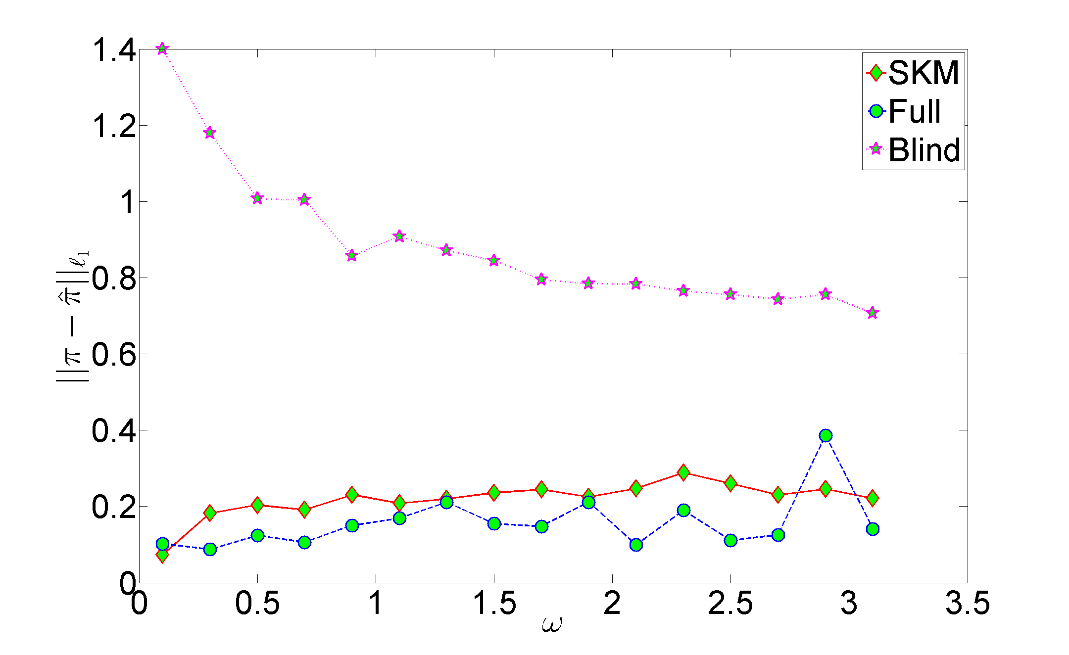
We present a comparison of the performance, measured by the $\ell_{1}$ distance between the true $\pi$ and the estimate $\hat{\pi}$, of the sparse KME compared to the full KME. We have done this for different values of $\pi$, meaning different locations of $\pi$ inside the simplex. To do so, we sampled $\pi$ from the simplex using the Dirichlet distribution with different concentration parameter $\omega$. As a reminder to the reader, a small value of $\omega$ implies sparse values of $\pi$ are most probable, $\omega=1$ means any value of $\pi$ is equally probable, and $\omega>1$ means values of $\pi$ for which all its entries are of similar value are most probable. We varied $\omega$ over the set $\left\{.1,.2,\dots,3.1\right\}$.

References

- [1] E. Cruz Cortés and C. Scott, “Scalable sparse approximation of a sample mean,” in Proc. 2014 IEEE Int. Conf. on Acoustic, Speech and Signal Processing (ICASSP), 2014, pp. 5274–5278.
- [2] E. Cruz Cortés and C. Scott, “SKM Matlab code,” http://web.eecs.umich.edu/~cscott/code.html#skm, 2015, last accessed February-2015.
- [3] D. M. Titterington, G. D. Murray, L. S. Murray, D. J. Spiegelhalter, A. M. Skene, J. D. F. Habbema, and G. J. Gelpke, “Comparison of discrimination techniques applied to a complex data set of head injured patients,” Journal of the Royal Statistical Society. Series A (General), pp. 145–175, 1981.
- [4] D. J. Hand, “A comparison of two methods of discriminant analysis applied to binary data,” Biometrics, pp. 683–694, 1983.
- [5] M. J. Desforges, P. J. Jacob, and J. E. Cooper, “Applications of probability density estimation to the detection of abnormal conditions in engineering,” Proceedings of the Institution of Mechanical Engineers, Part C: Journal of Mechanical Engineering Science, vol. 212, no. 8, pp. 687–703, 1998.
- [6] D. Yeung and C. Chow, “Parzen-window network intrusion detectors,” in Pattern Recognition, 2002. Proceedings. 16th International Conference on, vol. 4. IEEE, 2002, pp. 385–388.
- [7] M. Markou and S. Singh, “Novelty detection: a review—part 1: statistical approaches,” Signal processing, vol. 83, no. 12, pp. 2481–2497, 2003.
- [8] V. Chandola, A. Banerjee, and V. Kumar, “Anomaly detection: a survey,” ACM Computing Surveys (CSUR), vol. 41, no. 3, p. 15, 2009.
- [9] Y. Cheng, “Mean shift, mode seeking, and clustering,” Pattern Analysis and Machine Intelligence, IEEE Transactions on, vol. 17, no. 8, pp. 790–799, 1995.
- [10] I. Steinwart and A. Christmann, Support Vector Machines. Springer, 2008.
- [11] A. Smola, A. Gretton, L. Song, and B. Schölkopf, “A Hilbert space embedding for distributions,” in Algorithmic Learning Theory. Springer, 2007, pp. 13–31.
- [12] A. Gretton, K. M. Borgwardt, M. J. Rasch, B. Schölkopf, and A. Smola, “A kernel two-sample test,” The Journal of Machine Learning Research, vol. 13, no. 1, pp. 723–773, 2012.
- [13] K. Fukumizu, L. Song, and A. Gretton, “Kernel Bayes’ rule,” in Advances in neural information processing systems, 2011, pp. 1737–1745.
- [14] P. Gurram and H. Kwon, “Contextual SVM for hyperspectral classification using Hilbert space embedding,” in Geoscience and Remote Sensing Symposium (IGARSS), 2012 IEEE International. IEEE, 2012, pp. 5470–5473.
- [15] C. Scovel, D. Hush, I. Steinwart, and J. Theiler, “Radial kernels and their reproducing kernel hilbert spaces,” Journal of Complexity, vol. 26, no. 6, pp. 641–660, 2010.
- [16] J. A. Tropp, “Greed is good: Algorithmic results for sparse approximation,” Information Theory, IEEE Transactions on, vol. 50, no. 10, pp. 2231–2242, 2004.
- [17] S. G. Mallat and Z. Zhang, “Matching pursuits with time-frequency dictionaries,” Signal Processing, IEEE Transactions on, vol. 41, no. 12, pp. 3397–3415, 1993.
- [18] B. Jeon and D. A. Landgrebe, “Fast parzen density estimation using clustering-based branch and bound,” Pattern Analysis and Machine Intelligence, IEEE Transactions on, vol. 16, no. 9, pp. 950–954, 1994.
- [19] M. Girolami and C. He, “Probability density estimation from optimally condensed data samples,” Pattern Analysis and Machine Intelligence, IEEE Transactions on, vol. 25, no. 10, pp. 1253–1264, 2003.
- [20] S. Chen, X. Hong, and C. J. Harris, “An orthogonal forward regression technique for sparse kernel density estimation,” Neurocomputing, vol. 71, no. 4, pp. 931–943, 2008.
- [21] M. Schafföner, E. Andelic, M. Katz, S. E. Krüger, and A. Wendemuth, “Memory-effcient orthogonal least squares kernel density estimation using enhanced empirical cumulative distribution functions,” in International Conference on Artificial Intelligence and Statistics, 2007, pp. 428–435.
- [22] D. W. Scott and W. F. Szewczyk, “From kernels to mixtures,” Technometrics, vol. 43, no. 3, pp. 323–335, 2001.
- [23] A. R. Runnalls, “Kullback-Leibler approach to Gaussian mixture reduction,” Aerospace and Electronic Systems, IEEE Transactions on, vol. 43, no. 3, pp. 989–999, 2007.
- [24] D. Schieferdecker and M. F. Huber, “Gaussian mixture reduction via clustering,” in Information Fusion, 2009. FUSION’09. 12th International Conference on. IEEE, 2009, pp. 1536–1543.
- [25] M. A. T. Figueiredo and A. K. Jain, “Unsupervised learning of finite mixture models,” Pattern Analysis and Machine Intelligence, IEEE Transactions on, vol. 24, no. 3, pp. 381–396, 2002.
- [26] P. Bruneau, M. Gelgon, and F. Picarougne, “Parsimonious reduction of Gaussian mixture models with a variational-Bayes approach,” Pattern Recognition, vol. 43, no. 3, pp. 850–858, 2010.
- [27] L. Greengard and V. Rokhlin, “A fast algorithm for particle simulations,” Journal of computational physics, vol. 73, no. 2, pp. 325–348, 1987.
- [28] A. G. Gray and A. W. Moore, “N-body problems in statistical learning,” in NIPS, vol. 4, 2000, pp. 521–527.
- [29] C. Yang, R. Duraiswami, N. A. Gumerov, and L. Davis, “Improved fast Gauss transform and efficient kernel density estimation,” in Computer Vision, 2003. Proceedings. Ninth IEEE International Conference on. IEEE, 2003, pp. 664–671.
- [30] D. Lee, A. Gray, and A. W. Moore, “Dual-tree fast Gauss transforms,” in Advances in Neural Information Processing Systems 18 (Dec 2005), Y. Weiss, B. Scholkopf, and J. Platt, Eds. MIT Press, 2006.
- [31] Y. Zheng, J. Jestes, J. M. Phillips, and F. Li, “Quality and efficiency for kernel density estimates in large data,” in Proceedings of the 2013 international conference on Management of data. ACM, 2013, pp. 433–444.
- [32] J. M. Phillips, “-samples for kernels,” in Proceedings of the Twenty-Fourth Annual ACM-SIAM Symposium on Discrete Algorithms. SIAM, 2013, pp. 1622–1632.
- [33] S. Joshi, R. V. Kommaraji, J. M. Phillips, and S. Venkatasubramanian, “Comparing distributions and shapes using the kernel distance,” in Proceedings of the twenty-seventh annual symposium on Computational geometry. ACM, 2011, pp. 47–56.
- [34] J. Zhao and D. Meng, “FastMMD: Ensemble of circular discrepancy for efficient two-sample test,” NIPS Workshop on Randomized Methods for Machine Learning, 2013.
- [35] P. Drineas and M. W. Mahoney, “On the Nyström method for approximating a gram matrix for improved kernel-based learning,” The Journal of Machine Learning Research, vol. 6, pp. 2153–2175, 2005.
- [36] S. Kumar, M. Mohri, and A. Talwalkar, “Sampling methods for the Nyström method,” The Journal of Machine Learning Research, vol. 13, no. 1, pp. 981–1006, 2012.
- [37] W. B. March and G. Biros, “Far-field compression for fast kernel summation methods in high dimensions,” arXiv preprint arXiv:1409.2802, 2014.
- [38] Z. Noumir, P. Honeine, and C. R., “One-class machines based on the coherence criterion,” in Statistical Signal Processing Workshop (SSP), 2012 IEEE. IEEE, 2012, pp. 600–603.
- [39] V. V. Vazirani, Approximation algorithms. Springer, 2001.
- [40] T. F. Gonzalez, “Clustering to minimize the maximum intercluster distance,” Theoretical Computer Science, vol. 38, pp. 293–306, 1985.
- [41] D. S. Hochbaum, Approximation algorithms for NP-hard problems. PWS Publishing Co., 1996.
- [42] J. Duchi, S. Shalev-Shwartz, Y. Singer, and T. Chandra, “Efficient projections onto the -ball for learning in high dimensions,” in Proceedings of the 25th international conference on Machine learning. ACM, 2008, pp. 272–279.
- [43] J. B. Tenenbaum, V. de Silva, and J. C. Langford, “A global geometric framework for nonlinear dimensionality reduction,” Science, vol. 290, pp. 2319–2323, 2000.
- [44] W. G. Finn, K. M. Carter, R. Raich, L. M. Stoolman, and A. O. Hero, “Analysis of clinical flow cytometric immunophenotyping data by clustering on statistical manifolds: Treating flow cytometry data as high-dimensional objects,” Cytometry Part B: Clinical Cytometry, vol. 76, no. 1, pp. 1–7, 2009.
- [45] D. M. Titterington, “Minimum distance non-parametric estimation of mixture proportions,” Journal of the Royal Statistical Society, vol. 45, no. 1, pp. 37–46, 1983.
- [46] Y. LeCun, “The mnist database,” http://yann.lecun.com/exdb/mnist, 2014, last accessed 24-September-2014.
- [47] Y. LeCun, L. Bottou, Y. Bengio, and P. Haffner, “Gradient-based learning applied to document recognition,” Proceedings of the IEEE, vol. 86, no. 11, pp. 2278–2324, 1998.
- [48] D. Comaniciu and P. Meer, “Mean shift: A robust approach toward feature space analysis,” Pattern Analysis and Machine Intelligence, IEEE Transactions on, vol. 24, no. 5, pp. 603–619, 2002.
- [49] B. Finkston, “Mean shift clustering,” http://www.mathworks.com/matlabcentral/fileexchange/10161-mean-shift-clustering, 2014, last accessed 24-September-2014.
- [50] Y. Chen, C. R. Genovese, and L. Wasserman, “Enhanced mode clustering,” arXiv preprint arXiv:1406.1780, 2014.
- [51] A. Gionis, P. Indyk, and R. Motwani, “Similarity search in high dimensions via hashing,” in VLDB, vol. 99, 1999, pp. 518–529.
- [52] A. Andoni and P. Indyk, “Near-optimal hashing algorithms for approximate nearest neighbor in high dimensions,” in Foundations of Computer Science, 2006. FOCS’06. 47th Annual IEEE Symposium on. IEEE, 2006, pp. 459–468.
- [53] G. Shakhnarovich, “Locality Sensitive Hashing,” http://ttic.uchicago.edu/~gregory, 2014, last accessed 24-September-2014.
- [54] A. Andoni, “LSH algorithm and implementation,” http://www.mit.edu/~andoni/LSH, 2014, last accessed 24-September-2014.
- [55] J. E. Chacón, “A population background for nonparametric density-based clustering,” arXiv preprint arXiv:1408.1381, 2014.
- [56] T. Jaakkola, M. Diekhans, and D. Haussler, “Using the fisher kernel method to detect remote protein homologies.” in ISMB, vol. 99, 1999, pp. 149–158.
- [57] F. Wilcoxon, “Individual comparisons by ranking methods,” Biometrics bulletin, vol. 1, no. 6, pp. 80–83, 1945.