Biased Online Parameter Inference for State-Space Models
BY YAN ZHOU & AJAY JASRA
Department of Statistics & Applied Probability,
National University of Singapore, Singapore, 117546, SG.
E-Mail: stazhou@nus.edu.sg, staja@nus.edu.sg
Abstract
We consider Bayesian online static parameter estimation for state-space models. This is a very important problem, but is very computationally challenging
as the state-of-the art methods that are exact, often have a computational cost that grows with the time parameter; perhaps the most successful algorithm
is that of SM [9]. We present a version of the SM algorithm which has computational cost that does not grow with the time parameter.
In addition, under assumptions, the algorithm is shown to provide consistent estimates of expectations w.r.t. the posterior. However, the cost to achieve this consistency can be exponential
in the dimension of the parameter space; if this exponential cost is avoided, typically the algorithm is biased.
The bias is investigated from a theoretical perspective and, under assumptions, we find that the bias does not accumulate as the time parameter grows.
The algorithm is implemented on several Bayesian statistical models.
Keywords: State-Space Models; Bayesian Inference; Sequential Monte Carlo.
1 Introduction
We consider a state-space models, that is, a pair of discrete-time stochastic processes, and . The hidden process is a Markov chain and the joint density for observations of the hidden process and the observations is
where , , and , , is a static parameter with prior . In particular, it is of interest to infer the posterior on , conditional upon () as the time parameter grows. This problem is of interest in a wide variety of applications, including econometrics, finance and engineering; see for instance [5].
In general, even if is fixed, the posterior cannot be computed exactly and one often has to resort to numerical methods, for example by using sequential Monte Carlo (SMC) (see e.g. [16]). SMC makes use of a collection of proposal densities and sequentially simulates from these samples, termed particles. In most scenarios it is not possible to use the distribution of interest as a proposal. Therefore, one must correct for the discrepancy between proposal and target via importance weights. In the majority of cases of practical interest, the variance of these importance weights increases with algorithmic time. This can, to some extent, be dealt with via a resampling procedure consisting of sampling with replacement from the current weighted samples and resetting them to . However, as is well known in the literature, due to the path degeneracy problem for particle filters, when is a random variable SMC methods do not always work well; see the review of [20] for details. This has lead to a wide variety of techniques being developed, including [9, 11, 17, 18, 21]; see [20] for a full review.
The method which one might consider to be the state-of-the-art for the Bayesian online static parameter estimation for state-space models, is that in [9]. This approach combines the methods of SMC samplers [14] and particle Markov chain Monte Carlo (PMCMC) [1]. The method provides consistent estimates (that is, as the number of samples grows) of expectations w.r.t. the posterior on , as the time parameter grows. The method has been shown to work well in practice, but has one major issue; the computational cost of the application of PMCMC kernels grows as the time parameter grows; whilst the amount of times that the application of the kernel may stablize, one will still need to apply the kernel during the algorithm (although a variety of tricks can be used to reduce the cost; see [19]). We present a version of the SM algorithm which has computational cost that does not grow with the time parameter. In addition, under assumptions, the algorithm is shown to provide consistent estimates of expectations w.r.t. the posterior. However, the cost to achieve this consistency can be exponential in the dimension of the parameter space; if this exponential cost is avoided, typically the algorithm is biased. The bias is investigated from a theoretical perspective and, under assumptions, we find that the bias does not accumulate as the time parameter grows.
Our approach is based upon breaking up the observations into blocks of observations; an approach used, differently, in other articles such as [8, 11, 18]. The idea is simply to develop a ‘perfect’ SM algorithm which has computational cost that does not grow with the time parameter; in practice, one cannot implement this algorithm and so one must approximate it. Our approach simply uses the approximation of an appropriate target from the previous block. It is remarked that if the posterior exhibits concentration/Bernstein-Von Mises properties as the time parameter grows, then alternative schemes are relevant, which could be prefered to the ideas here; however, such properties do not always hold. See for instance the work of [15] in the context of MLE for relatively weak conditions; the properties of the MLE can impact on the concentration/Bernstein-Von Mises properties of the posterior (see e.g. [4]).
2 Algorithm
2.1 Notations
Let be a measurable space. The notation denotes the class of bounded and measurable real-valued functions. dentes the continuous, bounded measurable real-valued functions on . The supremum norm is written as . is the set of probability measures on . We will consider non-negative operators such that for each the mapping is a finite non-negative measure on and for each the function is measurable; the kernel is Markovian if is a probability measure for every . For a finite measure on , real-valued and measurable
We also write . denotes the total variation distance.
2.2 SM
SMC2 uses SMC to sample the following sequence of targets, for a fixed
with , where
with for any . Throughout, we write the normalizing constant of as . We make the following defintion for notational convenience in the sequel:
| (1) | |||||
| (2) |
We provide a Feynman-Kac representation of the SMC2 algorithm which facilitates theoretical analysis and will assist our subsequent notations. Let and set
and for any
where is invariant (i.e. typically a particle marginal Metropolis-Hastings (PMMH) kernel [1]). Then we set
and
The SMC algorithm which approximates the time marginal
will have joint law:
| (3) |
where is the usual selection-mutation operator and is the empirical measure of the particles. It is easily shown that by approximating one can approximate the posterior on and given ; see [9, 13]. We note that, typically one will apply the kernel when dynamic resampling is performed; however the form of the algorithm is simple to describe with resampling at each time step.
2.3 Perfect Algorithm
One issue with the above algorithm is that whenever the kernel is applied, one must sample trajectories of the hidden states which grow with the time parameter. Thus, even if resampling is dynamically performed, leading to an application of , the cost of the algorithm will increase with the time parameter. So one can say whilst SM is a very powerful algorithm, it is not an online algorithm. Here we present an ‘ideal’ or perfect version of the algorithm that has computational cost which does not grow with time, but cannot be implemented in general. This algorithm will provide the basis for our biased algorithm in the next section.
To begin, we set which in principle can grow and which is fixed. The parameter will represent the maximum length of the trajectory of the hidden state, which one wants to sample. We define the following target probabilities:
| (4) | |||||
and
| (5) |
where is as (1) and
If one can approximate the targets above one can approximate the posterior on and given . As we will see below, our algorithm to achieve this cannot be implemented in practice, but has the benefit that the computational cost per-time step cannot grow beyond a given bound.
2.3.1 Algorithm
For one can run the SM algorithm as in Section 2.2. That is to run the algorithm with law (3) until time . We will add a final time step that will resample the particles according to . That is, defining as the Dirac measure, we sample from
For the subsequent blocks, we make the following definitions. Let , , , , and . Now let
Set
Define as a Markov kernel of invariant density , such as a PMMH kernel. Then define
where and is as (2). Set as a Dirac mass. Finally, for , and probability density on define
Then the perfect algorithm has joint law for ,
where is the empirical measure of the particles at time .
2.3.2 Remarks
Set, for ,
and , then we note that for , integrable
so that one can estimate expectations w.r.t. via
| (6) |
2.4 Approximate Algorithm
The problem with the previous algorithm is that one can seldom evaluate nor sample from it perfectly. We introduce the following algorithm, which will sample from the following targets. For the first block, one can run the SM algorithm to target the sequence (4). At the subsequent blocks, one is unable to evaluate the target, nor sample from the proposals. We propose the following approximate targets to replace (5):
| (7) |
with , samples from the algorithm at the previous block, which we shall describe how to obtain and a kernel density whose bandwidth may depend on . At the end of a block of the algorithm, we just take , as the samples we have obtained, taking the first of the tuples of (as the samples are exchangeable). Using standard SMC theory, which we will expand upon, one can prove that if the bandwidth of appropriately depends on that at least will converge almost surely (in an appropriate sense) to as grows, hence providing the justification of the approximation introduced.
Set
Then the approximate algorithm has joint law for ,
where is the empirical measure of the particles at time . An estimate of the form (6) can be used to estimate the targets. Note that the cost of the algorithm is not as one does not need to evaluate , even in the PMMH steps.
2.5 Related Simulation Methods and Alternatives
Similar, but different, ideas have appeared in several articles including [2, 6, 11]. These ideas are considered in the context of hidden Markov models and partially observed point processes respectively. The key differences of our work to [6, 11] ([2] is for maximum likelihood estimation (MLE)) are as follows. In the context of [6] we do not use a type of ‘sequential MCMC’, in that our approach can be used explicitly for online Bayesian parameter estimation. The approach of [11] is less general, where the particles are not updated with PMCMC, and one has a block length of 1.
Alternatives to the approach outlined above are; (i) a form of sequential PMCMC in the spirit of [6] or (ii) to use an over-lapping or sliding window. For (i), one expects that the cost is higher than the above algorithm, and online (filtered) estimates are not available. For (ii) the cost may be higher, but, in simulation studies, we did not find any obvious improvement in practice. We also remark that our approximate algorithm uses kernel density estimation, but, in principle, any approximation scheme could be used; this is demonstrated in Section 4 where the method in [8] is used in place of a kernel density estimate. In practice, the algorithm is implemented with dynamic resampling according to the effective sample size.
3 Theoretical Results
Throughout, it is supposed that for any , .
3.1 Consistency
We will now show that, under a specific choice of the bandwidth and under some mathematical assumptions, the algorithm just presented is consistent. We set ; it is supposed that for any fixed , . For simplicity we denote (resp. ), as (resp. ).
- (A1)
We have
- –
,
- –
- –
.
- –
- (A2)
For each , , , there exists a such that for every
- (A3)
We have , in addition there exist a such that for every .
- (A4)
For any , , the function is continuous at uniformly in ; also .
The first three assumptions are from [10] to allow convergence of the SMC estimate of the kernel density and the final assumption is from [3]. We set
Let denote convergence in probability as . We now have the following result whose proof is in Appendix A.
Theorem 3.1.
Assume (A1-4). Then for each , , and we have
and in particular for every
Remark 3.1.
The result here is essentially qualitative. In order to obtain consistency, one must adopt an exponential effort in and so one would only run (with the choice of as in (A(A3))) over the exact algorithm if the time horizon is long and is small. In practice one will decouple and , leading to estimates which are biased, even if . We will now study the bias.
3.2 Bias
We now investigate the asymptotic (in ) bias of the approach. We make the following hypothesis:
- (A5)
There exists a such that for any :
There exists an and for any , there exists a such that for any probability density on
We write the limiting version of (7) as (which one can easily prove exists, for any ). For a bounded we define the bias as
We have the following result whose proof is in Appendix B.
Theorem 3.2.
Assume (A(A5)). Then there exist a , such that for any :
Remark 3.2.
The result indicates that some of the bias can fall at a geometric rate as grows. Note, that the bias cannot disappear once, one block is wrong (which is by assumption in the statement of the theorem). The result also provides the reassuring point that bias’ do not accumulate as the number of blocks grow, albeit under strong assumptions.
4 Simulations
4.1 Gaussian linear model
4.1.1 Model and algorithm setting
We consider the following Gaussian model,
where is the density function of a Normal distribution with mean and variance .
The data is simulated from , with 10,000 time steps. The algorithms are implemented with fixed to and the other two being estimated. That is, the parameter is .
We consider three algorithms. First, due to the simple structure of the model, we can obtain exact evaluation of through a Kalman filter. We will replace the particle filter in the SM algorithm with the Kalman filter; this results in a regular SMC algorithm. This is used to provide accurate unbiased estimators when comparing algorithms. The second is the SM algorithm and the third is the proposed new algorithm, which is termed SMFW. The PMCMC step in each algorithm is constructed as a two-block Metropolis random walk, with a Normal kernel on the logarithm scale.
With the Kalman filter, the computational cost of is negligible and thus we use a large number of -particles, . This allows us to obtain unbiased posterior estimators with very small variance. As a result, this provides a good baseline for the comparison of the other two algorithms.
For the SM algorithm, we use particles for the SMC algorithm and particles. For simplicity, the value of is fixed through the time line.
For the SMFW algorithm, we set and . As we will see later, despite the increased number of the -particles, the computational cost is still significantly lower than SM, in addition to be upper bounded per time step. The kernel density estimate (KDE) is bivariate Normal on the logarithm scale, with covariance matrix taken a diagonal form, where is the identity matrix of rank two. We consider , and . Three widths of each fixed window , and are also considered.
4.1.2 Results
In Figure 1 to 3 we show the average of estimates over 30 simulations, given different bandwidth and window width . The first 125 time steps are cutoff from the graphs, during which time the SMFW algorithm is exactly the same as the SM algorithm.


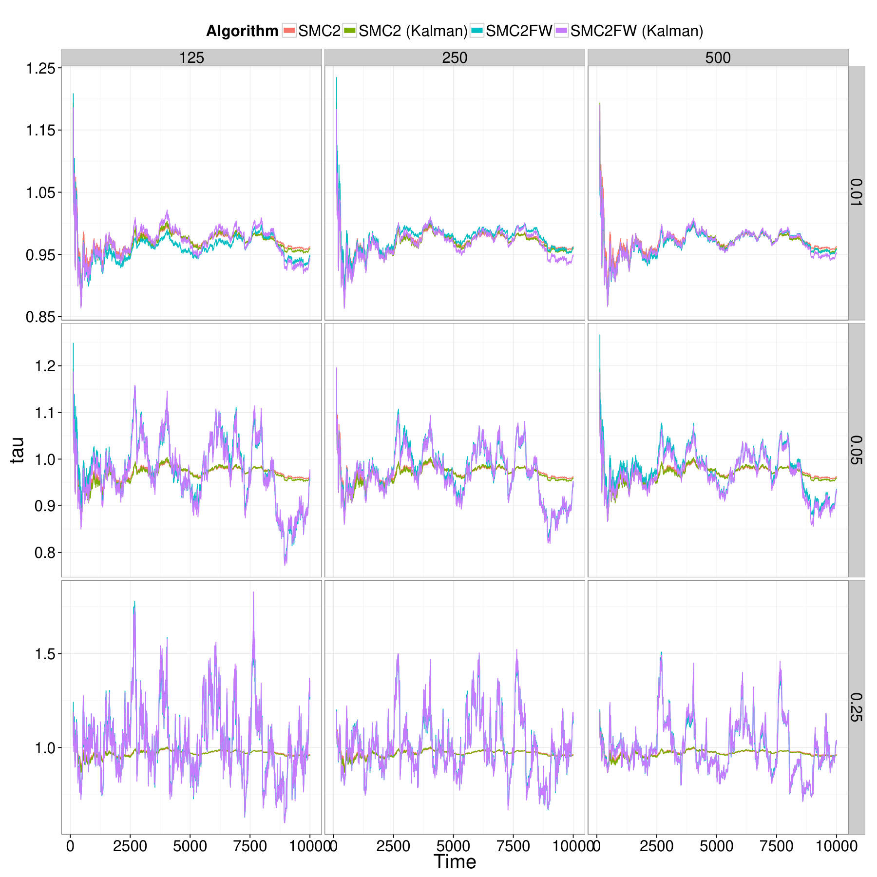
Algorithms labeled with “Kalman” means a Kalman filter is used in place of a particle filter and thus exact values of are calculated instead of approximations. In this case, the results show the behavior of the SMFW algorithm when . However, in this particular example, errors introduced by the particle filter approximation is minimal as shown in the graphs.
It is as expected that the longer the window width, the better the SMFW algorithms perform. The choice of the bandwidth has a more dramatic effect on the performance. With the algorithms give almost exact results even for . On the other hand, with , the errors are numerous. For the state , neither the bandwidth nor the window width affect the results in any observable way. For the parameters, and provides the best results.
In Figure 4 the MSE of the two algorithms are shown, using the results obtained with a SMC algorithm using Kalman filters (SM (Kalman) in previous figures) as an unbiased, accurate estimate of the true posterior means. It can be seen that for the state , the results are mixed. For the parameter the SM algorithm has a smaller MSE while the opposite is true for the parameter. It shall be noted that, the SMFW algorithm use while the SM algorithm only use . However, despite the large difference of the numbers of -particles, the SMFW algorithm is still significantly more computationally cost efficient. It took about thirty minutes for a single run of the SMFW algorithm under this setting while it took about five hours for the SM algorithm. More importantly, the cost of SMFW is bounded per time step, and thus it is possible to obtain better results than SM for all parameters while having a bounded, smaller cost in the long run.
4.2 Lévy-driven stochastic model
4.2.1 Model and algorithm setting
We consider the Lévy-driven stochastic volatility model, applied to 1,000 recent S&P 500 data from September 17, 2010 to September 8, 2014. The data are obtained as logarithm return of the daily adjusted close price, and then normalized to unity variance. The data is plotted in Figure 5. There are considerably much larger volatility at the beginning of the series. It becomes much more stable in the middle and slightly larger at the end.
The model we employed to analyze this data is the same as in [1] and we use the same notations and formulation as in that paper. The model has four parameters and a two-dimensional state where is the time interval and in this example it set to constant .
We consider three algorithms. First, the SM algorithm with and . Second, the SMFW algorithm with the same number of particles. The same Normal KDE approximation is used as in the last example. Various bandwidths of the kernel were considered, and is chosen. The last, the idea coupled with the parallel particle filter algorithm (PPF) [8], instead of the KDE approximation, is considered. The latter two algorithms use a window width . We found that further increasing the window width does not improve results in a significant manner.
The algorithms again use Normal kernels on logarithm scales for the PMMH proposals. Using results from the particle filter paper, we believe that and are strongly correlated and they are updated in one block of PMCMC move while and are updated individually in their own block. The proposal scales are calibrated on-line using the moments estimates from the sampler.
4.2.2 Results
In Figure 6 we show the average of estimates over 20 simulations. All three algorithms give similar results. Compared to results from the SM algorithm, the SMFW algorithm give slightly better result than that of the SMFW-PPF one.
One feature that was mentioned in Section 3, but not shown clearly in the early simple Gaussian linear example, is that the bias of the online algorithms does not accumulate over time. For instance, consider the state, though non-trivial errors can be observed for both on-line algorithms in the early time steps, they were not carried on to later times.
In addition to the estimates, prediction of the variance (square of volatility), is also calculated as . Since the transition density is not of a closed form, its expectation is estimated with 100 samples of generated for each value of in the particle system. The outer expectation is approximated with the particle system at time . The results for the three algorithms are plotted in Figure 7 against the squared log-returns.
4.2.3 Summary
Through two examples, it is shown that with some careful choice of the KDE bandwidth, or using the parallel particle filter algorithm, which does not require this layer of tuning and an appropriate window width, it is possible to obtain results competitive to the SM algorithm with only a fraction of computational cost. In the Lévy-driven stochastic model example, the theoretical feature that the bias does not accumulate over time is demonstrated.
5 Summary
In this article we have presented a method for Bayesian online static parameter estimation for state-space models. Our method is such that the computational cost does not grow with the time parameter and moreover, the algorithm can be shown to be consistent, although, the cost is then exponential in the dimension of the static parameter. We have additionally shown that the asymptotic bias, under strong assumptions, does not grow with time.
There are several avenues for future work. First is the use of alternative approximation schemes in our algorithm; we have relied on kernel density estimation, but there are other schemes which could be used. Second, in our work, we have investigated the asymptotic bias. However, as is clear in the proofs, then the consecutive blocks are independent and one thus expects that the study of the finite sample bias is significantly more challenging; an investigation of this is warranted.
Acknowledgements
This research was supported by a Singapore Ministry of Education Academic Research Fund Tier 1 grant (R-155-000-156-112). We thank Alex Beskos & Alex Thiery for many useful conversations on this work.
Appendix A Technical Results: Consistency
Proof of Theorem 3.1.
For the result follows by standard theory; see [10, 12, 13]. We first consider . Denote by the algebra generated by the particle system up-to time and expectations w.r.t. the law of the simulated algorithm as . Then we have
For the first term on the R.H.S. one has by the (conditional) Marcinkiewicz-Zygmund inequality (conditional on the samples are generated independently):
where depends on in (A(A3)); thus converges to zero in probability.
Now, for
, and the denominator converges in probability and by the arguments in [10][Theorem 4.1] the numerator will converge in probability to the appropriate quantity; that is .
For , this converges in probability to by centering by the conditional expectation (given ) and applying the (conditional) Marcinkiewicz-Zygmund inequality for . The term will converge to using the conditional i.i.d. property and the fact that converges in probability to .
For , we consider:
The first term is dealt with via the (conditional) Marcinkiewicz-Zygmund inequality as above. For as converges in probability to , we need only consider
The last term on the R.H.S. converges to zero by the above calculations. So we focus on the first term on the R.H.S. we have
Let be given. By (A(A4)) there exists independent of such that for any probability density with we have that . Consider the event:
Then
By the convergence in probability of here is an such that for each we have . Hence, for any :
and as was arbitrary, the term of interest goes to zero in ; this completes the proof. The proof can also be repeated if one considers a as part of the function (the argument is almost the same). The proofs at subsequent times follow the above arguments and are omitted for brevity. ∎
Appendix B Proofs for Bias
In the context of the proof for the bias, we need only consider one block (as will become apparent in the proof), as blocks are independent in the asymptotic bias. In addition, one significantly simplify the notations by simply considering two Feynman-Kac formula of steps, with different initial distributions, the same potentials and different Markov kernels on measurable spaces . Thus, for the two Feynman-Kac time marginals:
with
This corresponds to our case, as the potentials are the same, with the Markov kernels and initial distributions different. Our proofs will depend a lot on the Bayes rule, which we now recall, for
We use the notation , (with the convention when , one returns ). Our assumption (A(A5)) under the modified notation is
- •
There exist a such that for every
- •
There exist a and for , such that for each every
Recall that the final Markov kernel is a Dirac measure.
Proof of Theorem 3.2.
Remark B.1.
As one can see from inspection of the proof, the difference in initial distribution does not impact the bound. Moreover, the difference in Markov kernels is controlled, leading to a control of the bias; such a latter property is not obvious a priori and needs to be proved. As is evident from the proof, it does not matter which block one considers, under our assumptions.
Proof.
Proof.
We have
Now, by (A(A5)), for any one can write
where is a Markov kernel:
Thus
from which one easily concludes. ∎
The following Lemma just collects some results of [12] into a convenient form for use in the above proofs. We make the following defintions for , : ,
and . For a bounded and measurable real-valued function we denote
References
- [1] Andrieu, C., Doucet, A. & Holenstein, R. (2010). Particle Markov chain Monte Carlo methods (with discussion). J. R. Statist. Soc. Ser. B, 72, 269–342.
- [2] Andrieu, C., Doucet, A., & Tadić, V. (2009). On-line parameter estimation in general state-space models using pseudo-likelihood. Unpublished Technical Report.
- [3] Beskos, A., Jasra, A., Kantas, N. & Thiery, A. (2014). On the convergence of adaptive sequential Monte Carlo methods. arXiv preprint.
- [4] Borwanker, J., Kallianpur, G., & Prakasa Rao, B.L.S. (1971). The Bernstein-Von Mises theorem for Markov processes. Ann. Math. Stat., 42, 1241–1253.
- [5] Cappé, O., Ryden, T, & Moulines, É. (2005). Inference in Hidden Markov Models. Springer: New York.
- [6] Centanni, S., Minozzo, M. (2006). A Monte Carlo approach to filtering for a class of marked doubly stochastic Poisson processes. Journal of the American Statistical Association, 101, 1582–1597.
- [7] Cérou, F., Del Moral, P. & Guyader, A. (2011). A non-asymptotic variance theorem for un-normalized Feynman-Kac particle models. Ann. Inst. Henri Poincare, 47, 629–649.
- [8] Chan, H. P., Heng, C. W. & Jasra, A. (2014). Theory of parallel particle filters for hidden Markov models. arXiv preprint.
- [9] Chopin, N., Jacob, P. & Papaspiliopoulos, O. (2013). SM: A sequential Monte Carlo algorithm with particle Markov chain Monte Carlo updates. J. R. Statist. Soc. B, 75, 397–426.
- [10] Crisan, D. & Miguez, J. (2014). Particle-kernel estimation of the filter density in state-space models. Bernoulli, 20, 1879–1929.
- [11] Crisan, D. & Miguez, J. (2014). Nested particle filters for online parameter estimation in discrete-time state-space Markov models. arXiv preprint.
- [12] Del Moral, P. (2004). Feynman-Kac Formulae: Genealogical and Interacting Particle Systems with Applications. Springer: New York.
- [13] Del Moral, P. (2013). Mean Field Simulation for Monte Carlo Integration. Chapman & Hall: London.
- [14] Del Moral, P., Doucet, A. & Jasra, A. (2006). Sequential Monte Carlo samplers. J. R. Statist. Soc. B, 68, 411–436.
- [15] Douc, R., Moulines, E., Olsson, J. & Van Handel, R. (2011). Consistency of the maximum likelihood estimator for general hidden Markov models. Ann. Statist., 39, 474-513.
- [16] Doucet, A. & Johansen, A. (2011). A tutorial on particle filtering and smoothing: Fifteen years later. In Handbook of Nonlinear Filtering (eds. D. Crisan et B. Rozovsky), Oxford University Press: Oxford.
- [17] Fearnhead, P. (2002). MCMC, sufficient statistics and particle filters. J. Comp. Graph. Statist., 11, 848–862.
- [18] Gilks, W. R. & Berzuini, C. (2001). Following a moving target - Monte Carlo inference for dynamic Bayesian models. J. R. Statist. Soc. B, 63, 127–146.
- [19] Jacob, P., Murray, L. & Rubenthaler, S. (2015). Path storage in the particle filter. Statist. Comp. (to appear).
- [20] Kantas, N., Doucet, A., Singh, S.S., Maciejowski, J. M., & Chopin, N. (2015). On Particle Methods for Parameter Estimation in State-Space Models. Statist. Sci. (to appear).
- [21] Polson, N.G., Stroud, J.R. & Müller P. (2008). Practical filtering with sequential parameter learning. J. R. Statist. Soc. B, 70, 413–428.