Loop braiding statistics in exactly soluble 3D lattice models
Abstract
We construct two exactly soluble lattice spin models that demonstrate the importance of three-loop braiding statistics for the classification of 3D gapped quantum phases. The two models are superficially similar: both are gapped and both support particle-like and loop-like excitations similar to that of charges and vortex lines in a gauge theory. Furthermore, in both models the particle excitations are bosons, and in both models the particle and loop excitations have the same mutual braiding statistics. The difference between the two models is only apparent when one considers the recently proposed three-loop braiding process in which one loop is braided around another while both are linked to a third loop. We find that the statistical phase associated with this process is different in the two models, thus proving that they belong to two distinct phases. An important feature of this work is that we derive our results using a concrete approach: we construct string and membrane operators that create and move the particle and loop excitations and then we extract the braiding statistics from the commutation algebra of these operators.
I Introduction
The discovery of quantum Hall states and more recently, topological insulators[1, 2], has taught us that there are many different types of gapped quantum many body systems. In order to understand the relationship between these systems, it is useful to divide them into classes in such a way that the members of each class share the same qualitative properties. Typically these classes are defined as follows: two gapped Hamiltonians and are assigned to the same class if they can be adiabatically connected to one another — that is, if there exists a one parameter family of interpolating Hamiltonians with (1) , and (2) a finite energy gap for all , . The different classes of Hamiltonians are then called “gapped phases.”
The precise definition of gapped phases depends on what type of systems we wish to consider. For example, if we are interested in systems with particular symmetries, then it is natural to assign and to the same phase if there exists an interpolating Hamiltonian which is both gapped and invariant under the relevant symmetries. Including such symmetry constraints typically leads to a finer classification of gapped phases, as illustrated by the example of topological and conventional insulators.[1, 2]
In this paper, we consider the coarsest possible classification scheme: that is, we do not impose any symmetry constraints and we say that two gapped Hamiltonians and belong to the same phase if they can be adiabatically connected by any interpolating Hamiltonian with local interactions. Our starting point is a basic question: how can we tell whether or not two gapped Hamiltonians belong to the same phase?
This question has an appealing answer in the case of two dimensional (2D) systems. 11 1 The 1D case is less interesting, since it is known that in the absence of symmetry all 1D bosonic systems belong to the same phase[29, 31, 32, 33, 30, 42] while all 1D fermionic systems belong to one of two phases.[30] To determine whether two gapped 2D Hamiltonians belong to the same phase, one can simply compare the braiding statistics 22 2 Here, when we say braiding statistics, we mean the complete set of algebraic data for anyon systems, including quantum dimensions and fusion rules. For more details, see e.g. Appendix E of Ref. 43. of their quasiparticle excitations. If the braiding statistics data do not match, then the two Hamiltonians must belong to different phases since braiding statistics cannot change under an adiabatic deformation. Conversely, if the braiding statistics do match, then we can almost conclude that the two Hamiltonians belong to the same phase. To reach this conclusion, we simply need to compare one other quantity, namely the thermal Hall conductance[5]. Indeed, according to a plausible (but unproven) conjecture, if two Hamiltonians have the same braiding statistics and the same thermal Hall conductance, then they must be adiabatically connected to one another in the absence of any symmetry constraints.
In the 3D case, our understanding is much more limited. One way to attack the classification problem is to try to generalize the concept of quasiparticle braiding statistics to the 3D case. The simplest generalization begins with the observation that many 3D Hamiltonians support loop-like excitations in addition to particles. Given this observation, we can consider several different types of braiding statistics. First, we can look at the exchange statistics of particle-like excitations. These exchange statistics can take only one of two values for each particle: every particle must be either bosonic or fermionic.33 3 Here, we implicitly exclude 3D layered systems, like a stack of fractional quantum Hall states, from our discussion. Second, we can consider the statistical phase associated with braiding a particle around a loop.[7, 8, 9, 10] Finally, we can look at the statistical phase associated with braiding one loop excitation around another (Fig. 1a).[11, 12, 13] If we combine all of these types of braiding statistics, we can indeed distinguish many different 3D gapped phases.
Interestingly, however, this data is incomplete: Refs. 14, 15 argued that we also need to consider the statistical phase associated with a three-loop braiding process. In this process, one loop is braided around another loop while both are linked to a third loop (Fig. 1b). It is unclear whether the three-loop braiding data is the last piece of the puzzle or whether there exist further distinctions between 3D gapped phases that can only be seen if we consider other braiding processes or other types of probes. However, either way, three-loop braiding statistics has already proven to be useful in certain cases. [16, 17, 18, 19]
One weakness of previous studies of three-loop braiding statistics is that this quantity has only been calculated using indirect and abstract arguments. For example, Ref. 14 computed the three-loop braiding statistics of 3D Dijkgraaf-Witten gauge theories using a dimensional reduction argument which relates the braiding statistics of loops in 3D Dijkgraaf-Witten models to the braiding statistics of particles in 2D Dijkgraaf-Witten models[20]. The approaches of Refs. 15, 16 were also indirect: Refs. 15, 16 computed loop braiding statistics by relating this quantity to modular transformations on a three dimensional torus.
In this paper, we study three-loop braiding statistics using a more concrete approach. We focus on two exactly soluble lattice models and we compute their three-loop braiding statistics by explicitly implementing the loop braiding process on the lattice. Our approach is similar to how quasiparticle braiding statistics is commonly calculated in 2D lattice models[21, 22, 23]: we construct membrane operators that create and move loop-like excitations, and then we extract the three-loop statistics from the commutation algebra of these operators.
The two spin models that we analyze provide an explicit demonstration of the importance of three-loop braiding statistics for distinguishing 3D gapped phases. Indeed, we show that the models share the same particle exchange statistics as well as the same particle-loop and loop-loop braiding statistics. The only difference between the models is that they have different three-loop braiding statistics. Thus, it is only this quantity that reveals that the two models belong to different phases.
The models that we study are not completely new and have appeared previously in the literature in different forms. In particular, the first model is essentially identical to the 3D generalized toric code model[21, 24, 23, 25] corresponding to the group . Thus, the low energy properties of this model are similar to that of conventional gauge theory[26]. The second model can be thought of as a different type of gauge theory. More specifically, this model can be obtained by starting with the spin model in Ref. 27 which describes a nontrivial symmetry-protected topological phase[28, 29, 30, 31, 32, 33, 34] with symmetry, and then coupling this system to a lattice gauge field[26]. We will explain this connection in more detail in a separate publication[35]. In addition to its connection with the spin model in Ref. 27, we believe that the second model belongs to the same phase as one of the exactly soluble Dijkgraaf-Witten models.[20, 36] This conjecture is based on the fact that the braiding statistics in the two systems seem to match one another.
The connection between our models and symmetry-protected topological phases is not accidental: we specifically designed our models to be equivalent to gauged symmetry-protected topological phases, because according to the results of Ref. 14, 15, such gauge theories can support different types of three-loop braiding statistics. The reason that we chose to gauge the spin model from Ref. 27 is that this is one of the simplest known models for a 3D symmetry-protected topological phase with unitary symmetry group.
The rest of the paper is organized as follows. In section II we introduce the two exactly soluble 3D spin models that we will analyze. In section III, we study the particle-like and loop-like excitations of these models by explicitly constructing the string and membrane operators that create and move these excitations. We then compute the braiding statistics of these particles and loops in section IV. Some technical details can be found in the appendices.

II Models
II.1 Hilbert space for the models

The models that we will discuss are spin- systems made up of two species of spins: “blue spins” and “red spins.” The blue spins live on the plaquettes of the cubic lattice and will be denoted by while the red spins live on the plaquettes of the dual cubic lattice and will be denoted by (Fig. 2). In this notation, the eigenstates provide a complete basis for the Hilbert space.
We will often find it convenient to describe spin states using an alternative language based on “membranes.” In the membrane language, each eigenstate corresponds to a spatial configuration of red and blue membranes on the cubic lattice and dual cubic lattice. The dictionary between spin states and membrane configurations is as follows: if we say that the plaquette is occupied by a blue membrane, while if we say that the plaquette is empty. Similarly, if then is occupied by a red membrane while if , then is empty. In this way, each spin state can be equivalently described as a membrane state. We will label our membrane states as where denotes the subset of plaquettes that are occupied by blue membranes, and denotes the subset of plaquettes occupied by red membranes.
II.2 Ground state wave functions
The two models that we will discuss have been engineered to have particular ground states. These ground states are easiest to describe if we assume an infinite (non-periodic) geometry. In such a geometry, the ground state of the first model is
| (1) |
where the sum runs over all closed membrane states . Here, by a closed membrane state, we mean a membrane configuration in which all the blue and red membranes form closed surfaces, i.e. surfaces without boundaries. More precisely, a closed membrane state is defined to be a state in which every edge in the cubic lattice and every edge in the dual cubic lattice is adjacent to an even number of occupied plaquettes.
The ground state of the second model has a similar form
| (2) |
where again the sum runs over all possible closed membrane states . The quantity is defined as follows: for each closed membrane configuration , the intersections between the red and blue membranes form a collection of disconnected closed curves, which we will call “green loops.” The quantity is defined to be the number of the green loops in . As discussed in the introduction, the ground state is closely related to the ground state of the spin model in Ref. 27 which describes a nontrivial symmetry-protected topological phase with symmetry.
II.3 Sheared cubic lattice
The reader may notice that there is a technical problem with the above definition of : the problem is that the closed membrane condition allows for membrane configurations in which an edge is adjacent to four occupied plaquettes. Geometrically such configurations correspond to the case where two blue membranes touch one another along the edge . This membrane touching is problematic because it means that the “green loops” defined by the intersections of red and blue membranes can also touch one another at corners. As a result, there is some ambiguity in determining the number of disconnected green loops corresponding to a membrane configuration .

To deal with this issue, we now describe a way to infinitesimally deform the cubic lattice so as to eliminate membrane touching. Before describing this deformation, we first warm up with an analogous deformation of the square lattice. The basic idea is to think of the square plaquettes that make up the square lattice as rigid blocks that can be shifted around. The deformation we have in mind corresponds to shifting the position of the square plaquettes so that their corners move from . The resulting lattice, which we call the sheared square lattice is shown in Fig. 3(a).
We are now ready to consider the cubic lattice. In this case, we think of the cubes that make up the cubic lattice as rigid blocks and we shift these cubes so that their corners move from
| (3) |
where . The resulting sheared cubic lattice is shown in Fig. 3(b).
Now let us imagine performing the same shearing deformation to both the original cubic lattice and the dual cubic lattice. We can then deform an arbitrary closed membrane configuration on the cubic lattice (and dual cubic lattice) to a membrane configuration on the sheared cubic lattice (and sheared dual cubic lattice). The result is a closed membrane configuration without any membrane touching of any kind. In what follows, we will always think of membrane configurations as living on the sheared cubic lattice rather than the cubic lattice so we don’t have to worry about membrane touching.
II.4 Hamiltonians
II.4.1
We are now ready to write down the Hamiltonians for the two models. The Hamiltonian for the first membrane model is a sum of four terms,
| (4) |
where the indices run over the links of the cubic lattice and dual cubic lattice respectively, while run over the “cubes” of the cubic lattice and dual cubic lattice. To define the operators , it suffices to explain how they act on the membrane basis states . The operators are given by
| (5) |
where
| (6) |
Here and are defined to be the number of occupied plaquettes adjacent to and respectively. The operators are defined by
| (7) |
where
| (8) |
Here the notation is meant to denote a kind of addition on membrane configurations. More specifically, given the membrane configuration , the configuration is obtained by flipping the occupation numbers of the six plaquettes of the cube : that is, one changes the plaquettes from unoccupied to occupied and vice versa.
There is a simple physical picture for the and in terms of the membrane language: the terms favor closed membrane configurations, while the terms provide an amplitude for the membranes to fluctuate. Together these terms ensure that the ground state is a superposition of many different closed membrane configurations.
Alternatively, we can express the and operators in the spin language:
| (9) |
where these products run over the four plaquettes adjacent to respectively. Similarly,
| (10) |
where these products run over the six plaquettes adjacent to respectively.
II.4.2
The Hamiltonian for the second membrane model is similar:
| (11) |
The first two terms are defined as above, while the last two terms are defined by
| (12) |
Here is a projector that projects onto states obeying the closed membrane constraint in the neighborhood of the cube . More specifically,
| (13) |
where the first product runs over the twelve edges of and the second product runs over the six edges that are perpendicular to the six plaquettes of the cube . Similarly,
| (14) |
The and operators have a similar structure as (8), but their matrix elements have some additional phase factors:
| (15) |
Here are integer-valued functions of , which we will now define. In fact, we will only define for membrane states that satisfy , and we will only define for states with ; it suffices to discuss these subsets of states since the projectors ensure that the matrix elements of and vanish for all other states.
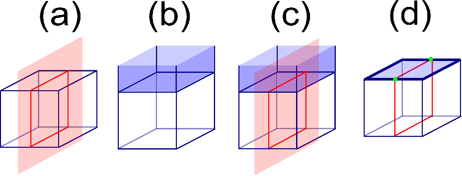
We begin with . To define the value of for some , consider the intersection between the set of red membranes and the cube . This intersection defines a collection of closed loops that live on the surface of the cube (Fig. 4a). (The fact that the loops are closed follows from the closed membrane constraint ). We will call these loops “red loops.” The integer is defined to be the number of these red loops, i.e.,
| (16) |
(See Fig. 4d for an example).
To define the value of for some , consider the intersection between the set of blue membranes and the cube . Because the blue membranes and the cube both live on the same cubic lattice, the intersection consists of 2D regions instead of loops. These 2D regions live on the surface of the cube (Fig. 4b). Consider the boundary of these 2D regions. This boundary consists of a collection of closed loops. We will call these loops “blue loops.” The integer is defined to be the number of intersections between the blue loops and the red loops defined above:
| (17) |
(See Fig. 4d for an example). Notice that is always even.
The integers and are defined in an identical way but with the colors reversed:
| (18) |
and
| (19) |
Here, the blue loops are defined by the intersection between the blue membranes and the red cube , while the red loops are the boundaries of the intersections between the red membranes and the cube .

Alternatively, we can express in the spin language. In this language, the operator can be written as a function of the twelve spins that are closest to (Fig. 5a), and similarly for :
| (20) |
Here is a finite polynomial, but the explicit form of is not illuminating so we do not show it here. Likewise, we can write as a function of the blue spins and red spins, surrounding the cube (Fig. 5b), and similarly for :
| (21) |
As above, the expression for is complicated so we do not show it here.
While the Hamiltonian is essentially identical to the well-known 3D toric code model[21, 24, 23, 25], some readers may be curious about the origin of the Hamiltonian . As we mentioned previously, this Hamiltonian has been designed to have a particular ground state — namely, . The state is in turn motivated by the ground state of the spin model in Ref. 27 which describes a nontrivial symmetry-protected topological phase with symmetry. Thus, the main question is how to design an exactly soluble Hamiltonian with a particular ground state, . One way to do this is to follow a similar approach to the string-net construction of Ref. 23. We recall that the string-net models of Ref. 23 can written as a sum of two types of operators — a operator and a operator. The operator prefers closed string configurations and the operator creates a closed loop. While the form of the operator is simple and intuitive, the operator is more complicated, and its matrix elements are obtained by fusing a closed loop onto the lattice using 2D local rules. The Hamiltonian can be constructed using a similar approach: in this case the Hamiltonian is built out of operators which prefer closed membrane configurations and operators which create a cube. Similarly to the string-net models, the precise form of the operator can be obtained by writing down local rules obeyed by , and then fusing a cube onto the lattice using 3D local rules. This is one way to obtain . Another way is to use membrane operators: as we will see in section III.3.4, the are examples of spherical membrane operators (35,38).
II.5 Properties of the Hamiltonians
The two Hamiltonians have many nice properties. One property is that all the operators are Hermitian so that and are also Hermitian. Indeed, the Hermiticity of is clear from the definitions (9,10), while the Hermiticity of and can be seen by noting that the matrix elements of and , as defined in (15), are both symmetric and real.
Another important property is that all the terms in commute with one another, so that the two models are exactly soluble. For the case of , the fact that all commute with one another follows easily from the definitions (9,10) of these operators. For the case of , more work is required to verify this commutativity: while simple algebra shows that
| (22) |
and
the fact that
| (24) |
is not obvious. We leave the derivation of the latter identity (24) to Appendix A.
A third property of is that the operators have eigenvalues or :
| (25) |
(The first two eigenvalue spectra can be derived from , etc.). A final property of these models is that is an simultaneous eigenstate of with
| (26) |
Similarly, is a simultaneous eigenstate of with
| (27) |
A derivation of the relations (26) and (27) is given in Appendix A.
II.6 Solving the models
In this section, we show that and are gapped, and that and are ground states of these Hamiltonians. We begin with . To find the energy spectrum of , recall that the operators commute with one another and can therefore be simultaneously diagonalized. Let us label these simultaneous eigenstates by where denote the eigenvalues. It is clear that these states are energy eigenstates with energy
| (28) |
Now, since the eigenvalues take values in , it follows that the ground state(s) of have , while the excited states have at least one equal to . We conclude that there is a finite energy gap, , separating the ground state(s) and excited states. Furthermore, we can see that is a ground state of since it obeys (26). All that remains is to determine the ground state degeneracy of . This degeneracy depends on the global topology of the system on which is defined. In an infinite non-periodic geometry, one can show that has a unique ground state — namely, . On the other hand, in periodic (3D torus) geometry, it can be shown that the ground state degeneracy is . These degenerate ground states are characterized by different parities of noncontractible red and blue membranes along the and directions of the 3D torus.
Now let us consider Hamiltonian . Similarly to , we can simultaneously diagonalize and label their eigenstates as . Following the same reasoning as above, we conclude that there is a finite energy gap, , separating the ground state(s) and excited states. Furthermore, we can see that is a ground state of since it obeys (27). Like , it can be shown that has a unique ground state in an infinite non-periodic geometry (), and the ground state degeneracy is in a 3D torus geometry.
II.7 Particle-like and loop-like excitations
If we examine equation (28), we can see that supports both particle-like and loop-like excitations. An example of a particle-like excitation is a point defect where or is equal to instead of the ground state value of . Likewise, an example of a loop-like excitation is a line defect along which or is equal to instead of the ground state value of . These line-like defects always form closed loops: to see this, note that the quantum numbers and obey the local constraints
| (29) |
for every site in the cubic lattice and in the dual cubic lattice. Here, the first product runs over the six edges that are adjacent to and similarly for the second product. The above constraints guarantee that each site is adjacent to an even number of line-line defects, so that the defects always form closed loops. (To derive these constraints, note that they follow from the corresponding operator identities, which in turn follow from the definition (9)). In exactly the same way, one can see that the Hamiltonian supports particle-like excitations with or is equal to , and loop-like excitations where or is equal to along some closed loop.
Below we will see that in both models, these particle-like and loop-like excitations have nontrivial braiding statistics with one another and have similar properties to the charges and vortex loops in gauge theories. In view of this connection, we will refer to the particle-like excitations with or equal to as “blue charges” and the excitations with or equal to as “red charges.” Similarly, we will refer to the loop-like excitations with as “blue vortex loops” and the excitations with as “red vortex loops.” In the following, we will study these charge and vortex-loop excitations in more detail, with a focus on their topological properties.
III Excitations and the associated creation operators
In this section, we find operators that create the charge and vortex loop excitations of and . These operators are useful because their commutation algebra contains information about the braiding statistics of the associated particles and loops.
III.1 General picture for string and membrane operators
In general, topologically nontrivial particle excitations cannot be created using local operators. Instead, the easiest way to create these excitations is to use string-like operators. In the following sections we will find string-like creation operators for each topologically distinct charge excitation in and . We will denote these operators by where is the path along which the string operator acts. These operators satisfy two key properties. First, if is an open path, then when is applied to the ground state , it creates an excited state with two charge excitations at the two ends of :
(Here the excited state only depends on the endpoints of and not on the choice of path). Second, if is a closed path, then does not create any excitation at all: .
In addition to these string operators, which create charge excitations, we will also find membrane operators that create vortex loop excitations. That is, for each topologically distinct vortex loop excitation in and , we will find a corresponding membrane creation operator, which we will denote by with being the surface where the membrane operator acts. These membrane operators satisfy similar properties to the string operators. First, if is a cylindrical surface, then when is applied to the ground state it creates an excited state with two loop excitations at the ends of the cylinder:
(Similarly to before, the excited state only depends on the two boundaries of and not on the choice of surface that joins them). Second, if is a toroidal surface, then does not create any loop excitations at all: .
We can also consider membrane operators with other topologies beyond the cylinder and torus case: for example, later we will discuss spherical membrane operators. However, the structure of membrane operators is different for different topologies44 4 For example, toroidal operators can be decorated by string operators that encircle the torus while spherical membrane operators cannot be decorated in this way. See section III.3.4 for more details. and thus each case has to be treated separately. Here we will focus on cylindrical and toroidal cases as they are sufficient for our purposes.
The string and membrane operators have simple physical interpretations: the string operator describes a process in which a pair of charge excitations is created and then moved to the two ends of the path . Likewise, the membrane operator describes a process in which a pair of loops is created and then moved to the two ends of the cylinder . On the other hand, if is a closed path then describes a process in which a pair of charge excitations is created and then moved around and annihilated with each other. Similarly, if is a toroidal surface then describes a process in which a loop-antiloop pair is created, moved around and annihilated with one another.
III.2 String and membrane operators for
III.2.1 String operators
It is easy to find string operators , that create the blue and red charge excitations of . These operators are given by
| (30) |
where is a path on the dual cubic lattice in the first expression, and a path in the cubic lattice in the second expression. The two products run over plaquettes that are perpendicular to these two paths. Equivalently, in the membrane representation, and are given by:
| (31) |
where and are the number of blue and red membranes that cross the path .
Let us now verify that when is an open path, creates blue charge excitations at the two endpoints of . From the definitions (30), it is easy to see that commutes with all the terms in the Hamiltonian except for and where and are the two cubes at the endpoints of . These two operators anticommute with rather than commute. We conclude that is a simultaneous eigenstate of with eigenvalues and all other eigenvalues equal to . Hence, contains two blue charge excitations at the endpoints of . A similar argument shows that also creates red charge excitations at the endpoints of .
III.2.2 Membrane operators
It is also easy to find membrane operators , that create the blue and red vortex excitations of . These operators are given by
| (32) |
where is a surface made up of plaquettes living in the cubic lattice in the first expression, and a surface consisting of plaquettes in the dual cubic lattice in the second expression. Equivalently, we can express and in the membrane representation as:
| (33) |
where denotes the addition operation defined below equation (8).
We now check that when is a cylindrical surface, creates blue loop excitations at the two ends of . To establish this fact, we note that commutes with all the terms in the Hamiltonian except for when lies along the two boundaries of . These operators anticommute with rather than commute. It then follows that is an eigenstate of with eigenvalues along the boundaries of , and all other eigenvalues equal to . This establishes the claim. The same argument applies to .
It should be noted that the excitations created by and are not the most general possible vortex loop excitations. In fact, the model supports three other types of blue vortex loops and three other types of red vortex loops. These excitations can be obtained by attaching either a red charge, a blue charge, or both a red charge and a blue charge, to the vortex loops created by and . We will label the four types of blue vortex loops by , and the four types of red vortex loops by where take values in . In this labeling scheme, the excitations created by and are denoted by and , with the other excitations labeled according to the amount of charge attached to them. As we will see later, these loop excitations are all topologically distinct from one another in the sense that they have different braiding statistics.
It is easy to find membrane operators that create these more general vortex loop excitations. For example, consider the operator in the case where is a cylinder. When this operator is applied to the ground state , it creates two vortex loops of type at the two ends of the cylinder. We can modify this operator to create other vortex loops by multiplying by the string operators or or where the paths run along the length of the cylinder. In the same way, we can construct membrane creation operators for the red vortex loops by multiplying by appropriate string operators.
Before concluding, we should mention that there is yet another type of vortex loop excitation which we have not discussed, namely a composite of a red and blue vortex loop. This type of loop excitation can be obtained by fusing together a red and blue loop, and again it comes in four subtypes which we can denote by . In what follows, we will generally ignore this additional kind of vortex loop excitation since its braiding statistics properties are completely determined by the properties of the individual red and blue loops.
III.3 String and membrane operators for
In this section, we construct string and membrane operators for the Hamiltonian . The string operators are relatively easy: following the same analysis as above, it is simple to check that the same string operators that create the blue and red charge excitations in the model can also be used to create the charge excitations in the model. That is, just as in (31), we can set
| (34) |
where and are the number of blue and red membranes that cross the path .
We will need to do more work to construct membrane operators for . The rest of this section is devoted to this problem.
III.3.1 Cylindrical membrane operators for blue vortex loops
We begin by finding a membrane operator that creates blue vortex loops. To proceed, it is convenient to work in the membrane basis. Let be a cylindrical surface made up of plaquettes living in the cubic lattice. We need to define the action of on a general membrane state . A natural guess, inspired by (33), is that should act as
| (35) |
for some complex-valued function . Indeed, it is easy to see that any operator of this type has the property that it anticommutes with the terms that lie along the two boundaries of and it commutes with every other and term. Hence, any operator of this type has the property that if we apply it to the ground state , it will create blue vortex loop excitations at the boundaries of . The problem is that most of these operators also create many other excitations along the surface since most of these operators do not commute with and . Thus, our task is to choose appropriately so that does not create any excitations except at the boundaries of .
We now describe one choice of that does the job. Below, we will just present the definition of without any motivation. Later, in section III.3.5, we will explain why this choice works and we will provide some motivation as to where it comes from.
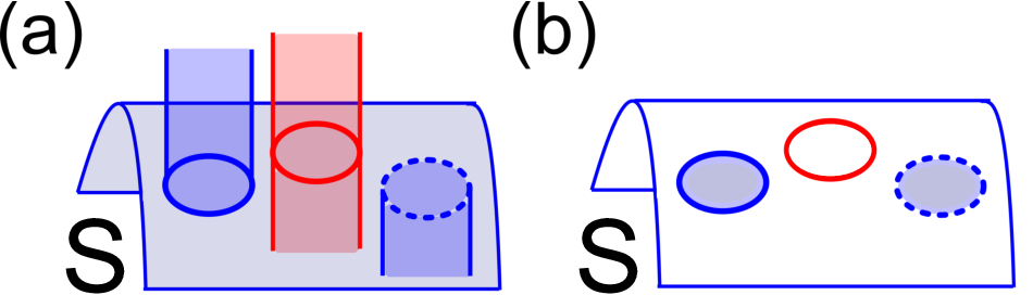
First, we set if the membrane configuration violates the closed membrane constraint anywhere in the neighborhood of . More precisely, if any link that touches or intersects is adjacent to an odd number of occupied plaquettes. On the other hand, if every such link is adjacent to an even number of occupied plaquettes, then is defined in terms of the two intersections and . The dependence of on and is complicated, and in order to explain it, we first describe a way to represent and as a picture drawn on the surface of the cylinder . The picture we will draw consists of a collection of red lines and blue regions with the red lines denoting the places where membranes in intersect , and the blue regions denoting the places where membranes in intersect/overlap with . We note that the boundaries of the blue regions correspond to places where a membrane in is incident upon the surface . If this membrane is incident upon from above, we will draw the corresponding boundary as a solid line, while if it is incident from below, we will draw the boundary as a dotted line (Fig. 6). (Note that for this step to be well-defined, one needs to specify a convention for what side of is defined as “above” and what side is defined as “below” . Equivalently, one needs to choose a normal vector to ). Putting this all together, the intersections and can be represented by a picture, drawn on the cylinder , of the form shown in Fig. 7.

The value of is completely determined by the corresponding picture. Thus, can be thought of as a complex-valued function defined on pictures. All that remains is to specify this function. For reasons that will become clear later on, it is most natural to describe implicitly, through local constraint equations, rather than providing an explicit formula. More specifically, we define in terms of the constraint equations
| (36a) | ||||
| (36b) | ||||
| (36c) | ||||
| (36d) | ||||
| (36e) | ||||
| (36f) | ||||
| (36g) | ||||
| (36h) | ||||
| (36i) | ||||
| (36j) | ||||
where it is understood that the value of depends only on the topology of the picture. That is, any two pictures that can be smoothly deformed into one another have the same value of . The meaning of the above constraint equations is as follows. The first equation (36a) states that the value of for a picture with a closed red loop is equal to the value of for the same picture, without the loop, up to a factor of . Equation (36b) states that two pictures that differ by the recoupling of red curves have values of that differ by a factor of . The remaining equations have a similar meaning.
In the above constraint equations, we have left out the shading of the blue regions. But it should be understood that the blue regions are shaded in a consistent way on both sides of the equations. For example, (36d) represents two constraints with different shadings
Similarly, (36j) also represents two constraints with different shadings
![[Uncaptioned image]](1503.00142v2/p0.png) |
![[Uncaptioned image]](1503.00142v2/p1a.png) |
![[Uncaptioned image]](1503.00142v2/p1b.png) |
![[Uncaptioned image]](1503.00142v2/p1c.png) |
![[Uncaptioned image]](1503.00142v2/p1d.png) |
|---|---|---|---|---|
To complete the definition, we impose a boundary condition on which states that if any of the red lines or blue regions touch the boundaries of . With this boundary condition and the above constraint equations, the value of on any picture can be related to one of the four “basic” pictures shown in Table 1. Thus, once we specify the value of on these basic pictures, we will have completely specified and therefore .
The values for on the basic pictures are shown in the bottom row of Table 1. These values are parameterized by two integers . Hence our construction actually defines four different membrane operators. In principle, we should label these operators by to make the dependence on explicit. However, this notation is cumbersome so we will denote the membrane operators by with the understanding that is not fully defined until we specify . Similarly to the model, these four different blue membrane operators create four different types of blue vortex loops. These vortex loops differ from one another by the amount of charge that they carry and we will label them by .
At this point, we have fully defined the membrane operator . All that remains is to show that this membrane operator has the required properties. That is, we need to show that creates blue vortex loops at its two boundaries and nothing else. We will establish this fact in section III.3.5.
III.3.2 Cylindrical membrane operators for red vortex loops
To construct cylindrical membrane operators that create red vortex loops, we follow exactly the same recipe as above but with the roles of “red” and “blue” reversed. First, we define
| (37) |
where is a complex-valued function. We then define in terms of the two intersecting sets and . As in the definition of , we represent and in terms of a picture drawn on the surface of the cylinder , and we think of as a function defined on such pictures. In this case, each picture consists of a collection of blue lines and red regions, where the blue lines denote the intersection , and the red regions denote the intersection . We define the value of on each picture using local constraint equations which are identical to Eqs. (36), but with the red and blue colors reversed. With these constraint equations, the value of on any picture can be related to one of the four basic pictures shown in Table 1 (with the colors reversed). We then define the value of on these basic pictures, just as in Table 1 but with the colors reversed and and exchanged. This procedure completely specifies and therefore . Note that, like , this construction actually gives four different membrane operators that are parameterized by two integers . These membrane operators create four different types of red vortex loops, which we denote by .
III.3.3 Cylindrical membrane operators for linked loops
We now have all the tools we need to create an excited state with a pair of vortex loops: to do this we simply apply one of the above cylindrical operators to the ground state . But what if we want to build a state with more than two vortex loops? One might try to make such a state by applying multiple cylinder operators to the ground state. This approach will work fine if the state we are trying to build does not contain any linked loops. However, it will fail if any of the loops are linked: the above membrane operators are simply incapable of creating excited states with linked loops. To see this, imagine we first apply a cylindrical membrane operator to the ground state, obtaining . This state contains two blue vortex loop excitations located at the two boundaries of the cylinder . Now, suppose we apply another cylinder operator where is linked with one of these loops. One might hope that the result would be a state with linked vortex loops. Unfortunately, however, simply annihilates this state: . To see this, note that is a superposition of membrane states , where all the membranes in and form closed surfaces, except at the two boundaries of , where a blue membrane terminates. Since is linked with one of the boundaries of , it follows that each of the two boundaries of must intersect with blue membranes an odd number of times. In particular, each boundary must have at least one intersection with a blue membrane. But if we look back at the boundary conditions for , we see that any state of this kind has , so any state of this kind is annihilated by .
We therefore need to find another set of membrane operators to create linked loops. We now define such membrane operators. Before doing this, we first need to explain the basic idea behind these operators. In general, we will be interested in excited states containing a collection of vortex loops that are all linked with a single “base loop” which can be either blue or red. We will build such states with the help of two different cylindrical membrane operators — one for each type of base loop. The operator associated with the blue base is designed to be applied to states containing a blue loop that links with the cylinder : when the operator is applied to such a state, it creates two vortex loops at the ends of the cylinder which are linked with the original blue loop. On the other hand, when it is applied to states that do not contain a blue loop that links with the cylinder , it simply annihilates them. The operator associated with the red base has a similar property. This structure is reminiscent of the cylinder operators constructed in the previous two sections. In fact, the previously constructed operators can be thought of as cylindrical membrane operators associated with a trivial base: they only create loop excitations when applied to states without any loops linked with .

With this picture in mind, we now construct cylindrical membrane operators for a red base loop and a blue base loop. We begin by defining a cylindrical membrane operator that creates blue vortex loops that are linked to a red base loop. This operator is defined in almost exactly the same way as the blue membrane operator defined above. The only difference is that we change the boundary condition on so that it only takes nonzero values on pictures in which a single red line touches the boundary of at a fixed position , and no blue regions touch the boundary. (See Fig. 8a for a typical picture of this type). Given this boundary condition and the constraint equations (36) we can reduce any such picture to one of the four basic pictures shown in the top panel of Table 2. We can therefore completely specify the membrane operator once we specify the value of on these four basic pictures. The values we choose are shown in Table 2.
![[Uncaptioned image]](1503.00142v2/p0r.png) |
![[Uncaptioned image]](1503.00142v2/p2a.png) |
![[Uncaptioned image]](1503.00142v2/p2b.png) |
![[Uncaptioned image]](1503.00142v2/p2c.png) |
![[Uncaptioned image]](1503.00142v2/p2d.png) |
|---|---|---|---|---|
![[Uncaptioned image]](1503.00142v2/p0b.png) |
![[Uncaptioned image]](1503.00142v2/p3a.png) |
![[Uncaptioned image]](1503.00142v2/p3b.png) |
![[Uncaptioned image]](1503.00142v2/p3c.png) |
![[Uncaptioned image]](1503.00142v2/p3d.png) |
We next describe a cylindrical membrane operator which creates a blue vortex loop which is linked to a blue base loop. Here, we choose a boundary condition on so that it only takes nonzero values on pictures in which a single thin blue region touches the boundary of at a fixed position , and no red lines touch the boundary. (See Fig. 8b for a typical picture of this type). Given this boundary condition and the constraint equations (36), we can reduce any such picture to one of the four pictures shown in the bottom panel of Table 2. The value of on these four pictures is shown in Table 2.
To complete the discussion, we need to explain how to construct cylindrical membrane operators that create red vortex loops linked to a blue or red base loop. These operators are defined exactly like the two operators described above, but with the roles of “red” and “blue” reversed.
Before concluding, we make one comment about our notation: we will use the same symbol to denote all of the blue membrane operators whether they are associated with a red base (top panel of Table 2), a blue base (bottom panel of Table 2), or no base at all (Table 1). Similarly, we will denote all the red membrane operators by independent of what base they are associated with. This abuse of notation will not introduce confusion since it will always be clear from context which operator we have in mind.
III.3.4 Toroidal and spherical membrane operators
So far we have only discussed cylindrical membrane operators. We now discuss how to construct membrane operators with other topologies — in particular, toroidal and spherical operators. We begin with the toroidal operators. Roughly speaking, these operators can be obtained by connecting the two ends of our cylinder operators. More precisely, we define toroidal operators exactly like the cylindrical operators, with only one modification: we replace the cylindrical boundary conditions on and with periodic boundary conditions in both directions of the torus.
Like cylindrical operators, we can build different torus operators for different base loops. The blue torus operator for a trivial base loop is defined by the values of shown in Table 1 while the blue torus operator for a red base loop is defined by the values shown in the top panel of Table 2. Finally, the blue torus operator for a blue base loop is defined by the values of shown in the bottom panel of Table 2. Red torus operators for various base loops can be defined in the same way but with the red and blue colors exchanged.
It is important to keep in mind that the two coordinates that describe the torus are not equivalent. One coordinate parameterizes the movement of the loop in space, while the other coordinate parameterizes the loop itself. Thus to define a torus operator, we not only have to specify the torus , but we also have to specify which coordinate has which meaning.
Let us now discuss spherical membrane operators. We can define blue spherical operators following the same recipe as the blue cylindrical operators. The only difference is that in the spherical topology, every picture can be reduced to the vacuum or (empty) picture by application of the constraints (36) — in contrast with the cylindrical case where every picture can be reduced to one of the four pictures shown in Table 1 or Table 2. Thus, in the spherical case it suffices to define the value of on the vacuum picture. Here we define . Note that there is only one type of blue spherical operator — unlike the cylindrical or toroidal case where there are four types of operators parameterized by .
In fact, we already encountered spherical membrane operators in the definition of the Hamiltonian : the operators and (15) can be thought of small spherical membrane operators associated with a unit blue cube or unit red cube . To see that is a spherical membrane operator, note that the picture drawn on the surface of the blue unit cube has the property that the boundaries of the blue regions are always solid lines —that is, there are no boundaries that are dotted lines. The reason this is so is that all membranes in are incident on the cube from the outside, rather than the inside. Now, since the picture on the surface of the cube does not contain any dotted blue lines, the local constraints (36) simplify considerably: in fact, we can throw out equations (36e) - (36g) and (36i-36j). The resulting equations can be solved explicitly, leading to the following formula for :
| #{red loops on } | ||||
| (38) |
We can see that this formula, together with the definition (35) agrees exactly with the definition of .
III.3.5 Showing that the membrane operators have the required properties
Having defined the membrane operators and , we now show that they have the required properties. We will focus on one case, namely blue membrane operators that create unlinked loop excitations. The arguments for the linked case are similar.
To begin, we show that if is a torus then does not create any excitations at all. That is, we show
| (39) |
To establish this result, we first rewrite (39) in a more convenient form. Multiplying both sides by gives:
| (40) |
Next, using the definition of (35), we can rewrite this as
| (41) |
To proceed further, we observe that Eq. (41) is equivalent to the relation
| (42) |
for any two closed membrane configurations and . Finally, we use the fact that is a pure phase to rewrite this equation as
| (43) |
Our task is now to prove equation (43). First, we claim that it suffices to prove (43) for the case where and only differ locally — i.e. only differ in some small region. The reason it is enough to consider this case is that we can get from any membrane configuration to any other configuration by a series of local changes:
If (43) holds for each pair , then once we multiply these relations together, we see that it automatically holds for and .
There are two cases to consider: the region where and differ may overlap or not overlap . In the second case, it is easy to see that (43) holds. Indeed, in this case the left hand side of (43) is equal to since only depends on the membrane configuration in the neighborhood of and hence . Similarly, the right hand side of (43) is also equal to since the ratio only depends on the membrane configuration in the region where and differ from one another.

All that remains is the case where and differ in a small region that overlaps . In this case, the ratio on the left hand side of (43) is directly determined by the local constraint equations (36) for . The key point is that these constraint equations were chosen specifically so that a solution to these equations will automatically obey (43). This is easiest to see by example. Consider a blue torus operator acting on the two configurations and shown in Fig. 9. Here consists of a single blue sphere, while consists of two red spheres and consists of single red sphere obtained by merging together the two spheres in . In this case
so that
| (44) |
according to (36b). On the other hand, it is easy to see that
using the explicit formula for (2). We conclude that
| (45) |
so that equation (43) is satisfied in this case.
The above example serves two purposes. First it demonstrates, in at least one case, that obeys equation (43). Second, it reveals where the constraint equation (36b) comes from: it should be clear that we chose the factor of in this equation specifically to ensure that (43) was satisfied. Similarly, one can check that the other constraint equations (36) ensure that obeys (43) in other cases.
This concludes our argument showing that the torus operator does not create any excitations when applied to the ground state. Next, we need to show that the cylinder operator does not create any excitations except at the two boundaries of . This claim can be established using a similar argument to the torus case, but we will not repeat the derivation here. Instead we simply observe that the cylinder and torus operators look identical except near the two boundaries of the cylinder. Therefore it is intuitively clear that since the torus operator does not create any excitations, the same must be true of the cylinder operator away from its boundaries.
At this point, we have argued that the cylinder operator creates blue loop excitations at its two boundaries and no other excitations anywhere else. However, we are not quite finished: we still need to verify one more property of the cylinder operator . Recall that supports four topologically distinct types of blue loop excitations which differ from one another by attaching red and blue charges (see section III.2.2). We need to check that creates exactly one of these excitations, and not a linear superposition of different types of excitations. In other words, we need to check that creates loop excitations that are eigenstates of braiding measurements.
To see that creates braiding eigenstates, we make use of a result from appendix B. In that appendix, we show that the cylinder operators are guaranteed to create braiding measurement eigenstates provided that is multiplicative in the sense that
| (46) |
for any two cylinders and that share a common boundary and any membrane configuration whose intersection with the common boundary obeys the appropriate cylinder operator boundary condition.
In view of this result, we only have to show that obeys condition (46). We go through this calculation in appendix B, and we show that does indeed obey (46) provided that the values of on the four basic pictures are those shown in Table 1. In fact, this is why we picked the particular values shown in that table: we chose those values to ensure that obeys equation (46).
To summarize, we have shown that the cylinder operators create blue loop excitations at their two boundaries and no other excitations anywhere else. We have also shown that these blue loop excitations are eigenstates of braiding measurements. This establishes that the cylinder operators have all the required properties.
III.4 Labeling scheme for loop excitations
In this section, we discuss some subtleties related to the labeling of loop excitations. As we have emphasized previously, both the and models support four different kinds of blue loop excitations and four different kinds of red loop excitations. We label the former by and the latter by where . In practice, we first assign labels to the membrane operators; we then assign labels to the loop excitations according to which membrane operator creates them.
Now, an important question is how we choose which loop excitations are labeled by and . We will call these excitations neutral loops. Once we decide which blue and red loops should called neutral, the labeling of all the other excitations is naturally fixed: for example, we assign the label to the loop that is obtained by attaching blue charge and red charge to the neutral loop, .
For the case of unlinked loops, there is a natural choice for which loop should be called neutral: the neutral loop is the unique loop that can be shrunk down to a point and annihilated by a local operator. Thus, for the case of unlinked loops there is a canonical labeling scheme. This is the labeling scheme we use here. Indeed, in the case of , we assign to the loop created by the operator (32), and one can readily verify that this loop is the unique blue loop that can be annihilated locally. Similarly, in the case of , we assign to the loop created by the membrane operator defined in Table 1 with and one can also check that this loop can be annihilated locally. (One way to see this is to note that if we shrink the two ends of the cylinder to make a sphere, the operator defined by Table 1 reduces to the spherical membrane operator defined by (38)).
In contrast, for linked loops, there is no canonical way to define which loops are neutral. Therefore, we make this assignment arbitrarily. In other words, for each base loop, we arbitrarily choose one of the blue linked loops and one of the red linked loops, and we call them neutral. In the case of , this arbitrary choice enters in how we parameterize the values in Table 2 which define the membrane operators and hence define the loop excitations. As we show in appendix B, the values in Table 2 are obtained by solving certain algebraic equations. These equations have four different solutions, which define four different membrane operators. All four are on an equal footing, but we simply picked one and labeled it by . The labeling of the other solutions is then completely fixed. We could replace or , for either the top or bottom panel of Table 2, and the resulting table would define an equally valid labeling convention.
The arbitrariness of our labeling scheme has an important consequence: because we picked the labels in an arbitrary way, there is no sense in which an unlinked loop of type is the “same” type as a linked loop of type . More generally, we cannot sensibly compare loops that are linked with different base loops. Each base loop effectively defines its own universe of excitations.
IV Braiding statistics of excitations
In the previous section, we constructed operators that create charges and vortex loops for the models. In this section, we will use these operators to compute the braiding statistics of these excitations. We consider four types of processes: (1) processes involving two charges, (2) processes involving a charge and a vortex loop, (3) processes involving two vortex loops, and finally (4) “three-loop processes” involving two vortex loops that are both linked with a third loop. We find that the two models have the same braiding statistics except for the last process; when we investigate the three-loop braiding process we find a distinction between the two models which implies that they belong to distinct topological phases.
IV.1 Braiding two charges

To compute the statistics of the charge excitations, we use the “hopping operator algebra” derived in Ref. 22. This algebra relates the exchange statistics of particle excitations to the commutation properties of the string operators that create these particles. To see how this works, let us consider the blue charge excitations in the model. According to the hopping operator algebra, the exchange statistics of these excitations can be read off from the phase factor in the commutation relation
| (47) |
where are three paths arranged in the geometry of Fig. 10 and is the ground state of . That is, if , then the blue charges are bosons, while if , the blue charges are fermions. (Other values of are not possible in 3D). If we examine the form of the string operators, we can see that since the string operators (30) all commute with one another. We conclude that the blue charges are bosons in the model. Using identical reasoning, we can see that the blue and red charges are bosons in both models.
IV.2 Braiding a charge and a vortex loop

Next, we compute the statistical Berry phase associated with braiding a charge around a vortex loop. More specifically, let us consider the model and imagine braiding a blue charge around a blue vortex loop. The statistical phase for such a process can be read off from the commutation algebra of the corresponding string operator and membrane operator
| (48) |
where is a closed path and is a cylindrical surface, arranged as in Fig. 11a. To see where this relation comes from, note that the operator describes a process in which two vortex loops are created and moved to the ends of the cylinder , while the operator describes a three-step process in which two charges are created out of the vacuum, one of them is braided around the path , and then the two annihilated with one another. With this interpretation, the right hand side of (48) describes a process in which two vortex loops are created and then a charge is braided around , while the left hand side describes a process in which a charge is braided around first, and then two vortex loops are created. Clearly the phase difference between these two processes is the statistical phase associated with braiding a charge around a vortex loop.
Remembering the definition of and , we can see that these operators anticommute with each other. We conclude that braiding a blue charge around a blue vortex loop results in a statistical phase of . Similarly, we can see that and anticommute with each other so braiding a red charge around a red vortex loop gives a phase of . On the other hand, if one braids a red charge around a blue vortex loop or a blue charge around a red vortex loop, the statistical phase vanishes since these operators commute with one another.
A similar calculation for the model gives identical results. Thus the two models share the same statistics between charges and vortex loops. We note that these statistical phases agree with the Aharonov-Bohm phases associated with braiding a charge around a vortex loop in gauge theory. This is not a coincidence: as we mentioned in the introduction, the two models can be viewed as two different types of gauge theories.
IV.3 Braiding two vortex loops
IV.3.1
We now consider, for the model, the statistical phase associated with braiding a vortex loop around another vortex loop (Fig. 1a). For example, let us consider braiding a blue vortex loop around another blue vortex loop. Similarly to Eq. (48), the statistical phase can be computed from the commutation relation
| (49) |
where is a cylinder and is a torus, arranged as in Fig. 11b. Examining the definition of the membrane operators (32), we can see that they commute with one another so that . Likewise, we can see that there is no statistical phase associated with braiding a red loop around a red loop or a red loop around a blue loop since the corresponding membrane operators all commute with one another.
The above results apply to the blue vortex loop and red vortex loops labeled by and . One might also wonder about the braiding statistics of more general vortex loops and . The braiding statistics of these more general vortex loops can be computed using the same approach as above. The only difference is that the membrane creation operators are slightly different in this case: they are obtained by multiplying (or ) by one of the string operators , or , where the paths run along the length of the cylinder. Substituting these modified membrane operators into Eq. (49), a simple calculation shows that the phase associated with braiding a blue vortex loop around another blue vortex loop is given by
| (50) |
Similarly, the phase associated with braiding a red vortex loop around another red vortex loop is
| (51) |
while the phase associated with braiding a red vortex loop around a blue vortex loop is
| (52) |
These expressions have a natural interpretation in terms of Aharonov-Bohm phases: the first term in each formula is the statistical phase associated with braiding the charge on the first vortex loop around the flux of the second loop while the second term is the phase associated with braiding the flux of the first vortex loop around the charge on the second loop.
IV.3.2
Similarly to the case, the statistical phase associated with braiding a blue vortex loop around a blue vortex loop in the model can be read off from the commutation algebra of the corresponding membrane operators:
| (53) |
However the membrane operators are more complicated than their counterparts in the model, so it is more difficult to apply Eq. (53). To deal with this issue, we now derive a simpler version of Eq. (53) which is more convenient for our purposes. The first step is to rewrite Eq. (53) as
where . Next, we use the fact that , which implies that all of the states that appear in the above sum are linearly independent from one another. It follows that the above equality must hold for each term separately. Hence, we must have
| (54) |
for every membrane state that has a nonzero amplitude in the state .
We will now use (54) to compute the statistics of the loops in the model. To this end, we set , the “no-membrane” state. We then define , , and . With this notation, the left side of (54) can be computed as
| (55) | |||||
Similarly, the term on the right side is given by
| (56) | |||||
Comparing these two expressions with (54), we derive
| (57) |
To complete the calculation, we compute the value of for each of these configurations
| (58) |
Substituting these values into (57), we find that the statistical phase associated with braiding a loop around another loop is
| (59) |
We note that this result is identical to the statistical phase (50) in the model. Similarly, it is easy to check that the phase associated with braiding two red loops around one another agrees with (51) while the phase associated with braiding a red loop around a blue loop agrees with (52). Thus, the two models share the same two-loop braiding statistics. In fact the agreement between the two models is not surprising, since the two models are equivalent to gauge theories, and in such systems the two-loop braiding statistics always has an Aharonov-Bohm form, as explained in Ref. 14.
IV.4 Three-loop braiding
Finally, we discuss the three-loop braiding statistics in the two models. Specifically, we consider a braiding process in which a loop is braided around another loop, while both are linked to a third “base” loop (Fig. 1b). Unlike the other processes we have considered until now, we will see that the two models can be distinguished by their three-loop statistics.
IV.4.1

First we compute the statistics in the model. As in the two-loop case, the three-loop braiding statistics can be read off from the commutation algebra for the membrane operators. For example, the statistical phase associated with braiding a blue vortex loop around a blue vortex loop, while both are linked to a red base loop can be obtained from
| (60) |
where is a cylinder, is a torus, and is an excited state with a red vortex loop that links with both and (Fig. 12). Remembering that the membrane operators all commute with each other, we deduce that . In the same way, we can see that .
In the above calculation we implicitly assumed loops of the form . If we instead consider a process in which a general vortex loop is braided around another loop with either a red base loop or a blue base loop, then, just as in the two-loop case (50), one finds
| (61) |
Similarly, if we braid a red loop around another red loop with either base, the statistical phase is
| (62) |
Finally, braiding a red loop around a blue loop with either base gives the phase
| (63) |
The agreement with the two-loop statistics (50-52) is to be expected since the membrane operators , obey the same commutation algebra independent of whether they act on the ground state (as in the two loop case) or an excited state (as in the three loop case).
IV.4.2
We begin by computing the statistical phase associated with braiding a blue vortex loop around another blue vortex loop, while both are linked with a red base loop. As in the case, the statistical phase is given by
| (64) |
where is a cylinder, is a torus, and is an excited state with a red vortex loop that links with both and (Fig. 12). Following the same logic as in section IV.3.2, it is straightforward to deduce an alternative and more convenient form of equation (64):
| (65) |
where is any membrane state that has nonzero overlap with . To compute , we set where is a disk with a boundary along the red vortex loop. We then define , , and . With this notation, the left hand side of (65) can be computed as
| (66) |
while the expression on the right hand side can be written as
| (67) |
The three-loop statistics is then given by
| (68) |
To complete the calculation, we need to compute the values of on each of these configurations. We have
| (69) |
where the ‘’ sign in the last equation comes from using the local rules (36) to reduce the picture to one of the basic pictures in Table 2. Substituting these values into (68), we find that the statistical phase associated with braiding a loop around another loop while both are linked to a red base loop is given by:
| (70) |
In a similar manner, it is easy to show that the phase associated with braiding a red loop around another red loop , while both are linked to a red base is:
| (71) |
As another example, let us compute the phase associated with braiding a red loop around a blue loop, with a red base. The analogue of equation (65) in this case is
| (72) |
where is any state that has nonzero overlap with and is an excited state with a red vortex loop that links with both and . Letting , , , and , we derive
| (73) |
Proceeding as before, we find
| (74) |
Substituting these values into (73), we conclude that the statistical phase associated with braiding a loop around another loop while both are linked to a red base loop is
| (75) |
So far we have only discussed braiding processes involving a red base loop. We can find the braiding statistics associated with a blue base loop, by simply switching the roles of “red” and “blue”:
| (76) |
Putting together equations (70),(71),(75) and (76), we have found all the three-loop braiding statistics of the model. (Actually, one quantity that we have not computed is the exchange statistics of the loops. However, this quantity is not necessary for our purposes, since the mutual statistics computed above is sufficient to distinguish the two models).
Before concluding this section, we would like to mention that the three-loop statistics for appears to be identical to the three-loop statistics of one of the Dijkgraaf-Witten models[20, 36]. To see this, we follow the notation of Ref. 14, 18 and we summarize the three-loop statistics for in terms of the quantity where the indices , and is defined modulo . Translating equations (70),(71), (75) and (76) into the variables gives:
| (77) |
If we compare this data to the results of Ref. 14, we can see that it matches the three-loop statistics for the Dijkgraaf-Witten model labeled by . Based on this fact, we conjecture that belongs to the same phase as this Dijkgraaf-Witten model. 55 5 In fact, if our conjecture is correct then also belongs to the same phase as the Dijkgraaf-Witten models labeled by and , since the three Dijkgraaf-Witten models labeled by , and all belong to the same phase, when viewed as spin models rather than gauge theories.
IV.4.3 Comparing the three-loop statistics in the two models
With the above results, we now show that the and models have distinct three-loop statistics. To see an example of a difference between the two models, consider the formula for (75). This formula implies that, in the model, if we braid a red loop around a blue loop, while both are linked to a red loop the resulting phase is depending on what type of red and blue loops are being braided. In contrast, in the model, we can see from (61), (62), (63) that if we braid any two loops around one another, the resulting phase is always or , independent of the choice of base loop or what loops are being braided.
For another example of a difference, consider the formula for (70) for the case where the two blue loops , are identical, i.e. and . In this case, . This means that if we braid two identical blue loops around one another while they are both linked to a red loop, the resulting statistical phase is in the model. On the other hand, in the model, we can see from (61), (62), (63) that if we braid any two identical loops around one another the resulting phase is always , independent of which loops or base loops are involved.
From the above examples, it is clear that there is no way to map the loop excitations of onto the loop excitations of in such a way that the corresponding loops have the same statistics. Importantly, we can rule out all possible mappings between the two sets of loop excitations including those that change the “colors” or “charges” of the loop, e.g. that map the excitation in onto in . (This generality is important because the “colors” and “charges” of the loops have no physical meaning in this context except as a scheme for labeling excitations). We conclude that the two models have physically distinct three-loop statistics, and hence must belong to different phases.
V Conclusion
In this paper, we have presented an explicit computation of the three-loop braiding statistics of two spin models, . The key step in our analysis was our construction of membrane operators that create and move loop excitations. With the help of these operators, we were able to implement the three-loop braiding process on the lattice and find the associated statistical phase in each of the models. While technically complicated, this membrane operator approach has the advantage that it is more direct than previous calculations based on dimensional reduction[14] or modular transformations on a 3D torus.[15, 16] An additional feature of our results is that they provide a concrete demonstration of the utility of three-loop braiding statistics for distinguishing 3D gapped phases: indeed, we have shown that the two models and share the same particle exchange statistics and the same particle-loop and loop-loop braiding statistics. The only way to see that these models belong to distinct phases is to examine their three-loop braiding statistics.
The discussion in this paper raises an important question, namely whether three-loop braiding statistics, together with particle exchange statistics and particle-loop braiding statistics, provides enough data to uniquely distinguish all 3D gapped phases. The existence of the 3D cubic code model[39] suggests that the answer to this question may be ‘no’ in general. Indeed, the cubic code model does not support deconfined particle-like and loop-like excitations like the models studied in this paper, so it is not clear whether one can define particle or loop braiding statistics for this system. In light of this example, a more natural question may be whether the above braiding statistics data is sufficient to distinguish an appropriate subset of 3D gapped phases, such as the “gapped quantum liquids” defined in Ref. 40. As far as we know, this is an open question: we are not aware of any counterexamples or arguments one way or the other.
One direction for future work would be to investigate the implications of our results for symmetry protected topological (SPT) phases. Indeed, as discussed in the introduction, both and can be thought of as gauge theories obtained by gauging the symmetry of two different spin models. The model comes from a spin model[27] belonging to a nontrivial SPT phase, while comes from a spin model in a trivial SPT phase. Following the same approach as in Ref. 41, it should be possible to derive bulk and surface properties of the two SPT phases from the braiding statistics in the associated gauge theories . Results of this kind will be discussed in a separate publication. [35]
Another direction would be to construct exactly soluble lattice models that can realize more general types of 3D gapped phases. For example, since the two models are built out of two species of intersecting membranes, it may be possible to build more general models by considering more species of membranes or by allowing membranes to branch — in analogy with the string-net models of Ref. 23. Given our suspicion that belong to the same phase as Dijkgraaf-Witten models, a key question is whether such a construction can realize any phases that cannot be realized by previously known exactly soluble models, such as the 3D Dijkgraaf-Witten models[20, 36] or 3D string-net models[23].
Acknowledgements
We thank Chenjie Wang for useful discussions. This work is supported by the Alfred P. Sloan foundation and NSF DMR-1254741.
Appendix A Proving the identities (24,26,27)
In this section, we prove a few identities involving the operators and the wave functions and . We used these identities when we solved the two models, and . The first set of identities state that and are eigenstates of the operators:
| (78) |
Similarly, the second set of identities state that is an eigenstate of and is an eigenstate of :
| (79) | ||||
| (80) |
The last identity states that the operators commute with one another:
| (81) |
We begin by deriving Eqs. (78). These relations are obvious since and are linear superpositions of closed membrane configurations , which by definition obey . The relation (79) is also easy to prove: first we note that
| (82) | |||||
where we made the change variables in the third line. Then using the fact that , we immediately derive the required relation . The same argument works for .
The relation (80) requires a little more work. First, we note that
| (83) | |||||
where is the number of green loops in the configuration and are integer valued functions of which are defined in section II.4.2. To proceed further, we use the following identity:
| (84) |
Here, we explicitly show the dependence of and on , for clarity. Equation (84) says that when we add a blue cube, i.e. , the resulting change in the parity of the number of green loops can be computed in terms of and . This relation is nontrivial because depends on the global properties of the membrane configuration , while and only depend on local properties of in the neighborhood of the cube .
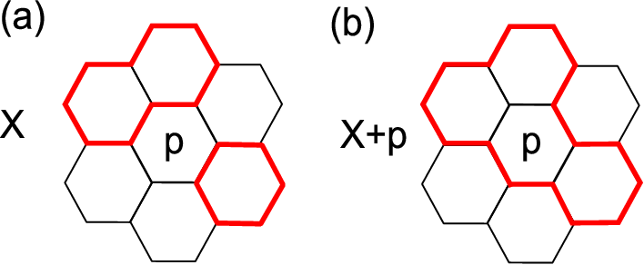
To derive the above identity (84), we first recall an analogous, but simpler identity involving 2D loop models. The 2D identity applies to 2D loop configurations that live on the links of a 2D planar trivalent lattice. It states that if we add a loop around the boundary of a single plaquette to form a new loop configuration , then
| (85) |
where and are the number of loops in the configurations and , and where is the number of occupied legs of the plaquette . (See Fig. 13 for an example). The 2D identity (85) is closely related to the 2D exactly soluble double semion model of Ref. 23, and can be established using the local rules that define that model.
To derive the 3D identity (84) from its 2D cousin (85), it is helpful to think about the configuration of green loops in , for a fixed red membrane configuration . These green loops lie on the surfaces of the red membranes . When we add a blue cube, this effectively adds a collection of green loops along all the red membranes that intersect the cube. Adding these green loops is similar to adding the loop in the 2D identity (85), so when we add these loops, the change in the parity of the number of green loops can be calculated by multiplying the factors on the right hand side of (85) over all the additional green loops. Taking the product of these factors gives the 3D identity (84).
Now that we have established the identity (84), we can complete our derivation of (80): substituting (84) into (83), we obtain
| (86) | |||||
where we made the change of variables in the second line. Finally, using the fact that and , we derive the required relation . The same argument works for .
All that remains is the third relation (81). In principle, one could establish (81) by writing out the explicit form of and calculating their commutators. However such a calculation would be tedious and not particularly illuminating. Therefore we use a different approach to show (81). We make use of two properties of the operators . The first property is the relation
| (87) |
which we just established above. The second property is that, for any closed membrane configuration ,
| (88) |
where is a phase factor that depends on . The latter property follows immediately from the definition of .
Using the above two properties (87) and (88), we will now show that the two operators commute with one another when acting on closed membrane states. The argument is simple. From property (88), we compute
| (89) | ||||
On the other hand, if we reverse the order we find
| (90) |
We need to show that the expressions on the right hand sides of (89) and (90) are equal. To this end, we note that property (87) implies that
| (91) |
Then, using property (88), we can write this as
| (92) |
so that
| (93) |
We now substitute (93) into equation (89). The result is
Likewise, if we substitute (93) into equation (90), we obtain the same expression:
implying that and commute when acting on closed membrane states.
Now that we know that and commute when acting on closed membrane states, we can immediately deduce that the combinations and commute when acting on arbitrary membrane states, since the operators and project onto states that are closed in the neighborhood of and . It then follows that the operators and commute with one another, since is a linear combination of and .
Appendix B Showing that the cylinder operators create braiding eigenstates
In this section we show that the blue cylinder operator creates loop excitations which are eigenstates of braiding measurements. Our argument consists of two parts. In the first part, we show that as long as obeys condition (46), then the loop excitations are guaranteed to be eigenstates of braiding measurements. In the second part, we check that does in fact obey (46). The second part can also be thought of as a derivation of Table 1 and Table 2, since we will see that the values in those tables are completely fixed by the requirement that obey equation (46).
B.1 Connection between equation (46) and braiding eigenstates
In this section we show that if obeys condition (46) then the blue cylinder operator is guaranteed to create loop excitations which are braiding eigenstates. We reprint equation (46) below for convenience:
| (94) |
Here and can be any two cylinders that share a common boundary while can be any membrane configuration whose intersection with the common boundary obeys the relevant cylinder operator boundary condition.
To begin, it is helpful to consider an example. Let be an excited state with a single red loop. We will call this red loop the “base loop.” Let be a blue cylinder operator that is linked with the base loop. Consider the state . This state contains two blue loops at the two ends of the cylinder , both of which are linked with the red base loop. Now, what we want to show is that these blue loops are eigenstates of braiding measurements. That is, we want to show that if we braid any other loop around one of these loops, the system returns to its original state multiplied by a complex number (in fact, a phase factor). We now translate this claim into a mathematical equation.
Consider, for example, braiding another blue loop around one of these loops. This braiding process can be implemented by applying a blue torus operator where the torus encircles the loop that we wish to braid around (see Fig. 12 for a similar geometry). The fact that the blue loop is an eigenstate of this braiding process is equivalent to the equation
| (95) |
Our task is to show that if obeys (94) then the operators obey equation (95). To establish this result, we first rewrite (95) in a more convenient form. We begin by recalling that since is a torus operator, it does not create any excitations — in other words, . Using this fact, the above equation can be written as
Next, multiplying both sides by gives
| (const.) |
Using the definition of , we rewrite the matrix elements on the left and right hand sides as:
Therefore, what we need to prove is
| (const.) |
or equivalently
| (96) |
We now prove (96). Focusing on the first ratio in (96), we note that the numerator and denominator can be represented graphically as
Here the thin vertical blue region corresponds to the intersection , while the gray areas on the left and on the right are meant to denote some arbitrary pictures corresponding to and . (We can assume without loss of generality that the pictures are of the above simple form, since we can use the path independence property, discussed below Eqs. (36), to deform and as we wish). Next we use equation (94) twice to break up the cylinder into three smaller cylinders, giving us
Taking the ratio of these expressions gives
In particular, we see that is independent of . In exactly the same way, one can show that is independent of . This proves equation (96): both terms on the left hand side are independent of , so their product must be independent of as well.
So far, we have shown that (94) implies the braiding eigenstate property in one case. The case we considered was a blue loop linked to a red base loop. We showed that the blue loop is a braiding eigenstate with respect to braiding another blue loop around it. To prove the general claim, we need to establish the same braiding eigenstate property for all other cases, that is all other combinations of red and blue loops. We will not discuss the other cases here, but it should be clear that the above argument is not specific to the case considered above and applies equally well to the other cases.
B.2 Checking that obeys equation (46)
In this section, we check that obeys equation (46) — or equivalently (94). To begin, we note that it suffices to check (94) for the case where the intersections and look like one of the four basic pictures shown in Table 1 and Table 2. The reason that we only need to consider this case is that the constraint equations (36) that define are local, so if (94) holds for basic pictures, then it automatically holds for general .
Let’s start with the simplest case: blue cylinder operators that create unlinked loops. In this case, the four basic pictures are those shown in Table 1. Specializing to these pictures, equation (94) reduces to different relations that we need to check. Many of these equations are redundant, so we only write the four independent ones below:
Next, we use the constraint equations (36) to reduce the pictures in the second and third lines to basic pictures:
Putting this together, we have
Letting
we can rewrite these equations as
| (97) |
Now let us compare with the values for given in Table 1:
| (98) |
where or . First, we can see that the above expressions (98) do in fact obey equations (97). Thus, we have successfully verified (94) for the case of an unlinked blue cylinder operator. In fact, we can see that (98) is actually the most general possible solution to the equations (97). Thus, the above calculation can also be regarded as a derivation of Table 1.
Next, we consider the case of a blue cylinder operator linked with a red base loop. We proceed in exactly the same way as in the unlinked case. First, we note that equation (94) reduces to different relations, of which are independent:
Next, we use the constraint equations (36) to derive:
Putting this together gives
Letting
we arrive at the following algebraic equations:
| (99) |
Let us compare with the values of given in the top panel of Table 2:
| (100) |
Again, we can see that the above expressions (100) obey (99). Thus, we have proven equation (94) for the case of a blue cylinder operator linked to a red base loop. We can also see that the above expressions are the most general solutions to these equations. Thus, our calculation can also be thought of as a derivation of the top panel of Table 2.
Finally, we consider the case of a blue cylinder operator linked with a blue base loop. Proceeding in the same away, we set
and we derive the algebraic equations
| (101) |
Again, it is easy to check that the values of given in the bottom panel of Table 2 obey equations (101). This establishes equation (94) for the case of a blue cylinder operator linked with a blue base loop.
References
- [1] M. Z. Hasan and C. L. Kane, Rev. Mod. Phys. 82, 3045 (2010).
- [2] X.-L. Qi and S.-C. Zhang, Rev. Mod. Phys. 83, 1057 (2011).
- [3] The 1D case is less interesting, since it is known that in the absence of symmetry all 1D bosonic systems belong to the same phase[29, 31, 32, 33, 30, 42] while all 1D fermionic systems belong to one of two phases.[30].
- [4] Here, when we say braiding statistics, we mean the complete set of algebraic data for anyon systems, including quantum dimensions and fusion rules. For more details, see e.g. Appendix E of Ref. \rev@citealpnumKitaevHoneycomb.
- [5] C. L. Kane and M. P. A. Fisher, Phys. Rev. B 55, 15832 (1997).
- [6] Here, we implicitly exclude 3D layered systems, like a stack of fractional quantum Hall states, from our discussion.
- [7] Y. Aharonov and D. Bohm, Phys. Rev. 115, 485 (1959).
- [8] M. G. Alford and F. Wilczek, Phys. Rev. Lett 62, 1071 (1989).
- [9] L. M. Krauss and F. Wilczek, Phys. Rev. Lett. 62, 1221 (1989).
- [10] J. Preskill and L. M. Krauss, Nucl. Phys. B 341, 50 (1990).
- [11] C. Aneziris, A. P. Balachandran, L. Kauffman, and A. M. Srivastava, Int. J. Mod. Phys. A 06, 2519 (1991).
- [12] M. G. Alford, K.-M. Lee, J. March-Russell, and J. Preskill, Nucl. Phys. B 384, 251 (1992).
- [13] J. C. Baez, D. K. Wise, and A. S. Crans, Adv. Theor. Math. Phys. 11, 707 (2007).
- [14] C. Wang and M. Levin, Phys. Rev. Lett. 113, 080403 (2014a).
- [15] S. Jiang, A. Mesaros, and Y. Ran, Phys. Rev. X 4, 031048 (2014).
- [16] J. Wang and X.-G. Wen, arXiv:1404.7854 (2014).
- [17] C.-M. Jian and X.-L. Qi, Phys. Rev. X 4, 041043 (2014).
- [18] C. Wang and M. Levin, arxiv:1412.1781 (2014b).
- [19] X. Chen, F. J. Burnell, A. Vishwanath, and L. Fidkowski, arxiv:1403.6491 (2015).
- [20] R. Dijkgraaf and E. Witten, Comm. Math. Phys. 129, 393 (1990).
- [21] A. Y. Kitaev, Annals of Physics 303, 2 (2003).
- [22] M. Levin and X.-G. Wen, Phys. Rev. B 67, 245316 (2003).
- [23] M. A. Levin and X.-G. Wen, Phys. Rev. B 71, 045110 (2005).
- [24] A. Hamma, P. Zanardi, and X.-G. Wen, Phys. Rev. B 72, 035307 (2005).
- [25] C. Castelnovo and C. Chamon, Phys. Rev. B 76, 184442 (2007).
- [26] J. B. Kogut, Rev. Mod. Phys. 51, 659 (1979).
- [27] X. Chen, Y.-M. Lu, and A. Vishwanath, Nature Communications 5, 3507 (2014).
- [28] Z.-C. Gu and X.-G. Wen, Phys. Rev. B 80, 155131 (2009).
- [29] F. Pollmann, A. M. Turner, E. Berg, and M. Oshikawa, Phys. Rev. B 81, 064439 (2010).
- [30] L. Fidkowski and A. Kitaev, Phys. Rev. B 81, 134509 (2010).
- [31] X. Chen, Z.-C. Gu, and X.-G. Wen, Phys. Rev. B 83, 035107 (2011a).
- [32] X. Chen, Z.-C. Gu, and X.-G. Wen, Phys. Rev. B 84, 235128 (2011b).
- [33] N. Schuch, D. Perez-Garcia, and I. Cirac, Phys. Rev. B 84, 165139 (2011).
- [34] X. Chen, Z.-C. Gu, Z.-X. Liu, and X.-G. Wen, Phys. Rev. B 87, 155114 (2013).
- [35] C.-H. Lin and M. Levin, in preparation. .
- [36] Y. Wan, J. Wang, and H. He, arxiv:1409.3216 (2014).
- [37] For example, toroidal operators can be decorated by string operators that encircle the torus while spherical membrane operators cannot be decorated in this way. See section III.3.4 for more details.
- [38] In fact, if our conjecture is correct then also belongs to the same phase as the Dijkgraaf-Witten models labeled by and , since the three Dijkgraaf-Witten models labeled by , and all belong to the same phase, when viewed as spin models rather than gauge theories.
- [39] J. Haah, Phys. Rev. A 83, 042330 (2011).
- [40] B. Zeng and X.-G. Wen, arxiv:1406.5090 (2014).
- [41] M. Levin and Z.-C. Gu, Phys. Rev. B 86, 115109 (2012).
- [42] F. Pollmann, E. Berg, A. M. Turner, and M. Oshikawa, Phys. Rev. B 85, 075125 (2012).
- [43] A. Kitaev, Ann. Phys. 321, 2 (2006).