Mercer kernels and integrated variance experimental design: connections between Gaussian process regression and polynomial approximation

Many elements of this work rely on the interpretation of the covariance kernel through its eigenfunctions, and to this end we recall the properties of a Mercer kernel. Let the kernel $K:\mathcal{X}\times\mathcal{X}\to\mathbb{R}$ be defined on a first-countable [16] space $\mathcal{X}\subseteq\mathbb{R}^{d}$ endowed with a strictly positive Borel measure $\mu$. Suppose that the kernel is continuous, positive semi-definite,

(3)

$$\quad\int_{\chi\times\chi}K(x,x^{\prime})g(x)g(x^{\prime})d\mu(x)d\mu(x^{\prime})\geq 0,\ \forall g\in L^{2}_{\mu}(\mathcal{X}),$$

and in $L^{1}(\mathcal{X},\mu)$

(4)

$$\int_{\chi}\left|K(x,x)\right|d\mu(x)<\infty.$$

Additionally we define the integral operator $T_{K}:L^{2}_{\mu}(\mathcal{X})\to L^{2}_{\mu}(\mathcal{X})$ such that $T_{K}f=\int_{\chi}K(x,x^{\prime})f(x^{\prime})d\mu(x^{\prime}).$ This operator has a countable system of eigenvalues $\lambda_{j}$ that are non-negative and that satisfy

$$\sum_{j=1}^{\infty}\lambda_{j}^{2}<\infty.$$

The eigenfunctions $\phi_{i}$ of $T_{K}$ form an orthonormal basis of $L^{2}_{\mu}(\mathcal{X})$. These eigenfunctions and eigenvalues can be used to define the reproducing kernel Hilbert space (RKHS) associated with the kernel [49]. Mercer’s theorem lets us represent $K$ as a convergent series in terms of this eigensystem.

When comparing GP regression with pseudospectral approximation in later sections of this paper, we will also use the notion of a truncated kernel. These are kernels for which $\lambda_{i>\ell}=0$, and for which we can equivalently write (5) as

$$K(x,x^{\prime})=\sum_{i=1}^{\ell}\lambda_{i}\phi_{i}(x)\phi_{i}(x^{\prime}).$$

One common example of a truncated kernel is a polynomial kernel, e.g., $K(x,x^{\prime})=(x^{T}x^{\prime}+1)^{p}$, where $p$ is a positive integer.

We can use Mercer’s theorem to write the integrated posterior variance of the Gaussian process in terms of the eigensystem $(\lambda_{i},\phi_{i})$. The posterior variance at any point in the domain is $c(x):=C(x,x)$. The integrated variance then becomes

	$\displaystyle\int c(x)d\mu(x)$	$\displaystyle=\int\left(K(x,x)-K(\bm{x},x)^{T}\mathbf{R}\,K(\bm{x},x)\right)d\mu(x)$
		$\displaystyle=\int K(x,x)d\mu(x)-\int\sum_{i=1}^{\infty}\sum_{j=1}^{\infty}\lambda_{i}\lambda_{j}\bm{\phi}_{i}^{T}\mathbf{R}\bm{\phi}_{j}\phi_{i}(x)\phi_{j}(x)d\mu(x)$
(6)			$\displaystyle=\sum_{i=1}^{\infty}\lambda_{i}-\sum_{i=1}^{\infty}\lambda_{i}^{2}\bm{\phi}_{i}^{T}\mathbf{R}\bm{\phi}_{i},$

where $\bm{\phi}_{i}:=\left[\phi_{i}(x_{1}),\ldots,\phi_{i}(x_{N})\right]^{T}.$ The first term is the integrated variance of the prior. The second term, which is always non-negative, reflects reduction in the integrated prior variance due to conditioning on the data. We will now examine how experimental design procedures can use this integrated variance as an optimization objective.

For a chosen number of experiments $N\geq 1$ and a fixed prior covariance kernel $K$, our optimal experimental design is a set of evaluation points $\bm{x}^{\ast}:=\left[x_{1}^{\ast},\ldots x_{N}^{\ast}\right]$, $x_{i}^{\ast}\in\mathbb{R}^{d}$, minimizing the integrated posterior variance:

(9)

$$\bm{x}^{*}=\arg\min_{\bm{x}\in\mathcal{U}}\int_{\mathcal{X}}c(x|\bm{x})d\mu(x).$$

Here $\mathcal{U}$ is the space of all feasible experiments and the posterior variance is specified via (2).

While this objective function is similar to that in [58], here we will employ a continuous space $\mathcal{U}$ of possible experiments. Also, we will solve the optimization problem (9) both in a non-greedy fashion (finding all $N$ design points simultaneously) and using greedy updates with varying batch sizes. In this section the number of design points $N$ and the prior covariance kernel $K$ will be considered fixed. Later, in Section 5.4, we will consider closed-loop design procedures that alternate between batch minimization of IVAR and updates of the covariance kernel.

Statistical criteria underlie many other experimental design procedures for Gaussian process regression [53]. Two popular techniques include minimizing the conditional entropy of the Gaussian process at unobserved locations, or maximizing the mutual information (MI) between the locations at which experiments are performed and the rest of the design space. Our numerical results will compare IVAR designs with MI and entropy-based designs because the latter have algorithms specifically tailored for Gaussian process regression. For a comparison between these two methods and additional design procedures, e.g., based on classical alphabetic optimality criteria, we refer to [34].

The conditional entropy design procedure seeks experiments that reduce the uncertainty, as measured by entropy $H$, across a typically finite set of possible simulation locations. If the set of candidate experimental locations is denoted by $\mathcal{D}$ and $\bm{x}\subset\mathcal{D}$ are the chosen locations, then $x^{c}:=\mathcal{D}\setminus\bm{x}$ are the locations at which the entropy is evaluated. In particular, one seeks $\bm{x}$ to minimize the conditional entropy $H(F_{\bm{x}^{c}}|F_{\bm{x}})=-\int p(f_{\bm{x}^{c}},f_{\bm{x}})\log p(f_{\bm{x}^{c}}|f_{\bm{x}})df_{\bm{x}^{c}}df_{\bm{x}}$, where $F_{\bm{s}}$ is a random variable representing the outputs of the simulation model at a set of inputs $\bm{s}$ and $p$ denotes a probability density. Minimizing this function is shown to be NP-hard in [33]. In practice, one instead employs greedy but suboptimal algorithms that add one experiment at a time—for example, adding each experiment at the location where the conditional entropy is largest [60, 9, 38]. In the context of GPR, $F_{\bm{x}}$ and $F_{\bm{x}^{c}}$ are jointly Gaussian; this procedure then becomes equivalent to greedily adding experiments at the locations of highest variance, and is commonly called the MacKay criterion (ALM). Other algorithms for choosing a subset of points to minimize the conditional entropy are based on the DETMAX algorithm [41], demonstrated for GP regression in [10]

The mutual information criterion for experimental design considers the change in the entropy of $F_{\bm{x}^{c}}$ before and after performing experiments at locations $\bm{x}$: $H(F_{\bm{x}^{c}})-H(F_{\bm{x}^{c}}|F_{\bm{x}})$, which is equivalent to the mutual information of $F_{\bm{x}}$ and $F_{\bm{x}^{c}}$. This objective is also typically maximized in a greedy fashion: from the candidate set of experiments $\mathcal{D}$, the element which yields the greatest MI is chosen at each iteration. Unlike the conditional entropy, however, MI is submodular, guaranteeing that a greedy approach performs within a constant factor of the full $N$-experiment maximization [34]. The greedy procedure requires the inversion of a matrix containing the covariance between every pair of candidate experiments, which arises when computing the entropy on the set of all simulation locations. If one is choosing $N$ experiments from a set of $M\gg N$ candidates, each iteration then requires inverting a matrix of size $M\times M$. This expense is typically large and many recent efforts have aimed at reducing it. [34] reduces the cost of each iteration to $\mathcal{O}(M)$ by using specialized local kernels. [3] points out that the quality of an MI design depends crucially on the candidate set, and modifies the greedy algorithm of [34] to be more robust by resampling the set of candidate experiments after each new point is chosen.

Besides the choice of objective, our IVAR-based design algorithm differs from the entropy and MI approaches above in other fundamental ways. First, we select experiments from a continuous design space and thus avoid the challenges of combinatorial optimization. In this sense, we follow the approach of [52] by solving a continuous optimization problem using gradient descent algorithms. Second, as described in Section 3.1.2, our approach can identify multiple experiments simultaneously. Designing batch experiments is advantageous because interactions between the experiments are taken into account; we will demonstrate this advantage empirically in the next section. Our continuous design approach also takes several steps beyond [52]. First, we do not employ particular patterns or partitions to simplify the design space. And as described earlier, we introduce a sample-average approximation of the IVAR objective. This helps design experiments on complex input domain geometries by penalizing proximity to the domain boundaries; the objective automatically becomes large in locations where there are few samples. We will also address the “pileup” problem identified in [52], explaining it in terms of the design size relative to correlation kernel complexity.

In some sense, if evaluating $f$ is sufficiently expensive, then the computational cost of finding a good design is immaterial. But the design procedures described above can have very different costs, and in practice one may not want the computational effort required for experimental design to be too large. Table 1 summarizes the computational complexity of evaluating and optimizing the various experimental design objectives considered above. In the IVAR scenarios, $N_{mc}$ denotes the number of Monte Carlo points sufficient for (10), where typically $N_{mc}\gg N$. For the entropy and MI criteria we assume that the number of candidate designs $N_{E}=|\mathcal{D}|\gg N$. Finally, we assume that optimizing the IVAR objective requires $L$ objective and/or gradient evaluations, where typically $L\ll N_{mc}$.

Greedy minimization of the conditional entropy (ALM) requires $N$ iterations. In each iteration the variance must be computed at $N_{E}$ locations.²² 2 Although we have described a discrete approach for ALM minimization, a continuous optimization approach is also possible. But the pointwise variance of a GP has many local maxima, and a multi-start procedure would likely be necessary for continuous optimization to be competitive with discrete enumeration. It is then unclear whether continuous optimization would in fact be more efficient in this case. At iteration $k<N$, this variance computation requires an $\mathcal{O}(k^{3})$ inversion followed by $N_{E}$ variance evaluations, each of complexity $\mathcal{O}\left(k^{2}\right)$. Thus the complexity for step $k$ is $\mathcal{O}(k^{3}+N_{E}k^{2})$. The total complexity is thus $\mathcal{O}\left(\sum_{k=1}^{N}k^{3}+N_{E}k^{2}\right)=\mathcal{O}\left(N^{4}+N_{E}N^{3}\right)$.

The ALM approach is often the computationally cheapest option, but not if $N_{E}>LN_{mc}/N$. If $N_{E}$ and $N_{mc}$ are of comparable magnitude, then the comparison of entropy and IVAR minimization depends on whether $L/N<1$, i.e., how the number of optimization iterations (in the continuous case) compares to the number of candidate design points (in the discrete case). We also see that the MI design becomes very expensive for large $N_{E}$; a small candidate design set must be chosen for the MI procedure to remain tractable. Using a smaller candidate set, however, increases the possibility that the chosen designs will perform poorly.

As discussed above, GP regression with $\sigma^{2}=0$ (and a kernel rank $\ell>N$) corresponds to interpolation. In this setting, it is useful to analyze the quality of interpolation on IVAR design points. The Lebesgue constant is often used to bound the error of a polynomial interpolant relative to the best approximation in a polynomial space of equivalent degree, but it can also be used to analyze interpolation with positive definite kernels, corresponding here to the posterior mean of the GP. Let $m(x)$ denote the interpolant or posterior mean, and let $m^{\ast}(x)$ denote the best approximation of $f$, in the $L_{\infty}$ sense, from the finite-dimensional kernel space $H(K,\bm{x}_{N})=\Span\{K(\cdot,x_{1}),\ldots,K(\cdot,x_{N})\}$. We restrict our attention to approximation on compact domains $\mathcal{X}\subseteq\mathbb{R}^{d}$. Then the $L^{\infty}$ interpolation error is bounded as [17]

$$\|f-m\|_{L_{\infty}(\mathcal{X})}\leq(1+\Lambda_{K,\bm{x}_{N}})\|f-m^{\ast}\|_{L_{\infty}(\mathcal{X})},$$

and moreover we have [13],

$$\|m\|_{L_{\infty}(\mathcal{X})}\leq\Lambda_{K,\bm{x}_{N}}\|\bm{y}\|_{\ell_{\infty}}.$$

The Lebesgue constant $\Lambda_{K,\bm{x}_{N}}$ for prior kernel $K$ and design points $\bm{x}_{N}$ is

(11)

$$\Lambda_{K,\bm{x}_{N}}=\max_{x\in\mathcal{X}}\sum_{j=1}^{N}|u_{j}(x)|,$$

where $\{u_{j}(x)\}_{j=1}^{N}$ are the cardinal functions satisfying $u_{j}(x_{i})=\delta_{ij}$, such that the interpolant can be written as $m(x)=\sum_{j=1}^{N}y_{j}u_{j}(x)$ with $y_{j}=f(x_{j})$. We evaluate the cardinal functions as in [17] by solving the linear system

(12)

$$\mathbf{R}^{-1}\bm{u}(x)=K(\bm{x},x),$$

where $\bm{u}(x)=[u_{1}(x)\ldots u_{N}(x)]$.

Now we conduct a simple numerical experiment to evaluate the Lebesgue constants of point sets arising from IVAR minimization. We find IVAR designs on the domain $\mathcal{X}=[-1,1]$ with squared exponential kernel $K(x,x^{\prime})=\exp({-(x-x^{\prime})^{2}/2l^{2}})$. Figure 1 shows the associated Lebesgue constants as a function of number of design points $N$, for various correlation lengths $l$. Several interesting trends are observed. First, we see that for any value of $l$, the Lebesgue constant is exactly one for sufficiently small $N$. This observation is consistent with the asymptotic estimate for $l\rightarrow 0$ in [50]. The Lebesgue constant reverts to one for small point sets because the IVAR criterion ensures that the points are well separated, and hence the cardinal functions do not overlap. Once a certain threshold value of $N$ is attained, however, the Lebesgue constant begins to increase; this threshold value is smaller for larger values of the correlation length $l$. This transition coincides with interactions among the cardinal functions: Figure 2 shows cardinal functions for $N=16$ and $l=0.1$, just beyond the threshold where interaction becomes significant. In this regime, the Lebesgue constant increases steadily with $N$. For a sufficiently large $N$, $\mathbf{R}^{-1}$ becomes poorly conditioned and direct computations of the interpolant, the cardinal functions, and the Lebesgue constant are no longer numerically stable. From the Bayesian perspective, this ill-conditioning corresponds to the “complexity” of the RKHS associated with the prior kernel—i.e., the effective number of nonzero eigenvalues in (5)—being exceeded by the data.

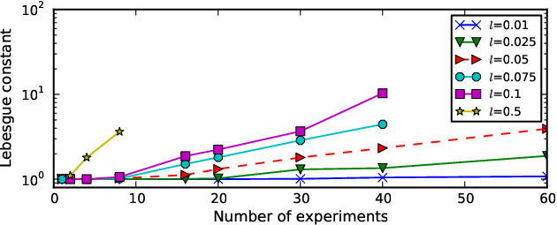
The success of the IVAR optimization procedure itself also depends on how $N$ relates to the complexity of the kernel. In the small-$N$ and small-$l$ regime (intuitively, “too few” points relative to the complexity of the kernel), the IVAR cost function is relatively flat as a function of the design coordinates $\bm{x}$, and distinguishing the quality of different designs becomes difficult. By contrast, in the large-$N$ and large-$l$ regime (“too many” points relative to the complexity of the kernel), the IVAR value itself is exceedingly small and the problem is poorly conditioned, as described above. Away from these limiting regimes, however, the IVAR design procedure yields relatively slow growth in the Lebesgue constant and thus relatively stable interpolation.

Here we illustrate IVAR designs on variety of input domains $\mathcal{X}$, and compare the performance of IVAR designs with that of designs obtained through conditional entropy minimization or MI maximization. We highlight designs and approximations on irregular input domains (e.g., domains that are neither hypercubes nor $\mathbb{R}^{d}$), which are critical in many real-world applications. In particular, irregular domains often arise as a result of domain partitioning by a discontinuity detection algorithm, for models whose outputs are piecewise smooth. For example, in [29, 26] the authors automatically partition the input domain of a genetic toggle switch model that exhibits a phase transition. Following this partitioning, function approximation proceeds on two separate but irregular domains. In [55, 56] the authors study a climate model which exhibits a discontinuity. Discontinuity detection is used to split the input domain into two irregular subdomains, and is followed by function approximation. We will thus attempt to show the applicability of our algorithm to input domains that are characteristic of such problems, which have no guarantees of convexity or even connectedness.

In most of our numerical experiments, we employ an isotropic squared exponential kernel $K(x,y)=\exp(-\|x-y\|^{2}/2l^{2})$ and we set $\sigma^{2}=10^{-10}$; the only exception is in Section 4.2.2, which uses a periodic kernel to contrast space-filling designs with designs that are adapted to the kernel. Entropy minimization is pursued through the ALM approach described earlier; each experiment is chosen by comparing the variance at $N_{E}=10^{4}$ possible experimental locations sampled according to the parameter measure $\mu$ on $\mathcal{X}$. For MI maximization, we select designs from $N_{E}=200$ candidate locations generated by the space-filling LJ design. The size of the MI candidate set is chosen so that the computational times of the different experimental design procedures are comparable; it is also comparable to sizes used in the literature [3]. We find that small changes in the size of this candidate set do not qualitatively change the results reported below.

Finally, we define the relative $L^{2}$ error of a GP approximation as $\|f-m\|_{L^{2}_{\mu}}/\|f\|_{L^{2}_{\mu}}$, and we estimate it using $10^{5}$ Monte Carlo samples. While in the previous section we considered $L^{\infty}(\mathcal{X})$ error, recall that the IVAR objective function reflects the expectation of a squared $\mu$-averaged error. Thus $L^{2}_{\mu}$ is a logical metric of quality. Other efforts, e.g., [37], empirically evaluate the $L^{2}$ and $L^{\infty}$ errors of approximations resulting from a variety of other design criteria.

In this section, we recall the basics of pseudospectral approximation. Consider a set of basis functions $\{\psi_{i}(x)\}$ comprising a complete orthonormal system in $L^{2}_{\mu}$. Pseudospectral approximation takes advantage of orthonormality

$$\left<\psi_{i},\psi_{j}\right>_{\mu}=\int\psi_{i}(x)\psi_{j}(x)d\mu(x)=\delta_{ij},$$

to compute the projection of a function $f$ onto a subspace of $L^{2}_{\mu}$ spanned by $\ell$ basis functions. The orthogonal projection

$$f_{\ell}(x)=\sum_{i=1}^{\ell}\left<f,\psi_{i}\right>_{\mu}\psi_{i}(x).$$

converges in the $L^{2}_{\mu}$ sense as the subspace grows: $\lim_{\ell\to\infty}\int\left(f_{\ell}-f\right)^{2}d\mu=0$. Pseudospectral approximation departs from exact orthogonal projection by using numerical quadrature to approximate the inner products $\left<f,\psi_{i}\right>$. In particular, one seeks an orthogonalizing set of nodes and weights, $\mathcal{Q}=\left\{(x_{k},w_{k}):k=1\ldots N\right\}$, i.e., a quadrature rule that computes the inner products between the first $\ell$ basis functions exactly:

(13)

$$\left<\psi_{i},\psi_{j}\right>_{\mu}=\sum_{k=1}^{N}w_{k}\psi_{i}(x_{k})\psi_{j}(x_{k}),\ i,j=1,\ldots,\ell.$$

This choice eliminates internal aliasing error [7], though the pseudospectral approximation will still exhibit external aliasing error, since $f$ is not necessarily in the span of $\{\psi_{1},\ldots,\psi_{\ell}\}$. Given an orthogonalizing rule (13), a pseudospectral approximation $\hat{f}_{\ell}$ can be written as

(14)

$$\hat{f}_{\ell}(x)=\sum_{i=1}^{\ell}\left(\sum_{k=1}^{N}w_{k}f(x_{k})\psi_{i}(x_{k})\right)\psi_{i}(x)=\sum_{k=1}^{N}\left[w_{k}f(x_{k})\left(\sum_{i=1}^{\ell}\psi_{i}(x_{k})\psi_{i}(x)\right)\right].$$

In subsequent analysis, it will be convenient to express $\hat{f}_{\ell}(x)$ in matrix notation. Let $\mathbf{W}:=\mathop{\operator@font diag}\nolimits(w_{1},\ldots w_{N})$, $\bm{y}:=\left[f(x_{1}),\ldots,f(x_{N})\right]$ and $\bm{\psi}_{i}:=\left[\psi_{i}(x_{1}),\ldots,\psi_{i}(x_{N})\right]$. Then

(15)

$$\hat{f}_{\ell}(x)=\bm{y}^{T}\mathbf{W}\sum_{i=1}^{\ell}\bm{\psi}_{i}\psi_{i}(x).$$

Examples of $\{\psi_{i}\}$ and $\mathcal{Q}$ include one-dimensional orthogonal polynomial families and their corresponding Gaussian quadratures; or tensorized versions of each in multiple dimensions. However, the basis functions $\psi_{i}$ do not in general need to be polynomials, and other quadrature rules besides Gaussian rules may exist. Using Mercer’s theorem, we can already see that $\sum_{i=1}^{\ell}\psi_{i}(x)\psi_{i}(y)$ can be interpreted as a truncated kernel $K^{\ell}(x,y)$ with eigenvalues that do not decay, and we can interpret the pseudospectral approximation given in (15) as a weighted combination of such kernels.

To begin our comparison, we will fix two of the choices involved in surrogate modeling and evaluate the impact of the third. In particular, this section will compare the impact of different algorithms—i.e., using pseudospectral approximation versus GP regression—for identical experiments and for the same or similar approximation spaces. Because pseudospectral approximation requires experiments to be chosen according to an orthogonalizing rule, we will also use these experiments for GP regression. We are now left to relate the basis for the pseudospectral approximation to the GP kernel, as these objects determine the approximation space.

Theorem 1 lets us represent any Mercer kernel, and the corresponding GP posterior mean function, using the eigenfunctions. With this connection, we first develop a more general result than required. Specifically, we show that when the basis for pseudospectral approximation comprises a subset of the eigenfunctions of a given kernel, then the $L^{2}_{\mu}$-norm of the difference between the resulting GP posterior mean function and the pseudospectral approximation may be bounded. Results for identical approximation spaces follow immediately as a corollary of this general case.

For the result below, we will assume that we have a Mercer kernel consisting of $\ell_{GP}$ eigenfunctions, where $\ell_{GP}$ could be finite or infinite, and a spectral expansion consisting of the first $\ell\leq\ell_{GP}$ eigenfunctions, where $\ell$ is finite. The approximations will be constructed from $N$ evaluations of the function $f$, performed at nodes of a quadrature rule $\left\{(x_{i},w_{i})\right\},i=1\ldots N$, that orthogonalizes the first $\ell$ eigenfunctions. Clearly $N$ depends on $\ell$. Let $\mathbf{USU}^{T}$ be the eigendecomposition of the matrix of covariances $K(x_{i},x_{j})$ among all the design points computed without a nugget, i.e., $\mathbf{R}^{-1}-\sigma^{2}\mathbf{I}=\mathbf{USU}^{T}$. $\mathbf{S}$ is a diagonal matrix with elements $\mathbf{S}=\mathop{\operator@font diag}\nolimits(s_{1},\ldots,s_{N})$. Finally, assume a zero mean prior $m_{0}(x)=0$ for the GP model. The latter assumption does not restrict the generality of our results. In fact, one can transform the problem from one of approximating $f$ to one of approximating $g=f-m_{0}$, for some fixed function $m_{0}(x)$. Of course, this transformation requires one to translate the data $\bm{y}$ accordingly. Under these conditions, we have the following result, whose proof is given in Appendix A.

We can consider a relative notion of error by dividing each side by $\|\bm{y}\|_{2}^{2}$. Furthermore, since we are dealing with bounded functions $f$ and finite amounts of data, we can always normalize and center the data to make $\|\bm{y}\|_{2}=\mathcal{O}(1)$. The difference between the two approximations described in Theorem 2 has two sources. First is the contribution of kernel eigenfunctions that are not in the pseudospectral approximation basis, i.e., the summations involving $j>\ell$ above. Second is the contribution of the noise term $\sigma^{2}$.

Because the kernel eigenfunctions span the RKHS containing the GP posterior mean, the case of equivalent approximation spaces for pseudospectral approximation and GP regression follows simply by setting $\ell_{GP}=\ell<\infty$. This case is highlighted by Corollary 3.

In this case, the difference between approximations is due only to the nugget $\sigma^{2}>0$ and the smallest eigenvalue of the covariance matrix as indicated by $s_{N}$. If we additionally have that $N\leq\ell_{GP}$, then the design covariance matrix $\mathbf{R}^{-1}$ remains invertible (i.e., with $s_{N}>0$) even as $\sigma^{2}\to 0$, yielding zero difference between the approximations. This occurs, for example, in the case of kernels constructed from fully tensorized polynomial eigenfunctions and tensorized Gaussian quadrature rules, where $N=\ell=\ell_{GP}$.

We also note that the bound in Theorem 2 depends on the minimum eigenvalue of the covariance matrix, represented (after diagonalization) by $\mathbf{S}+\sigma^{2}\mathbf{I}$. If $\mathbf{S}$ is nearly rank-deficient and the nugget is sufficiently small, then the bound can be large. This situation is not purely an artifact of the theory; indeed, it corresponds to a poorly conditioned numerical problem, where the actual difference between the two approximations may be large as well. One may imagine a case where $\mathbf{R}$ is not invertible, e.g., too many quadrature nodes are used and the GP kernel is finite rank; in this case the computation of $m$ becomes unstable whereas the computation of $\hat{f}_{\ell}$ can still proceed in a stable manner.

Besides bounding the difference between approximations, we can also analyze the impact of an orthogonalizing experimental design on the integrated variance of the GP posterior. Consider, again, a kernel consisting of $\ell_{GP}$ eigenfunctions and a training set corresponding to the nodes of a quadrature rule $\mathcal{Q}$ that orthogonalizes the first $\ell$ eigenfunctions. We begin by splitting (6) into summations involving the first $\ell$ eigenfunctions and the remaining $\ell+1$ to $\ell_{GP}$ eigenfunctions:

$\displaystyle\int c(x)d\mu(x)$

$\displaystyle=\sum_{i=1}^{\ell}\lambda_{i}\left(1-\lambda_{i}\bm{\phi}_{i}^{T}\mathbf{R}\bm{\phi}_{i}\right)+\sum_{i=\ell+1}^{\ell_{GP}}\lambda_{i}\left(1-\lambda_{i}\bm{\phi}_{i}^{T}\mathbf{R}\bm{\phi}_{i}\right).$

The second term in this expansion represents the contribution of the extra eigenfunctions to the integrated variance. We cannot comment on how our training points will affect this term because they are designed to have special properties only for the first $\ell$ eigenfunctions. But we can use these properties to analyze the first term above, thus describing the impact of an orthogonalizing rule on the associated integrated variance. Note that the weights $\mathbf{W}$ do not explicitly enter the GP regression; nonetheless, as we show in Appendix B, this portion of the integrated variance can be rewritten as:

(17)

$\displaystyle\sum_{i=1}^{\ell}\lambda_{i}\left(1-\lambda_{i}\bm{\phi}_{i}^{T}\mathbf{R}\bm{\phi}_{i}\right)$

$\displaystyle=\sum_{i=1}^{\ell}\lambda_{i}\bm{\phi}_{i}^{T}\mathbf{W}\left(\sum_{j=\ell+1}^{\ell_{GP}}\lambda_{j}\bm{\phi}_{j}\bm{\phi}_{j}^{T}+\sigma^{2}\mathbf{I}\right)\mathbf{R}\bm{\phi}_{i}.$

This expression consists of interactions between the first $\ell$ eigenfunctions and the last eigenfunctions; it also includes the impact of the nugget. The eigenfunction interactions are expected because the design only orthogonalizes the first $\ell$ eigenfunctions; errors are incurred when the numerical inner product is taken between one of the first $\ell$ eigenfunctions and one of the remaining eigenfunctions. We see that if $\ell=\ell_{GP}$, the integrated variance is of the order of the noise $\sigma^{2}$ as expected. When additionally $\sigma^{2}=0$, the integrated variance is zero. An orthogonalizing design ensures that the integrated variance captures only the contributions of eigenfunctions which are not orthogonalized.

The preceding results highlight some of the assumptions underlying the practical application of these two surrogate construction methodologies. When using a pseudospectral approximation, one implicitly assumes that the true function’s projection onto basis functions not included in the expansion (and hence not orthogonalized by the underlying design) is small. Otherwise, more points and basis functions should be added to the approximation; indeed, adaptive basis selection is the concern of a vast array of approximation methods, pseudospectral and otherwise. In GP regression, a properly chosen kernel is one whose eigenvalue decay matches the decay of the spectral coefficients of the true function. In this case the function will lie in the RKHS associated with the kernel and an accurate approximation can readily be achieved. These two approaches interact through the integrated variance. The orthogonalizing rule in a pseudospectral approximation ensures that the difference between $f$ and $f_{\ell}$ lies mostly in the span of the eigenfunctions $\phi_{k>\ell}$. Correspondingly, this rule forces the IVAR, a measure of the uncertainty and error (via the Bayes risk) of the GP approximation, to retain contributions only from the same subspace (that spanned by $\{\phi_{k>\ell}\}$). We also see that the difference between the GP posterior mean and pseudospectral approximation is dominated by these extra eigenfunctions.

It is instructive to consider the tradeoff between exactly orthogonalizing fewer basis functions or, for the same design points, generating an approximation using more basis functions than can be orthogonalized. The latter corresponds to performing GP regression under the conditions of Theorem 2 with $\ell_{GP}>\ell$.

Consider the function $f(x)=\sin(\pi x+0.2)$ for $x\in\mathbb{R}$ with standard Gaussian weight $\mu$. We will use a Gauss-Hermite quadrature rule with $N=20$ points to construct a pseudospectral approximation of $f$ with the first $\ell=20$ Hermite polynomials (degrees 0 to 19) as basis functions. We compare this approximation to Gaussian process regression on the same points using the Mehler kernel [57]

(18)

$$K(x,y;t)=\frac{1}{\sqrt{1-t^{2}}}\exp\left(-\frac{1}{2}\frac{\left(x\right)^{2}t^{2}-2txy+\left(y\right)^{2}t^{2}}{1-t^{2}}\right),$$

which is a closed-form expression for $K(x,y)=\sum_{i=0}^{\infty}t^{i}\phi_{i}(x)\phi_{i}(y)$, where $\{\phi_{i}\}$ are again normalized Hermite polynomials. The nugget $\sigma^{2}=0$ and the decay constant $t=0.8$. In this way we compare two surrogates using identical experiments and closely related approximation spaces: the approximation space of the former is contained in that of the latter. But the two surrogates use different approaches for combining the same function evaluations into an approximation. GP regression approximates $f$ using an infinite collection of polynomial eigenfunctions, with more emphasis on those associated with higher eigenvalues, while pseudospectral approximation projects $f$ onto finite polynomial basis, with the exactness of the projection limited by external aliasing.

Figure 9 shows the results of this experiment. First, we note that the relative $L^{2}_{\mu}$ errors are $8.7\times 10^{-3}$ for pseudospectral approximation and $1.8\times 10^{-3}$ for the GP mean function. Perhaps more interesting than this improvement, however, is the spectrum of the error associated with each approximation. The left panel of Figure 9 shows the projections of the errors $e_{ps}(x)=\hat{f}_{\ell}(x)-f(x)$ and $e_{gp}(x)=m(x)-f(x)$ onto each basis function $\phi_{i}$, i.e., $|\langle e,\phi_{i}\rangle|$. For reference, the right panel shows how much energy $f$ has in each basis direction, via the magnitudes of the exact projections $|\langle f,\phi_{i}\rangle|$. (All projections are computed with extremely high-order quadrature.) We see that the projection of the pseudospectral approximation error $e_{ps}$ onto the first few basis functions is small, even though $f$ itself has significant energy in these directions. The projection of $e_{ps}$ then rises with the basis index and peaks around an index of 20; it then begins to decay, just as the exact coefficients $\langle f,\phi_{i}\rangle$ themselves decay in magnitude. The projection of the GP error, on the other hand, is flatter across the indices. It rises slightly for the first few basis functions and then begins to decay somewhat more slowly. The basis functions for which the orange line (GP error) lies below the red line (PSA error) correspond to relatively large coefficient values; this results in a lower $L^{2}$ error overall.

As a preview of the next section, we include a third line in Figure 9 representing GP regression performed with a 20-point IVAR-minimizing design. The relative $L^{2}_{\mu}$ error of this approximation is even smaller: $1.0\times 10^{-5}$. And the spectrum of its error, shown with the grey line in the left panel, is even flatter than that of the quadrature-based GP approximation. This result amplifies the previous trend: compared to pseudospectral approximation, GP regression spreads its error more evenly over the spectrum. Departing from an orthogonalizing design allows this error to be spread even more broadly.

Our next goal is to compare GP regression and pseudospectral approximation when the approximation spaces are similar, but the experimental designs (and the algorithms) differ. We have already seen that RKHS containing the GP mean can coincide with the range of the pseudospectral approximation operator in the case of a finite-rank GP kernel: the eigenfunctions of the kernel can simply be used as the basis for the pseudospectral approximation. In the numerical comparisons below, however, we would like to allow the GP kernel to have infinite rank. This choice is more representative of how GP regression is used in practice, and in principle may allow the GP mean to better approximate a wider variety of functions. Of course, the eigenvalues of the kernel need to decay, so that we have a bounded kernel.

We will therefore use the Mehler kernel (18) as in Section 5.3, and consider target functions whose inputs are endowed with standard Gaussian weight on $\mathbb{R}^{d}$. The eigenfunctions of the Mehler kernel are Hermite polynomials, which we use as basis functions for pseudospectral approximation. In $d>1$ dimensions, we use a tensorized version of the Mehler kernel: $K(x,y;t_{1},\ldots,t_{d})=\prod_{i=1}^{d}K(x^{(i)},y^{(i)};t_{i})$, where $t_{i}$ now governs the decay rate of the eigenvalues associated with the univariate eigenfunctions in dimension $i$.

To design experiments for GP regression, we use IVAR minimization in combination with adaptation of the covariance kernel hyperparameters (e.g., correlation lengths) and the nugget $\sigma^{2}$. In particular, we choose these parameters by maximizing the log-marginal likelihood,

(19)

$$\log p(\bm{\hat{y}}|\bm{x},\theta)=-\frac{1}{2}\bm{\hat{y}}^{T}\mathbf{R}\bm{\hat{y}}-\frac{1}{2}\log|\mathbf{R}^{-1}|-\frac{N}{2}\log 2\pi,$$

with respect to the complete set of hyperparameters (including $\sigma^{2}$), denoted by $\theta$. Our approach interleaves kernel adaptation with batch IVAR design. The batch size for each design is described in each example, but the number of Monte Carlo points used to evaluate the IVAR objective is fixed at $N_{mc}=10^{4}$.

For pseudospectral approximation, we use a state-of-the-art adaptive Smolyak algorithm [7], which adaptively enriches both the approximation basis and the experimental design using a greedy heuristic. The approximation is essentially a Smolyak sum of full tensor-product polynomial approximations, each computed using a pseudospectral approach. We use this approach because a regular tensor-product approach becomes infeasible for more than a few dimensions; hence many sparse grid [2] and dimension-adaptive [24] polynomial approximation algorithms have been developed. The Smolyak algorithm in [7] uses generalized sparse grids and dimension adaptivity and thus provides a useful benchmark for comparison with kernel-adaptive GP. It is implemented in the MIT Uncertainty Quantification framework (MUQ) [47]. Since the input domain is endowed with Gaussian measure, the sparse grid design is based on one-dimensional Gauss-Hermite quadrature rules, with the number of points growing exponentially with the level of the sparse grid.

References

- [1] A. C. Atkinson, A. N. Donev, and R. D. Tobias. Optimum experimental designs, with SAS, volume 34. Oxford University Press Oxford, 2007.
- [2] V. Barthelmann, E. Novak, and K. Ritter. High dimensional polynomial interpolation on sparse grids. Advances in Computational Mathematics, 12(4):273–288, 2000.
- [3] J. Beck and S. Guillas. Sequential design with mutual information for computer experiments (MICE): Emulation of a tsunami model. arXiv preprint arXiv:1410.0215, 2014.
- [4] J. Buescu. Positive integral operators in unbounded domains. Journal of Mathematical Analysis and Applications, 296(1):244–255, 2004.
- [5] E. B. Christoffel. Über die gaußische quadratur und eine verallgemeinerung derselben. Journal für die reine und angewandte Mathematik, 55:61–82, 1858.
- [6] D. A. Cohn. Neural network exploration using optimal experiment design. Neural networks: the official journal of the International Neural Network Society, 9(6):1071–1083, August 1996.
- [7] P. R. Conrad and Y. M. Marzouk. Adaptive Smolyak pseudospectral approximations. SIAM Journal on Scientific Computing, 35(6):A2643–A2670, 2013.
- [8] P. G. Constantine, M. S. Eldred, and E. T. Phipps. Sparse pseudospectral approximation method. Computer Methods in Applied Mechanics and Engineering, 229:1–12, 2012.
- [9] N. Cressie. Statistics for spatial data. John Wiley and Sons, Inc, 1993.
- [10] C. Currin, T. Mitchell, M. Morris, and D. Ylvisaker. Bayesian prediction of deterministic functions, with applications to the design and analysis of computer experiments. Journal of the American Statistical Association, 86(416):953–963, 1991.
- [11] G. Darboux. Mémoire sur l’approximation des fonctions de très-grands nombres, et sur une classe étendue de développements en série. Journal de Mathématiques Pures et Appliquées, pages 5–56, 1878.
- [12] S De Marchi. On optimal center locations for radial basis function interpolation: computational aspects. Rend. Sem. Mat. Univ. Pol. Torino (Splines Radial Basis Functions and Applications), 61(3):343–358, 2003.
- [13] S. De Marchi and R. Schaback. Stability of kernel-based interpolation. Advances in Computational Mathematics, 32(2):155–161, 2010.
- [14] S. De Marchi, R. Schaback, and H. Wendland. Near-optimal data-independent point locations for radial basis function interpolation. Advances in Computational Mathematics, 23(3):317–330, 2005.
- [15] P. Diaconis. Bayesian numerical analysis. Statistical decision theory and related topics IV, 1:163–175, 1988.
- [16] R. M. Dudley. Real analysis and probability, volume 74. Cambridge University Press, 2002.
- [17] G. E. Fasshauer. Positive definite kernels: past, present and future. Dolomite Research Notes on Approximation, 4:21–63, 2011.
- [18] V. Fedorov. Design of spatial experiments: Model fitting and prediction. Handbook of Statistics, 13:515–553, 1996.
- [19] V. Fedorov and W. G. Müller. Optimum design for correlated fields via covariance kernel expansions. mODa8 – Advances in Model-Oriented Design and Analysis, pages 57–66, 2007.
- [20] V. V. Fedorov and D. Flanagan. Optimal monitoring network design based on Mercer’s expansion of covariance kernel. Journal of Combinatorics, Information and System Sciences, 23:237–250, 1997.
- [21] J. C. Ferreira and V. A. Menegatto. An extension of Mercer’s theory to . Positivity, 16(2):197–212, 2012.
- [22] B. Gauthier and L. Pronzato. Spectral approximation of the IMSE criterion for optimal designs in kernel-based interpolation models. SIAM/ASA Journal on Uncertainty Quantification, 2(1):805–825, 2014.
- [23] A. Genz. Testing multidimensional integration routines. In Proc. Of International Conference on Tools, Methods and Languages for Scientific and Engineering Computation, pages 81–94, New York, NY, USA, 1984. Elsevier North-Holland, Inc.
- [24] T. Gerstner and M. Griebel. Dimension–adaptive tensor–product quadrature. Computing, 71(1):65–87, 2003.
- [25] A. Gorodetsky. GPEXP: Experimental design for Gaussian process regression in python. https://github.com/GPEXP, 2013-2015.
- [26] A. Gorodetsky and Y. Marzouk. Efficient localization of discontinuities in complex computational simulations. SIAM Journal on Scientific Computing, 36(6):A2584–A2610, 2014.
- [27] R. B. Gramacy and D. W. Apley. Local Gaussian process approximation for large computer experiments. Journal of Computational and Graphical Statistics, pages 1–28, 2014.
- [28] O. Harari and D. M. Steinberg. Optimal designs for Gaussian process models| via spectral decomposition. Journal of Statistical Planning and Inference, 154:87–101, 2014.
- [29] J. D. Jakeman, R. Archibald, and D. Xiu. Characterization of discontinuities in high-dimensional stochastic problems on adaptive sparse grids. Journal of Computational Physics, 230(10):3977–3997, 2011.
- [30] S. Jeong, M. Murayama, and K. Yamamoto. Efficient optimization design method using kriging model. Journal of Aircraft, 42(2):413–420, 2005.
- [31] S. G. Johnson. The NLopt nonlinear optimization package, 2010.
- [32] Eric Jones, Travis Oliphant, and Pearu Peterson. SciPy: open source scientific tools for Python. 2014.
- [33] C. Ko, J. Lee, and M. Queyranne. An exact algorithm for maximum entropy sampling. Operations Research, 43(4):684–691, 1995.
- [34] A. Krause, A. Singh, and C. Guestrin. Near-optimal sensor placements in Gaussian processes: theory, efficient algorithms, and empirical studies. The Journal of Machine Learning Research, 9:235–284, 2008.
- [35] R. Lekivetz and B. Jones. Fast flexible space-filling designs for nonrectangular regions. Quality and Reliability Engineering International, 31(5):829–837, 2015.
- [36] D. J. Lizotte, T. Wang, M. H. Bowling, and D. Schuurmans. Automatic gait optimization with Gaussian process regression. In IJCAI, volume 7, pages 944–949, 2007.
- [37] J. L. Loeppky, L. M. Moore, and B. J. Williams. Batch sequential designs for computer experiments. Journal of Statistical Planning and Inference, 140(6):1452–1464, 2010.
- [38] D. J. C. MacKay. Information-based objective functions for active data selection. Neural Computation, 4(4):590–604, July 1992.
- [39] H. Minh, P. Niyogi, and Y. Yao. Mercer’s theorem, feature maps, and smoothing. Learning theory, pages 154–168, 2006.
- [40] T. P. Minka. Deriving quadrature rules from Gaussian processes. Statistics Department, Carnegie Mellon University, Tech. Rep, 2000.
- [41] T. J. Mitchell. An algorithm for the construction of “D-optimal” experimental designs. Technometrics, 16(2):203–210, 1974.
- [42] Werner G Müller. A comparison of spatial design methods for correlated observations. Environmetrics, 16(5):495–505, 2005.
- [43] R. M. Neal. Monte Carlo implementation of Gaussian process models for Bayesian regression and classification. arXiv preprint physics/9701026, 1997.
- [44] A. O’Hagan. Some Bayesian numerical analysis. Bayesian Statistics, 4:345–363, 1992.
- [45] A. O’Hagan and J. F. C. Kingman. Curve fitting and optimal design for prediction. Journal of the Royal Statistical Society. Series B (Methodological), 40(1):1–42, 1978.
- [46] M. Osborne, Z. Garnett, R.and Ghahramani, D. K. Duvenaud, S. J. Roberts, and C. E. Rasmussen. Active learning of model evidence using Bayesian quadrature. In Advances in Neural Information Processing Systems, pages 46–54, 2012.
- [47] M. Parno, P. Conrad, A. Davis, and Y. Marzouk. MIT Uncertainty Quantification library. http://muq.mit.edu.
- [48] N. Ramakrishnan, C. Bailey-Kellogg, S. Tadepallit, and V. N. Pandey. Gaussian processes for active data mining of spatial aggregates. In Proceedings of the Fifth SIAM International Conference on Data Mining, volume 119, page 427. SIAM, 2005.
- [49] C. E. Rasmussen and C. K. I. Williams. Gaussian processes for machine learning, volume 1. MIT Press, Cambridge, MA, 2006.
- [50] SD Riemenschneider and N Sivakumar. On cardinal interpolation by Gaussian radial-basis functions: properties of fundamental functions and estimates for Lebesgue constants. Journal d’Analyse Mathématique, 79(1):33–61, 1999.
- [51] J. Sacks, S. B. Schiller, and W. J. Welch. Designs for computer experiments. Technometrics, 31(1):41–47, 1989.
- [52] J. Sacks, W. J. Welch, T. J. Mitchell, and H. P. Wynn. Design and analysis of computer experiments. Statistical science, 4(4):409–423, 1989.
- [53] T. J. Santner, B. J. Williams, and W. Notz. The design and analysis of computer experiments. Springer, 2003.
- [54] T. J. Santner, B. J. Williams, and W. I. Notz. The design and analysis of computer experiments. Springer Science & Business Media, 2013.
- [55] K. Sargsyan, C. Safta, B. Debusschere, and H. Najm. Uncertainty quantification in the presence of limited climate model data with discontinuities. In Data Mining Workshops, 2009. ICDMW’09. IEEE International Conference on, pages 241–247. IEEE, 2009.
- [56] Khachik Sargsyan, Cosmin Safta, Bert Debusschere, and Habib Najm. Uncertainty quantification given discontinuous model response and a limited number of model runs. SIAM Journal on Scientific Computing, 34(1):B44–B64, 2012.
- [57] R. Schaback. Kernel-based meshless methods. Lecture Notes for Taught Course in Approximation Theory. Georg-August-Universität Göttingen, 2007.
- [58] S. Seo, M. Wallat, T. Graepel, and K. Obermayer. Gaussian process regression: Active data selection and test point rejection. In Mustererkennung 2000, pages 27–34. Springer, 2000.
- [59] A. Shapiro. Asymptotic analysis of stochastic programs. Annals of Operations Research, 30(1):169–186, 1991.
- [60] M. C. Shewry and H. P. Wynn. Maximum entropy sampling. Journal of applied statistics, 14(2):165–170, 1987.
- [61] G. Spöck and J. Pilz. Spatial sampling design and covariance-robust minimax prediction based on convex design ideas. Stochastic Environmental Research and Risk Assessment, 24(3):463–482, 2010.
- [62] David M Steinberg and Dizza Bursztyn. Data analytic tools for understanding random field regression models. Technometrics, 46(4):411–420, 2004.
- [63] Dongbin Xiu. Fast numerical methods for stochastic computations: a review. Communications in Computational Physics, 5(2–4):242–272, 2009.