Total variation on a tree

Vladimir Kolmogorov ^†^†thanks: Vladimir Kolmogorov, Michal Rolinek: Institute of Science and Technology Austria (IST Austria), 3400 Klosterneuburg, Austria. E-mail: michalrolinek@gmail.com, vnk@ist.ac.at. They are supported by the European Research Council under the European Unions Seventh Framework Programme (FP7/2007-2013)/ERC grant agreement no 616160. Thomas Pock ^†^†thanks: Thomas Pock: Institute for Computer Graphics and Vision, Graz University of Technology, 8010 Graz, Austria. Digital Safety & Security Department, AIT Austrian Institute of Technology GmbH, 1220 Vienna, Austria. E-mail: pock@icg.tugraz.at. Thomas Pock is supported by the European Research Council under the Horizon 2020 program, ERC starting grant agreement 640156. Michal Rolinek¹¹footnotemark: 1

Abstract

We consider the problem of minimizing the continuous valued total variation subject to different unary terms on trees and propose fast direct algorithms based on dynamic programming to solve these problems. We treat both the convex and the non-convex case and derive worst case complexities that are equal or better than existing methods. We show applications to total variation based 2D image processing and computer vision problems based on a Lagrangian decomposition approach. The resulting algorithms are very efficient, offer a high degree of parallelism and come along with memory requirements which are only in the order of the number of image pixels.

1 Introduction

Consider the following problem:

\min_{x\in\mathbb{R}^{n}}f(x),\qquad f(x)=\sum_{i\in V}f_{i}(x_{i})+\sum_{(i,j)\in E}f_{ij}(x_{j}-x_{i})

(1)

where $(V,E)$ is a (directed) tree with $n=|V|$ nodes, unary terms $f_{i}:\mathbb{R}\rightarrow\mathbb{R}$ are continuous functions, and pairwise terms are given by

f_{ij}(z)=\min\{w_{ij}\cdot|z|,C_{ij}\}

(2)

with $w_{ij}\geq 0$ . This is known as a “truncated TV regularizer”; if $C_{ij}=+\infty$ then it is called a “TV regularizer”. To simplify the presentation, we make the following assumptions:

•

Function $f$ is bounded from below and attains a minimum at some point $x\in\mathbb{R}^{n}$ .
•

All terms $f_{i}$ , $f_{ij}$ are continuous piecewise-linear or piecewise-quadratic functions with a finite number of breakpoints.

We will consider the following cases.

Non-convex case

Here we will assume that unary terms $f_{i}$ are piecewise-linear functions with $O(1)$ breakpoints (not necessarily convex). We will present a dynamic programming algorithm for minimizing function (1) that works by passing messages, which are piecewise-linear functions $\mathbb{R}\rightarrow\mathbb{R}$ . If $C_{ij}=+\infty$ for all $(i,j)\in E$ then we will prove that the number of breakpoints in each message is at most $O(n)$ , leading to complexity $O(n^{2})$ . In the truncated TV case we do not have a polynomial bound. Our tests, however, indicate that the algorithm is efficient in practice.

Convex case

Next, we will consider the case when all unary and pairwise terms $f_{i},f_{ij}$ are convex functions (which means that $C_{ij}=+\infty$ for all $(i,j)\in E$ ). We will describe three algorithms: (i) $O(n)$ algorithm for quadratic unaries on a chain. (ii) $O(n\log n)$ algorithm for piecewise-linear or piecewise-quadratic unaries on a tree. (iii) $O(n\log\log n)$ algorithm for piecewise-linear unaries on a chain. In the last two cases we assume that the number of breakpoints in each term $f_{i}$ is $O(1)$ .

1.1 Related work

Non-convex case

In this case we show how to compute efficiently distance transforms (or min-convolutions) for continuous piecewise-linear functions. To our knowledge, the previous algorithmic work considered only distance transforms for discretized functions [16].

Convex case on general graphs

Hochbaum showed [22] that problem (1) on general graphs can be solved in polynomial time for several choices of convex unary functions. The method works by reducing problem (1) to a sequence of optimization problems with binary variables whose unary terms depend linearly on a parameter $\lambda$ . This reduction has also appeared later in [30, 12, 6].

Specializing Hochbaum’s method to trees yields the following complexities: (i) $O(n^{2})$ for problems with quadratic unaries, assuming that the values of $\lambda$ are chosen as in [15]; (ii) $O(n\log n)$ for piecewise-linear unaries with $O(1)$ breakpoints, assuming that the values of $\lambda$ are computed by a linear-time median algorithm (as discussed in Sec. 4.3 for chains). Instead of using a linear-time median algorithm, it is also possible to sort all breakpoints in $O(n\log n)$ time in a preprocessing step.

Convex case on chains

The convex case on a chain (or its continuous-domain version) has been addressed in [24, 13, 21, 29, 19, 14, 10, 23, 2]. In particular, it has been shown that the problem with quadratic unaries $f_{i}(z)=\frac{1}{2}(z-c_{i})^{2}$ can be solved in $O(n)$ time by the taut string algorithm [13, 14] and by the method of Johnson [23]. Condat [10] presented an $O(n^{2})$ algorithm, which however empirically outperformed the method in [13, 14] according to the tests in [10]. In [2], the authors proposed an elegant derivation of the method of Condat [10] starting from the tau string algorithm [13], which in turn also allows to use weighted total variation. Our $O(n)$ method for this case can be viewed as a generalization to weighted total variation and an alternative implementation of Johnson’s algorithm that requires less memory.

For the problem with piecewise-linear unaries $f_{i}(z)=|z-c_{i}|$ the best known complexity was $O(n\log n)$ , which is achieved either by Hochbaum’s method (as discussed earlier), or by the method in [14]. We improve this to $O(n\log\log n)$ .

We generally follow the derivation in [23], which is quite different from the one in [13, 14, 10]. We extend this derivation to non-smooth functions and to general trees.

1.2 Applications

In Sec. 5 we show applications to continuous valued total variation based 2D image processing and computer vision. For this we adopt a Lagrangian approach to decompose the 2D problems into a set of 1D problems. In the convex case, we solve the resulting saddle point problems using accelerated primal-dual algorithms, outperforming the state-of-the-art by about one order of magnitude. In the non-convex case we solve a non-convex saddle-point problem by again applying a primal-dual algorithm, which however has no theoretical guarantee to converge. The resulting algorithms are efficient, easy to parallelize and require memory only in the order of the image pixels.

2 Preliminaries

We assume that all edges in the tree $(V,E)$ are oriented toward the root $r\in V$ . Thus, every node $i\in V-\{r\}$ has exactly one parent edge $(i,j)\in E$ . When specializing to a chain, we assume that $V=[n]:=\{1,\ldots,n\}$ and $E=\{(i,i+1)\>|\>i\in[n-1]\}$ , with $n$ being the root.

Min-convolution

For functions $h,g:\mathbb{R}\rightarrow\mathbb{R}$ we define their min-convolution $h\otimes g$ via

(h\otimes g)(y)=\min_{x}[h(x)+g(y-x)]\qquad\forall y

(3)

With such operation we can associate a mapping $\pi$ that returns $\pi(y)\in\argmin_{x}[h(x)+g(y-x)]$ for any given $y$ ; we say that such mapping $\pi$ corresponds to the min-convolution operation above.¹¹ 1 In this paper we will apply operation (3) only in cases in which it is defined, i.e. the minimum exists and is attained at some point $x\in\mathbb{R}$ (for each $y\in\mathbb{R}$ ). In particular, both functions $h$ and $g$ will be piecewise-linear or piecewise-quadratic.

Operation (3) is known under several other names, e.g. the maximum transform [4], the slope transform [25], and the distance transform [16]. Note that if $g=f_{ij}$ and function $h$ is defined on a grid then there exist efficient algorithms for computing $h\otimes g$ [16]. For the non-convex case we will need to extend these algorithms to piecewise-linear functions $h:\mathbb{R}\rightarrow\mathbb{R}$ .

Dynamic Programming

It is well-known that function (1) on a tree can be minimized using a dynamic programming (DP) procedure (see e.g. [17]). If the tree is a chain, then it is equivalent to the Viterbi algorithm. Let us review this procedure.

DP works with messages $M_{ij}:\mathbb{R}\rightarrow\mathbb{R}$ for $(i,j)\in E$ and $\widehat{M}_{i}:\mathbb{R}\rightarrow\mathbb{R}$ for $i\in V$ . These messages are computed in the forward pass by going through edges $(i,j)\in E$ in the order starting from leaves toward the root and setting


$\displaystyle\widehat{M}_{i}(x_{i})$	$\displaystyle=$	$\displaystyle f_{i}(x_{i})+\sum_{(k,i)\in E}M_{ki}(x_{i})$	(4a)
$\displaystyle M_{ij}(x_{j})$	$\displaystyle=$	$\displaystyle\min_{x_{i}}\left[\widehat{M}_{i}(x_{i})+f_{ij}(x_{j}-x_{i})\right]$	(4b)

for all $x_{i}$ and $x_{j}$ . (Due to the chosen order of updates, the right-hand side is always defined). Note that (4b) is a min-convolution operation: $M_{ij}=\widehat{M}_{i}\otimes f_{ij}$ . While computing it, we also need to determine a corresponding mapping $\pi_{ij}$ (it will be used in the backward pass).

After computing all messages we first find $x_{r}$ that minimizes $\widehat{M}_{r}(x_{r})$ , and then go through edges $(i,j)\in E$ in the backward order and set $x_{i}=\pi_{ij}(x_{j})$ . For completeness, let us show the correctness of this procedure.

Proposition 1.

The procedure above returns a minimizer of $f(\cdot)$ .

Proof.

For a node $i\in V$ and an edge $(i,j)\in E$ define “partial costs” $f_{\ast i}(\cdot)$ and $f_{\ast ij}(\cdot)$ via


$\displaystyle f_{\ast i}(x)$	$\displaystyle=$	$\displaystyle\sum_{p\in V_{i}}f_{p}(x_{p})+\sum_{(p,q)\in E_{i}}f_{pq}(x_{q}-x_{p})\qquad\forall x\in\mathbb{R}^{n}$	(5a)
$\displaystyle f_{\ast ij}(x)$	$\displaystyle=$	$\displaystyle f_{\ast i}(x)+f_{ij}(x_{j}-x_{i})\qquad\hskip 57.0pt\forall x\in\mathbb{R}^{n}$	(5b)

where $(V_{i},E_{i})$ is the subtree of $(V,E)$ rooted at $i$ . In particular, for the root $i=r$ we have $(V_{r},E_{r})=(V,E)$ and $f_{\ast r}(x)=f(x)$ . Now define functions


$\displaystyle\widehat{M}_{i}(z)$	$\displaystyle=$	$\displaystyle\min_{x:x_{i}=z}f_{\ast i}(x)\hskip 4.0pt\qquad\forall z\in\mathbb{R}$	(6a)
$\displaystyle M_{ij}(z)$	$\displaystyle=$	$\displaystyle\min_{x:x_{j}=z}f_{\ast ij}(x)\qquad\forall z\in\mathbb{R}$	(6b)

It can be checked that these functions satisfy equations (4): for (4a) we can use the fact that $f_{\ast i}(x)=f_{i}(x)+\sum_{(k,i)\in E}f_{\ast ki}(x)$ , while (4b) follows from (5b). Therefore, update equations (4) compute quantities defined in (6). This also means that values $\widehat{M}_{i}(z)$ and $M_{ij}(z)$ are finite for all $z\in\mathbb{R}$ (due to the assumption made in the beginning of Sec. 1).

Now let us consider the backward pass. Rename nodes in $V$ as $\{1,\ldots,n\}$ (with $n$ being the root) so that the procedure first assigns $x_{n}$ , then $x_{n-1}$ , $x_{n-2}$ , and so on until $x_{1}$ . Note that $V_{i}\subseteq\{1,\ldots,i\}$ for any $i\in V$ . Define set

{\cal X}_{i}=\{y\in\mathbb{R}^{n}\>|\>y_{j}=x_{j}\;\;\forall j\in\{i,\ldots,n\}\}

Next, we will prove that for any $i\in V$ we have $\min_{y\in{\cal X}_{i}}f(y)\leq\min_{y\in\mathbb{R}^{n}}f(y)$ (for $i=1$ this will mean that $f(x)\leq\min_{y\in\mathbb{R}^{n}}f(y)$ ). We use induction on $n$ in the decreasing order. We have $x_{n}\in\argmin_{z}M_{n}(z)$ with $M_{n}(z)=\min_{x:x_{i}=z}f(x)$ ; this gives the base case $i=n$ . Now suppose the claim holds for $i+1\leq n$ ; let us show it for $i$ . Let $(i,j)\in E$ be the parent edge for $i$ , with $j\in\{i+1,\ldots,n\}$ . We have $x_{i}=\pi_{ij}(x_{j})$ , or equivalently

x_{i}\in\argmin_{x_{i}}\left[\widehat{M}_{i}(x_{i})+f_{ij}(x_{j}-x_{i})\right]=\argmin_{x_{i}}\left[\left(\min_{w:w_{i}=x_{i}}f_{\ast i}(w)\right)+f_{ij}(x_{j}-x_{i})\right]

(7)

Pick $x^{\ast}\in\argmin_{x^{\ast}\in\mathbb{R}^{n}:x^{\ast}_{i}=x_{i}}f_{\ast i}(x^{\ast})$ and $y\in\argmin_{y\in{\cal X}_{i+1}}f(y)$ . Since function $f_{\ast i}(x^{\ast})$ depends only on variables $x^{\ast}_{j}$ for $j\in V_{i}$ , other variables of $x^{\ast}$ can be chosen arbitrarily. We can thus assume w.l.o.g. that $x^{\ast}_{j}=y_{j}$ for all $j\in V-V_{i}$ . This implies that

f(x^{\ast})-f(y)=[f_{\ast i}(x^{\ast})+f_{ij}(x_{j}-x_{i})]-[f_{\ast i}(y)+f_{ij}(x_{j}-y_{i})]

(all other terms of $f$ cancel each other, and we have $x^{\ast}_{j}=y_{j}=x_{j}$ and $x^{\ast}_{i}=x_{i}$ ). We also have

\displaystyle f_{\ast i}(x^{\ast})+f_{ij}(x_{j}-x_{i})\leq\left(\min_{w:w_{i}=y_{i}}f_{\ast i}(w)\right)+f_{ij}(x_{j}-y_{i})\leq f_{\ast i}(y)+f_{ij}(x_{j}-y_{i})

where in the first inequality we used (7). We obtain that $f(x^{\ast})\leq f(y)=\min_{y\in{\cal X}_{i+1}}f(y)\leq\min_{y\in\mathbb{R}^{n}}f(y)$ , where the last inequality is by the induction hypothesis. It can be checked that $x^{\ast}\in{\cal X}_{i}$ , which gives the claim for $i$ . ∎

In the non-convex case we will use the DP algorithm directly. In the convex case all messages $\widehat{M}_{i},M_{ij}$ will be convex functions, and it will be more convenient to work with their derivatives $\widehat{m}_{i},m_{ij}$ , or more generally their subgradients if the messages are not differentiable. (This will simplify considerably descriptions of algorithms).

The main computational question is how to manipulate with messages (or their subgradients). Storing their values explicitly for all possible arguments is infeasible, so we need to use some implicit representation. Specific cases are discussed below.

3 Non-convex case

In this section we assume that unary terms $f_{i}$ are continuous piecewise-linear functions with $O(1)$ breakpoints, and terms $f_{ij}$ are given by (2). As we will see, in this case all messages $\widehat{M}_{i}$ and $M_{ij}$ will also be continuous piecewise-linear functions. We will store such function as a sequence $(s_{0},\lambda_{1},s_{1},\ldots,s_{t-1},\lambda_{t},s_{t})$ where $t$ is the number of breakpoints, $\lambda_{p}$ is the $X$ -coordinate of the $p$ -th breakpoint with $\lambda_{1}\leq\ldots\leq\lambda_{t}$ , and $s_{p}$ is the slope of the $p$ -th segment. Note that this sequence allows to reconstruct the message only up to an additive constant, but this will be sufficient for our purposes.

The two lemmas below address updates (4a) and (4b), respectively; their proofs are given in Sec. 3.1 and 3.2.

Lemma 1.

If messages $M_{ki}$ for $(k,i)\in E$ are piecewise-linear functions with $t_{k}$ breakpoints then $\widehat{M}_{i}=f_{i}+\sum_{(k,i)\in E}M_{ki}$ is also a piecewise-linear function with at most $t=O(1)+\sum_{(k,i)\in E}t_{k}$ breakpoints. It can be computed in $O(t\log(d_{i}+1))$ time where $d_{i}=|\{k\>|\>(k,i)\in E\}|$ is the in-degree of node $i$ .

Lemma 2.

If message $\widehat{M}_{i}$ is a piecewise-linear function with $t$ breakpoints then $M_{ij}=\widehat{M}_{i}\otimes f_{ij}$ is also a piecewise-linear function with at most $2t+1$ breakpoints. This min-convolution and the corresponding mapping $\pi_{ij}$ can be computed in $O(t+1)$ time; the latter is represented by a data structure of size $O(t+1)$ that can be queried in $O(t+1)$ time.

Furthermore, if $C_{ij}=+\infty$ then $M_{ij}$ has at most $t$ breakpoints.

Corollary 1.

If $C_{ij}=+\infty$ for all $(i,j)\in E$ then function (1) can be minimized using $O(n^{2})$ time and space.

Proof.

The lemmas above imply that messages $\widehat{M}_{i}$ and $\widehat{M}_{ij}$ have at most $O(|V_{i}|)$ breakpoints, where $V_{i}\subseteq V$ is the set of nodes in the subtree of $(V,E)$ rooted at $i$ . Note that $|V_{i}|\leq n$ . The overall time taken by updates (4b) is $\sum_{(i,j)\in E}O(n)=O(n^{2})$ . The same is true for updates (4a), since

\sum_{i\in V}n\log(d_{i}+1)\leq const\cdot n\sum_{i\in V}d_{i}=const\cdot n(n-1)

Finally, we need $\sum_{(i,j)\in E}O(n)=O(n^{2})$ space to store mappings $\pi_{ij}$ , and $O(n^{2})$ time to query them in the backward pass. ∎

If values $C_{ij}$ are finite then the lemmas give only an exponential bound $2^{O(|V_{i}|)}$ on the number of breakpoints in messages $\widehat{M}_{i}$ and $\widehat{M}_{ij}$ . Our experiments, however, indicate that in practice the number of breakpoints stays manageable (see Sec. 5).

3.1 Proof of Lemma 1

We only discuss the complexity of computing the sequence representing $\widehat{M}_{i}$ ; the rest of the statement is straightforward. We need to compute a sum of $d_{1}+1$ piecewise-linear functions where the breakpoints of each function are given in the non-decreasing order. This essentially amounts to sorting all input breakpoints; clearly, during sorting we can also compute the slopes between adjacent breakpoints. Sorting $d_{i}+1$ sorted lists with a total of $t$ points can be done in $O(t\log(d_{i}+1))$ time [20].

3.2 Proof of Lemma 2

We will use the following fact, whose proof is given in Appendix A.

Proposition 2.

Suppose that $g,g^{1},\ldots,g^{m}$ are functions with $g^{1}(0)=\ldots=g^{m}(0)=0$ satisfying

g(z)=\min\{g^{1}(z),\ldots,g^{m}(z)\}\qquad\forall z\in\mathbb{R}

(8)

and also suppose that $g$ satisfies a triangle inequality:

g(z_{1}+z_{2})\leq g(z_{1})+g(z_{2})\qquad\forall z_{1},z_{2}

(9)

For a given function $h:\mathbb{R}\rightarrow\mathbb{R}$ define functions $h^{0},\ldots,h^{m}$ via $h^{0}=h$ and $h^{k}=h^{k-1}\otimes g^{k}$ . Then $h^{m}=h\otimes g$ . Furthermore, if mappings $\pi^{k}$ correspond to min-convolutions $h^{k-1}\otimes g^{k}$ then mapping $\pi=\pi^{1}\circ\ldots\circ\pi^{m}$ corresponds to min-convolution $h\otimes g$ .

Consider function $f_{ij}(z)=\min\{w|z|,C\}$ with $w\geq 0$ . We can assume w.l.o.g. that $C>0$ (otherwise computing $h\otimes f_{ij}=h+C$ is trivial). It can be checked that $f_{ij}$ satisfies the triangle inequality. We will represent it as the minimum of the following three functions:

	$\displaystyle f^{1}_{ij}(z)=\begin{cases}+\infty&\mbox{if }z<0\\ wz&\mbox{if }z\geq 0\end{cases}\qquad f^{2}_{ij}(z)=\begin{cases}w\|z\|&\mbox{if }z\leq 0\\ +\infty&\mbox{if }z>0\end{cases}$
	$\displaystyle f^{3}_{ij}(z)=\begin{cases}C&\mbox{if }z\neq 0\\ 0&\mbox{if }z=0\end{cases}$

If $C=+\infty$ then we can take just the first two functions. By Proposition 2, it suffices to show how to compute $h\otimes g$ and the corresponding mapping $\pi$ for a given piecewise-linear function $h$ and function $g\in\{f^{1}_{ij},f^{2}_{ij},f^{3}_{ij}\}$ , assuming the result in each case is also piecewise-linear. These transformations can then be applied consecutively to give

M_{ij}=\widehat{M}_{i}\otimes f_{ij}=((\widehat{M}_{i}\otimes f^{1}_{ij})\otimes f^{2}_{ij})\otimes f^{3}_{ij}

(a)		(b)	(c)	(d)
	$\Rightarrow$
		$g(z)=\begin{cases}+\infty&\mbox{if }z<0\\ wz&\mbox{if }z\geq 0\end{cases}$	$g(z)=\begin{cases}C&\mbox{if }z\neq 0\\ 0&\mbox{if }z=0\end{cases}$	$g(z)=\begin{cases}+\infty&\mbox{if }z<0\\ 0&\mbox{if }z=0\\ C&\mbox{if }z>0\end{cases}$

Figure 1: (a): Input function

h(z)

. (b,c,d): Min-convolution

(h\otimes g)(z)

for different functions

g

We assume below that $h$ is represented by the sequence $(s_{0},\lambda_{1},s_{1},\ldots,s_{t-1},\lambda_{t},s_{t})$ with $t>0$ . We also assume that $h$ bounded from below. (This must be true for all messages, otherwise $f(x)$ would be unbounded from below).

Computing $h\otimes f^{1}_{ij}$

This operation is illustrated in Fig. 1(b), and a formal procedure for computing it is given in Algorithm 1. Upon termination $\sigma$ is the sequence representing $h\otimes f^{1}_{ij}$ and $\Pi$ is a set of intervals defining mapping $\pi$ as follows:

\pi(y)=\begin{cases}\lambda^{-}&\mbox{if exists }[\lambda^{-},\lambda^{+}]\in\Pi\mbox{ s.t.\ }y\in[\lambda^{-},\lambda^{+}]\\ y&\mbox{otherwise}\end{cases}

Algorithm 1 Computing min-convolution

h\otimes f^{1}_{ij}

1: set

p=1

\sigma=(s_{0})

\Pi=\varnothing

2: while

p\leq t

3: append

(\lambda_{p},\min\{s_{p},w\})

\sigma

4: if

s_{p}\geq w

then

5: define linear function

\bar{h}(z)=w(z-\lambda_{p})+h(\lambda_{p})

passing through

(\lambda_{p},h(\lambda_{p}))

6: find smallest

q\!\in\![p+2,t+1]

s.t.

h(\lambda_{q})\!<\!\bar{h}(\lambda_{q})

, assuming that

\lambda_{t+1}

is sufficiently large; if there is no such

q

then add

[\lambda_{p},+\infty]

\Pi

and terminate

7: compute

\lambda\in[\lambda_{q-1},\lambda_{q}]

with

h(\lambda)=\bar{h}(\lambda)

8: append

(\lambda,s_{q-1})

\sigma

, add

[\lambda_{p},\lambda]

\Pi

, set

p:=q

9: else

10: set

p:=p+1

11: end if

12: end while

To verify correctness of Algorithm 1, first note that in line 6 we have $h(\lambda_{p+1})\geq\bar{h}(\lambda_{p+1})$ since $s_{p}\geq w$ . Therefore, in line 7 we are guaranteed to have $h(\lambda_{q-1})\geq\bar{h}(\lambda_{q-1})$ and $h(\lambda_{q})<\bar{h}(\lambda_{q})$ , and so value $\lambda$ in line 7 indeed exists. It can also be checked that in line 3 we always have $s_{q-1}\leq w$ ; for $q=1$ this holds since $s_{0}\leq 0$ due to the boundedness of $h$ . ²² 2 If we didn’t have the assumption that $f(x)$ is bounded, then we could modify Algorithm 1 as follows: if $s_{0}>w$ then return $\sigma=(w)$ and $\Pi=[-\infty,+\infty]$ . This implies correctness of the procedure.

It can be seen that the number of breakpoints cannot increase: if a new breakpoint $\lambda$ is introduced in line 8, then at least one old breakpoint is removed, namely $\lambda_{q-1}$ .

Computing $h\otimes f^{2}_{ij}$

This case can be reduced to the previous one as follows: $h\otimes f^{2}_{ij}=(h^{\tt rev}\otimes f^{1}_{ij})^{\tt rev}$ where $\varphi^{\tt rev}$ for a function $\varphi$ is defined via $\varphi^{\tt rev}(z)=\varphi(-z)$ . (To transform $\varphi$ to $\varphi^{\tt rev}$ , we need to reverse the sequence for $\varphi$ and multiply all components by $-1$ ).

To reduce the number of passes through the sequence, one can modify Algorithm 1 so that it immediately produces the sequence for $h\otimes^{\tt rev}f^{1}_{ij}{\stackrel{{\scriptstyle\mbox{\tiny\tt~def~}}}{{=}}}(h\otimes f^{1}_{ij})^{\tt rev}$ , and then apply it twice noting that $(h\otimes f^{1}_{ij})\otimes f^{2}_{ij}=(h\otimes^{\tt rev}f^{1}_{ij})\otimes^{\tt rev}f^{1}_{ij}$ .

Computing $h\otimes f^{3}_{ij}$

Assume that $0<C<+\infty$ . Function $h$ is defined only up to an additive constant, so we can set e.g. $h(\lambda_{1})=0$ . First, we compute $p\in\argmin_{p\in[t]}h(\lambda_{p})$ and set $C^{\prime}=h(\lambda_{p})+C$ . We now have $(h\otimes f^{3}_{ij})(z)=\min\{h(z),C^{\prime}\}$ (Fig. 1(c)). Let $\Pi$ be the set of intervals whose union equals $\{z\>|\>h(z)\geq C^{\prime}\}$ , then the mapping $\pi$ is given by

\pi(y)=\begin{cases}\lambda_{q}&\mbox{if $y\in[\lambda^{-},\lambda^{+}]$ for some $[\lambda^{-},\lambda^{+}]\in\Pi$}\\ y&\mbox{otherwise}\end{cases}

The number of breakpoints in $h\otimes f^{3}_{ij}$ is at most $2t+1$ since for each of the $t+1$ linear segments of $h$ at most one new breakpoint is introduced.

Clearly, the sequence for $h\otimes f^{3}_{ij}$ and the set $\Pi$ can be computed in $O(t+1)$ time; we omit details.

3.3 Extensions

To conclude the discussion of the non-convex case, we mention two possible extensions:

(i)

Allow pairwise terms $f_{ij}$ to be piecewise-linear functions that are non-increasing concave on $(-\infty,0]$ and non-decreasing concave on $[0,+\infty)$ . (A truncated TV regularizer is a special case of that.)
(ii)

Allow unary terms $f_{i}$ to be piecewise-quadratic.

We claim that in both cases messages can be computed exactly (either as piecewise-linear or piecewise-quadratic), although the number of breakpoints could grow exponentially. Below we give a proof sketch only for the first extension, in which the messages stay piecewise-linear.

Adding a constant to $f_{ij}$ does not change the problem, so we can assume w.l.o.g. that $f_{ij}(0)=0$ . If $f_{ij}$ has $m-1$ breakpoints then we can represent it as a minimum of functions $f^{1}_{ij},\ldots,f^{m}_{ij}$ where $f_{ij}^{k}$ satisfies $f_{ij}^{k}(0)=0$ and is either (a) linear on $(-\infty,0)$ and $+\infty$ on $(0,+\infty)$ , or (b) vice versa: $+\infty$ on $(-\infty,0)$ and linear on $(0,+\infty)$ . It can be checked that $f_{ij}$ satisfies the triangle inequality, so we can apply Proposition 2. It is thus sufficient to describe how to compute min-convolution $h\otimes g$ for each $g\in\{f^{1}_{ij},\ldots,f^{m}_{ij}\}$ .

Assume that $g$ is $+\infty$ on $(-\infty,0)$ and linear on $(0,+\infty)$ (the other case is symmetric). We have $g(z)=\alpha z+C$ for $z>0$ , where $\alpha,C\geq 0$ are some constants. For a function $\varphi$ define function $\varphi^{\alpha}$ via $\varphi^{\alpha}(z)=\varphi(z)-\alpha z$ . (Note that adding a linear term to a $\varphi$ can be done by traversing the sequence representing $\varphi$ and increasing all slopes by a constant.) It can be checked that $h\otimes g=(h^{\alpha}\otimes g^{\alpha})^{-\alpha}$ , so it suffices to consider the min-convolution $h^{\alpha}\otimes g^{\alpha}$ . Such min-convolution is illustrated in Fig. 1(d). It is not difficult to see that it adds at most $t$ breakpoints and can be implemented in $O(t+1)$ time, where $t$ is the number of breakpoints of $h$ . We leave details to the reader.

4 Convex case

We now assume that all functions $f_{i}$ and $f_{ij}$ are convex; as we will see, in this case function $f(x)$ can be minimized much more efficiently. For convenience of notation we will assume that functions $f_{ij}$ are given by

f_{ij}(z)=\begin{cases}w^{-}_{ij}\cdot z&\mbox{if }z<0\\ w^{+}_{ij}\cdot z&\mbox{if }z\geq 0\end{cases}

with $w^{-}_{ij}\leq w^{+}_{ij}$ .

$\widehat{M}_{i}(z)$		$M_{ij}(z)$
	$\Rightarrow$

Figure 2: Min-convolution

M_{ij}=\widehat{M}_{i}\otimes f_{ij}

. If

\widehat{M}_{i}

is convex then so is

M_{ij}

. Function

M_{ij}

coincides with

\widehat{M}_{i}

[\lambda^{-}_{ij},\lambda^{+}_{ij}]

and is linear on

(-\infty,\lambda^{-}_{ij}]

and

[\lambda^{+}_{ij},+\infty)

with the slopes

w^{-}_{ij}

and

w^{+}_{ij}

respectively.

It can be checked that if function $\widehat{M}_{i}$ is convex then so is $M_{ij}=\widehat{M}_{i}\otimes f_{ij}$ (see Fig. 2), and therefore by induction all messages $\widehat{M}_{i}$ and $M_{ij}$ will be convex. It will be more convenient to work with their derivatives $\widehat{m}_{i}(z)={\widehat{M}}^{\prime}_{i}(z)$ and $m_{ij}(z)=M^{\prime}_{ij}(z)$ . If $\widehat{M}_{i}$ is not differentiable at $z$ then we let $\widehat{m}_{i}(z)$ to be an arbitrary subgradient of $M_{i}$ at $z$ (and similarly for $M_{ij}$ ). Note that functions $\widehat{m}_{i}$ , $m_{ij}$ are non-decreasing and satisfy

	$\displaystyle\widehat{M}_{i}(z)$	$\displaystyle=$	$\displaystyle const+\int_{0}^{z}\widehat{m}_{i}(\lambda)d\lambda\qquad\hskip 3.0pt\forall z\in\mathbb{R}$
	$\displaystyle M_{ij}(z)$	$\displaystyle=$	$\displaystyle const+\int_{0}^{z}m_{ij}(\lambda)d\lambda\qquad\forall z\in\mathbb{R}$

Let $g_{i}(z)$ be a subgradient of $f_{i}$ at $z$ ; function $g_{i}$ is then non-decreasing (and not necessarily continuous). An algorithm that works with subgradients is given below (Algorithm 2). In this algorithm we denote ${\tt clip}_{[a,b]}(z)=\min\{\max\{z,a\},b\}\}$ (i.e. the projection of $z$ to $[a,b]$ ). The updates in lines 2 and 3 correspond to eq. (4a) and (4b) respectively, and the values $\lambda^{-}_{ij},\lambda^{+}_{ij}$ in line 4 describe the mapping $\pi_{ij}$ corresponding to the min-convolution $M_{ij}=\widehat{M}_{i}\otimes f_{ij}$ .

Algorithm 2 DP algorithm for the convex case.

0: add new node

\hat{r}

and edge

(r,\hat{r})

(V,E)

, make

\hat{r}

the new root; set

w^{-}_{r\hat{r}}=w^{+}_{r\hat{r}}=0

// forward pass; steps 2 and 3 should be done for all

z\in\mathbb{R}

1: for each edge

(i,j)\in E

do in the order from the leaves toward the root

2: set

\widehat{m}_{i}(z)=g_{i}(z)+\sum\limits_{(k,i)\in E}m_{ki}(z)

3: set

m_{ij}(z)={\tt clip}_{[w^{-}_{ij},w^{+}_{ij}]}(\widehat{m}_{i}(z))

4: find interval

[\lambda^{-}_{ij}

\lambda^{+}_{ij}]

such that

\widehat{m}_{i}(\lambda^{-}_{ij})=w^{-}_{ij}

and

\widehat{m}_{i}(\lambda^{+}_{ij})=w^{+}_{ij}

5: end for // backward pass

6: set

x_{r}\in[\lambda^{-}_{r\hat{r}},\lambda^{+}_{r\hat{r}}]

7: for each edge

(i,j)\in E-\{(r,\hat{r})\}

do in the order from the root toward the leaves

8: set

x_{i}={\tt clip}_{[\lambda^{-}_{ij},\lambda^{+}_{ij}]}(x_{j})

9: end for

If in line 4 there is no $\lambda^{-}_{ij}$ with $\widehat{m}_{i}(\lambda^{-}_{ij})=w^{-}_{ij}$ then we use a natural rule (considering that function $\widehat{m}_{i}$ is non-decreasing), namely set

\lambda^{-}_{ij}\in[\;\sup\{z\>|\>\widehat{m}_{i}(z)<w^{-}_{ij}\},\;\inf\{z\>|\>\widehat{m}_{i}(z)>w^{-}_{ij}\}\;]

(10)

Note that the bounds in (10) (and thus $\lambda^{-}_{ij}$ ) can be infinite. A similar rule is used for $\lambda^{+}_{ij}$ .

Note that Algorithm 2 is equivalent to the one given by Johnson [23], except that the latter has been formulated for smooth functions $f_{i}$ and a chain graph $(V,E)$ .

4.1 Quadratic unaries on a chain: $O(n)$ algorithm

Let us assume that graph $(V,E)$ is a chain with nodes $V=[n]$ , where $n$ is the root. We also assume that the unary terms are strictly convex quadratic functions: $f_{i}(x_{i})=\frac{1}{2}a_{i}x_{i}^{2}-b_{i}x_{i}$ with $a_{i}>0$ . We thus have $g_{i}(x_{i})=a_{i}x-b_{i}$ . As shown in [23], Algorithm 2 can be implemented in $O(n)$ time. In this section we describe a more memory-efficient version: we use 2 floating points per breakpoint, while [23] used 3 floating points plus a Boolean flag.

It can be checked by induction that all messages $m_{ij}$ and $\widehat{m}_{i}$ are piecewise-linear non-decreasing functions, and the latter are strictly increasing (see Fig. 3). We will maintain the current message (which can be either $\widehat{m}_{i}$ or $m_{ij}$ ) with $t$ breakpoints and $t+1$ segments as a sequence $(s_{0},\lambda_{1},s_{1},\ldots,s_{t-1},\lambda_{t},s_{t})$ . Here $\lambda_{p}$ is the $X$ -coordinate of the $p$ -th breakpoint with $\lambda_{1}\leq\ldots\leq\lambda_{t}$ , and $s_{p}$ represents in a certain way the slope of the $p$ -th segment.

If $s_{p}$ were the true slope of the corresponding segment then in transformation (a) in Fig. 3 we would need to go through the entire sequence and increase the slopes by $a_{i}$ . To avoid this expensive operation, we use an implicit representation: the true slope of the $p$ -th segment in messages $\widehat{m}_{i}$ and $m_{ij}$ is given by $s_{p}+\overline{a}_{i}$ , where $\overline{a}_{i}=\sum_{k=1}^{i}a_{k}$ . Thus, the transformation (a) in Fig. 3 is performed automatically; we just need to compute $\overline{a}_{i}=\overline{a}_{i-1}+a_{i}$ .

Sequence $(s_{0},\lambda_{1},s_{1},\ldots,s_{t-1},\lambda_{t},s_{t})$ will be stored contiguously in an array of size $4n+O(1)$ together with indexes pointing to the first and the last elements. In the beginning the sequence is placed in the middle of this array, so that there is a sufficient space for growing both to the left and to the right.

$m_{ki}(z)$		$\widehat{m}_{i}(z)$		$m_{ij}(z)$
	$\stackrel{{\scriptstyle\mbox{\raisebox{1.0pt}{\small(a)}}}}{{\mbox{\large$\Rightarrow$}}}$		$\stackrel{{\scriptstyle\mbox{\raisebox{1.0pt}{\small(b)}}}}{{\mbox{\large$\Rightarrow$}}}$

Figure 3: TV on a chain with quadratic unaries;

(k,i,j)=(i\!-\!1,i,i\!+\!1)

. Message

m_{ij}

is obtained from

m_{ki}

via two transformations:

\widehat{m}_{i}(z)=m_{ki}(z)+a_{i}\lambda-b_{i}

and

m_{ij}(z)={\tt clip}_{[w^{-}_{ij},w^{+}_{ij}]}(\widehat{m}_{i}(z))

. In transformation (b) two new breakpoints are added (shown as thick black circles), and some breakpoints may be removed (shown as empty circles).

Forward pass

We have described the data structure used for storing the messages; let us now discuss how these data structures are updated during transformation (b) in Fig. 3 for edge $(i,j)\in E$ . We assume that $(s_{0},\lambda_{1},s_{1},\ldots,s_{t-1},\lambda_{t},s_{t})$ , $t\geq 2$ is the current sequence for message $\widehat{m}_{i}$ .

During the update some breakpoints at the two ends of the sequence may be removed (they are shown as empty circles in Fig. 3), and two new breakpoints $\lambda^{-}_{ij}$ and $\lambda^{+}_{ij}$ are appended at the ends. Let $d_{i}\geq 0$ be the number of removed breakpoints. We show below that the update can be performed in $O(d_{i}+1)$ time. This will imply that the forward pass takes $O(n)$ time. Indeed, we can use an amortized analysis; when adding a new breakpoint, we give it one unit of credit, and use this credit when the breakpoint is removed. The total number of added breakpoints is $2n$ , which gives the claim.

In the remainder of this section we describe details of the update for edge $(i,j)$ . To determine where $\lambda^{-}_{ij}$ is to be inserted, we first need to find the largest index $\ell$ with $\widehat{m}_{i}(\lambda_{\ell})<w^{-}_{ij}$ ; if there is no such index then let $\ell=0$ . This can be done by traversing the breakpoints from left to right, stopping when index $\ell$ is found. Note that values $\widehat{m}_{i}(\lambda_{k})$ are not stored explicitly, but can be recursively computed as follows (here $k=i-1$ ):

	$\displaystyle\widehat{m}_{i}(\lambda_{1})$	$\displaystyle=$	$\displaystyle w^{-}_{ki}+a_{i}\lambda_{1}-b_{i}$
	$\displaystyle\widehat{m}_{i}(\lambda_{p+1})$	$\displaystyle=$	$\displaystyle\widehat{m}_{i}(\lambda_{p})+(s_{p}+\overline{a}_{i})\cdot(\lambda_{p+1}-\lambda_{p})$

Once $\ell$ is computed, we can find the value $\lambda^{-}_{ij}$ for which $\widehat{m}_{i}(\lambda^{-}_{ij})=w^{-}_{ij}$ in $O(1)$ time. We then change the sequence to $(-\overline{a}_{i},\lambda^{-}_{ij},s_{\ell+1},\ldots,s_{t-1},\lambda_{t},s_{t})$ . All these operations take $O(\ell+1)$ time.

Inserting breakpoint $\lambda^{+}_{ij}$ is performed in a similar way. We traverse the sequence from right to left and compute the smallest index $r\geq\ell+1$ with $\widehat{m}_{i}(\lambda_{r})>w^{+}_{ij}$ ; if there is no such $r$ then let $r=t+1$ . We use recursions

	$\displaystyle\widehat{m}_{i}(\alpha_{t})$	$\displaystyle=$	$\displaystyle w^{+}_{ki}+a_{i}\lambda_{t}-b_{i}$
	$\displaystyle\widehat{m}_{i}(\lambda_{p})$	$\displaystyle=$	$\displaystyle\widehat{m}_{i}(\lambda_{p+1})-(s_{p}+\overline{a}_{i})\cdot(\lambda_{p+1}-\lambda_{p})$

We then set $\lambda^{+}_{ij}$ so that $\widehat{m}_{i}(\lambda^{+}_{ij})=w^{+}_{ij}$ and change the sequence to $(-\overline{a}_{i},\lambda^{-}_{ij},s_{\ell+1},\ldots,s_{r-1},\lambda^{+}_{ij},-\overline{a}_{i})$ .

Backward pass

In the backward pass we need to update $x_{i}={\tt clip}_{[\lambda^{-}_{ij},\lambda^{+}_{ij}]}(x_{j})$ for all edges $(i,j)\in E$ in the backward order. These updates can be performed in $O(n)$ time if we record values $\lambda^{-}_{ij}$ and $\lambda^{+}_{ij}$ during the forward pass.

The overall memory requirements of the algorithm (excluding input parameters) is thus $6n+O(1)$ floating point numbers: $4n+O(1)$ for storing the sequence $(s_{0},\lambda_{1},s_{1},\ldots,s_{t-1},\lambda_{t},s_{t})$ and $2n+O(1)$ for storing breakpoints $\lambda^{-}_{ij},\lambda^{+}_{ij}$ for all edges $(i,j)$ . Note, breakpoints $\lambda^{-}_{ij}$ can be stored in the same array used for returning the solution $x$ .

4.2 Piecewise-quadratic unaries: $O(n\log n)$ algorithm

To simplify the presentation, we will first consider the case of piecewise-linear unaries on a chain, and then discuss extensions to trees and to piecewise-quadratic unaries.

Piecewise-linear unaries on a chain

In this case terms $g_{i}=f^{\prime}_{i}$ and the messages $m_{ij}$ and $\widehat{m}_{i}$ will be piecewise-constant non-decreasing functions; Fig. 4 illustrates how they are updated. The current message $h:\mathbb{R}\rightarrow\mathbb{R}$ (which is either $m_{ij}$ or $\widehat{m}_{i}$ ) will be represented by the following data: (i) values $h^{-}=h(-\infty)=\min_{z}h(z)$ and $h^{+}=h(+\infty)=\max_{z}h(z)$ ; (ii) a multiset $S$ of breakpoints of the form $\sigma=(\lambda_{\sigma},\delta_{\sigma})$ where $\lambda_{\sigma}$ is its $X$ -coordinate and $\delta_{\sigma}$ is the increment in the value of $h$ at this breakpoint. We thus have

h(z)=h^{-}+\sum_{\sigma\in S:\lambda_{\sigma}<z}\delta_{\sigma}=h^{+}-\sum_{\sigma\in S:\lambda_{\sigma}\geq z}\delta_{\sigma}

assuming that $g$ is left-continuous. Points $\sigma\in S$ will be stored in a double ended priority queue which allows the following operations: Insert (which inserts a single a point into $S$ ), FindMin (which finds a point $\sigma\in S$ with the minimum value of $\lambda_{\sigma}$ ), FindMax, RemoveMin, and RemoveMax. In our implementation we use a Min-Max Heap [1] which takes $O(1)$ for FindMin/FindMax and $O(\log n)$ for Insert/RemoveMin/RemoveMax (assuming that the total number of points is bounded by $O(n)$ ).

$m_{ki}(z)$		$\widehat{m}_{i}(z)$		$m_{ij}(z)$
	$\stackrel{{\scriptstyle\mbox{\raisebox{1.0pt}{\small(a)}}}}{{\mbox{\large$\Rightarrow$}}}$		$\stackrel{{\scriptstyle\mbox{\raisebox{1.0pt}{\small(b)}}}}{{\mbox{\large$\Rightarrow$}}}$

Figure 4: TV on a chain with piecewise-linear unaries.

Let us discuss how to update this data during message passing. First, consider the update $\widehat{m}_{ij}=m_{ki}+g_{i}$ . If $g_{i}$ has one breakpoint, i.e. $g_{i}(z)=\begin{cases}a^{-}_{i}&\mbox{if }z\leq b_{i}\\ a^{+}_{i}&\mbox{if }z>b_{i}\end{cases}$ , then we insert $\sigma=(b_{i},a^{+}_{i}-a^{-}_{i})$ into $S$ and update $h^{-}:=h^{-}+a^{-}$ , $h^{+}:=h^{+}+a^{+}$ . If $g_{i}$ has more than one breakpoint then the procedure is similar. Now consider the update $m_{ij}(z)={\tt clip}_{[w^{-}_{ij},w^{+}_{ij}]}(\widehat{m}_{i}(z))$ . To clip from below, we first need to remove points $\sigma\in S$ with $\widehat{m}_{i}(\lambda_{\sigma}+0)\leq w^{-}_{ij}$ . For that we repeatedly call FindMin/RemoveMin (updating $h^{-}$ accordingly) until we get $h^{-}\geq w^{-}_{ij}$ . As the last step, we may need to update the value $\delta_{\sigma}$ for $\sigma={\tt FindMin}$ . (The case when $S$ becomes empty should be handled separately.) Clipping from above is done in a similar way. During this procedure we can also compute values $\lambda^{-}_{ij}$ and $\lambda^{+}_{ij}$ .

It remains to discuss the complexity. Insert, RemoveMin and RemoveMax operations are called at most $O(n)$ times (the number of points is $O(n)$ ), so they take $O(n\log n)$ time. When computing $m_{ij}$ , the number of calls to FindMin exceeds that to RemoveMin by at most 1 (and similarly for “Max”), so FindMin/FindMax are called $O(n)$ times and take $O(n)$ time.

Extension to trees

If graph $(V,E)$ is a tree, we will use the same data structure for each branch as we go from the leaves toward the root. The difference from the previous case is that now during the update $\widehat{m}_{i}=g_{i}+\sum_{(k,i)\in E}m_{ki}$ we need to compute the union of multisets corresponding to messages $m_{ki}$ . Thus, we need a version of double ended priority queue that allows merging two queues. One possibility is to use two Fibonacci Heaps [18] (one for the $\min$ and one for the $\max$ operations) which allow merging in $O(1)$ . The total number of merge operations is $O(n)$ , so the overall complexity is still $O(n\log n)$ .

Extension to piecewise-quadratic unaries

In this case terms $g_{i}$ (and thus messages $m_{ij}$ , $\widehat{m}_{i}$ ) will be non-decreasing piecewise-linear functions (possibly, discontinuous at breakpoints). We will use the same approach as before, only now each segment will be specified via two numbers $(a,b)$ (that define function $az+b$ ), not one. Thus, $h^{-}$ is now a vector $h^{-}=(a^{-},b^{-})$ with $h(z)=a^{-}z+b^{-}$ for $z\rightarrow-\infty$ , and similarly for $h^{+}$ . A breakpoint $\sigma$ is now given by a triple $\sigma=(\lambda_{\sigma},\delta a_{\sigma},\delta b_{\sigma})$ where the last two values describe the change in the parameters of the linear function at this breakpoint. One difference in the algorithm is that now new breakpoints may appear during the update $m_{ij}(z)={\tt clip}_{[w^{-}_{ij},w^{+}_{ij}]}(\widehat{m}_{i}(z))$ , similar to the case in Sec. 4.1. However, the number of such breakpoints is at most 2, and therefore the complexity is still $O(n\log n)$ .

4.3 Piecewise-linear unaries on a chain: $O(n\log\log n)$ algorithm

Here we assume again that $(V,E)$ is a chain with $V=[n]$ and functions $f_{i}$ are piecewise-linear with $O(1)$ breakpoints. Thus, functions $g_{i}$ are non-decreasing piecewise-constant; we will assume that they are left-continuous. It is well-known [26] that any submodular function $h(z)$ has a unique lowest minimizer; we will denote it as $\argmin^{-}_{z}h(z)\in\argmin_{z}h(z)$ . We will show how to compute $x=\argmin^{-}_{x}f(x)$ . To simplify the presentation, we will assume that it is bounded, i.e. $x\in\mathbb{R}^{n}$ .

Let $\Lambda$ be the multiset of breakpoint values $\lambda$ present in unary terms, so that $|\Lambda|=O(n)$ . It can be checked that there exists an optimal solution $x\in\Lambda^{n}$ (e.g. by observing that the algorithm given in the previous section never introduces new breakpoint values).

Note that in all previous algorithms we explicitly computed values $\lambda^{-}_{ij}$ and $\lambda^{+}_{ij}$ . The proposition below shows that we cannot afford to do this anymore if we want to improve on $O(n\log n)$ . (Its proof is given in Appendix B, and is based on a reduction to the sorting problem.)

Proposition 3.

Any comparison-based algorithm that computes values $\lambda^{+}_{ij}$ for all $(i,j)\in E$ requires $\Omega(n\log n)$ comparisons in the worst case.

To motivate our approach, we will first describe an alternative $O(n\log n)$ algorithm that avoids computing values $\lambda^{-}_{ij}$ and $\lambda^{+}_{ij}$ . This algorithm can be viewed as a specialization of Hochbaum’s algorithm [22] to chain graphs. We will then show how to modify it to get $O(n\log\log n)$ complexity.

The idea is to reduce minimization problem (1) to a sequence of problems of the following form (for some fixed values of parameter $\lambda\in\mathbb{R}$ ):

\min_{y\in\{0,1\}^{n}}g_{\lambda}(y),\quad g_{\lambda}(y)=\sum_{i\in V}g_{i}(\lambda)y_{i}+\sum_{(i,j)\in E}f_{ij}(y_{j}-y_{i})

Such reduction to a parametric maxflow problem, due to Hochbaum [22], is well-known for the TV problem on general graphs; it also appeared later in [30, 12, 6]. It is based on the following result.

Theorem 1 ([22]).

For a fixed $\lambda\in\mathbb{R}$ , let $y=\argmin^{-}_{y\in\{0,1\}^{n}}g_{\lambda}(y)$ . Denote $V_{0}=\{i\in V\>|\>y_{i}=0\}$ and $V_{1}=\{i\in V\>|\>y_{i}=1\}$ . Let $x=\argmin^{-}_{x\in\mathbb{R}^{n}}f(x)$ ; for brevity write $x=(x^{0},x^{1})$ where $x^{k}$ is the subvector of $x$ corresponding to subset $V_{k}$ . Then $x^{0}<\overline{\lambda}$ and $x^{1}\geq\overline{\lambda}$ component-wise, where $\overline{\lambda}$ denotes vector $(\lambda,\ldots,\lambda)$ of the appropriate dimension.

The theorem suggests a divide-and-conquer algorithm for computing $x=\argmin^{-}_{x\in[a,b]^{n}}f(x)$ :

•

Pick some “pivot” value $\lambda\in[a,b]$ and compute $y=\argmin^{-}_{y\in\{0,1\}^{n}}g_{\lambda}(y)$ ; this partitions the nodes into two subsets $V_{0}$ and $V_{1}$ of sizes $n_{0}$ and $n_{1}$ respectively.
•

Compute recursively $x^{0}=\argmin^{-}_{x^{0}\in[a,\lambda]^{n_{0}}}f(x^{0},\overline{\lambda})$ and $x^{1}=\argmin^{-}_{x^{1}\in[\lambda,b]^{n_{1}}}f(\overline{\lambda},x^{1})$ (or solve these problems explicitly, if e.g. their size is small enough).³³ 3 Note that for any fixed $x^{1}\geq\overline{\lambda}$ we have $f(x^{0},x^{1})=f(x^{0},\overline{\lambda})+const$ for $x^{0}\leq\overline{\lambda}$ . This justifies replacing the objective function $f(x^{0},x^{1})$ with $f(x^{0},\overline{\lambda})$ in the first subproblem. A similar argument holds for the second subproblem. These two subproblems are defined on induced subgraphs $(V_{0},E[V_{0}])$ and $(V_{1},E[V_{1}])$ , respectively. Each of them is a union of chains; each chain is solved independently via a recursive call.

Let us apply this strategy to our problem. First, observe that for a fixed $\lambda$ function $g_{\lambda}(y)$ can be minimized in $O(n)$ time. Indeed, we can use a dynamic programming approach described in Sec. 2, except that instead of continuous-valued variables we now have $\{0,1\}$ -valued variables. Let $\widehat{m}_{j}(y_{j};\lambda)$ and $m_{ij}(y_{j};\lambda)$ be the corresponding messages where $j\in V$ , $(i,j)\in E$ and $y_{j}\in\{0,1\}$ . To extract an optimal solution, it suffices to know the differences $\widehat{m}_{i}(1;\lambda)-\widehat{m}_{i}(0;\lambda)$ and $m_{ij}(1;\lambda)-m_{ij}(0;\lambda)$ . Denote these differences as $\widehat{m}_{i}(\lambda)$ and $m_{ij}(\lambda)$ respectively. It can be checked that the update equations for these values are given by lines 2 and 3 of Algorithm 2 for $z=\lambda$ , and each of these updates takes $O(1)$ time.

Second, we note that in the subproblem $\min_{x^{0}\in[a,\lambda]^{n_{0}}}f(x^{0},\overline{\lambda})$ we can modify the unary terms for nodes $i\in V_{0}$ by removing all breakpoints that are greater than or equal to $\lambda$ ; this will not change the problem. Similarly, for the other subproblem we can remove all breakpoints that are smaller than or equal to $\lambda$ .

Finally, we need to discuss how to select value $\lambda$ . It is natural to take $\lambda$ as the median of values in $\Lambda$ , which can be computed in $O(|\Lambda|)\subseteq O(n)$ time [11]. (If $\Lambda$ is empty, then we can solve the problem explicitly by taking $x=\overline{a}$ .)

Let $\Lambda_{0}$ and $\Lambda_{1}$ be the multisets of breakpoints present in the first and the second subproblems respectively. We have $|\Lambda_{0}|\leq\frac{1}{2}|\Lambda|$ and $|\Lambda_{1}|\leq\frac{1}{2}|\Lambda|$ , which leads to the following complexity (see Appendix C).

Proposition 4.

The algorithm above has complexity $O(n\log n)$ .

We now discuss how to modify this approach to get $O(n\log\log n)$ complexity. Choose an integer $m\in\Theta(\log n)$ , and define set ${\cal U}=\{km+1\in[n]\>|\>k\in\mathbb{Z}\}\cup\{n\}$ of size $N=|{\cal U}|\in\Theta(n/\log n)$ . The nodes in ${\cal U}$ will be called subsampled nodes. We assume that ${\cal U}=\{i_{1},\ldots,i_{N}\}$ with $1=i_{1}<\ldots<i_{N}=n$ , and let ${\cal E}=\{(i_{k},i_{k+1})\>|\>k\in[N-1]\}$ .

The algorithm will have two stages. First, we use a divide-and-conquer strategy above to compute an optimal solution $x_{i}$ for nodes $i\in{\cal U}$ . Once this is done, a full optimal solution can be recovered by solving $|{\cal E}|$ independent subproblems: for each $(i,j)\in{\cal E}$ we need to minimize function $f(x)$ over $(x_{i+1},\ldots,x_{j-1})$ with fixed values of $x_{i}$ and $x_{j}$ . The latter can be done in $O(m\log m)$ time (since $j-i\leq m$ ), so the complexity of the second stage is $O(Nm\log m)=O(n\log\log n)$ .

We thus concentrate on the first stage. Its main computational subroutine is to compute an optimal solution $y=\argmin^{-}_{y\in\{0,1\}^{n}}g_{\lambda}(y)$ for a given $\lambda$ at nodes $i\in{\cal U}$ . As before, we will use dynamic programming. Passing messages in a naive way would take $O(Nm)$ time, which is too slow for our purposes. To speed it up, we will “contract” each edge $(i,j)\in{\cal E}$ into a data structure that will allow passing a message from $i$ to $j$ in $O(\log m)$ time instead of $O(m)$ , so that the subroutine will take $O(N\log m)$ time. The contraction operation is described below; we then give a formal description of the first stage.

Contraction

Consider indices $i,j\in V$ with $i<j$ . Our goal to solve efficiently the following problem for a given $\lambda\in\mathbb{R}$ : given the value $\widehat{m}_{i}(\lambda)$ , compute message $\widehat{m}_{j}(\lambda)$ . Let us denote the corresponding transformation by $T^{\lambda}_{ij}:\mathbb{R}\rightarrow\mathbb{R}$ , so that $\widehat{m}_{j}(\lambda)=T^{\lambda}_{ij}(\widehat{m}_{i}(\lambda))$ . We will show that mapping $T^{\lambda}_{ij}$ can be described compactly by 3 numbers.

Proposition 5.

For a triplet $\tau=(\delta,a,b)\in\mathbb{R}^{3}$ with $a\leq b$ define function $\langle\tau\rangle:\mathbb{R}\rightarrow\mathbb{R}$ via

\langle\tau\rangle(v)=\delta+{\tt clip}_{[a,b]}(v)\qquad\forall v\in\mathbb{R}

(a) If $(i,j)\in E$ then $T^{\lambda}_{ij}=\langle g_{j}(\lambda),w^{-}_{ij},w^{+}_{ij}\rangle$ . (b) There holds

\langle\delta^{\prime},a^{\prime},b^{\prime}\rangle\circ\langle\delta,a,b\rangle\;=\;\begin{cases}\langle\delta^{\prime}+a^{\prime}-b,b,b\rangle&\mbox{if }b<\min I\\ \langle\delta^{\prime}+\delta,{\tt clip}_{I}(a),{\tt clip}_{I}(b)\rangle&\mbox{if }[a,b]\cap I\neq\varnothing\\ \langle\delta^{\prime}+b^{\prime}-a,a,a\rangle&\mbox{if }a>\max I\end{cases}

where $I=[a^{\prime}-\delta,b^{\prime}-\delta]$ . ⁴⁴ 4 Note that in the first and third cases the composition is a constant mapping $\mathbb{R}\rightarrow\mathbb{R}$ , and can be described by many possible triplets. We chose parameters that will ensure the correctness of the backward pass (namely, of eq. (11) given later).

A proof of these facts is mechanical, and is omitted. Using induction on $j-i$ , we conclude that $T^{\lambda}_{ij}=\langle\delta,a,b\rangle$ for some constants $\delta,a,b$ (that may depend on $\lambda$ , $i$ and $j$ ).

We showed that for a fixed $\lambda$ transformation $T^{\lambda}_{ij}$ can be stored using $O(1)$ space and queried in $O(1)$ time. Let us now discuss how to store these transformations for all $\lambda\in\mathbb{R}$ ; we denote the corresponding mapping $\mathbb{R}\times\mathbb{R}\rightarrow\mathbb{R}$ by $T_{ij}$ . Let $\lambda_{1},\ldots,\lambda_{t}$ be the breakpoint values in the non-decreasing order present in the unary terms $g_{k}$ for $k\in[i+1,j]$ , with $t=O(j-i)$ . It follows from the previous discussion that mapping $T_{ij}$ can be represented by a sequence $(\tau_{0},\lambda_{1},\tau_{1},\ldots,\tau_{t-1},\lambda_{t},\tau_{t})$ where $\tau_{p}=(\delta_{p},a_{p},b_{p})$ . If $\lambda_{p}<\lambda\leq\lambda_{p+1}$ then $T^{\lambda}(v)=\langle\tau_{p}\rangle(v)$ , where we assume that $\lambda_{0}=-\infty$ and $\lambda_{t+1}=+\infty$ .

Given sequences for $T_{ij}$ and $T_{jk}$ with $t$ and $t^{\prime}$ breakpoints respectively, we can compute the sequence for $T_{ik}$ with $t+t^{\prime}$ breakpoints in $O(t+t^{\prime}+1)$ time by traversing the input sequences as in the “merge” operation of the MergeSort algorithm [11], and using Proposition 4(b). Therefore, the sequence for $T_{ij}$ with $(i,j)\in{\cal E}$ can be computed in $O(m\log m)$ time; the complexity analysis is the same as in the MergeSort algorithm. The overall time for computing the sequences for all $(i,j)\in{\cal E}$ is $O(Nm\log m)=O(n\log\log n)$ .

Given such sequence, passing a message from $i$ to $j$ (i.e. computing $\widehat{m}_{j}(\lambda)=T^{\lambda}_{ij}(\widehat{m}_{i}(\lambda))$ ) can be done in $O(\log m)$ time: first, we use a binary search to locate index $p$ with $\lambda_{p}<\lambda\leq\lambda_{p+1}$ , and then return $\langle\tau_{p}\rangle(\widehat{m}_{i}(\lambda))$ . We also need to discuss how to perform a backward pass, i.e. how to compute the optimal lowest label $x_{i}$ if we know message $\widehat{m}_{i}(\lambda)$ and the optimal lowest label $x_{j}\in\{0,1\}$ . Denoting $\tau_{p}=\langle\delta,a,b\rangle$ , we can set

x_{i}=\begin{cases}1&\mbox{if }\widehat{m}_{i}(\lambda)<a\\ x_{j}&\mbox{if }\widehat{m}_{i}(\lambda)\in[a,b)\\ 0&\mbox{if }\widehat{m}_{i}(\lambda)\geq b\end{cases}

(11)

The correctness of this rule can be verified by induction (assuming that the parameters are computed as in Proposition 4); we leave it to the reader.

Divide-and-conquer algorithm

We are now ready to give a formal description of the first stage. It will be convenient to append two extra nodes $0$ and $n+1$ at the ends of the chain with zero unary terms. We also add edges $(0,1)$ and $(n,n+1)$ with zero weight (and compute the sequences for mappings $T_{01}$ and $T_{n,n+1}$ ). Clearly, this transformation does not change the problem. For a subsampled node $i$ let $i^{-}=i-m$ be its left subsampled neighbor, or $i^{-}=0$ if $i$ is the first subsampled node (i.e. if $i=1$ ). Similarly, let $i^{+}$ be the right subsampled neighbor of $i$ (with $i^{+}=n+1$ for $i=n$ ).

We will define a recursive procedure ${\tt Solve}({\cal U},{\cal E},a,b,\ell_{-},\ell_{+})$ . Here ${\cal U}$ is a non-empty set of consecutive subsampled nodes and ${\cal E}$ is the set of edges connecting adjacent nodes in ${\cal U}$ , containing additionally edges $(i^{-},i)$ and $(j,j^{+})$ where $(i,j)=(\min{\cal U},\max{\cal U})$ . Note that $|{\cal E}|=|{\cal U}|+1$ . Each edge $(i,j)\in{\cal E}$ has a pointer to the sequence representing mapping $T_{ij}$ . The following invariants will hold:

(a)

Minimizer $x=\argmin^{-}_{x}f(x)$ satisfies
(i) $x_{i^{-}}\leq a$ (if $\ell_{-}=0$ ) or $x_{i^{-}}\geq b$ (if $\ell_{-}=1$ ), where $i=\min{\cal U}$ ;
(ii) $x_{k}\in[a,b)$ for all $k\in{\cal U}$ ;
(iii) $x_{j^{+}}\leq a$ (if $\ell_{+}=0$ ) or $x_{j^{+}}\geq b$ (if $\ell_{+}=1$ ), where $j=\max{\cal U}$ .
(b)

All breakpoints present in $T_{ij}$ for $(i,j)\in{\cal E}$ belong to $(a,b)$ .

The output of this procedure is a minimizer $x=\argmin^{-}_{x}f(x)$ sampled at nodes $i\in{\cal U}$ , with $x_{i}\in[a,b)$ . In the beginning we would call ${\tt Solve}({\cal U},{\cal E},-\infty,+\infty,0,0)$ .

Our first task is to pick the pivot value $\lambda$ . For edge $(i,j)\in{\cal E}$ let $\Lambda_{ij}$ be the multiset of breakpoint values in the current sequence for $T_{ij}$ . If $\Lambda_{ij}$ is empty for each $(i,j)\in{\cal E}$ then we return solution $x_{i}=a$ for all $i\in U$ . If this is not the case then we do the following:

•

For each $(i,j)\in{\cal E}$ with $\Lambda_{ij}\neq\varnothing$ compute a median value $\lambda_{ij}\in\Lambda_{ij}$ (breaking the ties arbitrarily if $|\Lambda_{ij}|$ is even). This can be done in $O(1)$ time since breakpoints in $\Lambda_{ij}$ are stored in an array in a sorted order.
•

Compute $\lambda$ as a weighted median of the values above where $\lambda_{ij}$ comes with the weight $|\Lambda_{ij}|$ . This can be done in $O(|{\cal E}|)$ time [11]. (This choice ensures that both of the multisets $\{\lambda^{\prime}\in\Lambda:\lambda^{\prime}\geq\lambda\}$ and $\{\lambda^{\prime}\in\Lambda:\lambda^{\prime}\leq\lambda\}$ have at least $\frac{1}{4}|\Lambda|$ elements.)

The next step is to compute minimizer $y=\argmin^{-}_{y}g_{\lambda}(y)$ sampled at nodes $i\in{\cal U}$ . As described earlier, this can be done in $O(|{\cal U}|\log m)$ time. The first message is computed as follows: if $\ell_{-}=0$ then $\widehat{m}_{i^{-}}(\lambda)=+\infty$ , otherwise $\widehat{m}_{i^{-}}(\lambda)=-\infty$ (where $i=\min{\cal U}$ ). ⁵⁵ 5 This rule for $\ell_{-}=0$ can be justified as follows. Constraint $x_{i^{-}}\leq a$ means that the problem will not change if we add unary term $f_{i^{-}}(x)=C|x_{i^{-}}-a^{\prime}|$ with $C>0$ for some $a^{\prime}\leq a$ . Such change increases the message $\widehat{m}_{i^{-}}(\lambda)$ by $C$ (since $\lambda>a^{\prime}$ ). Since constant $C$ can be arbitrarily large, the claim follows. The case $\ell_{-}=1$ is analogous. Upon reaching node $j^{+}$ for $j=\max{\cal U}$ we set its optimal label to $y_{j^{+}}=\ell_{+}$ and proceed with the backward pass. This procedure partitions ${\cal U}$ into sets ${\cal U}_{1},\ldots{\cal U}_{r}$ such that (i) $\max{\cal U}_{s}<\min{\cal U}_{s+1}$ for all $s$ , (ii) all nodes $i\in{\cal U}_{s}$ have the same label $y_{i}$ (which we call “the label of ${\cal U}_{s}$ ” and denote as $y({\cal U}_{s})\in\{0,1\}$ ), and (iii) adjacent sets ${\cal U}_{s}$ and ${\cal U}_{s+1}$ have different labels.

Finally, for each set ${\cal U}_{s}$ we do the following. Define interval $[a_{s},b_{s}]=\begin{cases}[a,\lambda]&\mbox{if }y(U_{s})=0\\ [\lambda,b]&\mbox{if }y(U_{s})=1\end{cases}$ . Let ${\cal E}_{s}=\{(i,j)\in{\cal E}\>|\>\{i,j\}\cap{\cal U}_{s}\neq\varnothing\}$ . For each edge $(i,j)\in{\cal E}_{s}$ modify the sequence for $T_{ij}$ by removing all breakpoints $\lambda^{\prime}$ that do not belong to $(a_{s},b_{s})$ (since from now on we will need to pass messages from $i$ to $j$ only for values $\lambda^{\prime}\in(a,b)$ ). Since breakpoints are stored in a sorted order, this takes $O(\log m)$ per $(i,j)\in{\cal E}_{s}$ so $O(|{\cal E}|\log m)$ in total. We then make a recursive call ${\tt Solve}({\cal U}_{s},{\cal E}_{s},a_{s},b_{s},y({\cal U}_{s-1}),y({\cal U}_{s+1}))$ where it is assumed that $y({\cal U}_{0})=\ell_{-}$ and $y({\cal U}_{r+1})=\ell_{+}$ .

Note that edges $(i,j)\in{\cal E}$ connecting adjacent sets ${\cal U}_{s}$ and ${\cal U}_{s+1}$ are split into two (one for ${\cal U}_{s}$ and one for ${\cal U}_{s+1}$ ). The same holds for the corresponding mappings $T_{ij}$ . Breakpoints in $T_{ij}$ that are smaller than $\lambda$ are kept in one of the new mappings, and breakpoints that are larger than $\lambda$ are kept in the other one.

Proposition 6.

The algorithm above has complexity $O(n\log\log n)$ .

A proof is given in Appendix D.

Remark 1

Consider the minimization problem (1) on a chain. We say that it has an interaction radius $R$ if the optimal solution at node $i\in V$ depends only on unary terms $f_{j}$ and pairwise terms $f_{jk}$ for indices with $|j-i|\leq R$ and $|k-i|\leq R$ . Note that $R\geq 1$ . It can be shown that the number of breakpoints in all messages stays bounded by some function of $R$ . This means that if $R$ is bounded by a constant, then the complexity of the presented algorithms (except for the $O(n\log\log n)$ algorithm in Sec. 4.3) is actually linear in $n$ . In particular, complexity $O(n^{2})$ for the non-convex case in Corollary 1 becomes $O(nR)$ , while the complexity $O(n\log n)$ for the convex case in Sec. 4.2 becomes $O(n\log R)$ . We do not give a formal proof of these claims, so they should be treated as conjectures.

In practice we often have $R\ll n$ ; this happens, in particular, if the regularization term is sufficiently weak relative to the data term. This may explain why in the experiments given in the next section many of the algorithms empirically perform better than their worst-case complexities.

5 Application examples

In this section, we show how the proposed direct algorithms for total variation minimization on trees can be used to minimize 2D total variation based model for image processing and computer vision. In all examples, we consider the total variation based on the $\ell_{1}$ norm of the local (2D) image gradients. This allows us to rewrite the models as the sum of one dimensional total variation problems, which can be solved by the direct message passing algorithms proposed in this paper. The basic idea is to perform an Lagrangian decomposition to transform the minimization of a 2D energy to an iterative algorithm minimizing 1D energies in each iteration.

In [2], a Dykstra-like algorithm [5] has been used to iteratively minimize the TV- $\ell_{2}$ model. Furthermore, the authors proposed an efficient implementation of the taut-string algorithm, which in turn also allows also to tackle the weighted total variation. In case all weights are equal, the method is equivalent to Condat’s algorithm. Accelerated Dykstra-like block decomposition algorithms based on the FISTA acceleration technique [3] have been recently investigated in [9]. The authors considered different splittings of the image domain and confirmed in numerical experiments that the accelerated algorithms consistently outperform the unaccelerated ones.

While block-decomposition methods for minimizing the TV- $\ell_{2}$ have already been proposed, using block-decomposition strategies for solving the TV- $\ell_{1}$ model or (truncated) TV models subject to nonconvex piecewise linear data terms seems to be new. Throughout this section, we adopt the framework of structured convex-concave saddle-point problems which can be solved by the primal-dual algorithm [7].

•

In case of total variation with convex quadratic unaries, we show that the proposed method scales linearly with the signal length, which is equivalent to the dynamic programming approach of Johnson [23], but better than the recently proposed method of Condat [10, 2] whose worst-case complexity is quadratic in the signal length. Furthermore, our algorithm can deal with weighted total variation which is not the case for Johnson’s method. Using our proposed direct algorithms together with a primal-dual algorithm outperforms competing methods on minimizing the TV- $\ell_{2}$ model by one order of magnitude.
•

In case of total variation piecewise linear (or quadratic) unaries, we show that the empirical complexity also scales linearly with the signal length. We again apply the algorithm within a primal-dual algorithm to minimize the TV- $\ell_{1}$ model for 2D images and obtain an algorithm that outperforms the state-of-the-art by one order of magnitude.
•

In case of minimizing the total variation or nonconvex truncated total variation with nonconvex piecewise linear unaries, we show that the empirical worst-case bounds of our algorithms is much better that the theoretical worst-case bounds. We further apply the algorithms within a Lagrangian decomposition approach for stereo matching. We point out that instead of discretizing the range values of our problems using a discrete set of labels, we always rely on continuous valued solutions. Hence, the memory requirement is always only in the order of the 2D image size.

5.1 TV- $\ell_{2}$ image restoration

Figure 5: TV-

\ell_{2}

denoising of a noisy 1D sine function and a step function of length

n

containing Gaussian noise with

\sigma=0.1

. (a) and (b) show in black the input signal for

n=10^{3}

and in blue the TV-

\ell_{2}

regularized signal using

w_{i,j}=n/500

. (c) and (d) show the CPU times for different signal lengths

n

. Both, the proposed method and Johnson’s method outperform Condat’s method. For larger signals, the proposed method appears slightly more efficient than Johnson’s method. In case of the step function also Condat’s method seems to be competitive.

First, we provide a comparison of the proposed message passing algorithm for solving total variation with convex quadratic unaries (TV- $\ell_{2}$ ) on chains to the competing methods of Condat [10] and Johnson [23]. The problem is written as

\min_{x\in\mathbb{R}^{n}}\sum_{(i,j)\in E}w_{ij}|x_{i}-x_{j}|+\frac{1}{2}\sum_{i\in V}(x_{i}-f_{i})^{2},

(12)

where $n$ is the length of the signal and $w_{ij}$ are the pairwise weights. Fig. 5 provides a comparison of the proposed algorithm to the aforementioned competing methods based on regularizing a smooth sine-like function and a piecewise constant step function. All three methods have been implemented in C++ and executed on a single CPU core. The implementations of Condat and Johnson have been provided by the authors. For the smooth sine function, the experiments show that while Condat’s method has an almost quadratic worst case time complexity, the method of Johnson and the proposed method have a linear time complexity. On the piecewise constant step function, Condat’s method appears to perform better but still slower than Johnson’s method and the proposed method.

Refer to caption — Figure 6: TV- $\ell_{2}$ denoising: (a) shows the “TV-Tree” test image of size $400\times 296$ , which has been degraded by adding zero-mean Gaussian noise with standard deviation $\sigma=25/255$ . (b) shows the result of TV- $\ell_{2}$ denoising using $w_{ij}=0.1$ for all $i,j$ . (c) shows a comparison in terms of iterations and (d) shows a comparison in terms of CPU time.

In the second example, we consider the Rudin-Osher-Fatemi (ROF) [27] model for total variation image restoration of 2D images. We point out that the ROF problem is a very fundamental problem since besides image denoising it can also be used to compute graph cuts [6].

We consider a given image $f\in\mathbb{R}^{mn}$ which is defined on a regular 2D graph of $m\times n$ vertices (pixels). The model is written as the convex minimization problem

\min_{x\in\mathbb{R}^{mn}}TV_{h}(x)+TV_{v}(x)+\frac{1}{2}\sum_{i\in V}(x_{i}-f_{i})^{2},

where $V$ is the set of nodes (pixels), with $|V|=mn$ . $TV_{h}(x)$ and $TV_{v}(x)$ refer to the total variation in horizontal and vertical direction, which are given by

TV_{h,v}(x)=\sum_{(i,j)\in E_{h,v}}w_{ij}|x_{i}-x_{j}|,

where $E_{h}$ and $E_{v}$ correspond to the sets of vertical and horizontal edges defined on the 2D graph. Now, we perform a Lagrangian decomposition and rewrite the above problem as

\Lambda(x,x^{\prime},y)=TV_{h}(x)+TV_{v}(x^{\prime})+\frac{1}{2}\|{x-f}\|_{{2}}^{2}+\left\langle x-x^{\prime},y\right\rangle,

where $y\in\mathbb{R}^{mn}$ is a Lagrange multiplier and $\left\langle\cdot,\cdot\right\rangle$ denotes the usual scalar product. We proceed by observing that the convex conjugate $TV_{v}^{*}$ of the function $TV_{v}$ is given by

TV_{v}^{*}(y)=\sup_{x^{\prime}\in\mathbb{R}^{mn}}\left\langle y,x^{\prime}\right\rangle-TV_{v}(x^{\prime}).

Substituting back in the Lagrangian yields the following saddle-point problem:

\min_{x}\max_{y}\left\langle x,y\right\rangle+TV_{h}(x)+\frac{1}{2}\|{x-f}\|_{{2}}^{2}-TV_{v}^{*}(y).

(13)

This problem can be solved by the first-order primal-dual algorithm proposed in [7], which in our setting is given by

\begin{cases}y^{k+1}=\mathrm{prox}_{\sigma_{k}TV_{v}^{*}}\left(y^{k}+\sigma_{k}(x^{k}+\theta_{k}(x^{k}-x^{k-1}))\right)\\ x^{k+1}=\mathrm{prox}_{\tau_{k}(TV_{h}+\frac{1}{2}\|{\cdot-f}\|^{2})}\left(x^{k}-\tau_{k}(y^{k+1})\right),\end{cases}

(14)

where $\tau_{k},\sigma_{k},\theta_{k}$ are positive step size parameters such that $\tau_{k}\sigma_{k}=1$ , $\theta_{k}\in(0,1]$ . Since the saddle-point problem is $1$ -strongly convex in the primal variable $x$ , we can apply the accelerated variant of the primal-dual algorithm, ensuring an optimal $O(1/k^{2})$ convergence of the rimal-dual gap (see [8]). Observe that since the linear operator in the bilinear term in (13) is the identity, the primal-dual algorithm is equivalent to an (accelerated) Douglas-Rachford splitting (see [7]).

In order to make the primal-dual algorithm implementable, we need to efficiently compute the proximal maps with respect to the functions $TV_{h}+\frac{1}{2}\|{\cdot-f}\|^{2}$ and $TV_{v}^{*}$ . It can be checked that the proximal map for the primal function is given by

\mathrm{prox}_{\tau(TV_{h}+\frac{1}{2}\|{\cdot-f}\|^{2})}(\xi)=\arg\min_{x}TV_{h}(x)+\frac{1+\tau^{-1}}{2}\|{x-(1+\tau^{-1})^{-1}(f+\tau^{-1}\xi)}\|_{{2}}^{2},

for some $\xi\in\mathbb{R}^{mn}$ and $\tau>0$ . Its solution can be computed by solving $m$ independent problems of the form (12). In order to compute the proximal map with respect to the dual function, we make use of the celebrated Moreau identity

y=\mathrm{prox}_{\sigma TV_{v}^{*}}(y)+\sigma\cdot\mathrm{prox}_{\sigma^{-1}TV_{v}}\left(\sigma^{-1}y\right)\,,

(15)

which shows that the proximal map with respect to $TV_{v}^{*}$ can be computed by computing the proximal map with respect to $TV_{v}$ .

\mathrm{prox}_{\sigma TV_{v}^{*}}(\eta)=\eta-\sigma\cdot\arg\min_{x}TV_{v}(x)+\frac{\sigma}{2}\|{x-\sigma^{-1}\eta}\|_{{2}}^{2},

for some given $\eta\in\mathbb{R}^{mn}$ and $\sigma>0$ . The proximal map again reduces to $n$ independent problems of the form (12). According to Sec. 4.1, the total complexity for computing the proximal maps is $O(mn)$ and hence linear in the number of image pixels. Furthermore, the computation of the independent 1D subproblems can be done fully in parallel.

Fig. 6 presents the results of a performance comparison between the proposed accelerated primal-dual algorithm by solving TV- $\ell_{2}$ problems on chains (TV-Chains) and the state-of-the art primal-dual algorithm proposed in [7] which is based on a pointwise decomposition (TV-Points). Both algorithms were implemented in Matlab, while for TV-Chains, the solution of the 1D subproblems was implemented in C++. The figure shows that TV-Chains converges significantly faster than TV-Points both in terms of iterations and CPU time and hence significantly improves the state-of-the art (approx. one order of magnitude).

5.2 TV- $\ell_{1}$ image restoration

Next, we consider again total variation minimization but now with a $\ell_{1}$ data fitting term. The minimization problem is given by

\min_{x\in\mathbb{R}^{mn}}TV_{h}(x)+TV_{v}(x)+\sum_{i\in V}|x_{i}-f_{i}|.

It is well-known that the TV- $\ell_{1}$ model performs significantly better compared to the TV- $\ell_{2}$ model in presence of non-Gaussian noise. However, being a completely nonsmooth optimization problem it is also significantly more challenging to minimize.

Figure 7: TV-

\ell_{1}

denoising of a 1D sine function and a step function of length

n

containing zero-mean uniformly distributed noise with magnitude

1/2

. (a) and (b) show in black the input signal for

n=10^{3}

and in blue the TV-

\ell_{1}

regularized signal using

w_{i,j}=200/n

. (c) and (d) show the CPU times for different signal lengths

n

. One can see that the empirical complexity of the proposed direct algorithm for computing the proximal map with respect to the 1D TV-

\ell_{1}

model is between

O(n)

and

O(n\log n)

In order to apply the direct 1D algorithms proposed in this paper to minimize the TV- $\ell_{1}$ model we consider a splitting in the same spirit as in the previous section.

\min_{x}\max_{y}\left\langle x,y\right\rangle+TV_{h}(x)+\frac{1}{2}\|{x-f}\|_{{1}}-TV_{v}^{*}(y).

We solve the saddle-point problem again by using the primal-dual algorithm (14). To make the algorithm implementable, we need fast algorithms to solve the proximity operators with respect to both the primal and dual functions. The proximity operator with respect to the primal function is given by

\mathrm{prox}_{\tau(TV_{h}+\|{\cdot-f}\|_{{1}})}(\xi)=\arg\min_{x}TV_{h}(x)+\|{x-f}\|_{{1}}+\frac{1}{2\tau}\|{x-\xi}\|_{{2}}^{2},

(16)

for some point $\xi\in\mathbb{R}^{mn}$ and $\tau>0$ . Computing this proximity operator reduces to minimizing $m$ independent total variation problems subject to piecewise quadratic unaries. According to Sec. 4.2, one subproblem can be computed in $O(n\log n)$ time. The proximity operator with respect to $TV_{v}^{*}$ is equivalent to the proximity operator in (15) and hence it reduces to $n$ independent 1D TV problems subject to quadratic unaries. Hence, the overall complexity for one iteration of the primal dual algorithm is $O(mn\log n)$ .

We first evaluate the empirical complexity of the direct algorithm for minimizing the total variation with piecewise quadratic unaries which is used in (16) to compute the proximal map with respect to the 1D TV- $\ell_{1}$ problems. For this we again consider a discretized sine function and a step function with different signal lengths $n$ and we added zero-mean uniformly distributed noise with magnitude $1/2$ (see Fig.7. The pairwise weights were set to $w_{i,j}=200/n$ . We also set the quadratic part of the function close to zero ( $10^{-6}$ ) in order to be able to successfully restore the signal. From Fig. 7, one can see that the empirical performance of the proposed algorithm for piecewise quadratic unaries is between $O(n)$ and its worst case complexity of $O(n\log n)$ . We also compared with the $O(n\log\log n)$ direct algorithm for convex piecewise linear unaries and it turned out that the practical performance is about the same.

Fig. 8 shows a comparison of the proposed primal-dual algorithm based on chains (TV-Chains) to the primal-dual algorithm based on a points-based splitting (TV-Points) [7]. Although theoretically not justified, we again used varying step sizes in case of TV-Chains to accelerate the convergence. For TV-Points, the acceleration scheme did not work. Both algorithms were again implemented in Matlab, while for TV-Chains, the solution of the proximal operators were implemented in C++. The comparison shows that TV-Chains needs far less iterations compared to TV-Points and it is also significantly more efficient in terms of the CPU time (approx. one order of magnitude).

5.3 TV-nonconvex

Finally, we consider total variation minimization subject to nonconvex piecewise linear unaries. Such problems arise for example in stereo and optical flow estimation. The general form of the minimization problem we consider here is given by

\min_{x\in\mathbb{R}^{mn}}{\cal P}(x)=TV^{C}_{h}(x)+TV^{C}_{v}(x)+\sum_{i\in V}f_{i}(x_{i}),

(17)

where $f_{i}$ are continuous piecewise linear functions, which are defined by a set of $t+1$ slopes $(s_{l})_{l=0}^{t}$ , and a corresponding set of $t$ break-points $(\lambda_{k}l)_{l=1}^{t}$ . $TV^{C}_{h,v}(x)$ refers to truncated total variation defined by

TV^{C}_{h,v}(x)=\sum_{(i,j)\in E_{h,v}}w_{ij}\cdot\min(C,|x_{i}-x_{j}|),

(18)

where $w_{ij}$ are edge weights and $C$ is some positive constant. Observe that convex total variation is obtained for $C=\infty$ . We again perform a splitting into horizontal and vertical 1D problems and consider the Lagrangian

\min_{x_{h,v}}\max_{y}\Psi_{h}(x_{h})+\Psi_{v}(x_{v})+\left\langle x_{h}-x_{v},y\right\rangle.

where

\Psi_{h,v}(x)=TV^{C}_{h,v}(x)+\frac{1}{2}\sum_{i\in V}f_{i}(x_{i}).

The reason for splitting the nonconvex term into two parts is that there is a higher chance that part of the nonconvexity are absorbed by the convexity of the regularization terms. Observe that while the problem is nonconvex in $x_{h}$ and $x_{v}$ it is concave in $y$ since it is a pointwise maximum over linear functions.

In contrast to the application of the convex conjugate utilized in the two previous examples, we consider here a direct application of the primal-dual algorithm [7] to the Lagrangian function. The algorithm takes the following form:

\begin{cases}x_{h}^{k+1}=\mathrm{prox}_{\tau_{k}\Psi_{h}}\left(x_{h}^{k}-\tau_{k}\bar{y}^{k}\right)\\ x_{v}^{k+1}=\mathrm{prox}_{\tau_{k}\Psi_{v}}\left(x_{v}^{k}+\tau_{k}\bar{y}^{k}\right)\\ y^{k+1}=y^{k}+\sigma_{k}(x_{h}^{k+1}-x_{v}^{k+1})\\ \bar{y}^{k+1}=y^{k+1}+\theta^{k}(y^{k+1}-y^{k}).\end{cases}

The proximal maps with respect to the nonconvex functions $\Psi_{h,v}$ are computed by adding a piecewise linear approximation of the quadratic proximity term $\frac{1}{2\tau_{k}}\|{\cdot-x_{h,v}^{k}}\|_{{2}}^{2}$ to the functions $\Psi_{h,v}$ and solving the resulting independent 1D problems using the direct algorithm for minimizing the (truncated) total variation subject to (nonconvex) piecewise linear unaries which has been presented in Sec. 3.

Due to the nonconvexity in the primal objective, the primal-dual algorithm is not guaranteed to converge. However, we observe convergence when gradually decreasing the step size parameter $\tau_{k}$ during the iterations. The intuition behind this strategy is that by gradually decreasing the primal step size, the primal-dual algorithm approaches a (regularized) dual algorithm, applied to the (concave) dual objective. We found that the rule $\tau_{k}=\tau_{0}/k$ , $\tau_{0}\approx 100...1000$ works well in practice. The dual step size is set to $\sigma_{k}=1/(\tau_{k}L^{2})$ , where the Lipschitz constant $L$ is computed as $L=\sqrt{2}$ . The relaxation parameter $\theta_{k}$ is constantly set to $\theta_{k}=1$ .

We applied problem (17) to disparity estimation in stereo images. The stereo image pair is the “Motorcycle” data set of size $1000\times 1482$ pixels, which is taken from the recently introduced Middlebury stereo data set [28] (see Fig. 9). The stereo data term (piecewise linear functions $f_{i}$ in (17)) and the edge weights ( $w_{ij}$ in (18))are set identically to the stereo experiment described in [9]. The piecewise linear matching function is computed using $126$ break points, which corresponds to a disparity range of $[0,125]$ .

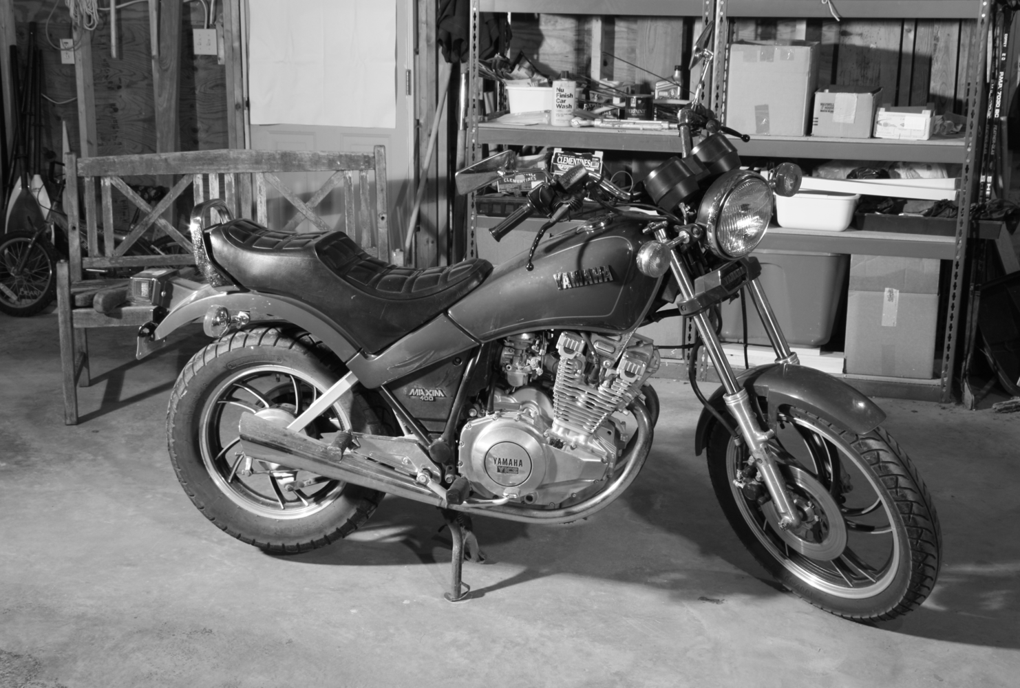
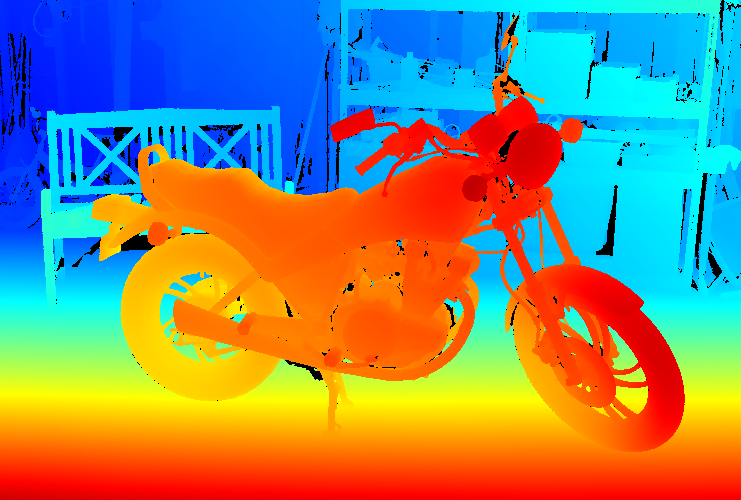
In the first experiment, we evaluate the practical performance of our proposed dynamic programming algorithms for minimizing the convex and nonconvex total variation subject to nonconvex piecewise linear unaries. For this, we consider different sizes of the stereo image pair and recorded the average time of computing the solutions of the horizontal lines during the first iteration of the algorithm. The number of break points is kept constant in all problems. The worst-case complexity for solving one problem of size $n$ is $O(n^{2})$ in case of convex total variation and exponential in case of nonconvex truncated total variation. The resulting timings are presented in Fig. 10. One can clearly see that the practical performance of the algorithm is significantly better than the theoretical worst-case complexities (see Sec. 3).

Figure 10: Evaluation of the practical performance of the proposed dynamic programming algorithm for minimizing 1D total variation subject to nonconvex piecewise linear unaries and using different sizes

n

. The practical performance for both convex total variation (TV) and nonconvex truncated total variation (TTV) is significantly better compared to the theoretical worst-case complexities presented in Sec. 3.

In our second experiment, we conduct exactly the same stereo experiment as in [9]. However, instead of computing the globally optimal solution by means of a lifting approach in 3D, we directly solve the nonconvex 2D Lagrangian problem. We use either convex total variation (TV) or truncated total variation (TTV) where we set the truncation value to be $C=10$ . The primal variables $x_{h,v}$ are initialized by the solutions of the 1D problems (assuming no coupling between the horizontal and vertical chains).

Fig. 11 shows a comparison between our proposed Lagrangian decomposition and the globally optimal solution obtained from [9]. Observe that the primal energy of the Lagrangian decomposition method quickly decreases during the first iterations. Suprisingly, we can approach the lower bound up to a very small error after a larger number of iterations. We also plot the color coded disparity maps corresponding to the average solution $\bar{x}^{k}=(x_{h}^{k}+x_{v}^{k})/2$ . While the solution after the first iteration still shows some streaking artifacts, the solution obtained after only $10$ iterations is visually almost identical to the globally optimal solution.

Fig. 12 finally shows a comparison between convex TV and nonconvex truncated TV using a truncation value of $C=10$ . We also decreased the strength of the data term by a factor of two in order to account for the less strong regularization of the TTV. One can see that the TTV solution yields sharper discontinuities (for example at the front wheel) and also preserves smaller details (fork tubes). It is also a bit more sensitive for outliers in the solution, which however can be removed by some post-processing procedure.

6 Conclusion

In this paper we proposed dynamic programming algorithms for minimizing the total variation subject to different pointwise data terms on trees. We considered general nonconvex piecewise linear data terms, convex piecewise linear (and quadratic) data terms and convex quadratic data terms.

In case of quadratic data terms, the resulting dynamic programming algorithm has a linear complexity in the signal length and can be seen as a generalization of Johnson’s method [23] to weighted total variation. In case of convex piecewise linear data terms, our dynamic programming algorithm has a worst case complexity of $O(n\log\log n)$ which improves the currently best performing algorithm [14]. In case of convex piecewise quadratic unaries we obtain an algorithm with a slightly worse complexity of $O(n\log n)$ but this algorithm turns out to be useful for computing proximity operators with respect to 1D TV- $\ell_{1}$ energies. Finally, in case of nonconvex piecewise linear unaries, we obtain a worst-case complexity of $O(n^{2})$ which turns out to be useful for approximately solving 2D stereo problems. We evaluated the dynamic programming algorithms by utilizing them as basic building blocks in primal-dual block decomposition algorithms for minimizing 2D total variation models. Our numerical experiments show the efficiency of the proposed algorithms.

In our block decomposition algorithms all 1D subproblems can be solved simultaneously, which clearly offers a lot of potential for parallelization and hence a speedup of the algorithms. We will pursue this direction in our future work.

Appendix A Proof of Proposition 2

It suffices to prove the claim for $m=2$ ; the general claim will then follow by induction. Denote $s=h\otimes g$ ; we need to show that $h^{2}=s(y)$ for all $y\in\mathbb{R}$ , where $h^{1}=h\otimes g^{1}$ and $h^{2}=h^{1}\otimes g^{2}$ .

Proof of $h^{2}(y)\leq s(y)$

First, observe that $h^{2}(z)\leq h^{1}(z)\leq h(z)$ for any $z$ since $g^{1}(0)=g^{2}(0)=0$ . For any $x$ we have

	$\displaystyle h^{2}(y)$	$\displaystyle\leq$	$\displaystyle h^{1}(y)\leq h(x)+g^{1}(y-x)$
	$\displaystyle h^{2}(y)$	$\displaystyle\leq$	$\displaystyle h^{1}(x)+g^{2}(y-x)=h(x)+g^{2}(y-x)$

and so

\displaystyle h^{2}(y)

\displaystyle\leq

\displaystyle h(x)+\min_{k\in\{1,2\}}g^{k}(y-x)=h(x)+g(y-x)

Therefore, $h^{2}(y)\leq\min_{x}[h(x)+g(y-x)]=s(y)$ .

Proof of $h^{2}(y)\geq s(y)$

For any $x,x^{\prime}$ we have

	$\displaystyle s(y)$	$\displaystyle\!\!\leq\!\!$	$\displaystyle h(x)+g(y-x)\;\leq\;h(x)+[g(x^{\prime}-x)+g(y-x^{\prime})]$
		$\displaystyle\!\!\leq\!\!$	$\displaystyle h(x)+g^{1}(x^{\prime}-x)+g^{2}(y-x^{\prime})$

where the second inequality holds by the triangle inequality (9). Therefore,

	$\displaystyle s(y)$	$\displaystyle\!\!\leq\!\!$	$\displaystyle\min_{x,x^{\prime}}[[h(x)+g^{1}(x^{\prime}-x)]+g^{2}(y-x^{\prime})]$
		$\displaystyle\!\!=\!\!$	$\displaystyle\min_{x^{\prime}}[h^{1}(x^{\prime})+g^{2}(y-x^{\prime})]\;=\;h^{2}(y)$

Mapping $\pi$

It remains to prove that mapping $\pi=\pi^{1}\circ\pi^{2}$ corresponds to min-convolution $h^{2}=h\otimes g$ . Let $x^{\prime}=\pi^{2}(y)$ and $x=\pi^{1}(x^{\prime})$ , then $h^{2}(y)=h^{1}(x^{\prime})+g^{2}(y-x^{\prime})$

$\displaystyle h^{2}(y)$	$\displaystyle\!\!=\!\!$	$\displaystyle h^{1}(x^{\prime})+g^{2}(y-x^{\prime})$
	$\displaystyle\!\!=\!\!$	$\displaystyle[h(x)+g^{1}(x^{\prime}-x)]+g^{2}(y-x^{\prime})$
	$\displaystyle\!\!\geq\!\!$	$\displaystyle h(x)+g(x^{\prime}-x)+g(y-x^{\prime})\geq h(x)+g(y-x)$

(the last inequality is again by (9)). The inequality $h(x)+g(y-x)\leq h^{2}(y)$ means that $x\in\argmin_{x}[h(x)+g(y-x)]$ .

Appendix B Proof of Proposition 3

Suppose that we are given positive numbers $b_{1},\ldots,b_{N}$ . We will construct a chain instance with $n=2N$ nodes such that values $\lambda^{-}_{ij}$ will give the input numbers in a sorted order. This will imply the claim since sorting requires at least $\Omega(n\log n)$ comparisons in the worst case [11].

The unary terms for nodes $i=1,\ldots,N$ nodes are given by $g_{i}(z)=\begin{cases}0&\mbox{if }z\leq b_{i}\\ 1&\mbox{if }z>b_{i}\end{cases}$ . The unary terms for nodes $i=N+1,\ldots,n$ are zeros. The weights for edges $(i,j)\in E$ are set as follows: $w^{-}_{ij}=0$ for all edges, $w^{+}_{ij}=N+1$ if $i<N$ , and $w^{+}_{ij}=2N-i-\frac{1}{2}$ if $i\geq N$ .

Let us sort numbers $b_{1},\ldots,b_{N}$ in the non-decreasing order, and denote the resulting sequence as $(c_{1},\ldots,c_{N})$ . It can be checked that $\lambda^{+}_{ij}=c_{2N-i}$ for $i=N,\ldots,2N-1$ .

Appendix C Proof of Proposition 4

First note that each problem is reduced to solving a finite amount of subproblems of the same type (recall that both $V_{0}$ and $V_{1}$ are unions of chains). Let $P_{1}^{0}$ stand for the original problem and inductively for $i\geq 1$ , let $P^{i}_{1}$ , …, $P^{i}_{k_{i}}$ be all the (direct) subproblems of the problems $P^{i-1}_{1}$ , …, $P^{i-1}_{k_{i-1}}$ . Also, let $\lambda(P)$ , $n(P)$ be the number of breakpoints and the number of nodes in subproblem $P$ , respectively. It follows by induction on $i$ that:

•

$\sum_{k}\lambda(P^{i}_{k})\leq|\Lambda|$ for each $i\geq 0$ .
•

$\sum_{k}n(P^{i}_{k})\leq n$ for each $i\geq 0$ .
•

$\lambda(P^{i}_{k})\leq|\Lambda|/2^{i}$ for each $i\geq 0$ and $k\geq 1$ and hence $i$ is $O(\log n)$ .

Since the complexity of dividing problem $P$ into subproblems is $O(\lambda(P)+n(P))$ as described in Section 4 we now compute the total complexity as

	$\displaystyle\sum_{i}\sum_{k}O(\lambda(P^{i}_{k})+n(P^{i}_{k}))$	$\displaystyle\!\!\!=\!\!\!$	$\displaystyle\sum_{i}O\left(\sum_{k}\lambda(P^{i}_{k})+n(P^{i}_{k})\right)$
		$\displaystyle\!\!\!=\!\!\!$	$\displaystyle\sum_{i}O(n)\subset O(n\log n).$

Appendix D Proof of Proposition 6

We use the same strategy to compute the complexity of the recursive algorithm as in Section C. Let $P^{0}_{1}$ be the original problem and inductively for $i\geq 1$ , let $P^{i}_{1}$ , …, $P^{i}_{k_{i}}$ be all the (direct) subproblems of the problems $P^{i-1}_{1}$ , …, $P^{i-1}_{k_{i-1}}$ . Let $\lambda(P)$ , ${\cal U}(P)$ , and ${\cal E}(P)$ be the sizes of the sets $\Lambda$ , ${\cal U}$ , and ${\cal E}$ of problem $P$ , respectively.

We claim that:

•

$\sum_{k}{\cal U}(P^{i}_{k})$ is $O(|{\cal U}|)$ for each $i\geq 0$ .
•

$\sum_{k}{\cal E}(P^{i}_{k})$ is $O(|{\cal E}|)$ for each $i\geq 0$ .
•

$\lambda(P^{i}_{k})\leq|\Lambda|\cdot(3/4)^{i}$ for each $i\geq 0$ and $k\geq 1$ and hence $i$ is $O(\log n)$ .

Since the total number of added vertices (or cut edges) is at most $|{\cal U}|$ (or $|{\cal E}|$ ), the first two statements follow immediately from induction on $i$ . For the third statement recall that the value $\lambda$ was chosen so that no more than $3/4$ breakpoints can end up in any of the sets $\Lambda^{+}=\{\lambda^{\prime}\in\Lambda:\lambda^{\prime}>\lambda\}$ , $\Lambda^{-}=\{\lambda^{\prime}\in\Lambda:\lambda^{\prime}<\lambda\}$ . Since for each subproblem the set of breakpoints is a subset of one of $\Lambda^{+}$ , $\Lambda^{-}$ the third statement follows again from induction on $i$ .

Since the complexity of dividing problem $P$ into subproblems is $O(({\cal U}(P)+{\cal E}(P))\log m)$ , we compute the entire complexity as

	$\displaystyle\sum_{i}\sum_{k}O(({\cal U}(P^{i}_{k})+{\cal E}(P^{i}_{k}))\log m)$
	$\displaystyle\quad=\sum_{i}O\left(\left(\sum_{k}{\cal U}(P^{i}_{k})+{\cal E}(P^{i}_{k})\right)\log m\right)$
	$\displaystyle\quad=\sum_{i}O((\|{\cal U}\|+\|{\cal E}\|)\log m)\subset O(n\log n\log n).$

References

[1] M. D. Atkinson, J. R. Sack, N. Santoro, and T. Strothotte. Min-max heaps and generalized priority queues. Communications of the ACM, 29(10):996–1000, 1986.
[2] Á. Barbero and S. Sra. Modular proximal optimization for multidimensional total-variation regularization. Technical report, arXiv:1411.0589, 2014.
[3] A. Beck and M. Teboulle. A fast iterative shrinkage-thresholding algorithm for linear inverse problems. SIAM J. Imaging Sci., 2(1):183–202, 2009.
[4] R. Bellman and W. Karush. Mathematical programming and the maximum transform. J. Soc. Indust. and Appl. Math., 10(3):550–567, 1962.
[5] J. P. Boyle and R. L. Dykstra. A method for finding projections onto the intersection of convex sets in Hilbert spaces. In Advances in order restricted statistical inference (Iowa City, Iowa, 1985), volume 37 of Lecture Notes in Statist., pages 28–47. Springer, Berlin, 1986.
[6] A. Chambolle. Total variation minimization and a class of binary MRF models. In EMMCVPR, pages 136–152, November 2005.
[7] A. Chambolle and T. Pock. A first-order primal-dual algorithm for convex problems with applications to imaging. Journal of Mathematical Imaging and Vision, 40(1):120–145, 2011.
[8] A. Chambolle and T. Pock. On the ergodic convergence rates of a first-order primal-dual algorithm. Mathematical Programming, pages 1–35, 2015. online first.
[9] A. Chambolle and T. Pock. A remark on accelerated block coordinate descent for computing the proximity operators of a sum of convex functions. SMAI Journal of Computational Mathematics, 1:29–54, 2015.
[10] Laurent Condat. A direct algorithm for 1D total variation denoising. IEEE Signal Proc. Letters, 20(11):1054–1057, 2013.
[11] Thomas H. Cormen, Charles E. Leiserson, Ronald L. Rivest, and Clifford Stein. Introduction to Algorithms. MIT Press, third edition, 2009.
[12] J. Darbon and M. Sigelle. Image restoration with discrete constrained total variation part I: Fast and exact optimization. J. of Math. Imaging and Vision, 26(3):261–276, 2006.
[13] P. L. Davies and A. Kovac. Local extremes, runs, strings and multiresolution. The Annals of Statistics, 29(1):1–65, 2001.
[14] L. Dümbgen and A. Kovac. Extensions of smoothing via taut strings. Electron. J. Statist., 3:41–75, 2009.
[15] M. J. Eisner and D. G. Severence. Mathematical techniques for efficient record segmentation in large shared databases. J. ACM, 23(4):619–635, October 1976.
[16] P. Felzenszwalb and D. Huttenlocher. Distance transforms of sampled functions. Theory of Computing, 8(19), 2012.
[17] P. Felzenszwalb and R. Zabih. Dynamic programming and graph algorithms in computer vision. PAMI, 33(4):721–740, 2011.
[18] M. L. Fredman and R. E. Tarjan. Fibonacci heaps and their uses in improved network optimization algorithms. J. of the ACM, 34(3):596–615, 1987.
[19] M. Grasmair. The equivalence of the taut string algorithm and BV-regularization. Journal of Mathematical Imaging and Vision, 27(1):59–66, 2007.
[20] William A. Greene. k-way merging and k-ary sorts. In Proceedings of the 31-st Annual ACM Southeast Conference, pages 127–135, 1993.
[21] W. Hinterberger, M. Hintermüller, K. Kunisch, M. von Oehsen, and O. Scherzer. Tube methods for BV regularization. Journal of Mathematical Imaging and Vision, 19(3):219–235, 2003.
[22] D. S. Hochbaum. An efficient algorithm for image segmentation, Markov Random Fields and related problems. J. ACM, 48:2:686–701, July 2001.
[23] N. A. Johnson. A dynamic programming algorithm for the fused lasso and $l_{0}$ -segmentation. J. Computational and Graphical Statistics, 2013.
[24] E. Mammen and S. van de Geer. Locally adaptive regression splines. The Annals of Statistics, 25(1):387–413, 1997.
[25] P. Maragos. Slope transforms: Theory and application to nonlinear signal processing. IEEE Trans. on Signal Processing, 43(4):864–877, 1995.
[26] K. Murota. Discrete Convex Analysis. SIAM Monographs on Discrete Mathematics and Applications, Vol. 10, 2003.
[27] L. Rudin, S. J. Osher, and E. Fatemi. Nonlinear total variation based noise removal algorithms. Physica D, 60:259–268, 1992. [also in Experimental Mathematics: Computational Issues in Nonlinear Science (Proc. Los Alamos Conf. 1991)].
[28] D. Scharstein, H. Hirschmüller, Y. Kitajima, G. Krathwohl, N. Nesic, X. Wang, and P. Westling. High-resolution stereo datasets with subpixel-accurate ground truth. In German Conference on Pattern Recognition (GCPR 2014), Münster, Germany, September 2014.
[29] G. Steidl, J. Weickert, T. Brox, P. Mrazek, and M. Welk. On the equivalence of soft wavelet shrinkage, total variation diffusion, total variation regularization, and SIDEs. SIAM J. Numer. Anal., 42(2):686–713, 2004.
[30] B. A. Zalesky. Network flow optimization for restoration of images. J. Appl. Math., 2(4):199–218, 2002.

Total variation on a tree

Abstract

1 Introduction

Non-convex case

Convex case

1.1 Related work

Non-convex case

Convex case on general graphs

Convex case on chains

1.2 Applications

2 Preliminaries

Min-convolution

Dynamic Programming

Proposition 1.

Proof.

3 Non-convex case

Lemma 1.

Lemma 2.

Corollary 1.

Proof.

3.1 Proof of Lemma 1

3.2 Proof of Lemma 2

Proposition 2.

Computing h⊗fi​j1h\otimes f^{1}_{ij}

Computing h⊗fi​j2h\otimes f^{2}_{ij}

Computing h⊗fi​j3h\otimes f^{3}_{ij}

3.3 Extensions

4 Convex case

4.1 Quadratic unaries on a chain: O⁡(n)O(n) algorithm

Forward pass

Backward pass

4.2 Piecewise-quadratic unaries: O⁡(n​log⁡n)O(n\log n) algorithm

Piecewise-linear unaries on a chain

Extension to trees

Extension to piecewise-quadratic unaries

4.3 Piecewise-linear unaries on a chain: O⁡(n​log⁡log​n)O(n\log\log n) algorithm

Proposition 3.

Theorem 1 ([22]).

Proposition 4.

Contraction

Proposition 5.

Divide-and-conquer algorithm

Proposition 6.

Remark 1

5 Application examples

5.1 TV-ℓ2\ell_{2} image restoration

5.2 TV-ℓ1\ell_{1} image restoration

5.3 TV-nonconvex

6 Conclusion

Appendix A Proof of Proposition 2

Proof of h2​(y)≤s​(y)h^{2}(y)\leq s(y)

Proof of h2​(y)≥s⁡(y)h^{2}(y)\geq s(y)

Mapping π\pi

Appendix B Proof of Proposition 3

Appendix C Proof of Proposition 4

Appendix D Proof of Proposition 6

References

Computing $h\otimes f^{1}_{ij}$

Computing $h\otimes f^{2}_{ij}$

Computing $h\otimes f^{3}_{ij}$

4.1 Quadratic unaries on a chain: $O(n)$ algorithm

4.2 Piecewise-quadratic unaries: $O(n\log n)$ algorithm

4.3 Piecewise-linear unaries on a chain: $O(n\log\log n)$ algorithm

5.1 TV- $\ell_{2}$ image restoration

5.2 TV- $\ell_{1}$ image restoration

Proof of $h^{2}(y)\leq s(y)$

Proof of $h^{2}(y)\geq s(y)$

Mapping $\pi$