Globally Optimal Crowdsourcing Quality Management

Akash Das Sarma

Aditya G. Parameswaran

Jennifer Widom Address: Stanford University Email: akashds@stanford.edu Address: University of Illinois (UIUC) Email: adityagp@illinois.edu Address: Stanford University Email: widom@cs.stanford.edu

Abstract

We study crowdsourcing quality management, that is, given worker responses to a set of tasks, our goal is to jointly estimate the true answers for the tasks, as well as the quality of the workers. Prior work on this problem relies primarily on applying Expectation-Maximization (EM) on the underlying maximum likelihood problem to estimate true answers as well as worker quality. Unfortunately, EM only provides a locally optimal solution rather than a globally optimal one. Other solutions to the problem (that do not leverage EM) fail to provide global optimality guarantees as well.

In this paper, we focus on filtering, where tasks require the evaluation of a yes/no predicate, and rating, where tasks elicit integer scores from a finite domain. We design algorithms for finding the global optimal estimates of correct task answers and worker quality for the underlying maximum likelihood problem, and characterize the complexity of these algorithms. Our algorithms conceptually consider all mappings from tasks to true answers (typically a very large number), leveraging two key ideas to reduce, by several orders of magnitude, the number of mappings under consideration, while preserving optimality. We also demonstrate that these algorithms often find more accurate estimates than EM-based algorithms. This paper makes an important contribution towards understanding the inherent complexity of globally optimal crowdsourcing quality management.

1 Introduction

Crowdsourcing [8] enables data scientists to collect human-labeled data at scale for machine learning algorithms, including those involving image, video, or text analysis. However, human workers often make mistakes while answering these tasks. Thus, crowdsourcing quality management, i.e., jointly estimating human worker quality as well as answer quality—the probability of different answers for the tasks—is essential. While knowing the answer quality helps us with the set of tasks at hand, knowing the quality of workers helps us estimate the true answers for future tasks, and in deciding whether to hire or fire specific workers.

In this paper, we focus on rating tasks, i.e., those where the answer is one from a fixed set of ratings $\in\{1,2,\ldots,R\}$ . This includes, as a special case, filtering tasks, where the ratings are binary, i.e., $\{0,1\}$ . Consider the following example: say a data scientist intends to design a sentiment analysis algorithm for tweets. To train such an algorithm, she needs a training dataset of tweets, rated on sentiment. Each tweet needs to be rated on a scale of $\{1,2,3\}$ , where $1$ is negative, $2$ is neutral, and $3$ is positive. A natural way to do this is to display each tweet, or item, to human workers hired via a crowdsourcing marketplace like Amazon’s Mechanical Turk [1], and have workers rate each item on sentiment from 1—3. Since workers may answer these rating tasks incorrectly, we may have multiple workers rate each item. Our goal is then to jointly estimate sentiment of each tweet and the accuracy of the workers.

Standard techniques for solving this estimation problem typically involve the use of the Expectation-Maximization (EM). Applications of EM, however, provide no theoretical guarantees. Furthermore, as we will show in this paper, EM-based algorithms are highly dependent on initialization parameters and can often get stuck in undesirable local optima. Other techniques for optimal quality assurance, some specific to only filtering [5, 9, 14], are not provably optimal either, in that they only give bounds on the errors of their estimates, and do not provide the globally optimal quality estimates. We cover other related work in the next section.

In this paper, we present a technique for globally optimal quality management, that is, finding the maximum likelihood item (tweet) ratings, and worker quality estimates. If we have $500$ tweets and $3$ possible ratings, the total number of mappings from tweets to ratings is $3^{500}$ . A straightforward technique for globally optimal quality management is to simply consider all possible mappings, and for each mapping, infer the overall likelihood of that mapping. (It can be shown that the best worker error rates are easy to determine once the mapping is fixed.) The mapping with the highest likelihood is then the global optimum.

However, the number of mappings even in this simple example, $3^{500}$ , is very large, therefore making this approach infeasible. Now, for illustration, let us assume that workers are indistinguishable, and they all have the same quality (which is unknown). It is well-understood that at least on Mechanical Turk, the worker pool is constantly in flux, and it is often hard to find workers who have attempted enough tasks in order to get robust estimates of worker quality. (Our techniques also apply to a generalization of this case.)

To reduce this exponential complexity, we use two simple, but powerful ideas to greatly prune the set of mappings that need to be considered, from $3^{500}$ , to a much more manageable number. Suppose we have 3 ratings for each tweet—a common strategy in crowdsourcing is to get a small, fixed number of answers for each question. First, we hash “similar” tweets that receive the same set of worker ratings into a common bucket. As shown in Figure 1, suppose that 300 items each receive three ratings of $3$ (positive), 100 items each receive one rating of 1, one rating of 2 and one rating of 3, and 100 items each receive three ratings of $1$ . That is, we have three buckets of items, corresponding to the worker answer sets $B_{1}=\{3,3,3\}$ , $B_{2}=\{1,2,3\}$ , and $B_{3}=\{1,1,1\}$ . We now exploit the intuition that if two items receive the same set of worker responses they should be treated identically. We therefore only consider mappings that assign the same rating to all items (tweets) within a bucket. Now, since in our example, we only have 3 buckets each of which can be assigned a rating of 1,2, or 3, we are left with just $3^{3}=27$ mappings to consider.

Refer to caption — Figure 1: Mapping Example

Next, we impose a partial ordering on the set of buckets based on our belief that items in certain buckets should receive a higher final rating than items in other buckets. Our intuition is simple: if an item received “higher” worker ratings than another item, then its final assigned rating should be higher as well. In this example, our partial ordering, or dominance ordering on the buckets is $B_{1}\geq B_{2}\geq B_{3}$ , that is, intuitively items which received all three worker ratings of $3$ should not have a true rating smaller than items in the second or third buckets where items receive lower ratings. This means that we can further reduce our space of $27$ remaining mappings by removing all those mappings that do not respect this partial ordering. The number of such remaining mappings is 10, corresponding to when all items in the buckets $(B_{1},B_{2},B_{3})$ are mapped respectively to ratings $(3,3,3)$ , $(3,3,2)$ , $(3,3,1)$ , $(3,2,2)$ , $(3,2,1)$ , $(3,1,1)$ , $(2,2,2)$ , $(2,2,1)$ , $(2,1,1)$ , and $(1,1,1)$ .

In this paper, we formally show that restricting the mappings in this way does not take away from the optimality of the solution; i.e., there exists a mapping with the highest likelihood that obeys the property that all items with same scores are mapped to the same rating, and at the same time obeys the dominance ordering relationship as described above.

Our list of contributions are as follows:

$\bullet$

We develop an intuitive algorithm based on simple, but key insights that finds a provably optimal maximum likelihood solution to the problem of jointly estimating true item labels and worker error behavior for crowdsourced filtering and rating tasks. Our approach involves reducing the space of potential ground truth mappings while preserving optimality, enabling an exhaustive search on an otherwise prohibitive domain.
$\bullet$

Although we primarily focus on and initially derive our optimality results for the setting where workers independently draw their responses from a common error distribution, we also propose generalizations to harder settings, for instance, when workers are known to come from distinct classes with separate error distributions. That said, even the former setting is commonly used in practice, and represents a significant first step towards understanding the nature and complexity of exact globally optimal solutions for this joint estimation problem.
$\bullet$

We perform experiments on synthetic and real datasets to evaluate the performance of our algorithm on a variety of different metrics. Though we optimize for likelihood, we also test the accuracy of predicted item labels and worker response distributions. We show that our algorithm also does well on these other metrics. We test our algorithm on a real dataset where our assumptions about the worker model do not necessarily hold, and show that our algorithm still yields good results.

1.1 Related Literature

Crowdsourcing is gaining importance as a platform for a variety of different applications where automated machine learning techniques don’t always perform well, e.g., filtering [17] or labeling [18, 20, 24] of text, images, or video, and entity resolution [2, 22, 23, 25]. One crucial problem in crowdsourced applications is that of worker quality: since human workers often make mistakes, it is important to model and characterize their behavior in order to aggregate high-quality answers.

EM-based joint estimation techniques. We study the particular problem of jointly estimating hidden values (item ratings) and a related latent set of parameters (worker error rates) given a set of observed data (worker responses). A standard machine learning technique for estimating parameters with unobserved latent variables is Expectation Maximization [10]. There has been significant work in using EM-based techniques to estimate true item values and worker error rates, such as [7, 21, 26], and subsequent modifications using Bayesian techniques [3, 16]. In [19], the authors use a supervised learning approach to learn a classifier and the ground truth labels simultaneously. In general, these machine learning based techniques only provide probabilistic guarantees and cannot ensure optimality of the estimates. We solve the problem of finding a global, provably maximum likelihood solution for both the item values and the worker error rates. That said, our worker error model is simpler than the models considered in these papers—in particular, we do not consider worker identities or difficulties of individual items. While we do provide generalizations to our approach that relax some of these assumptions, they can be inefficient in practice. However, we study this simpler model in more depth, providing optimality guarantees. Since our work represents the first providing optimality guarantees (even for a restricted setting), it represents an important step forward in our understanding of crowdsourcing quality management. Furthermore, anecdotally, even the simpler model is commonly used for platforms like Mechanical Turk, where the workers are fleeting.

Other techniques with no guarantees. There has been some work that adapts techniques different from EM to solve the problem of worker quality estimation. For instance, Chen et al. [4] adopts approximate Markov Decision Processes to perform simultaneous worker quality estimation and budget allocation. Liu et al. [15] uses variational inference for worker quality management on filtering tasks (in our case, our techniques apply to both filtering and rating). Like EM-based techniques, these papers do not provide any theoretical guarantees.

Weaker guarantees. There has been a lot of recent work on providing partial probabilistic guarantees or asymptotic guarantees on accuracies of answers or worker estimates, for various problem settings and assumptions, and using various techniques. We first describe the problem settings adopted by these papers, then their solution techniques, and then describe their partial guarantees.

The most general problem setting adopted by these papers is identical to us (i.e., rating tasks with arbitrary bipartite graphs connecting workers and tasks) [27]; most papers focus only on filtering [5, 9, 14], or operate only when the graph is assumed to be randomly generated [13, 14]. Furthermore, most of these papers assume that the false positive and false negative rates are the same.

The papers draw from various techniques, including just spectral methods [5, 9], just message passing [14], a combination of spectral methods and message passing [13], or a combination of spectral methods and EM [27].

In terms of guarantees, most of the papers provide probabilistic bounds [5, 13, 14, 27], while some only provide asymptotic bounds [9]. For example, Dalvi et al. [5], which represents the state of the art over multiple papers [9, 13, 14], show that under certain assumptions about the graph structure (depending on the eigenvalues) the error in their estimates of worker quality is lower than some quantity with probability greater than $1-\delta$ .

Thus, overall, all the work discussed so far provides probabilistic guarantees on their item value predictions, and error bound guarantees on their estimated worker qualities. In contrast, we consider the problem of finding a global maximum likelihood estimate for the correct answers to tasks and the worker error rates.

Other related papers. Joglekar et al. [12] consider the problem of finding confidence bounds on worker error rates. Our paper is complementary to theirs in that, while they solve the problem of obtaining confidence bounds on the worker error rates, we consider the problem of finding the maximum likelihood estimates to the item ground truth and worker error rates.

Zhou et al. [28, 29] use minimax entropy to perform worker quality estimation as well as inherent item difficulty estimation; here the inherent item difficulty is represented as a vector. Their technique only applies when the number of workers attempting each task is very large; here, overfitting (given the large number of hidden parameters) is no longer a concern. For cases where the number of workers attempting each task is in the order of 50 or 100 (highly unrealistic in practical applications), the authors demonstrate that the scheme outperforms vanilla EM.

Summary. In summary, at the highest level, our work differs from all previous work in its focus on finding a globally optimal solution to the maximum likelihood problem. We focus on a simpler setting, but do so in more depth, representing significant progress in our understanding of global optimality. Our globally optimal solution uses simple and intuitive insights to reduce the search space of possible ground truths, enabling exhaustive evaluation. Our general framework leaves room for further study and has the potential for more sophisticated algorithms that build on our reduced space.

2 Preliminaries

We start by introducing some notation, and then describe the general problem that we study in this paper; specific variants will be considered in subsequent sections.

Items and Rating Questions. We let ${\bf I}$ be a set of $|\mathbf{I}|=n$ items. Items could be, for example, images, videos, or pieces of text.

Given an item $I\in{\bf I}$ , we can ask a worker $w$ to answer a rating question on that item. That is, we ask a worker: What is your rating $r$ for the item $I$ ?. We allow workers to rate the item with any value $\in\{1,2,\ldots,R\}$ .

Example 2.1

Recall our example application from Section 1, where we have $R=3$ and workers can rate tweets as being negative ( $r=1$ ), neutral ( $r=2$ ), or positive ( $r=3$ ). Suppose we have two items, $\mathbf{I}=\{I_{1},I_{2}\}$ where $I_{1}$ is positive, or has a true rating of 3, and $I_{2}$ is neutral, or has a true rating of 2.

Response Set. We assume that each item $I$ is shown to $m$ arbitrary workers, and therefore receives $m$ ratings $\in[1,R]$ . We denote the set of ratings given by workers for item $I$ as $M(I)$ and write $M(I)=(v_{R},v_{R-1},\ldots,v_{1})$ if item $I\in\mathbf{I}$ receives $v_{i}$ responses of rating “ $i$ ” across workers, $1\leq i\leq R$ . Thus, $\overset{R}{\underset{i=1}{\sum}}v_{i}=m$ . We call $M(I)$ the response set of $I$ , and $M$ the worker response set in general.

Continuing with Example 2.1, suppose we have $m=2$ workers rating each item on the scale of $\{1,2,3\}$ . Let $I_{1}$ receive one worker response of $2$ and one worker response of $3$ . Then, we write $M(I_{1})=(1,1,0)$ . Similarly, if $I_{2}$ receives one response of $3$ and one response of $1$ , then we have $M(I_{2})=(1,0,1)$ .

Modeling Worker Errors. We assume that every item $I\in{\bf I}$ has a true rating in $[1,R]$ that is not known to us in advance. What we can do is estimate the true rating using the worker response set. To estimate the true rating, we need to be able to estimate the probabilities of worker errors.

We assume every worker draws their responses from a common (discrete) response probability matrix, $p$ , of size $R\times R$ . Thus, $p(i,j)$ is the probability that a worker rates an item with true value $j$ as having rating $i$ . Consider the following response probability matrix of the workers described in our example ( $R=3$ ):

p=\begin{bmatrix}0.7&0.1&0.2\\ 0.2&0.8&0.2\\ 0.1&0.1&0.6\end{bmatrix}

H ere, the $j^{th}$ column represents the different probabilities of worker responses when an item’s true rating is $j$ . Correspondingly, the $i^{th}$ row represents the probabilities that a worker will rate an item as $i$ . We have $p(1,1)=0.7,p(2,1)=0.2,p(3,1)=0.1$ meaning that given an item whose true rating is 1, workers will rate the item correctly with probability $0.7$ , give it a rating of 2 with probability 0.2, and give it a rating of 3 with probability 0.1. The matrix $p$ is in general not known to us. We aim to estimate both $p$ and the true ratings of items in ${\bf I}$ as part of our computation.

Note that we assume that every response to a rating question returned by every worker is independently and identically drawn from this matrix: thus, each worker responds to each rating question independently of other questions they may have answered, and other ratings for the same question given by other workers; and furthermore, all the workers have the same response matrix. In our example, we assume that all four responses (2 responses to each of $I_{1},I_{2}$ ) are drawn from this distribution. We recognize that assuming the same response matrix is somewhat stringent—we will consider generalizations to the case where we can categorize workers into classes (each with the same response matrix) in Section 5. That said, while our techniques can still indeed be applied when there are a large number of workers or worker classes with distinct response matrices, it may be impractical. Since our focus is on understanding the theoretical limits of global optimality for a simple case, we defer to future work fully generalizing our techniques to apply to workers with distinct response matrices, or when worker answers are not independent of each other.

Mapping and Likelihood We call a function $f:\mathbf{I}\rightarrow\{1,2,\ldots,R\}$ that assigns ratings to items a mapping. The set of actual ratings of items is also a mapping. We call that the ground truth mapping, $T$ . For Example 2.1, $T(I_{1})=3,T(I_{2})=2$ .

Our goal is to find the most likely mapping and worker response matrix given the response set $M$ . We let the probability of a specific mapping, $f$ , being the ground truth mapping, given the worker response set $M$ and response probability matrix $p$ be denoted by $\Pr(f|M,p)$ . Using Bayes rule, we have $\Pr(f|M,p)=k\Pr(M|f,p)$ , where $\Pr(M|f,p)$ is the probability of seeing worker response set $M$ given that $f$ is the ground truth mapping and $p$ is the true worker error matrix. Here, $k$ is the constant given by $k=\frac{\Pr(f)}{\Pr(M)}$ , where $\Pr(f)$ is the (constant) apriori probability of being the ground truth mapping and $\Pr(M)$ is the (constant) apriori probability of seeing worker response set $M$ . Thus, $\Pr(M|f,p)$ is the probability of workers providing the responses in $M$ , had $f$ been the ground truth mapping and $p$ been the true worker error matrix. We call this value the likelihood of the mapping-matrix pair, $f,p$ .

We illustrate this concept on our example. We have $M(I_{1})=(1,1,0)$ and $M(I_{2})=(1,0,1)$ . Let us compute the likelihood of the pair $f,p$ when $f(I_{1})=2,f(I_{2})=2$ and $p$ is the matrix displayed above. We have

\Pr(M|f,p)=\Pr(M(I_{1})|f,p)\Pr(M(I_{2})|f,p)

assuming that rating questions on items are answered independently. The quantity $\Pr(M(I_{1})|f,p)$ is the probability that workers drawing their responses from $p$ respond with $M(I_{1})$ to an item with true rating $f(I_{1})$ . Again, assuming independence of worker responses, this quantity can be written as the product of the probability of seeing each of the responses that $I_{1}$ receives. If $f$ is given as the ground truth mapping, we know that the probability of receiving a response of $i$ is $p(i,f(I_{1}))=p(i,2)$ . Therefore, the probability of seeing $M(1,1,0)$ , that is one response of $3$ and one response of $2$ , is $p(3,2)p(2,2)=0.1\times 0.8=0.08$ . Similarly, $\Pr(M(I_{2})|f,p)=p(3,2)\times p(1,2)=0.1\times 0.1=0.01$ . Combining all of these expressions, we have $\Pr(M|f,p)=0.01\times 0.08=8\times 10^{-4}$ .

Symbol	Explanation
$\mathbf{I}$	Set of items
$M$	Items-workers response set
$f$	Items-values mapping
$p$	Worker response probability matrix
$\Pr(M\|f,p)$	Likelihood of $(f,p)$
$m$	Number of worker responses per item
$T$	Ground truth mapping

Table 1: Notation Table

Thus, our goal can be restated as:

Problem 2.1 (Maximum Likelihood Problem)

Given $M,\mathbf{I}$ , find

\underset{f,p}{\arg\!\max}\Pr(M|f,p)

A naive solution would be to look at every possible mapping $f^{\prime}$ , compute $p^{\prime}=\underset{p}{\arg}\!\max\Pr(M|f^{\prime},p)$ and choose the $f^{\prime}$ maximizing the likelihood value $\Pr(M|f^{\prime},p^{\prime})$ . The number of such mappings, $R^{|\mathbf{I}|}$ , is however exponentially large.

We list our notation in Table 1 for ready reference.

3 Filtering Problem

Filtering can be regarded as a special case of rating where $R=2$ . We discuss it separately, first, because its analysis is significantly simpler, and at the same time provides useful insights that we then build upon for the generalization to rating, that is, to the case where $R>2$ . For example, consider the filtering task of finding all images of Barack Obama from a given set of images. For each image, we ask workers the question “is this a picture of Barack Obama”. Images correspond to items and the question “is this a picture of Barack Obama” corresponds to the filtering taskon each item. We can represent an answer of “no” to the question above by a score 0, and an answer of “yes” by a score 1. Each item $I\in\mathbf{I}$ now has an inherent true value in $\{0,1\}$ where a true value of 1 means that the item is one that satisfies the filter, in this case, the image is one of Barack Obama. Mappings here are functions $f:\mathbf{I}\rightarrow\{0,1\}$ .

Next, we formalize the filtering problem in Section 3.1, describe our algorithm in Section 3.2, prove a maximum likelihood result in Section 3.3 and evaluate our algorithm in Section 3.5.

3.1 Formalization

Given the response set $M$ , we wish to find the maximum likelihood mapping $f:\mathbf{I}\rightarrow\{0,1\}$ and $2\times 2$ response probability matrix, $p$ . For the filtering problem, each item has an inherent true value of either 0 or 1, and sees $m$ responses of 0 or 1 from different workers. If item $I$ receives $m-j$ responses of 1 and $j$ responses of 0, we can represent its response set with the tuple or pair $M(I)=(m-j,j)$ .

Consider a worker response probability matrix of $p=\begin{bmatrix}0.7&0.2\\ 0.3&0.8\end{bmatrix}$ . The first column represents the probabilities of worker responses when an item’s true rating is $0$ and the second column represents probabilities when an item’s true rating is $1$ . Given that all workers have the same response probabilities, we can characterize their response matrix by just the corresponding worker false positive (FP) and false negative (FN) rates, $e_{0}$ and $e_{1}$ . That is, $e_{0}=p(1,0)$ is the probability that a worker responds $1$ to an item whose true value is $0$ , and $e_{1}=p(0,1)$ is the probability that a worker responds $0$ to an item whose true value is $1$ . We have $p(1,1)=1-e_{1}$ and $p(0,0)=1-e_{0}$ . Here, we can describe the entire matrix $p$ with just the two values, $e_{0}=0.3$ and $e_{1}=0.2$ .

Filtering Estimation Problem. Let $M$ be the observed response set on item-set $\mathbf{I}$ . Our goal is to find

f^{*},e_{0}^{*},e_{1}^{*}=\underset{f,e_{0},e_{1}}{\arg\!\max}\Pr(M|f,e_{0},e_{1})

Here, $\Pr(M|f,e_{0},e_{1})$ is the probability of getting the response set $M$ , given that $f$ is the ground truth mapping and the true worker response matrix is defined by $e_{0},e_{1}$ .

Dependance of Response Probability Matrices on Mappings. Due to the probabilistic nature of our workers, for a fixed ground truth mapping $T$ , different worker error rates, $e_{0}$ and $e_{1}$ can produce the same response set $M$ . These different worker error rates, however have varying likelihoods of occurrence. This leads us to observe that worker error rates ( $e_{0},e_{1}$ ) and mapping functions ( $f$ ) are not independent and are related through any given $M$ . In fact, we show that for the maximum likelihood estimation problem, fixing a mapping $f$ enforces a maximum likelihood choice of $e_{0},e_{1}$ . We leverage this fact to simplify our problem from searching for the maximum likelihood tuple $f,e_{0},e_{1}$ to just searching for the maximum likelihood mapping, $f$ . Given a response set $M$ and a mapping, $f$ , we call this maximum likelihood choice of $e_{0},e_{1}$ as the parameter set of $f,M$ , and represent it as $\text{Params}(f,M)$ . The choice of $\text{Params}(f,M)$ is very intuitive and simple. We show that we just can estimate $e_{0}$ as the fraction of times a worker disagreed with $f$ on an item $I$ in $M$ when $f(I)=0$ , and correspondingly, $e_{1}$ as the fraction of times a worker responded $0$ to an item $I$ , when $f(I)=1$ . Under this constraint, we can prove that our original estimation problem,

\underset{f,e_{0},e_{1}}{\arg\!\max}\Pr(M|f,e_{0},e_{1})

simplifies to that of finding

\underset{f}{\arg\!\max}\Pr(M|f,e_{0}^{*},e_{1}^{*})

where $e_{0}^{*},e_{1}^{*}$ are the constants given by $\text{Params}(f,M)$ .

Example 3.1

Suppose we are given $4$ items $\mathbf{I}=\{I_{1},I_{2},I_{3},I_{4}\}$ with ground truth mapping $T=(T(I_{1}),T(I_{2}),T(I_{3}),T(I_{4}))=(1,0,1,1)$ .

Suppose we ask $m=3$ workers to evaluate each item and receive the following number of (“1”,“0”) responses for each respective item: $M(I_{1})=(3,0),M(I_{2})=(1,2),M(I_{3})=(2,1),M(I_{4})=(2,1)$ . Then, we can evaluate our worker false positive and false negative rates as described above: $e_{0}=\frac{0+1+1}{3+3+3}=\frac{2}{9}$ (from items $I_{1}$ , $I_{3}$ and $I_{4}$ ) and $e_{1}=\frac{1}{3}$ (from $I_{2}$ ).

We shall henceforth refer to $\Pr(M|f)=\Pr(M|f,\text{Params}(f,M))$ as the likelihood of a mapping $f$ . For now, we focus on the problem of finding the maximum likelihood mapping with the understanding that finding the error rates is straightforward given the mapping is fixed. In Section 3.4, we formally show that the problem of jointly finding the maximum likelihood response matrix and mapping can be solved by just finding the most likely mapping $f^{*}$ . The most likely triple $f,e_{0},e_{1}$ is then given by $f^{*},\text{Params}(f^{*},M)$ .

It is easy to calculate the likelihood of a given mapping. We have $\Pr(M|f)=\underset{I\in\mathbf{I}}{\prod}\Pr(M(I)|f,e_{0},e_{1})$ , where $e_{0},e_{1}=\text{Params}(f,M)$ and $\Pr(M(I)|f,e_{0},e_{1})$ is the probability of seeing the response set $M(I)$ on an item $I\in\mathbf{I}$ . Say $M(I)=(m-j,j)$ . Then, we have

\Pr(M(I)|f)=\begin{cases}(1-e_{1})^{m-j}e_{1}^{j}&\text{for }f(I)=1\\ e_{0}^{m-j}(1-e_{0})^{j}&\text{for }f(I)=0\\ \end{cases}

This can be evaluated in $O(m)$ for each $I\in\mathbf{I}$ by doing one pass over $M(I)$ . Thus, $\Pr(M|f)=\prod_{I\in\mathbf{I}}\Pr(M(I)|f)$ can be evaluated in $O(m|\mathbf{I}|)$ . We use this as a building block in our algorithm below.

3.2 Globally Optimal Algorithm

In this section, we describe our algorithm for finding the maximum likelihood mapping, given a response set $M$ on an item set $\mathbf{I}$ . A naive algorithm could be to scan all possible mappings, $f$ , calculating for each, $e_{0}^{*},e_{1}^{*}=\text{Params}(f,M)$ and the likelihood $\Pr(M|f,e_{0}^{*},e_{1}^{*})$ . The number of all possible mappings is, however, exponential in the number of items. Given $n=|\mathbf{I}|$ items, we can assign a value of either $0$ or $1$ to any of them, giving rise to a total of $2^{n}$ different mappings. This makes the naive algorithm prohibitively expensive.

Our algorithm is essentially a pruning based method that uses two simple insights (described below) to narrow the search for the maximum likelihood mapping. Starting with the entire set of $2^{n}$ possible mappings, we eliminate all those that do not satisfy one of our two requirements, and reduce the space of mappings to be considered to $O(m)$ , where $m$ is the number of worker responses per item. We then show that just an exhaustive evaluation on this small set of remaining mappings is still sufficient to find a global maximum likelihood mapping.

We illustrate our ideas on the example from Section 3.1, represented graphically in Figure 2. We will explain this figure below.

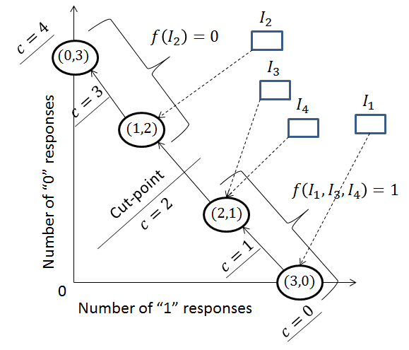
Bucketizing. Since we assume (for now) that all workers draw their responses from the same probability matrix $p$ (i.e., have the same $e_{0},e_{1}$ values), we observe that items with the exact same set of worker responses can be treated identically. This allows us to bucket items based on their observed response sets. Given that there are $m$ worker responses for each item, we have $m+1$ buckets, starting from $m$ “1” and zero “0” responses, down to zero “1” and $m$ “0” responses. We represent these buckets in Figure 2. The x-axis represents the number of $1$ responses an item receives and the y-axis represents the number of $0$ responses an item receives. Since every item receives exactly $m$ responses, all possible response sets lie along the line $x+y=m$ . We hash items into the buckets corresponding to their observed response sets. Intuitively, since all items within a bucket receive the same set of responses and are for all purposes identical, two items within a bucket should receive the same value. It is more reasonable to give both items a value of 1 or 0 than to give one of them a value of 1 and the other 0.

In our example (Figure 2), the set of possible responses to any item is $\{(3,0),(2,1),(1,2),(0,3)\}$ , where $(3-j,j)$ represents seeing $3-j$ responses of “1” and $j$ responses of “0”. We have $I_{1}$ in the bucket $(3,0)$ , $I_{3},I_{4}$ in the bucket (2,1), $I_{2}$ in the bucket $(1,2)$ , and an empty bucket $(0,3)$ . We only consider mappings, $f$ , where items in the same bucket are assigned the same value, that is, $f(I_{3})=f(I_{4})$ . This leaves $2^{4}$ mappings corresponding to assigning a value of 0/1 to each bucket. In general, given $m$ worker responses per item, we have $m+1$ buckets and $2^{m+1}$ mappings that satisfy our bucketizing condition. Although for this example $m+1=n$ , typically we have $m\ll n$ .

Dominance Ordering. Second, we observe that buckets have an inherent ordering. If workers are better than random, that is, if their false positive and false negative error rates are less than 0.5, we intuitively expect items with more “1” responses to be more likely to have true value $1$ than items with fewer “1” responses. Ordering buckets by the number of “1” responses, we have $(m,0)\rightarrow(m-1,1)\rightarrow\ldots\rightarrow(1,m-1)\rightarrow(0,m)$ , where bucket $(m-j,j)$ contains all items that received $m-j$ “1” responses and $j$ “0” responses. We eliminate all mappings that give a value of $0$ to a bucket with a larger number of “1” responses while assigning a value of $1$ to a bucket with fewer “1” responses. We formalize this intuition as a dominance relation, or ordering on buckets, $(m,0)>(m-1,1)>\ldots>(1,m-1)>(0,m)$ , and only consider mappings where dominating buckets receive a value not lower than any of their dominated buckets.

Let us impose this dominance ordering on our example. For instance, $I_{1}$ (three workers respond “1”) is more likely to have ground truth value “1”, or dominates, $I_{3},I_{4}$ , (two workers respond “1”), which in turn dominate $I_{2}$ . So, we do not consider mappings that assign a value of “0” to a $I_{1}$ and “1” to either of $I_{3},I_{4}$ . Figure 2 shows the dominance relation in the form of directed edges, with the source node being the dominating bucket and the target node being the dominated one. Combining this with our bucketizing idea, we discard all mappings which assign a value of “0” to a dominating bucket (say response set $(3,0)$ ) while assigning a value of “1” to one of its dominated buckets (say response set $(2,1)$ ).

Dominance-Consistent Mappings. We consider the space of mappings satisfying our above bucketizing and dominance constraints, and call them dominance-consistent mappings. We can prove that the maximum likelihood mapping from this small set of mappings is in fact a global maximum likelihood mapping across the space of all possible “reasonable” mappings: mappings corresponding to better than random worker behavior.

To construct a mapping satisfying our above two constraints, we choose a cut-point to cut the ordered set of response sets into two partitions. The corresponding dominance-consistent mapping then assigns value “1” to all (items in) buckets in the first (better) half, and value “0” to the rest. For instance, choosing the cut-point between response sets $(2,1)$ and $(1,2)$ in Figure 2 results in the corresponding dominance-consistent mapping, where $\{I_{1},I_{3},I_{4}\}$ , are mapped to “1”, while $\{I_{2}\}$ , is mapped to “0”. We have 5 different cut-points, $0,1,2,3,4$ , each corresponding to one dominance-consistent mapping. Cut-point 0 corresponds to the mapping where all items are assigned a value of 0 and cut-point 4 corresponds to the mapping where all items are assigned a value of 1. In particular, the figure shows the dominance-consistent mapping corresponding to the cut-point $c=2$ . In general, if we have $m$ responses to each item, we obtain $m+2$ dominance-consistent mappings.

Definition 3.1 (Dominance-consistent mapping $f^{c}$ )

For any cut-point $c\in 0,1,\ldots,m+1$ , we define the corresponding dominance-point mapping $f^{c}$ as

f^{c}(I)=\begin{cases}1&\text{if }M(I)\in\{(m,0),\ldots,(m-c+1,c-1)\}\\ 0&\text{if }M(I)\in\{(m-c,c),\ldots,(0,m)\}\\ \end{cases}

Our algorithm enumerates all dominance-consistent mappings, computes their likelihoods, and returns the most likely one among them. As there are $(m+2)$ mappings, each of whose likelihoods can be evaluated in $O(m|\mathbf{I}|)$ , (See Section 3.1) the running time of our algorithm is $O(m^{2}|\mathbf{I}|)$ .

Algorithm 1 Cut-point Algorithm

I:=\text{Input Item-set}

M:=\text{Input Response Set}

f:=\{\}

{Different dominance-consistent (mappings)}

e_{0}:=\{\}

{

e_{0}

rates corresponding to cut-functions}

e_{1}:=\{\}

{

e_{1}

rates corresponding to cut-functions}

Likelihood:=\{\}

{Likelihoods corresponding to cut-functions} {Enumerating across cut-points:}

7: for

c

\{0,1,\ldots,m+1\}

e_{0}[c],e_{1}[c]:=\text{Params}(f[c],M)

Likelihood[c]:=\Pr(M|f[c],e_{0}[c],e_{1}[c])

10: end for

11:

c^{*}:=\underset{c}{\arg\!\max}Likelihood[c]

12: RETURN

(f[c^{*}],e_{0}[c^{*}],e_{1}[c^{*}])

In the next section we prove that in spite of only searching the much smaller space of dominance-consistent mappings, our algorithm finds a global maximum likelihood solution.

3.3 Proof of Correctness

Reasonable Mappings. A reasonable mapping is one which corresponds to a better than random worker behavior. Consider a mapping $f$ corresponding to a false positive rate of $e_{0}>0.5$ (as given by $\text{Params}(f,M)$ ). This mapping is unreasonable because workers perform worse than random for items with value “0”. Given $\mathbf{I},M$ , let $f:\mathbf{I}\rightarrow\{0,1\}$ , with $e_{0},e_{1}=\text{Params}(f,M)$ be a mapping such that $e_{0}\leq 0.5$ and $e_{1}\leq 0.5$ . Then $f$ is a reasonable mapping. It is easy to show that all dominance-consistent mappings are reasonable mappings.

Now, we present our main result on the optimality of our algorithm. We show that in spite of only considering the local space of dominance-consistent mappings, we are able to find a global maximum likelihood mapping.

Theorem 3.1 (Maximum Likelihood)

We let $M$ be the given response set on the input item-set $\mathbf{I}$ . Let $\mathbf{F}$ be the set of all reasonable mappings and $\mathbf{F}^{dom}$ be the set of all dominance-consistent mappings. Then,

\max_{f^{*}\in\mathbf{F^{dom}}}\Pr(M|f^{*})=\max_{f\in\mathbf{F}}\Pr(M|f)

Proof 3.1

We divide our proof into steps. The first step describes the overall flow of the proof and provides the high level structure for the remaining steps. Step 1: Suppose $f$ is not a dominance-consistent mapping. Then, either it does not satisfy the bucketizing constraint, or it does not satisfy the dominance-constraint. We claim that if $f$ is reasonable, we can always construct a dominance-consistent mapping, $f^{*}$ such that $\Pr(M|f^{*})\geq\Pr(M|f)$ . Then, it trivially follows that $\max_{f^{*}\in\mathbf{F^{dom}}}\Pr(M|f^{*})=\max_{f\in\mathbf{F}}\Pr(M|f)$ . We show the construction of such an $f^{*}$ for every reasonable mapping $f$ in the following steps.

Step 2: (Dominance Inconsistency). Suppose $f$ does not satisfy the dominance constraint. Then, there exists at least one pair of items $I_{1},I_{2}$ such that $M(I_{1})>M(I_{2})$ and $f(I_{1})=0,f(I_{2})=1$ . Define mapping $f^{\prime}$ as follows:

f^{\prime}(I)=\begin{cases}f(I_{2})&\text{for }I=I_{1}\\ f(I_{1})&\text{for }I=I_{2}\\ f(I)&\forall I\in\mathbf{I}\setminus\{I_{1},I_{2}\}\\ \end{cases}

Mapping $f^{\prime}$ is identical to $f$ everywhere except for at $I_{1}$ and $I_{2}$ , where it swaps their respective values. We show that $\Pr(M|f^{\prime})\geq\Pr(M|f)$ . Let $M(I_{1})=(m-i,i)$ and $M(I_{2})=(m-j,j)$ where $i<j$ and $f(I_{1})=0,f(I_{2})=1$ . Let $n_{k1}$ (respectively $n_{k0}$ ) denote the number of items, excluding $I_{1},I_{2}$ , with response set $(m-k,k)$ in $M$ such that $f(I)=1$ (respectively 0). We abuse notation slightly to use $n_{k1},n_{k0}$ to also denote the sets of items, excluding $I_{1},I_{2}$ , with response set $(m-k,k)$ and a value of $1,0$ respectively under $f$ , wherever the meaning is clear from the context. Given $f,M$ , we can calculate the response probability matrix as shown in Section 3.4. Let $p_{00}=1-e_{0}$ be the probability that workers respond 0 to an item with mapping $0$ under $f$ . Similarly, $p_{11}=1-e_{1}$ be the probability that workers respond 1 to an item with mapping $1$ under $f$ . Given $f,e_{0},e_{1}$ , we have $\Pr(M|f)=\underset{I}{\prod}\Pr(M(I)|f,e_{0},e_{1})$ . We can write

p_{11}=\frac{(m-j)+\underset{k}{\sum}(m-k)n_{k1}}{m+\underset{k}{\sum}mn_{k1}}

and

p_{00}=\frac{i+\underset{k}{\sum}(m-k)n_{k0}}{m+\underset{k}{\sum}mn_{k0}}

We split the likelihood of $f$ into two independent parts. Let the probability contributed by items in $n_{k1}$ be $\Pr_{1}(M|f)$ , and that contributed by $n_{k0}$ be $\Pr_{0}(M|f)$ , such that $\Pr(M|f)=\Pr_{1}(M|f)\Pr_{0}(M|f)$ . We claim that for reasonable mappings, $\Pr_{1}(M|f^{\prime})\geq\Pr_{1}(M|f)\land\Pr_{0}(M|f^{\prime})\geq\Pr_{0}(M|f)$ . Then, we have $\Pr(M|f^{\prime})\geq\Pr(M|f)$ . We prove below that $\Pr_{1}(M|f^{\prime})\geq\Pr_{1}(M|f)$ The proof for $\Pr_{0}$ can be derived in a similar fashion. We have

\Pr_{1}(M|f)=p_{11}^{(m-j)+\underset{k}{\sum}(m-k)n_{k1}}(1-p_{11})^{j+\underset{k}{\sum}kn_{k1}}

We can similarly calculate $\Pr_{1}(M|f^{\prime})$ , where $p_{11}^{\prime}=\frac{(m-i)+\underset{k}{\sum}(m-k)n_{k1}}{m+\underset{k}{\sum}mn_{k1}}$ . Now, let $a=(m-i)+\underset{k}{\sum}(m-k)n_{k1}$ , $b=(m-j)+\underset{k}{\sum}(m-k)n_{k1}$ , and $c=m+\underset{k}{\sum}mn_{k1}$ . We then have $\frac{\Pr_{1}(M|f^{\prime})}{\Pr_{1}(M|f)}=\frac{a^{a}(c-a)^{c-a}}{b^{b}(c-b)^{c-b}}$ . Note that since $i<j$ , we have $a>b$ . It can then be shown that for $a+b\geq c$ , $\frac{\Pr_{1}(M|f^{\prime})}{\Pr_{1}(M|f)}\geq 1$ . Furthermore, for reasonable mappings, we have $p_{11}\geq\frac{1}{2}\Rightarrow a,b\geq\frac{c}{2}\Rightarrow a+b\geq c$ . Therefore, $\frac{\Pr_{1}(M|f^{\prime})}{\Pr_{1}(M|f)}\geq 1\Rightarrow\Pr_{1}(M|f^{\prime})\geq\Pr_{1}(M|f)$ . Similarly, we can show $\Pr_{0}(M|f^{\prime})\geq\Pr_{0}(M|f)$ , and therefore, $\Pr(M|f^{\prime})\geq\Pr(M|f)$ .

Step 3: (Bucketizing Inconsistency). Suppose $f$ does not satisfy the bucketizing constraint. Then, we have at least one pair of items $I_{1},I_{2}$ such that $M(I_{1})=M(I_{2})$ and $f(I_{1})\neq f(I_{2})$ . Consider the two mappings $f_{1}$ and $f_{2}$ defined as follows:

f_{1}(I)=\begin{cases}f(I_{2})&\text{for }I=I_{1}\\ f(I)&\forall I\in\mathbf{I}\setminus\{I_{1}\}\\ \end{cases}

f_{2}(I)=\begin{cases}f(I_{1})&\text{for }I=I_{2}\\ f(I)&\forall I\in\mathbf{I}\setminus\{I_{2}\}\\ \end{cases}

The mappings $f_{1}$ and $f_{2}$ are identical to $f$ everywhere except for at $I_{1}$ and $I_{2}$ , where $f_{1}(I_{1})=f_{1}(I_{2})=f(I_{2})$ and $f_{2}(I_{1})=f_{2}(I_{2})=f(I_{1})$ . We can show (using a similar calculation as in Step 2) that $\max(\Pr(M|f_{1}),\Pr(M|f_{2}))\geq\Pr(M|f)$ . Let $f^{\prime}=\arg\!\max_{f_{1},f_{2}}(\Pr(M|f_{1}),\Pr(M|f_{2}))$ .

Step 4: (Reducing Inconsistencies). Suppose $f$ is not a dominance-consistent mapping. We have shown that by reducing either a bucketizing inconsistency (Step 2), or a dominance inconsistency (Step 3), we can construct a new mapping, $f^{\prime}$ with likelihood greater than or equal to that of $f$ . Now, if $f^{\prime}$ is a dominance-consistent mapping, set $f^{*}=f^{\prime}$ and we are done. If not, look at an inconsistency in $f^{\prime}$ and apply steps 2 or 3 to it. With each iteration, we are reducing at least one inconsistency while increasing likelihood. We repeat this process iteratively, and since there are only a finite number of inconsistencies in $f$ to begin with, we are guaranteed to end up with a desired dominance-consistent mapping $f^{*}$ satisfying $\Pr(M|f^{*})\geq\Pr(M|f)$ . This completes our proof. \qed

3.4 Calculating error rates from mappings

In this section, we formalize the correspondence between mappings and worker error rates that we introduced in Section 3.1. Given a response set $M$ and a mapping $f$ , say we calculate the corresponding worker error rates $e_{0}(f,M),e_{1}(f,M)$ $=$ $\text{Params}(f,M)$ as follows:

1.

Let $\mathbf{I_{j}}\subseteq\mathbf{I}\ni f(I)=0,M(I)=(m-j,j)\forall I\in\mathbf{I_{j}}$ . Then, $e_{0}=\frac{\sum_{j=0}^{m}(m-j)|I_{j}|}{m\sum_{j=0}^{m}|I_{j}|}$
2.

Let $\mathbf{I_{j}}\subseteq\mathbf{I}\ni f(I)=1,M(I)=(m-j,j)\forall I\in\mathbf{I_{j}}$ . Then, $e_{1}=\frac{\sum_{j=0}^{m}j|I_{j}|}{m\sum_{j=0}^{m}|I_{j}|}$

Intuitively, $e_{0}(f,M)$ (respectively $e_{1}(f,M)$ ) is just the fraction of times a worker responds with a value of 1 (respectively 0) for an item whose true value is 0 (respectively 1), under response set $M$ assuming that $f$ is the ground truth mapping. We show that for each mapping $f$ , this intuitive set of false positive and false negative error rates, $(e_{0},e_{1})$ maximizes $\Pr(M|f,e_{0},e_{1})$ . We express this idea formally below.

Lemma 3.1 ( $\text{Params}(f,M)$ )

Given response set $M$ . Let $\Pr(e_{0},e_{1}|f,M)$ be the probability that the underlying worker false positive and negative rates are $e_{0}$ and $e_{1}$ respectively, conditioned on mapping $f$ being the true mapping. Then,

\forall f,\text{Params}(f,M)=\underset{e_{0},e_{1}}{\arg\!\max}\Pr(e_{0},e_{1}|f,M)

Proof 3.2

Let $M,f$ be given. By Bayes theorem,
$\Pr(e_{0},e_{1}|f,M)=k\Pr(M|e_{0},e_{1},f)$ for some constant $k$ . Therefore, $\underset{e_{0},e_{1}}{\arg\!\max}\Pr(e_{0},e_{1}|f,M)=\underset{e_{0},e_{1}}{\arg\!\max}\Pr(M|e_{0},e_{1},f)$ . Now, $\Pr(M|e_{0},e_{1},f)=\underset{I\in\mathbf{I}}{\prod}\Pr(M(I)|f,e_{0},e_{1})$ .

Let $\mathbf{I_{j,0}}\subseteq\mathbf{I}\ni f(I)=0,M(I)=(m-j,j)\forall I\in\mathbf{I_{j}}$ and $\mathbf{I_{j,1}}\subseteq\mathbf{I}\ni f(I)=1,M(I)=(m-j,j)\forall I\in\mathbf{I_{j}}$ . We have

\Pr(M(I)|f,e_{0},e_{1})=\begin{cases}(1-e_{1})^{m-j}e_{1}^{j}\forall I\in\mathbf{I_{j,1}}\\ e_{0}^{m-j}(1-e_{0})^{j}\forall I\in\mathbf{I_{j,0}}\\ \end{cases}

Therefore, $\Pr(M|f,e_{0},e_{1})=\underset{j}{\prod}[(1-e_{1})^{m-j}e_{1}^{j}]^{|\mathbf{I_{j,1}}|}[e_{0}^{m-j}(1-e_{0})^{j}]^{|\mathbf{I_{j,0}}|}$ . For ease of notation, let $a_{1}=\overset{m}{\underset{j=0}{\sum}}j|I_{j,1}|$ , $b_{1}=\overset{m}{\underset{j=0}{\sum}}(m-j)|I_{j,1}|$ , $a_{0}=\overset{m}{\underset{j=0}{\sum}}j|I_{j,0}|$ , and $b_{0}=\overset{m}{\underset{j=0}{\sum}}(m-j)|I_{j,0}|$ . Then, we have $\Pr(M|f,e_{0},e_{1})=(1-e_{1})^{b_{1}}e_{1}^{a_{1}}(1-e_{0})^{a_{0}}e_{0}^{b_{0}}$ .

To maximize $\Pr(M|e_{0},e_{1},f)$ given $M,f$ , we compute its partial derivates with respect to $e_{0}$ and $e_{1}$ and set them to 0. We have, $\frac{{\partial\Pr(M|e_{0},e_{1},f)}}{\partial e_{1}}=0\Rightarrow a_{1}(1-e_{1})-b_{1}e_{1}=0$ (simplifying common terms). Therefore, $e_{1}=\frac{a_{1}}{a_{1}+b_{1}}=\frac{\sum_{j=0}^{m}j|I_{j}|}{m\sum_{j=0}^{m}|I_{j}|}$ . It is easy to verify that the second derivative $\frac{\partial^{2}\Pr(M|e_{0},e_{1},f)}{\partial e_{1}^{2}}$ is negative for this value of $e_{1}$ . We recall that this is the value of $e_{1}$ under $\text{Params}(f,M)$ . Similarly, we can also show that $\frac{{\partial\Pr(M|e_{0},e_{1},f)}}{\partial e_{0}}=0$ forces $e_{0}=\frac{\sum_{j=0}^{m}(m-j)|I_{j}|}{m\sum_{j=0}^{m}|I_{j}|}$ , which is the value given by $\text{Params}(f,M)$ .

Therefore, $\text{Params}(f,M)=\underset{e_{0},e_{1}}{\arg\!\max}\Pr(e_{0},e_{1}|f,M)$ . \qed

Next, we show that instead of simultaneously trying to find the most likely mapping and false positive and false negative error rates, it is sufficient to just find the most likely mapping while assuming that the error rates corresponding to any chosen mapping, $f$ , are always given by $\text{Params}(f,M)$ . We formalize this intuition in Lemma 3.2 below.

Lemma 3.2 (Likelihood of a Mapping)

Let $f\in\mathbf{F}$ be any mapping and $M$ be the given response set on $\mathbf{I}$ . We have,

\underset{f,e_{0},e_{1}}{\max}\Pr(M|f,e_{0},e_{1})=\underset{f}{\max}\Pr(M|f,\text{Params}(f,M))

Proof 3.3

The proof for this statement follows easily from Lemma 3.1. Let $f^{*},e_{0}^{*},e_{1}^{*}=\underset{f,e_{0},e_{1}}{\max}\Pr(M|f,e_{0},e_{1})$ . Now, let $e_{0}^{\prime},e_{1}^{\prime}=\text{Params}(f^{*},M)$ . From Lemma 3.1, we have $e_{0}^{\prime},e_{1}^{\prime}=\underset{e_{0},e_{1}}{\arg\!\max}\Pr(M|f^{*},e_{0},e_{1})$ . So we have, $\Pr(M|f^{*},\text{Params}(f^{*},M))\geq\Pr(M|f^{*},e_{0}^{*},e_{1}^{*})$ . Additionally, $\underset{f}{\max}\Pr(M|f,\text{Params}(f,M))\geq\Pr(M|f^{*},\text{Params}(f^{*},M))$ . Therefore,

\underset{f}{\max}\Pr(M|f,\text{Params}(f,M))\geq\underset{f,e_{0},e_{1}}{\max}\Pr(M|f,e_{0},e_{1})

But $\underset{f,e_{0},e_{1}}{\max}\Pr(M|f,e_{0},e_{1})\geq\underset{f}{\max}\Pr(M|f,\text{Params}(f,M))$ by definition.

Therefore, combining the above inequalities, we have

\underset{f,e_{0},e_{1}}{\max}\Pr(M|f,e_{0},e_{1})=\underset{f}{\max}\Pr(M|f,\text{Params}(f,M))\qed

3.5 Experiments

The goal of our experiments is two-fold. First, we wish to verify that our algorithm does indeed find higher likelihood mappings. Second, we wish to compare our algorithm against standard baselines for such problems, like the EM algorithm, for different metrics of interest. While our algorithm optimizes for likelihood of mappings, we are also interested in other metrics that measure the quality of our predicted item assignments and worker response probability matrix. For instance, we test what fraction of item values are predicted correctly by different algorithms to measure the quality of item value prediction. We also compare the similarity of predicted worker response probability matrices with the actual underlying matrices using distance measure like Earth-Movers Distance and Jensen-Shannon Distance. We run experiments on both simulated as well as real data and discuss our findings below.

3.5.1 Simulated Data

Dataset generation. For our synthetic experiments, we assign ground truth 0-1 values to $n$ items randomly based on a fixed selectivity. Here, a selectivity of $s$ means that each item has a probability of $s$ of being assigned true value $1$ and $1-s$ of being assigned true value $0$ . This represents our set of items $\mathbf{I}$ and their ground truth mapping, $T$ . We generate a random “true” or underlying worker response probability matrix, with the only constraint being that workers are better than random (false positive and false negative rates $\leq 0.5$ ). We simulate the process of workers responding to items by drawing their response from their true response probability matrix, $p_{\text{true}}$ . This generates one instance of the response set, $M$ . Different algorithms being compared now take $\mathbf{I},M$ as input and return a mapping $f:\mathbf{I}\rightarrow\{0,1\}$ , and a worker response matrix $p$ .

Parameters varied. We experiment with different choices over both input parameters and comparison metrics over the output. For input parameters, we vary the number of items $n$ , the selectivity (which controls the ground truth) $s$ , and the number of worker responses per item, $m$ . While we try out several different combinations, we only show a small representative set of results below. In particular, we observe that changing the value of $n$ does not significantly affect our results. We also note that the selectivity can be broadly classified into two categories: evenly distributed ( $s=0.5$ ), and skewed ( $s>0.5$ or $s<0.5$ ). In each of the following plots we use a set of $n=1000$ items and show results for either $s=0.5$ or $s=0.7$ . We show only one plot if the result is similar to and representative of other input parameters. More experimental results can be found in the appendix, Section A.1.

Metrics. We test the output of different algorithms on a few different metrics: we compare the likelihoods of their output mappings, we compare the fraction of items whose values are predicted incorrectly, and we compare the quality of predicted worker response probability matrix. For this last metric, we use different distance functions to measure how close the predicted worker matrix is to the underlying one used to generate the data. In this paper we report our distance measures using an Earth-Movers Distance (EMD) based score [11]. For a full description of our EMD based score and other distance metrics used, we refer to the appendix, Section A.1.

Algorithms. We compare our algorithm, denoted $OPT$ , against the standard Expectation-Maximization (EM) algorithm that is also solving the same underlying maximum likelihood problem. The EM algorithm starts with an arbitrary initial guess for the worker response matrix, $p_{1}$ and computes the most likely mapping $f_{1}$ corresponding to it. The algorithm then in turn computes the most likely mapping $p_{2}$ corresponding to $f_{1}$ (which is not necessarily $p_{1}$ ) and repeats this process iteratively until convergence. We experiment with different initializations for the EM algorithm, represented by $EM(1),EM(2),EM(3)$ . $EM(1)$ represents the starting point with false positive and negative rates $e_{0},e_{1}=0.25$ (workers are better than random), $EM(2)$ represents the starting point of $e_{0},e_{1}=0.5$ (workers are random), and $EM(3)$ represents the starting point of $e_{0},e_{1}=0.75$ (workers are worse than random). $EM(*)$ is the consolidated algorithm which runs each of the three EM instances and picks the maximum likelihood solution across them for the given $\mathbf{I},M$ .

Setup. We vary the number of worker responses per item along the x-axis and plot different objective metrics (likelihood, fraction of incorrect item value predictions, accuracy of predicted worker response matrix) along the y-axis. Each data point represents the value of the objective metric averaged across 1000 random trials. That is, for each fixed value of $m$ , we generate 1000 different worker response matrices, and correspondingly 1000 different response sets $M$ . We run each of the algorithms over all these datasets, measure the value of their objective function and average across all problem instances to generate one point on the plot.

Likelihood. Figure 3 shows the likelihoods of mappings returned by our algorithm $OPT$ and the different instances of the EM algorithm. In this experiment, we use $s=0.5$ , that is items’ true values are roughly evenly distributed over $\{0,1\}$ . Note that the y-axis plots the likelihood on a log scale, and that a higher value is more desirable. We observe that our algorithm does indeed return higher likelihood mappings with the marginal improvement going down as $m$ increases. However, in practice, it is unlikely that we will ever use $m$ greater than 5 (5 answers per item). While our gains for the simple filtering setting are small, as we will see in Section 4.3, the gains are significantly higher for the case of rating, where multiple error rate parameters are being simultaneously estimated. (For the rating case, only false positive and false negative error rates are being estimated.)

Fraction incorrect. In Figure 3 ( $s=0.7$ ), we plot the fraction of item values each of the algorithms predicts incorrectly and average this measure over the 1000 random instances. A lower score means a more accurate prediction. We observe that our algorithm estimates the true values of items with a higher accuracy than the EM instances.

EMD score. To compare the qualities of our predicted worker false positive and false negative error rates, we compute and plot EMD-based scores in Figure 3 ( $s=0.5$ ) and Figure 4 ( $s=0.7$ ). Note that since EMD is a distance metric, a lower score means that the predicted worker response matrices are closer to the actual ones; so, algorithms that are lower on this plot do better. We observe that the worker response probability matrix predicted by our algorithm is closer to the actual probability matrix used to generate the data than all the EM instances. While $EM(1)$ in particular does well for this experiment, we observe that $EM(2)$ and $EM(3)$ get stuck in bad local maxima making $EM(*)$ prone to the initialization.

Although averaged across a large number of instances, $EM(1)$ and $EM(*)$ do perform well, our experiments show that optimizing for likelihood does not adversely affect other potential parameters of interest. For all metrics considered, $OPT$ performs better, in addition to giving us a global maximum likelihood guarantee. (As we will see in the rating section, our results are even better there since multiple parameters are being estimated.) We experiment with a number of different parameter settings and comparison metrics and present more extensive results in the appendix.

3.5.2 Real Data

Dataset. In this experiment, we use an image comparison dataset [6] where 19 workers are asked to each evaluate 48 tasks. Each task consists of displaying a pair of sporting images to a worker and asking them to evaluate if both images show the same sportsperson. We have the ground truth yes/no answers for each pair, but do not know the worker error rates. Note that for this real dataset, our assumptions that all workers have the same error rates and answer questions independently may not necessarily hold true. We show that in spite of the assumptions made by our algorithm, they estimate the values of items with a high degree of accuracy even on this real dataset.

To evaluate the performance of our algorithm and the EM-based baseline, we compare the the estimates for the item values against the given ground truth. Note that since we do not have a ground truth for worker error rates under this setting, we cannot evaluate the algorithms for that aspect—we do however study likelihood of the final solutions from different algorithms.

Setup. We vary the number of workers used from 1 to 19 and plot the performance of algorithms $OPT$ , $EM(1)$ , $EM(2)$ , $EM(3)$ , $EM(*)$ similar to Section 3.5.1. We plot the number of worker responses used along the x-axis. For instance, a value of $m=4$ indicates that for each item, four random worker responses are chosen. The four workers answering one item may be different from those answering another item. This random sample of the response set is given as input to the different algorithms. Similar to our simulations, we average our results across 100 different trials for each data point in our subsequent plots. For each fixed value of $m$ , one trial corresponds to choosing a set of $m$ worker responses to each item randomly. We run 100 trials for each $m$ , and correspondingly generate 100 different response sets $M$ . We run our $OPT$ and EM algorithms over all these datasets, measure the value of different objectives function and average across all problem instances to generate one point on a plot.

Likelihood. Figure 4 plots the likelihoods of the final solution for different algorithms. We observe that except for $EM(2)$ , all algorithms have a high likelihood. This can be explained as follows: $EM(2)$ which starts with an initialization of $e_{0}$ and $e_{1}$ rates around 0.5 and converges to a final response probability matrix in that neighborhood. Final error rates of around 0.5 (random) will have naturally low likelihood when there is a high amount of agreement between workers. $EM(1)$ and $EM(3)$ on the other hand start with, and converge to near opposite extremes with $EM(1)$ predicting $e_{0}/e_{1}$ rates $\approx 0$ and $EM(3)$ predicting error rates $\approx 1$ . Both of these, however, result in a high likelihood of observing the given response, with $EM(1)$ predicting that the worker is always correct, and $EM(3)$ predicting that the worker is always incorrect, i.e., adversarial. Even though $EM(1)$ and $EM(3)$ often converge to completely opposite predictions of item-values because of their initializations, their solutions still have similar likelihoods corresponding to the intuitive extremes of perfect and adversarial worker behavior. This behavior thus demonstrates the strong dependence of $EM$ -based approaches on the initialization parameters.

Fraction Incorrect. Figure 4 plots the fraction of items predicted incorrectly along the y-axis for $OPT$ and the EM algorithms. Correspondingly, their predictions for item values are opposite, as can be seen in Figure 4.

We observe that both $EM(1)$ and our algorithm $OPT$ do fairly well on this dataset even when a very few number of worker responses are used. However, $EM(*)$ , which one may expect would typically do better than the individual $EM$ initializations, sometimes does poorly compared to $OPT$ by picking solutions of high likelihood that are nevertheless not very good. Note that here we assume that worker identities are unknown and arbitrary workers could be answering different tasks — our goal is to characterize the behavior of the worker population as a whole. For larger datasets, we expect the effects of population smoothing to be greater and our assumptions on worker homogeneity to be closer to the truth. So, even though our algorithm provides theoretical global guarantees under somewhat strong assumptions, it also performs well for settings where our assumptions may not necessarily be true.

4 Rating Problem

In this section, we extend our techniques from filtering to the problem of rating items. Even though the main change resides in the possible values of items ( $\{0,1\}$ for filtering and $\{1,\ldots,R\}$ for rating), this small change adds significant complexity to our dominance idea. We show how our notions of bucketizing and dominance generalize from the filtering case.

4.1 Formalization

Recall from Section 2 that, for the rating problem, workers are shown an item and asked to provide a score from $1$ to $R$ , with $R$ being the best (highest) and $1$ being the worst (lowest) score possible. Each item from the set $\mathbf{I}$ receives $m$ worker responses and all the responses are recorded in $M$ . We write $M(I)=(v_{R},v_{R-1},\ldots,v_{1})$ if item $I\in\mathbf{I}$ receives $v_{i}$ responses of “ $i$ ”, $1\leq i\leq R$ . Recall that $\overset{R}{\underset{i=1}{\sum}v_{i}}=m$ . Mappings are functions $f:\mathbf{I}\rightarrow\{1,2,\ldots,R\}$ and workers are described by the response probability matrix $p$ , where $p(i,j)$ ( $i,j\in\{1,2,\ldots,R\}$ ) denotes the probability that a worker will give an item with true value $j$ a score of $i$ . Our problem is defined as that of finding $f^{*},p^{*}=\underset{f,p}{\arg\!\max}\Pr(M|f,p)$ given $M$ .

As in the case of filtering, we use the relation between $p$ and $f$ through $M$ to define the likelihood of a mapping. We observe that for maximum likelihood solutions given $M$ , fixing a mapping $f$ automatically fixes an optimal $p=\text{Params}(f,M)$ . Thus, as before, we focus our attention on the mappings, implicitly finding the maimum likelihood $p$ as well. The following lemma and its proof sketch capture this idea.

Lemma 4.1 (Likelihood of a mapping)

We have

	$\displaystyle\underset{f,p}{\max}\Pr(M\|f,p)=\underset{f}{\max}\Pr(M\|f,\text{Params}(f,M))$
	$\displaystyle\text{where \ \ }\exists\text{Params}(f,M)=\underset{p}{\arg\!\max}\Pr(p\|f,M)$

Proof 4.1

Given mapping $f$ and evidence $M$ , we can calculate the worker response probability matrix $p=\text{Params}(f,M)$ as follows. Let the $i^{th}$ dimension of the response set of any item $I$ by $M_{i}(I)$ . That is, if $M(I)=(v_{R},\ldots,v_{1})$ , then $M_{i}(I)=v_{i}$ . Let $\mathbf{I_{i}}\subseteq\mathbf{I}\ni f(I)=i\forall i,I\in\mathbf{I_{i}}$ . Then, $p(i,j)=\frac{\sum_{I\in\mathbf{I_{j}}}M_{i}(I)}{m|I_{j}|}\forall i,j$ . Intuitively, $\text{Params}(f,M)(i,j)$ is just the fraction of times a worker responded $i$ to an item that is mapped by $f$ to a value of $j$ . Similar to Lemma 3.1, we can show that $\text{Params}(f,M)=\underset{p}{\arg\!\max}$
$\Pr(p|f,M)$ . Consequently, it follows that

\underset{f,p}{\max}\Pr(M|f,p)=\underset{f}{\max}\Pr(M|f,\text{Params}(f,M))\qed

Denoting the likelihood of a mapping, $\Pr(M|f,\text{Params}(f,M))$ , as $\Pr(M|f)$ , our maximum likelihood rating problem is now equivalent to that of finding the most likely mapping. Thus, we wish to solve for $\underset{f}{\arg\!\max}\Pr(M|f)$ .

4.2 Algorithm

Now, we generalize our idea of bucketized, dominance-consistent mappings from Section 3.2 to find a maximum likelihood solution for the rating problem. Although we primarily present the intuition below, we formalize our dominance relation and consistent-mappings in Section 4.4 and further prove some interesting properties.

Bucketizing. For every item, we are given $m$ worker responses, each in $1,2,\ldots,R$ . It can be shown that there are $R+m-1\choose R-1$ different possible worker response sets, or buckets. The bucketizing idea is the same as before: items with the same response sets can be treated identically and should be mapped to the same values. So we only consider mappings that give the same rating score to all items in a common response set bucket.

Dominance Ordering. Next we generalize our dominance constraint. Recall that for filtering with $m$ responses per item, we had a total ordering on the dominance relation over response set buckets, $(m,0)>(m-1,1)>\ldots>(1,m-1)>(0,m)$ where no dominated bucket could have a higher score (“1”) than a dominating bucket (“0”). Let us consider the simple example where $R=3$ and we have $m=3$ worker responses per item. Let $(i,j,k)$ denote the response set where $i$ workers give a score of $``3^{\prime\prime}$ , $j$ workers give a score of $``2^{\prime\prime}$ and $k$ workers give a score of $``1^{\prime\prime}$ . Since we have $3$ responses per item, $i+j+k=3$ . Intuitively, the response set $(3,0,0)$ dominates the response set $(2,1,0)$ because in the first, three workers gave items a score of “3”, while in the second, only two workers give a score of “3” while one gives a score of “2”. Assuming a “reasonable” worker behavior, we would expect the value assigned to the dominating bucket to be at least as high as the value assigned to the dominated bucket. Now consider the buckets $(2,0,1)$ and $(1,2,0)$ . For items in the first bucket, two workers have given a score of “3”, while one worker has given a score of “1”. For items in the second bucket, one worker has given a score of “3”, while two workers have given a score of “2”. Based solely on these scores, we cannot claim that either of these buckets dominates the other. So, for the rating problem we only have a partial dominance ordering, which we can represent as a DAG. We show the dominance-DAG for the $R=3,m=3$ case in Figure 5.

For arbitrary $m,R$ , we can define the following dominance relation.

Definition 4.1 (Rating Dominance)

Bucket $B_{1}$ with response set $(v_{R}^{1},v_{R-1}^{1},\ldots,v_{1}^{1})$ dominates bucket $B_{2}$ with response set $(v_{R}^{2},v_{R-1}^{2},\ldots,v_{1}^{2})$ if and only if $\exists 1<r^{\prime}\leq R\ni(v_{r}^{1}=v_{r}^{2}\forall r\not\in\{r^{\prime},r^{\prime}-1\})$ and $(v_{r^{\prime}}^{1}=v_{r^{\prime}}^{2}+1)\land(v_{r^{\prime}-1}^{1}=v_{r^{\prime}-1}^{2}-1)$ .

Intuitively, a bucket $B_{1}$ dominates $B_{2}$ if increasing the score given by a single worker to $B_{2}$ by $1$ makes its response set equal to that of items in $B_{1}$ . Note that a bucket can dominate multiple buckets, and a dominated bucket can have multiple dominating buckets, depending on which worker’s response is increased by $1$ . For instance, in Figure 5, bucket $(2,1,0)$ dominates both $(2,0,1)$ (increase one score from “1” to “2”) and $(1,2,0)$ (increase one score from “2” to “3”), both of which dominate $(1,1,1)$ .

Dominance-Consistent Mappings. As with filtering, we consider the set of mappings satisfying both the bucketizing and dominance constraints, and call them dominance-consistent mappings.

Dominance-consistent mappings can be represented using cuts in the dominance-DAG. To construct a dominance-consistent mapping, we split the DAG into at most $R$ partitions such that no parent node belongs to an intuitively “lower” partition than its children. Then we assign ratings to items in a top-down fashion such that all nodes within a partition get a common rating value lower than the value assigned to the partition just above it. Figure 5 shows one such dominance-consistent mapping corresponding to a set of cuts. A cut with label $c=i$ essentially partitions the DAG into two sets: the set of nodes above all receive ratings $\geq i$ while all nodes below receive ratings $<i$ . To find the most likely mapping, we sort the items into buckets and look for mappings over buckets that are consistent with the dominance-DAG. We use an iterative top-down approach to enumerate all consistent mappings. First, we label our nodes in the DAG from $1\ldots{R+m-1\choose R-1}$ according to their topological ordering, with the root node starting at $1$ . In the $i^{th}$ iteration, we assume we have the set of all possible consistent mappings assigning values to nodes $1\ldots i-1$ and extend them to all consistent mappings over nodes $1\ldots i$ . When the last ${R+m-1\choose R-1}^{th}$ node has been added, we are left with the complete set of all dominance-consistent mappings.

Algorithm 2 Dominance-Consistent Mappings

I:=\text{Input Item-set}

M:=\text{Input Evidence Matrix}

F:=\{\}

{Different dominance-consistent (mappings)}

p:=\{\}

{Worker matrices corresponding to mappings}

Likelihood:=\{\}

{Likelihoods corresponding to mappings}

6: Construct

V,E=

Dominance-DAG {Enumerating consistent mappings}

7: for

v

in BFS(

V

) do

8: (expand dominance-DAG by BFS)

9: for

f

F

10: (expand old mappings to include

v

)

11:

lower:=\min_{v^{\prime}\in\text{parents}(v)}f(v^{\prime})

12:

upper:=\max_{v^{\prime}\in\text{parents}(v)}f(v^{\prime})

13: for

i

lower

upper

14:

f_{new}[i]:=f\cup\{v=i\}

15:

F

.add(

f_{new}[i]

){add new mappings corresponding to the dominance-consistent possible values for

v

}

16: end for

17: Delete

f

{delete old mappings that only mapped nodes

1,2,\ldots,v-1

}

18: end for

19: end for

20: for

f

F

21:

p[f]:=\text{Params}(f,M)

22:

Likelihood[f]:=\Pr(M|f,p[f])

23: end for

24:

f^{*}:=\arg\!\max Likelihood[f]

25: RETURN

(f^{*},p[f^{*}]])

As with the filtering problem, we can show that an exhaustive search of the dominance-consistent mappings under this dominance DAG constraint gives us a global maximum likelihood mapping across a much larger space of reasonable mappings. Suppose we have $n$ items, $R$ rating values, and $m$ worker responses per item. The number of buckets of possible worker response sets (nodes in the DAG) is $R+m-1\choose R-1$ . Then, the number of unconstrained mappings is $R^{n}$ and number of mappings with just the bucketizing condition, that is where items with the same response sets get assigned the same value, is $R^{R+m-1\choose R-1}$ . We enumerate a sample set of values in Table 2 for $n=100$ items. We see that the number of dominance-consistent mappings is significantly smaller than the number of unconstrained mappings. The fact that this greatly reduced set of intuitive mappings contains a global maximum likelihood solution displays the power of our approach. Furthermore, the number of items may be much larger, which would make the number of unconstrained mappings exponentially larger.

$R$	$m$	Unconstrained	Bucketized	Dom-Consistent
3	3	$10^{47}$	$6\times 10^{4}$	126
3	4	$10^{47}$	$10^{7}$	462
3	5	$10^{47}$	$10^{10}$	1716
4	3	$10^{60}$	$10^{12}$	$2.8\times 10^{4}$
4	4	$10^{60}$	$10^{21}$	$2.7\times 10^{6}$
5	2	$10^{69}$	$10^{10}$	$2.8\times 10^{4}$
5	3	$10^{69}$	$10^{24}$	$1.1\times 10^{8}$

Table 2: Number of Mappings for

n=100

items

4.3 Experiments

We perform experiments using simulated workers and synthetic data for the rating problem using a setup similar to that described in Section 3.5.1. Since our results and conclusions are similar to those in the filtering section, we show the results from one representative experiment and refer interested readers to the appendix, Section B.1 for further results.

Setup. We use 1000 items equally distributed across true ratings of $\{1,2,3\}$ ( $R=3$ ). We randomly generate worker response probability matrices and simulate worker responses for each item to generate one response set $M$ . We plot and compare various quality metrics of interest, for instance, the likelihood of mappings and quality of predicted item ratings along the y-axis, and vary the number of worker responses per item, $m$ , along the x-axis. Each data point in our plots corresponds to the outputs of corresponding algorithms averaged across 100 randomly generated response sets, that is, 100 different $M$ s. The initializations of the EM algorithms correspond to the worker response probability matrices $EM(1)=\begin{bmatrix}0.6&0.33&0.07\\ 0.33&0.34&0.33\\ 0.07&0.33&0.6\end{bmatrix}$ , $EM(2)=\begin{bmatrix}0.34&0.33&0.33\\ 0.33&0.34&0.33\\ 0.33&0.33&0.34\end{bmatrix}$ , and $EM(3)=\begin{bmatrix}0.07&0.33&0.6\\ 0.33&0.34&0.33\\ 0.6&0.34&0.07\end{bmatrix}$ . Intuitively, $EM(1)$ starts by assuming that workers have low error rates, $EM(2)$ assumes that workers answer questions uniformly randomly, and $EM(3)$ assumes that workers have high (adversarial) error rates. As in Section 3.5.1, $EM(*)$ picks the most likely from the three different EM instances for each response set $M$ .

Likelihood. Figure 6 plots the likelihoods (on a natural log scale) of the mappings output by different algorithms along the y-axis. We observe that the likelihoods of the mappings returned by our algorithm, $OPT$ , are significantly higher than those of any of the EM algorithms. For example, consider $m=5$ : we observe that our algorithm finds mappings that are on average 9 orders of magnitude more likely than those returned by $EM(*)$ (in this case the best EM instance). As with filtering, the gap between the performance of our algorithm and the EM instances decreases as the number of workers increases.

Quality of item rating predictions. In Figure 7 we compare the predicted ratings of items against the true ratings used to generate each data point. We measure a weighted score based on how far the predicted value is from the true value; a correct prediction incurs no penalty, a predicted rating that is $\pm 1$ of the true rating of the item incurs a penalty of $1$ and a predicted rating that is $\pm 2$ of the true rating of the item incurs a penalty of $2$ . We normalize the final score by the number of items in the dataset. For our example, each item can result in a maximum penalty of 2, therefore, the computed score is in $[0,2]$ , with a lower score implying more accurate predictions. Again, we observe that in spite of optimizing for, and providing a global maximum likelihood guarantee, our algorithm predicts item ratings with a high degree of accuracy.

Comparing these results to those in Section 3.5.1, our gains for rating are significantly higher because the number of parameters being estimated is much higher, and the EM algorithm has more “ways” it can go wrong if the parameters are initialized incorrectly. That is, with a higher dimensionality we expect that EM converges more often to non-optimal local maxima.

We observe that in spite of being optimized for likelihood, our algorithm performs well, often beating EM, for different metrics of comparison on the predicted item ratings and worker response probability matrices.

4.4 Formalizing dominance

In this section, we formalize our dominance relation and prove that it is in fact a partial order, and more specifically, a lattice. Let $\mathbf{V}$ be the set of all possible item response sets. Recall from Section 4.2 that $|\mathbf{V}|={R+m-1\choose R-1}$ . Definition 4.1 defines the notion of one response set just dominating, or covering another response set. If response set $V_{1}$ covers response set $V_{2}$ under Definition 4.1, we write $V_{1}\succ V_{2}$ . We extend that definition to include transitive dominance below.

Definition 4.2 (Transitive dominance)

Let $I_{1},I_{2},I_{3}$ be any three items with response sets $M(I_{1})=V_{1},M(I_{2})=V_{2},M(I_{3})=V_{3}$ . We define the transitive dominance relation ( $\succ_{t}$ ) on sets $\mathbf{I}$ and $\mathbf{V}$ as follows:

1.

$I\succeq_{t}I\forall I\in\mathbf{I}$ and $V\succeq_{t}V\forall V\in\mathbf{V}$
2.

If $I_{1}\succ I_{2}$ , then $I_{1}\succeq_{t}I_{2}$ . Similarly, $V_{1}\succ V_{2}\Rightarrow V_{1}\succeq_{t}V_{2}$
3.

If $I_{1}\succeq_{t}I_{2}\land I_{2}\succeq_{t}I_{3}$ , then $I_{1}\succeq_{t}I_{3}$ . Similarly, $V_{1}\succeq_{t}V_{2}\land V_{2}\succeq_{t}V_{3}\Rightarrow V_{1}\succeq_{t}V_{3}$

If $I_{1}\succeq_{t}I_{2}\land I_{1}\neq I_{2}$ , we write $I_{1}\succ_{t}I_{2}$ . Intuitively, the transitive dominance relation constitutes the transitive closure of the dominance relation.

Definition 4.3 (Partial Ordering)

Let $\geq$ be a binary relation on set $S$ . We say that $\geq$ defines a partial order on $S$ if the following are satisfied for all $x,y,z\in S$ :

1.

Reflexivity: $x\geq x$ .
2.

Antisymmetry: If $x\geq y$ and $y\geq x$ , then $x=y$ .
3.

Transitivity: If $x\geq y$ and $y\geq z$ , then $x\geq z$ .

We show below that our dominance relation imposes a partial ordering on the set of possible item response sets. To do so, we first introduce the idea of a cumulative distribution, and use it to characterize our transitive dominance relation.

Lemma 4.2 (Cumulative Distribution)

Let $A=$
$(a_{R},a_{R-1},\ldots,a_{1}),B=(b_{R},b_{R-1},\ldots,b_{1})\in\mathbf{V}$ be any two realizations such that $A\succeq_{t}B$ . Let $Cum(A)=(A_{R},A_{R-1},\ldots,A_{1})$ and $Cum(B)=(B_{R},B_{R-1},\ldots,B_{1})$ be their cumulative distribution functions, where $A_{j}=\sum_{i=1}^{j}a_{i}$ and $B_{j}=\sum_{i=1}^{j}b_{i}$ . Then, $A_{i}\geq B_{i}\forall i\in 1\text{ to }n$ .

Proof. Let $A=X_{1}\succ X_{2}\succ\ldots\succ X_{k}=B$ be a sequence of realizations just dominating (or covering) the next. Intuitively, to move from $X_{j}=(x_{j,1},x_{j,2},\ldots,x_{j,n})$ to $X_{j+1}=$
$(x_{j+1,1},x_{j+1,2},\ldots,x_{j+1,n})$ , we need to shift one vote from some bucket $k$ to $k+1$ . That is, $x_{j,k}\rightarrow x_{j,k}-1$ and $x_{j,k+1}\rightarrow x_{j,k+1}+1$ (follows from Definition 4.1). The path from $A=X_{1}$ to $B=X_{k}$ can be represented by a sequence of such unit vote moves towards higher ratings. Let the total number of votes shifted from bucket $i$ to bucket $i+1$ in the entire path $<X_{1},X_{k}>$ be $\delta_{i}$ . Then, $B=(b_{R},b_{R-1},\ldots,b_{1})=(a_{R}-\delta_{R}+\delta_{R-1},\dots,a_{3}-\delta_{3}+\delta_{2},a_{2}-\delta_{2}+\delta_{1},a_{1}-\delta_{1})$ . Note that we are constrained by $\delta_{R}=0$ (cannot move any further than highest bucket, $R$ ) and $0\leq\delta_{i}\leq a_{i}+\delta_{i-1}\forall i<R$ . Now, it is easy to verify that $Cum(B)=(B_{R},B_{R-1},\ldots,B_{1})=(A_{R}-\delta_{R},A_{R-1}-\delta_{R-1},\ldots,A_{1}-\delta_{1})$ . Since $\delta_{i}\geq 0\forall i$ , we have $A_{i}=B_{i}+\delta_{i}\Rightarrow A_{i}\geq B_{i}\forall i$ . $\Box$

Lemma 4.2 gives us a way to represent descendants in our dominance ordering using the cumulative distribution function. We use this idea to prove that our dominance relation is a partial order on the set of realizations, and more specifically, a lattice.

Lemma 4.3 (Partial Order)

The relation $\succeq_{t}$ on the set of items $\mathbf{I}$ or the set of response sets, $\mathbf{V}$ defines a partial ordering on the respective domains.

Proof. We show that $(\mathbf{V},\succeq_{t})$ is a partial order. From Definition 4.2, we have $V\succeq V\forall V\in\mathbf{V}$ . So, our dominance relation $\succeq$ is reflexive.
Let $A\succeq_{t}B$ and $B\succeq_{t}A$ for some $A=(a_{R},a_{R-1},\ldots,a_{1}),B=(b_{R},b_{R-1},\ldots,b_{1})\in\mathbf{V}$ . Consider the cumulative distribution function, $Cum(A)=(A_{R},A_{R-1},\ldots,A_{1})$ and $Cum(B)=$
$(B_{R},B_{R-1},\ldots,B_{1})$ , where $A_{j}=\sum_{i=1}^{j}a_{i}$ and $B_{j}=\sum_{i=1}^{j}b_{i}$ . From Lemma 4.2, we have $A\succeq_{t}B\Rightarrow A_{i}\geq B_{i}\forall i$ . Similarly, $B\succeq_{t}A\Rightarrow B_{i}\geq A_{i}\forall i$ . Combining, we have $A_{i}=B_{i}\forall i\Rightarrow a_{i}=b_{i}\forall i$ . Therefore, $A=B$ and $\succeq_{t}$ is antisymmetric.
From Definition 4.2, we have $V_{1}\succeq_{t}V_{2}\land V_{2}\succeq_{t}V_{3}\Rightarrow V_{1}\succeq_{t}V_{3}\forall V_{1},V_{2},V_{3}\in\mathbf{V}$ . So, $\succeq_{t}$ is transitive.
Therefore, the relation $\succeq_{t}$ is a partial order. $\Box$

We further show that the partial order imposed by our dominance relation, $\succeq_{t}$ , is in fact a lattice. A lattice can be defined as follows.

Definition 4.4 (Lattice)

A partially ordered set $(\mathbf{V},\succeq)$ is a lattice if it satisfies the following properties:

1.

$\mathbf{V}$ is finite.
2.

There exists a maximum element $V^{*}\in\mathbf{V}$ such that $V^{*}\succeq V\forall V\in\mathbf{V}$ .
3.

Every pair of elements has a greatest lower bound (meet), that is, $\forall V_{1},V_{2}\in\mathbf{V}\exists V^{\prime}\in\mathbf{V}\ni(V_{1},V_{2}\succeq V^{\prime})\land(\not\exists V\in\mathbf{V})\ni V_{1},V_{2}\succeq V\succ V^{\prime}$ .

We now show that our partial ordering $\succeq_{t}$ on the set of realizations $\mathbf{V}$ is a lattice.

Theorem 4.1 (Lattice Proof)

The dominance partial ordering $(\mathbf{V},\succeq_{t})$ is a lattice.

Proof. It is easy to see that our set of realizations is finite ( $|\mathbf{V}|={R+M-1\choose R-1}$ . Next, consider the element $V^{*}=(M,0,\ldots,0)$ . We have, $V^{*}\succeq_{t}V\forall V\in\mathbf{V}\setminus V^{*}$ . Therefore, all that remains to be shown is that every pair of realizations has a unique greatest lower bound.

Let $A=(a_{R},a_{R-1},\ldots,a_{1}),B=(b_{R},b_{R-1},\ldots,b_{1})\in\mathbf{V}$ be any two realizations with cumulative distribution functions $Cum(A)=(A_{R},A_{R-1},\ldots,A_{1})$ and $Cum(B)=(B_{R},B_{R-1},\ldots,B_{1})$ , $A_{j}=\sum_{i=1}^{j}a_{i}$ and $B_{j}=\sum_{i=1}^{j}b_{i}$ . Let $D=(d_{R},d_{R-1},\ldots,d_{1})$ be any common descendant (or lower bound) of $A,B$ , that is $A,B\succeq_{t}D$ . Let $Cum(D)=(D_{R},D_{R-1},\ldots,D_{1})$ . From Lemma 4.2 it follows that we can find $\delta=(\delta_{R},\ldots,\delta_{1})$ and $\delta^{\prime}=(\delta^{\prime}_{R},\ldots,\delta^{\prime}_{1})$ such that $Cum(D)=(A_{R}-\delta_{R},\ldots,A_{1}-\delta_{1})=(B_{R}-\delta^{\prime}_{R},\ldots,B_{1}-\delta^{\prime}_{1})$ where $0\leq\delta_{i}\leq A_{i}$ , $0\leq\delta^{\prime}_{i}\leq B_{i}$ $\forall i<R$ , and $\delta_{R}=\delta^{\prime}_{R}=0$ .

Choose $\delta^{*}_{i}=\max(0,A_{i}-B_{i})$ and $\delta^{\prime*}_{i}=\max(0,B_{i}-A_{i})$ . That is, if $A_{i}<B_{i}$ , we have $\delta^{*}_{i}=0,\delta^{\prime*}_{i}=B_{i}-A_{i}$ and if $B_{i}\leq A_{i}$ , $\delta^{*}_{i}=A_{i}-B_{i},\delta^{\prime*}_{i}=0$ . Let $D^{*}$ be the lower bound to $A,B$ constructed from $\delta^{*},\delta^{\prime*}$ such that $Cum(D^{*})=Cum(A)-\delta^{*}=Cum(B)-\delta^{\prime*}$ and $0\leq\delta^{*}_{i}\leq A_{i}$ , $0\leq\delta^{\prime*}_{i}\leq B_{i}$ $\forall i<R$ , and $\delta^{*}_{R}=\delta^{\prime*}_{R}=0$ . So, $D^{*}$ is a common lower bound of $A,B$ . We claim that $D^{*}$ is in fact the greatest lower bound of $A,B$ . We prove our claim in two steps.

First, let $D$ be any strict upper bound or ancestor of $D^{*}$ . We show that $D$ cannot be a common lower bound to $A,B$ . From Lemma 4.2, we have $Cum(D)=Cum(D^{*})+\Delta$ where $\Delta=(\Delta_{R},\ldots,\Delta_{1})$ , such that $\Delta_{i}\geq 0\forall i$ and $\Delta_{k}>0$ for some $k$ . Now $D_{k}=D^{*}_{k}+\Delta_{k}$ . From our construction of $D^{*}$ , we have $D^{*}_{k}=A_{k}-\delta^{*}_{k}=B_{k}-\delta^{\prime*}_{k}$ where one of $\{\delta^{*}_{k},\delta^{\prime*}_{k}\}$ is $0$ . Without loss of generality, suppose $\delta_{k}=0$ . Then, $D_{k}=A_{k}+\Delta_{k}$ . Since $D_{k}>A_{k}$ , by Lemma 4.2 $A\not\succeq_{t}D$ .

Second, let $D\neq D^{*}$ be any lower bound to $A,B$ . We show that $\exists D^{\prime}\succ_{t}D$ such that $D^{\prime}$ is also a lower bound to $A,B$ . Let $D$ be the lower bound constructed from $\delta,\delta^{\prime}$ , that is, $D_{i}=A_{i}-\delta_{i}=B_{i}-\delta^{\prime}_{i}\forall i$ . Now, $\exists k\ni\delta_{k},\delta^{\prime}_{k}\neq 0$ (otherwise $D=D^{*}$ ). Construct $D^{\prime}$ such that $D^{\prime}_{i}=D_{i}\forall i\neq k$ and $D^{\prime}_{k}=D_{k}+\min(\delta_{k},\delta^{\prime}_{k})$ . It is easy to verify that $D^{\prime}\succ_{t}D$ and $D^{\prime}$ is a lower bound of $A,B$ .

Combining the facts that (a) $D^{*}$ is lower bound of $A,B$ with no ancestor that is also a lower bound of $A,B$ , and (b) Any other lower bound of $A,B$ can be shown to have an ancestor that is also a lower bound of $A,B$ , we have $D^{*}$ is greatest lower bound of $A,B$ .
This completes our proof. $\Box$

Next, we formally define dominance-consistent mappings that are consistent with the above intuition.

Definition 4.5 (Dominance-Consistent Mapping)

We call a function $f^{\delta}\in\mathbf{F}:\mathbf{I}\rightarrow[1,R]$ a Dominance-Consistent mapping if it satisfies the following properties:

1.

Let $I_{1},I_{2}\in\mathbf{I}$ be any two items. If $M(I_{1})=M(I_{2})$ , then $f^{\delta}(I_{1})=f^{\delta}(I_{2})$ .
2.

Let $V_{1},V_{2}\in\mathbf{V}\ni M(I_{1})=V_{1}\succ_{t}V_{2}=M(I_{2})$ . Then, $f^{\delta}(I_{1})\leq f^{\delta}(I_{2})$ .

We denote the set of all dominance consistent mappings by $\mathbf{F^{\delta}}\subseteq\mathbf{F}$ .

Intuitively, the first property ensures that a consistent mapping assigns the same bucket to items with the same observed response sets. The second property states that the mapping is consistent with the transitive dominance relation, that is, an item with a better response set is mapped to at least as high a bucket as an item with a worse response set. Note that it is crucial to use the transitive dominance relation, and not just the dominance relation when defining consistent mappings to preserve our intuition. Otherwise, consider an example where there exist two items $I_{1},I_{2}\in\mathbf{I}$ such that $M(I_{1})\succ_{t}M(I_{2})$ and yet, $\not\exists I\in\mathbf{I}$ such that $M(I_{1})\succ M(I)$ . It would then be possible to construct a consistent mapping, $f$ , with $f(I_{1})>f(I_{2})$ , which would violate the intuition behind consistent mappings.

5 Extensions

In this section we discuss the generalization of our bucketizing and dominance-based approach to some extensions of the filtering and rating problems. Recall our two major assumptions: (1) every item receives the same number ( $m$ ) of responses, and (2) all workers are randomly assigned and their responses are drawn from a common distribution, $p(i,j)$ . We now relax each of these requirements and describe how our framework can be applied.

5.1 Variable number of responses

Suppose different items may receive different numbers of worker responses, e.g. because items are randomly chosen, or workers choose some questions preferentially over others. Note in this section we are still assuming that all workers have the same response probability matrix $p$ .

For this discussion we restrict ourselves to the filtering problem; a similar analysis can be applied to rating. Suppose each item can receive a maximum of $m$ worker responses, with different items receiving different numbers of responses. Again, we bucketize items by their response sets and try to impose a dominance-ordering on the buckets. Now, instead of only considering response sets of the form $(m-j,j)$ , we consider arbitrary $(i,j)$ . Recall that a response set $(i,j)$ denotes that an item received $i$ “1” responses and $j$ “0” responses. We show the imposed dominance ordering in Figure 8.

We expect an item that receives $i$ “1” responses and $j$ “0” responses to be more likely to have true value “1” than an item with $i-1$ “1” responses and $j$ “0” responses, or an item with $i$ “1” responses and $j+1$ “0” responses. So, we have the dominance relations $(i,j)>(i-1,j)$ where $i\geq 1,j\geq 0,i+j\leq m$ , and $(i,j)>(i,j+1)$ with $i,j\geq 0,i+j+1\leq m$ . Note that the dominance ordering imposed in Section 3, $(m,0)>(m-1,1)>\ldots>(0,m)$ , is implied transitively here. For instance, $(m,0)>(m-1,0)\land(m-1,0)>(m-1,1)\Rightarrow(m,0)>(m-1,1)$ . Also note that this is a partial ordering as certain pairs of buckets, $(0,0)$ and $(1,1)$ for example, cannot intuitively be compared.

Again, we can reduce our search for the maximum likelihood mapping to the space of all bucketized mappings consistent with this dominance (partial) ordering. That is, given item set $\mathbf{I}$ and response set $M$ , we consider mappings $f:\mathbf{I}\rightarrow\{0,1\}$ , where $M(I_{1})=M(I_{2})\Rightarrow f(I_{1})=f(I_{2})$ and $M(I_{1})>M(I_{2})\Rightarrow f(I_{1})\geq f(I_{2})$ . We show two such dominance consistent mappings, $f_{i}$ and $f_{j}$ in Figure 8. Mapping $f_{i}$ assigns all items with at least $i$ “1” worker responses to a value of 1 and the rest to a value of 0. Similarly, mapping $f_{j}$ assigns all items with at most $j$ “0” responses a value of 1 and the rest a value of 0. We can construct a third dominance-consistent mapping $f_{ij}$ from a conjunction of these two: $f_{ij}(I)=1$ if and only if $f_{i}=1\land f_{j}=1$ , that is, $f_{ij}$ assigns only gives those items that have at least $i$ “1” worker responses and at most $j$ “0” responses, a value of 1. We can now describe $f_{i}$ and $f_{j}$ as special instances of the dominance-consistent mapping $f_{ij}$ when $j=m$ and $i=0$ respectively.

We claim that all dominance-consistent mappings for this setting can be described as the union of different $f_{ij}$ s for a set of $0\leq i,j\leq m$ , for a total of $O(2^{m})$ dominance-consistent mappings. Note that although this expression is exponential in the maximum number of worker responses per item, $m$ , for most practical applications this is a very small constant. We discuss this statement and describe our proof for it in the appendix, Section C.1.

5.2 Worker classes

So far we have assumed that all workers are identical, in that they draw their answers from the same response probability matrix, a strong assumption that does not hold in general. Although we could argue that different worker matrices could be aggregated into one average probability matrix that our previous approach discovers, if we have fine-grained knowledge about workers, we would like to exploit it. In this section we consider the setting where there are two of classes of workers, expert and regular workers to evaluate the same set of items. We discuss the generalization to larger numbers of worker classes below.

We now model worker behavior as two different response probability matrices, the first corresponding to expert workers who have low error rates, and the second corresponding to regular workers who have higher error rates. Our problem now becomes that of estimating the items’ true values in addition to both of the response probability matrices. For this discussion, we consider the filtering problem; a similar analysis can be applied to the rating case.

Again, we extend our ideas of bucketizing and dominance to this setting. Let $(y_{e},n_{e},y_{r},n_{r})$ be the bucket representing all items that receive $y_{e}$ and $n_{e}$ responses of “1” and “0” respectively from experts, and $y_{r}$ and $n_{r}$ responses of “1” and “0” respectively from regular workers. A dominance partial ordering can be defined using the following rules. An item (respectively bucket) with response set $B_{1}=(y_{e}^{1},n_{e}^{1},y_{r}^{1},n_{r}^{1})$ dominates an item (respectively bucket) with response set $B_{2}=(y_{e}^{2},n_{e}^{2},y_{r}^{2},n_{r}^{2})$ if and only if one of the following is satisfied:

$\bullet$

$B_{1}$ sees more responses of “1” and fewer responses of “0” than $B_{2}$ . That is, $(y_{e}^{1}\geq y_{e}^{2})\land(y_{r}^{1}\geq y_{r}^{2})\land(n_{e}^{1}\leq n_{e}^{2})\land(n_{e}^{1}\leq n_{e}^{2})$ where at least one of the inequalities is strict.
$\bullet$

$B_{1}$ and $B_{2}$ see the same number of “1” and “0” responses in total, but more experts respond “1” to $B_{1}$ and “0” to $B_{2}$ . That is, $(y_{e}^{1}+y_{r}^{1}=y_{e}^{2}+y_{r}^{2})\land(n_{e}^{1}+n_{r}^{1}=n_{e}^{2}+n_{r}^{2})\land(y_{e}^{1}\geq y_{e}^{2})\land(n_{e}^{1}\leq n_{e}^{2})$ where at least one of the inequalities is strict.

As before, we consider only the set of mappings that assign all items in a bucket the same value while preserving the dominance relationship, that is, dominating buckets get at least as high a value as dominated buckets.

Note that the second dominance condition above leverages the assumption that experts have smaller error probabilities than regular workers. If we were just given two classes of workers with no information about their response probability matrices, we could only use the first dominance condition. In general, having more information about the error probabilities of worker classes allows us to construct stronger dominance conditions, which in turn reduces the number of dominance-consistent mappings. This property allows our framework to be flexible and adaptable to different granularities of prior knowledge.

While this extension is reasonable when the number of distinct worker classes is small, it is impractical to generalize it to a large number of classes. One heuristic approach to tackling the problem of a large number of worker classes, or independent workers, could be to divide items into a large number discrete groups and assign a small distinct set of workers to evaluate each group of items. We then treat and solve each of the groups independently as a problem instance with a small number worker classes. More efficient algorithms for this setting is a topic for future work.

6 Conclusions

We have taken a first step towards finding a global maximum likelihood solution to the problem of jointly estimating the item ground truth, and worker quality, in crowdsourced filtering and rating tasks. Given worker ratings on a set of items (binary in the case of filtering), we show that the problem of jointly estimating the ratings of items and worker quality can be split into two independent problems. We use a few key, intuitive ideas to first find a global maximum likelihood mapping from items to ratings, thereby finding the most likely ground truth. We then show that the worker quality, modeled by a common response probability matrix, can be inferred automatically from the corresponding maximum likelihood mapping. We develop a novel pruning and search-based approach, in which we greatly reduce the space of (originally exponential) potential mappings to be considered, and prove that an exhaustive search in the reduced space is guaranteed to return a maximum likelihood solution.

We performed experiments on real and synthetic data to compare our algorithm against an Expectation-Maximization based algorithm. We show that in spite of being optimized for the likelihood of mappings, our algorithm estimates the ground truth of item ratings and worker qualities with high accuracy, and performs well over a number of comparison metrics.

Although we assume throughout most of this paper that all workers draw their responses independently from a common probability matrix, we generalize our approach to the cases where different worker classes draw their responses from different matrices. Likewise, we assume a fixed number of responses for each item, but we can generalize to the case where different items may receive different numbers of responses.

It should be noted that although our framework generalizes to these extensions, including the case where each worker has an independent, different quality, the algorithms can be inefficient in practice. We have not considered the problem of item difficulties in this paper, assuming that workers have the same quality of responses on all items. As future work, we hope that the ideas described in this paper can be built upon to design efficient algorithms that find a global maximum likelihood mapping under more general settings.

References

[1] Mechanical Turk. http://mturk.com.
[2] K. Bellare, S. Iyengar, A. Parameswaran, and V. Rastogi. Active sampling for entity matching. In KDD, 2012.
[3] B. Carpenter. A hierarchical bayesian model of crowdsourced relevance coding. In TREC, 2011.
[4] X. Chen, Q. Lin, and D. Zhou. Optimistic knowledge gradient policy for optimal budget allocation in crowdsourcing. In Proceedings of the 30th International Conference on Machine Learning (ICML-13), pages 64–72, 2013.
[5] N. Dalvi, A. Dasgupta, R. Kumar, and V. Rastogi. Aggregating crowdsourced binary ratings. In Proceedings of the 22nd international conference on World Wide Web, pages 285–294. International World Wide Web Conferences Steering Committee, 2013.
[6] I. C. Dataset. http://www.stanford.edu/ $\sim$ manasrj/ic_data.tar.gz.
[7] A. P. Dawid and A. M. Skene. Maximum likelihood estimation of observer error-rates using the em algorithm. Applied Statistics, 28(1):20–28, 1979.
[8] A. Doan, R. Ramakrishnan, and A. Halevy. Crowdsourcing systems on the world-wide web. Communications of the ACM, 2011.
[9] A. Ghosh, S. Kale, and P. McAfee. Who moderates the moderators? crowdsourcing abuse detection in user-generated content. In EC, pages 167–176, 2011.
[10] M. R. Gupta and Y. Chen. Theory and use of the em algorithm. Found. Trends Signal Process., 4(3):223–296, Mar. 2011.
[11] http://en.wikipedia.org/wiki/Earth_mover Earth mover’s distance (wikipedia). Technical report.
[12] M. Joglekar, H. Garcia-Molina, and A. Parameswaran. Evaluating the crowd with confidence. In Proceedings of the 19th ACM SIGKDD international conference on Knowledge discovery and data mining, pages 686–694. ACM, 2013.
[13] D. Karger, S. Oh, and D. Shah. Effcient crowdsourcing for multi-class labeling. In SIGMETRICS, pages 81–92, 2013.
[14] D. R. Karger, S. Oh, and D. Shah. Iterative learning for reliable crowdsourcing systems. In Advances in neural information processing systems, pages 1953–1961, 2011.
[15] Q. Liu, J. Peng, and A. Ihler. Variational inference for crowdsourcing. In NIPS, pages 701–709, 2012.
[16] P. Donmez et al. Efficiently learning the accuracy of labeling sources for selective sampling. In KDD, 2009.
[17] A. Parameswaran, H. Garcia-Molina, H. Park, N. Polyzotis, A. Ramesh, and J. Widom. Crowdscreen: Algorithms for filtering data with humans. In SIGMOD, 2012.
[18] V. C. Raykar and S. Yu. Eliminating spammers and ranking annotators for crowdsourced labeling tasks. Journal of Machine Learning Research, 13:491–518, 2012.
[19] V. C. Raykar, S. Yu, L. H. Zhao, G. H. Valadez, C. Florin, L. Bogoni, and L. Moy. Learning from crowds. The Journal of Machine Learning Research, 11:1297–1322, 2010.
[20] V. S. Sheng, F. Provost, and P. Ipeirotis. Get another label? improving data quality and data mining using multiple, noisy labelers. In SIGKDD, pages 614–622, 2008.
[21] V. Raykar et al. Supervised learning from multiple experts: whom to trust when everyone lies a bit. In ICML, 2009.
[22] N. Vesdapunt, K. Bellare, and N. N. Dalvi. Crowdsourcing algorithms for entity resolution. PVLDB, 7(12):1071–1082, 2014.
[23] J. Wang, T. Kraska, M. Franklin, and J. Feng. Crowder: Crowdsourcing entity resolution. In VLDB, 2012.
[24] P. Welinder, S. Branson, P. Perona, and S. J. Belongie. The multidimensional wisdom of crowds. In Advances in neural information processing systems, pages 2424–2432, 2010.
[25] S. E. Whang, D. Menestrina, G. Koutrika, M. Theobald, and H. Garcia-Molina. Entity resolution with iterative blocking. In Proceedings of the 35th SIGMOD international conference on Management of data, SIGMOD ’09, pages 219–232, New York, NY, USA, 2009. ACM.
[26] J. Whitehill, T.-f. Wu, J. Bergsma, J. R. Movellan, and P. L. Ruvolo. Whose vote should count more: Optimal integration of labels from labelers of unknown expertise. In Advances in neural information processing systems, pages 2035–2043, 2009.
[27] Y. Zhang, X. Chen, D. Zhou, and M. I. Jordan. Spectral methods meet em: A provably optimal algorithm for crowdsourcin. arXiv preprint arXiv:1406.3824, 2014.
[28] D. Zhou, S. Basu, Y. Mao, and J. C. Platt. Learning from the wisdom of crowds by minimax entropy. In Advances in Neural Information Processing Systems, pages 2195–2203, 2012.
[29] D. Zhou, Q. Liu, J. C. Platt, and C. Meek. Aggregating ordinal labels from crowds by minimax conditional entropy.

Appendix A Filtering

A.1 Experiments

Metrics. Earth-movers distance, or EMD, is a metric function that captures how similar two probability distributions are. Intuitively, if the two distributions are represented as piles of sand, EMD is a measure of the minimum amount of sand that needs to be shifted to make the two piles equal. In our problem, the worker response matrix $p$ can be represented as two probability distributions corresponding to $p(i,1)$ and $p(i,0)$ , that is the probability distributions of worker responses given that the true value of an item is 1 and 0 respectively. We compute the EMD of $p(i,1)$ from $p_{\text{true}}(i,1)$ and $p(i,0)$ from $p_{\text{true}}(i,0)$ and record their sum as the EMD “score” of the algorithm that predicts $p$ . Since the EMD between $p(i,j)$ and $p_{\text{true}}(i,j)$ lies between $[0,1]$ , our EMD score that sums the individual EMDs for $i=0,1$ lies in $[0,2]$ .

We also compute a similar score using the Jensen-Shannon divergence (JSD), which is another standard metric for measuring the similarity between two probability distributions. We compute the JSD between $p(i,1)$ and $p_{\text{true}}(i,1)$ , and $p(i,0)$ and $p_{\text{true}}(i,0)$ . As with the EMD based score, we compute the sum of these two JSD values and use it as our comparison metric.

Additional results. We now present some additional experimental plots comparing our algorithm against the different EM instances for the metrics of likelihood, EMD based score, JSD based score, and fraction of items predicted incorrectly, similar to Section 3.5.1.

Figures 9 and 9 plot the fraction of items predicted incorrectly and JSD score respectively for a selectivity of 0.5. We see that both our algorithm and EM perform comparably on these metrics and give high accuracy. Figure 9 plots the JSD score for a selectivity of 0.7. We observe that here our algorithm outperforms the aggregated $EM(*)$ algorithm, while $EM(1)$ is comparable.

We also generate synthetic data with the ground truth having a selectivity of 0.9, that is 90% of items have a true value of 1 and 10% have a true value of 0. We observe, from Figures 10 and 10, that truth our algorithm outperforms $EM(*)$ , but does worse than $EM(1)$ over this highly skewed ground. We explain this effect at a high level with the following intuitive example: suppose all items had a true value of 1 and workers had a false negative error rate of 0.2. Then, we expect 80% of all worker responses to be 1, and the remaining 20% to be 0. Now for this worker response set, the pair $s=1,e_{1}=0.2$ is less likely than other less “extreme” solutions, $s=0.9,e_{1}=0.1$ for example. As a result, while $EM(1)$ readily converges to such extreme solution points, $OPT$ and $EM(*)$ find more likely solutions which for such highly skewed instances turn out to be less accurate. In practice it is often not possible to predict when a given dataset will be skewed or “extreme”. Given such information, we can tune the $EM$ and $OPT$ algorithms to account for the skewness and find better solutions.

Appendix B Rating

B.1 Experiments

Metrics. In this section, we present results over different input ground truth distributions over the same experimental setup described in Section 4.3. Recall that there we describe our results for the case where items are equally divided across the rating values, that is, one-third each of the items have true ratings $1$ , $2$ and $3$ respectively.

In addition to the distance-weighted item prediction score, and likelihood metrics described in Section 4.3, we also run experiments on our synthetic data using the EMD based score described in Section A.1. Note that here the EMD score is based on the sum of $R=3$ pairwise EMD values corresponding to each column of the $3\times 3$ response probability matrix.

In Figure 11 we plot experiments where 20% of the items have ground truth rating 1, 60% have ground truth rating 2 and 20% have ground truth rating 3. We respresent this ground truth distribution, or selectivity vector by the notation $s=2$ . In Figure 12 ( $s=3$ ) we plot experiments where 40% of the items have ground truth rating 1, 20% have ground truth rating 2 and 40% have ground truth rating 3.

We observe that for all these experiments, the results are very similar to those seen in Section 4.3, Figures 6 and 7. We observe that our algorithm finds more likely mappings (Figures 11, 12), predicts item ground truth ratings with higher accuracy (Figures 11, 12) and obtains a better estimate for the worker response probability matrix (Figures 11, 12) than all EM instances.

Appendix C Extensions

C.1 Variable number of responses

In this section, we calculate the number of dominance-consistent mappings for the filtering problem where different items can each receive a different number of worker responses. Let $m$ be the maximum number of worker responses that any item receives. Recall from Section 5.1that we can represent the set of all possible item response sets in the dominance-DAG shown in Figure 8.

Let $f$ be any dominance-consistent mapping under this setting. Let $(i,j)$ be a response set with $i$ responses of 1 and $j$ responses of $0$ such that $f(i,j)=1$ . Then, by our dominance constraint, we know that $f(i+\Delta i,j+\Delta j)=1\forall\Delta i\geq 0,\Delta j\geq 0$ . We represent this figuratively in Figure 13. If $f(i,j)=1$ , then all response sets, or points, in the shaded area also get mapped to a value of 1.

Now, by applying the dominance constraint as shown in Figure 13 to every $(i,j)$ such that $f(i,j)=1$ , we can show that $f$ can now be described intuitively by its “boundary”. We demonstrate this intuition in Figure 14. Every point, $(i,j)$ , on $f$ ’s boundary satisfies $f(i,j)=1$ . Additionally, every point “within” the boundary, every point that is to the right of and below the boundary gets mapped to a value of $1$ under $f$ . Finally, every point that is not on or within the boundary gets mapped to a value of $0$ under $f$ .

It follows from the dominance constraint that every dominance-consistent mapping, $f$ , can be represented by a unique such continuous boundary. Furthermore, it is easy to see that any such boundary satisfies three conditions:

$\bullet$

Its leftmost (corner) point lies on one of the axes.
$\bullet$

Its topmost (corner) point lies on the line $x+y=m$ .
$\bullet$

If $(x_{1},y_{1})$ and $(x_{2},y_{2})$ lie on the boundary, then $x_{1}\leq x_{2}\Leftrightarrow y_{1}\leq y_{2}$ .

Intuitively the above three conditions give us a constructive definition for any dominance-consistent mapping’s boundary. Every dominance-consistent mapping can be constructed uniquely as follows: (1) Choose a left corner point lying on one of the axes. (2) Choose a topmost corner point (necessarily above and to the right of the first corner point) lying on the line $x+y=m$ . (3) Finally, define the boundary as a unique grid traversal from the left corner to the top corner where you are allowed to extend the boundary only to the right or upwards. Each such boundary corresponds to a unique dominance-consistent mapping where every point on or under the boundary is mapped to 1 and every other point is mapped to 0. Furthermore, every dominance-consistent mapping has a unique such boundary.

Therefore our problem of counting the number of dominance-consistent mappings for this setting reduces to counting the number of such boundaries. We use our constructive definition for the boundary to compute this number. First, suppose the leftmost corner point, $L=(p,0),0\leq p\leq m$ , lies on the $x$ -axis (we can calculate similarly for $(0,q)$ ). Now, the topmost corner point lies to the right of the first corner point, and on the line $x+y=m$ . Therefore it is of the form $T=(p+i,m-(p+i))$ for some $0\leq i\leq m-p$ . The number of unique grid traversals (respectively boundaries) from $L$ to $T$ is given by ${m-p\choose i}$ . Combining, we have the number of unique boundaries that have their left corner on the $x$ -axis is $\overset{m}{\underset{p=0}{\sum}}\overset{m-p}{\underset{i=0}{\sum}}{m-p\choose i}=\overset{m}{\underset{p=0}{\sum}}2^{m-p}=2^{m+1}-1$ . Calculating similarly for boundaries that start with their leftmost corner on the $y$ -axis ( $(0,q),1\leq q\leq m$ ) and including the empty boundary (corresponding to the mapping where all items get assigned a value of 0), we get an additional $2^{m}$ boundaries. Therefore, we conclude that there are $O(2^{m})$ such boundaries, corresponding to $O(2^{m})$ dominance-consistent mappings. It should be noted that although this is exponential in the maximum number of worker responses to an item, typical values of $m$ are small enough that all mappings can very easily be enumerated and evaluated.