Sampling Sparse Signals on the Sphere:
Algorithms and Applications
Abstract
We propose a sampling scheme that can perfectly reconstruct a collection of spikes on the sphere from samples of their lowpass-filtered observations. Central to our algorithm is a generalization of the annihilating filter method, a tool widely used in array signal processing and finite-rate-of-innovation (FRI) sampling. The proposed algorithm can reconstruct spikes from spatial samples. This sampling requirement improves over previously known FRI sampling schemes on the sphere by a factor of four for large .
We showcase the versatility of the proposed algorithm by applying it to three different problems: 1) sampling diffusion processes induced by localized sources on the sphere, 2) shot noise removal, and 3) sound source localization (SSL) by a spherical microphone array. In particular, we show how SSL can be reformulated as a spherical sparse sampling problem.
Index Terms:
Sphere, sparse sampling, diffusion sampling, sound source localization, annihilation filter, finite rate of innovavtion, shot noise removal, spherical harmonicsI Introduction
Numerous signals live on a sphere. Take, for example, any signal defined on Earth’s surface [1, 2, 3]. Signals from space measured on Earth [4, 5] also have a spherical domain. In acoustics, spherical microphone arrays output a time-varying signal supported on a sphere [6, 7], while in diffusion weighted magnetic resonance imaging fiber orientations live on a sphere [8]. In practice, we only have access to a finite number of samples of such signals. Thus, sampling and reconstruction of spherical signals is an important problem.
Just as signals in Euclidean domains can be expanded via sines and cosines, one can naturally represent spherical signals in the Fourier domain via spherical harmonics [9]. A signal is bandlimited if it is a linear combination of finitely many spherical harmonics. Sampling bandlimited signals on the sphere has been studied extensively: for signals bandlimited to spherical harmonic degree , Driscoll and Healy [9] proposed a sampling theorem that requires spherical samples. The best exact general purpose sampling theorem due to McEwen and Wiaux uses samples [10]. Recently, Khalid, Kennedy and McEwen devised a stable sampling scheme that requires the optimal number of samples, [11].
In this paper, we study the problem of sampling localized spikes on the sphere; in the limit, the spikes become Dirac delta functions. Such sparse signals on the sphere are encountered in many problems. For example, various acoustic sources are well-approximated by point sources; the directional distribution of multiple sources is then a finite collection of spikes. Stars in the sky observed from Earth are angular spikes, and so are plume sources on Earth.
Localized spikes are not bandlimited, so the bandlimited sampling theorems [9, 10, 11] do not apply. In this paper, we propose an algorithm to perfectly reconstruct collections of spikes from their lowpass-filtered observations. Our algorithm efficiently reconstructs spikes when the bandwidth of the lowpass filter is at least .
I-A Prior Art
Our work is in the same spirit as finite rate-of-innovation (FRI) sampling, introduced by Vetterli, Marziliano, and Blu [12]. They showed that a stream of Diracs on the line can be efficiently recovered from samples. Initially developed for 1D signals, the original FRI sampling was extended to 2D and higher-dimensional signals in [13, 14], and its performance was studied in noisy conditions [15, 16].
In a related work [17, 18], Deslauriers-Gauthier and Marziliano proposed an FRI sampling scheme for signals on the sphere, reconstructing Diracs from samples. Their motivating application is the recovery of the fiber orientations in diffusion weighted magnetic resonance imaging [19, 8]. They further show that if only spectral bins are active, the required number of samples can be reduced to . Sampling at this lower rate, however, relies on the assumption that we can apply arbitrary spectral filters to the signal before sampling. This is known as spatial anti-aliasing---a procedure that is generally challenging or impossible to implement in most applications involving spherical signals, where we only have access to finite samples of the underlying continuous signals.11 1 This is not to be confused with spatial anti-aliasing in image downsampling, where we do have access to all pixels.
In many applications, the sampling kernels (i.e., the lowpass filters) through which we observe the spikes are provided by some underlying physical process (e.g., point spread functions and Green’s functions). These kernels are often approximately bandlimited, but we cannot further control or design the spectral selectivity of these kernels. This impossibility of arbitrary spatial filtering suggests that our goal is to reduce the required bandwidth, or more practically, to maximize the number of spikes that we can reconstruct at a given bandwidth.
Recently, Bendory, Dekel and Feuer proposed a spherical super-resolution method [20, 21], extending the results of Candès and Fernandez-Granda [22] to the spherical domain. They showed that an ensemble of Diracs on the sphere can be reconstructed from projections onto a set of spherical harmonics by solving a semidefinite program, provided that the Diracs satisfy a minimal separation condition. When the Diracs are constrained to a discrete set of locations, their formulation allows them to bound the recovery error in the presence of noise. Our non-iterative (thus very fast) algorithm based on FRI does not require any separation between the Diracs. We also allow the weights to be complex, which may be important in applications (for an example on sound source localization, see Section IV-C). On the other hand, we need to assume that the number of Diracs is known a priori (or that it can be estimated through other means), whereas in [21, 20] no such assumption is necessary.
I-B Outline and Main Contributions
We start by reviewing some basic notions of harmonic analysis on the sphere in Section II. We then present the main result of this work in Section III : A collection of Diracs on the sphere can be reconstructed from its lowpass filtered version, provided that the bandwidth of the sampling kernel is at least . This bandwidth requirement also implies that spatial samples taken at generic locations suffice to reconstruct the Diracs. We establish this result by constructing a new algorithm for spherical FRI sampling. Compared to samples as required in a previous work [17], our algorithm reduces the numbers of samples via a more efficient use of the available spectrum. For large , the required number of samples is reduced by a factor of up to 4. The proposed algorithm is first developed for the noiseless case. Procedures to improve the robustness of the algorithm in noisy situations are presented in Section III-E, and we compare the performance of the algorithm with the Cramér-Rao lower bound [23] in Section III-F. Section IV presents the applications of the proposed algorithm to three problems: 1) sampling diffusion processes on the sphere, 2) shot noise removal, and 3) sound source localization. These diverse applications demonstrate the usefulness and versatility of our results. We conclude in Section V.
This paper follows the philosophy of reproducible research. All the results and examples presented in the paper can be reproduced using the code available at http://lcav.epfl.ch/ivan.dokmanic.
II Harmonic Analysis on the Sphere and
Problem Formulation
II-A Spherical Harmonics
We briefly recall the definitions of spherical harmonics and spherical convolution. The 2-sphere is defined as the locus of points in with unit norm,
In what follows, we often use to represent a generic point on the sphere. In addition to the standard Euclidean representation , points on can also be conveniently parameterized by angles of colatitude and azimuth, i.e., , with measured from the positive -axis, and measured in the plane from the positive -axis. The two equivalent representations are related by the following conversion,
| (1) | ||||
The Hilbert space of square-integrable functions on the sphere, , is defined through the corresponding inner product. For two functions we have
| (2) |
where is the usual rotationally invariant measure on the sphere. With respect to this inner product, spherical harmonics form a natural orthonormal Fourier basis for . They are defined as [9]
| (3) |
where the normalization constant is
| (4) |
and is the associated Legendre polynomial of degree and order . Note that different communities sometimes use different normalizations and sign conventions in the definitions of spherical harmonics and associated Legendre polynomials. As long as applied consistently, the choice of convention does not affect our results.22 2 It is common to write the spherical harmonic order in the superscript. We will keep this convention for the associated Legendre polynomials , spherical harmonics , normalization constants and the spherical Fourier coefficients . It is not to be confused with integer powers such as .
In this paper, we adopt the following definition
| (5) |
where is the Legendre polynomial of degree [24].
Any square integrable function on the sphere, , can be expanded in the spherical harmonic basis,
| (6) |
The Fourier coefficients are computed as
| (7) |
The coefficients form a countable set supported on an infinite triangle of indices,
| (8) |
We say that is bandlimited with bandwidth if for . Often we think of as the smallest integer such that this holds. For a bandlimited function, the triangle is cut off at . In what follows, we use
| (9) |
to represent the spectral support of a bandlimited function with bandwidth . The set contains indices, so we can represent the spectrum as an -dimensional column vector
| (10) |
II-B Rotations and Convolutions on the Sphere
Let denote the group of rotations in ; any rotation is parameterized by three angles that specify rotations about three distinct axes. Thus we can write . The commonest parameterization is called Euler angles [25].
Counter-clockwise rotation of a vector about the -axis is achieved by multiplying by the corresponding rotation matrix,
where is the rotation angle. Rotation matrices around axes and can be defined analogously.
We use to represent the rotation operator corresponding to , that acts on spherical functions. Thus for a function on the sphere, represents the rotated function, defined as
| (11) |
where is the inverse rotation of , and by we mean pre-multiplying by the unit column vector corresponding to , cf. (1). Compare this definition with the Euclidean case where shifting the argument to the left (subtracting a positive number) results in the shift of the function to the right.
There are various definitions of convolution on the sphere, all being non-commutative. One function, call it , provides the weighting for the rotations of the other function . A standard definition is then [9, 26]
| (12) | ||||
where is the north pole. It is easy to verify that this definition generalizes the standard convolution in Euclidean spaces, with the rotation operator playing the same role as translations do on the line. Because the spherical convolution is not commutative, it is important to fix the ordering of the arguments. In our case, the second argument— in (12)—will always be the filter, i.e., the observation kernel.
The familiar convolution–multiplication rule in standard Euclidean domains holds for spherical convolutions too. It can be shown [9, Theorem 1] that for any two functions , the Fourier transform of their convolution is a pointwise product of the transforms, i.e.,
| (13) |
II-C Problem Formulation
Consider a collection of Diracs on the sphere
| (16) |
where the weights and the locations of the Diracs are all unknown parameters. Let be a filtered version of , i.e.,
where the filter (or sampling kernel) is a bandlimited function with bandwidth . We further assume that the spherical Fourier transform of is nonzero within its spectral support, i.e., for all . Given spatial samples of , we would like to reconstruct , or equivalently, to recover the unknown parameters .
Since the filtered signal is bandlimited, we can use bandlimited sampling theorems on the sphere (e.g., [9, 10]) or direct linear inversion (see Section III-A) to recover its Fourier spectrum from its spatial samples of sufficient density. Using the convolution-multiplication identity in (13), we can then recover the lowpass subband of as
for and . Being a collection of Diracs, , but its Fourier transform can still be computed via (7) in the sense of distributions as
| (17) | ||||
The problems we address in this paper can now be stated as follows: Can we reconstruct a collection of Diracs on the sphere from its Fourier coefficients in the lowpass subband as defined in (9)? If so, then what is the minimum bandwidth that allows us to do so? In practice, the sampling kernel is often given and not subject to our control. In this case, the previous question can be reformulated as determining the maximum number of spikes that we can reconstruct at a given bandwidth .
III Sampling Spherical FRI Signals
In this section we address the questions stated above. Our main result can be summarized in the following theorem:
Theorem 1.
Let be a collection of Diracs on the sphere , with complex weights at locations , as in (16). Convolve with a bandlimited sampling kernel , where the bandwidth , and sample the resulting signal at points chosen uniformly at random on . Then almost surely the samples
are a sufficient characterization of .
We provide a constructive proof of this theorem by presenting an algorithm that can efficiently recover localized spikes from samples, where . Before presenting the algorithm and the proof, we first define some relevant notation and state two lemmas.
III-A From Samples to the Fourier Transform
Our algorithms perform computation with spectral coefficients. In practice, we have access to spatial samples of the function, so we need a procedure to convert between the spatial and the Fourier representations. We first describe a method to compute the Fourier transform from samples taken at generically placed sampling points.
Let the function have bandwidth ; then we can express it as
| (18) |
Choose a set of sampling points , and let where . Furthermore, let be the vector of samples of . We can then write
| (19) |
where is the -dimensional vector of spectral coefficients as defined in (10). The goal is to recover the spectral coefficients . We can recover from as soon as the matrix has full column rank. In that case, we compute
| (20) |
where denotes the Moore-Penrose pseudoinverse of the matrix .
In particular, if we draw the samples uniformly at random on the sphere, we can show that is regular with probability one:
Proposition 1.
Draw sampling points from any absolutely continuous probability measure on the sphere (e.g. uniformly at random). Then has full column rank almost surely if , that is, if it has at least as many rows as columns.
The proof of this proposition is identical to that of Theorem 3.2 in [28], and is thus omitted.
The above result indicates that we can recover the spectral coefficients in the lowpass region from samples taken at generic points on the sphere. The reconstruction requires a matrix inversion as in (20).
Much faster reconstruction is possible when the function is sampled on certain regular grids. In that case, we can leverage the structure of to accelerate the matrix inversion. Such efficient schemes were proposed by Driscoll and Healy [9], requiring samples; by McEwen and Wiaux [10], requiring samples; and most recently, by Khalid, Kennedy and McEwen [11], requiring samples.
III-B The Data Matrix
Using the definition of associated Legendre polynomials in (5), we rewrite the spherical harmonics (3) as
| (21) |
where .
The essential observation is that the bracketed term in (21) is a polynomial in . At bandwidth , the largest spherical harmonic degree is , so the largest power of in (21) is as well. It follows that we can rewrite the derivative term as a linear combination of powers of , i.e.
| (22) |
where , and contains the corresponding polynomial coefficients.
Using the dot-product formulation (22), the spectrum of , as given by (17), can be expressed as
| (23) |
where with , and we factored out of the summation as it does not depend on .
A key ingredient in our proposed algorithm is what we call the data matrix , formed as a product of three matrices,
| (24) |
where
| (25) |
is a Vandermonde matrix with roots , is the diagonal matrix of Dirac magnitudes, and we define
| (26) |
with .
It is convenient to keep a non-standard indexing scheme for the rows and columns of , as illustrated in Fig. 1B. Rows of , indexed by , correspond to decreasing powers of , from at the top, to at the bottom; columns correspond to , with increasing from on the left, to on the right. We see from (23) and (24) that computing any spectral coefficient amounts to applying a linear functional on as follows
| (27) |
where is the vector with one in position for , and zeros elsewhere, and denotes the standard inner product between two matrices, defined as .
The last expresion in (27) implies that the spectral coefficient can be obtained as an inner product between the data matrix and a mask that is overlaid over . One can verify that the support of this mask for is on the column corresponding to , and on the rows corresponding to . That means that certain parts of the data matrix are not involved in the creation of any spectral coefficient; consequently, they cannot be recovered from the spectrum. Nevertheless, we can recover a large part:
Lemma 1.
There is a one-to-one linear mapping between the spherical harmonic coefficients in the lowpass subband, , and the triangular part of the data matrix indexed by (with indexing as illustrated in Fig. 1).
Proof.
It is straightforward to verify that all the masks for are supported on the triangular part of , as indexed by . Because the number of such masks coincides with the number of entries in the triangular part, and no mask is identically zero, it only remains to show that the masks are linearly independent. For , this is true because their supports are disjoint ( and activate different columns),
| (28) |
for any . For and , and are polynomials of different degrees (c.f. (22)),
| (29) |
where denotes the degree of the polynomial in the argument. Therefore, , and in particular is linearly independent from all such that . This implies that all masks are linearly independent. Thus the mapping
| (30) |
is one-to-one on . ∎
III-C Reconstruction by Generalized Annihilating Filtering
Element of the data matrix at the position (with reference to Fig. 1B) can be expanded as
| (31) |
where varies from to , and from to . For either positive or negative , the sum (31) is a sum of 2D exponentials. Lemma 1 implies that we can recover the shaded triangular part of the data matrix in Fig. 1 from the spectrum. In what follows, we propose a new algorithm to recover the parameters of the Diracs from that triangular part.
The vector is a linear combination of columns of , i.e., it is a linear combination of exponentials with bases ,
| (32) |
where . Similarly to standard Euclidean FRI sampling [12], we can use the annihilating filter technique to estimate the roots of these exponentials.
Annihilating filter is a finite impulse response (FIR) filter with zeros positioned so that it annihilates signals of the form (32). Consider an FIR filter with the transfer function
| (33) |
where is the vector of filter coefficients. It holds that (see Appendix -A) for any , provided that is of length at least . Equivalently,
| (34) |
for . In our scenario, we do not know the bases of the exponentials —they are exactly the parameters we aim to estimate. Thus we do not know the filter either.
Up to a scaling factor, there is a unique -tap filter with the sought property. The orthogonality relation (34) says that lives in the nullspace of ; we need at least such vectors to make their joint nullspace one-dimensional, thus to pinpoint . Once the filter coefficients are found, we can obtain the unknown parameters by root finding and using the factorization in (33).
For the annihilating filter technique to be applicable, we need to ensure that all the colatitude angles are distinct. Furthermore, the form of our equations reveals that for , for all . In the parameterization (24), this is equivalent to setting , and it prevents us from recovering the corresponding Dirac. This behavior is undesirable, but we can guarantee that no Dirac sits on a pole by first applying a random rotation. This fact is formalized in the following lemma, which follows immediately from the absolute continuity of the Haar measure.
Lemma 2.
Consider a collection of Dirac delta functions on the sphere, , and a random rotation drawn from the Haar measure on (i.e. uniformly over the elements of the group). Then with probability 1, contains Diracs with distinct colatitude angles, for , and no Dirac is on the pole, for all .
We are now well-equipped to prove the main result.
Proof of Theorem 1.
We provide a constructive proof, summarized in Algorithm 1. First observe that random samples almost surely suffice to compute the spectral coefficients in the lowpass subband with bandwidth , as detailed in Section III-A (see Proposition 1). By Lemma 1, we can then compute the shaded part of given the spectrum .
Our aim is to construct the annihilating matrix , structured as follows
| (35) |
is constructed by stacking segments of length extracted from the columns of . From the annihilation property (34), it follows that the nullspace of contains the sought annihilating filter.
The trick now is to count how many such segments we can get from the shaded part of . For , varies from to . Therefore, we can construct rows of the matrix . For , varies from to , so we can construct rows of , and the same goes for . This process is illustrated in Figs. 1B and 1C. Summing up, we get the total number of rows of that we can construct from the available spectrum,
| (36) | ||||
needs at least rows, as we need a 1D nullspace. Thus
| (37) | ||||
In Appendix -C we show that has rank as soon as it has or more rows. In other words, it has a one-dimensional nullspace, and thus the annihilating filter coefficients are uniquely determined, up to a scaling factor.
We find the parameters by taking the arc cosine of the roots of . This procedure is well-posed because arc cosine is one-to-one on . To ensure that the roots are distinct, we apply a random rotation before the estimation, and the inverse of this random rotation after recovering all the parameters of the Diracs (invoking Lemma 2).
In order to recover the azimuths , note that after recovering the colatitudes, we can construct the matrix , and compute for . The azimuths are then given as the phase difference between and . The magnitudes are obtained simply as . ∎
Note: we use the symbol to denote element-wise division
of vectors.
III-D Sampling Efficiency and Relation to Prior Work
Our proposed sampling scheme and the spherical FRI sampling theorem by Deslauriers-Gauthier and Marziliano [17] are both naturally expressed in terms of the bandwidth of the sampling kernel required to recover Diracs. In our case, the bandwidth requirement is that it be at least . This implies that we need at least spatial samples in order to recover the Diracs. For comparison, the FRI sampling theorem of Deslauriers-Gauthier and Marziliano [17] requires , and thus their algorithm recovers Diracs given samples. This is asymptotically four times the number of samples required by Algorithm 1.
The difference in sampling efficiency can be explained by spectrum usage. Fig. 2 illustrates the portion of the spectrum used by the two algorithms. We can see that the proposed algorithm is more efficient in that it uses a larger portion of the available spectrum to reconstruct the Diracs.
Similar problems have been considered in the literature on 2D harmonic retrieval [29]. However, these earlier works assume that the entire data matrix is known. In our case, is known only partially, as illustrated in Fig. 1B. To apply the existing results on 2D harmonic retrieval, we could use a square portion that falls strictly inside a half of the triangle, either for or for . However, we can see in Fig. 1B that this is an inefficient use of available spectrum, and it requires an unnecessarily high sampling density.
As mentioned earlier, in most situations we do not get to choose as it is fixed by the underlying physical process. Then the question is how many Diracs we can reconstruct given a kernel with a fixed bandwidth . By solving for , we get that
| (38) |
In contrast, the algorithm in [17] can reconstruct up to Diracs.
III-E Denoising Strategies
Theorem 1 and Algorithm 1 provide a tool to recover sparse signals on the sphere in the noiseless case. We may apply several procedures to improve the robustness of the algorithm in the presence of noise.
In general, if the samples are noisy then the annihilating matrix in (35) will not have a nontrivial nullspace. A simple and robust approach is to use the right singular vector corresponding to the smallest singular value of as the annihilation filter. Let be the SVD of ; then we set .
To further improve the algorithm performance, we can use the output of Algorithm 1 to initialize a local search for the minimizer of the error between the spectrum generated by the estimated Diracs, and the measured spectrum,
| (39) |
We note that directly solving (39) with a random starting point is hopeless due to a multitude of local minima.
III-F Cramér-Rao Lower Bound
We evaluate the Cramér-Rao lower bound (CRLB) for the estimation problem. For simplicity we treat the case, so that the minimal bandwidth is , and . We assume that the spatial samples are taken on the sampling grid defined by McEwen–Wiaux [10], given at this bandwidth as
| (40) |
Resulting expressions for elements of the Fisher information matrix are complicated, and there is no need to exhibit them explicitly. We give the details of the computation in Appendix -B, and we compute the CRLB numerically. The resulting bound is plotted in Fig. 3 for two different spike colatitudes, together with the MSE achieved by Algorithm 1 followed by the descent (39). As pointed out before, because our scheme is coordinate-system-dependent, the bound depends on the colatitude of the Dirac.
IV Applications
To showcase the versatility of the proposed algorithm, we present three stylized applications: 1) sampling diffusion processes on the sphere, 2)
shot noise removal, and 3) sound source localization with spherical microphone arrays.
IV-A Sampling Diffusion Processes on the Sphere
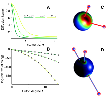
The diffusion process models many natural phenomena. Examples include heat diffusion and plume spreading from a smokestack. Often, the source of the diffusion process is localized in space, and instantaneous in time. Sampling such processes in Euclidean domains has been well studied [30, 31, 32].
Diffusion processes on the sphere are governed by the equation [33]
| (41) |
where is the Laplace-Beltrami operator on , and is the diffusion constant. In the spherical harmonic domain, this becomes
| (42) |
giving the solution
| (43) |
where is the spectrum of the initial distribution. Therefore, we interpret the term as the spectrum of the Green’s function of the spherical diffusion equation. In other words, it is the spectrum of the diffusion kernel on the sphere. Then (43) should be interpreted as the convolution between the kernel and the initial distribution.
We consider the case when the diffusion process is initiated by sources localized in space and time, i.e., the initial distribution in (43) is
| (44) |
We show how to use the proposed sampling algorithm to estimate the locations and the strengths of the sources from spatial samples of the diffusion field taken at a later time . Recovering all parameters (locations, amplitudes and release times) of multiple diffusion sources is a challenging task [30]. To focus on the proposed sampling result, we make the simplifying assumption that the sources are released simultaneously, and at a known time (). In principle, the more challenging case of unknown and different release times can be handled by adapting the techniques derived in [31, 32], but these generalizations are out of the scope of this work.
In the spatial domain, the diffusion kernel at time after the release is given as
| (45) |
Combining (45) with (43) and the spherical convolution-multiplication rule (13), we get
| (46) | ||||
This signal is a sum of rotations of a known template. The diffusion kernel in (45) is not exactly bandlimited, but it is approximately so. We can therefore apply the spherical FRI theory and Algorithm 1 to recover the locations and the magnitudes of the diffusive sources.
IV-B Shot Noise Removal
Suppose that we sample a bandlimited function on the sphere, but a small number of samples are corrupted—they contain shot noise—due to sensor malfunction. Moreover, the identities of the malfunctioning sensors are not known a priori. Can we detect and correct these anomalous measurements? We show that our sampling results can be applied to solve this problem, provided that the number of erroneous sensors is not too large and that the original sampling grid is oversampling the bandlimited function. A similar idea was used in [34] to remove shot noise in the 1D Euclidean case.
For this application we assume that the samples are taken on a uniform grid on the sphere, , defined by
| (48) |
Imagine now that we sample on this sampling grid. Some samples are corrupted, so we measure , where
| (49) |
and holds the indices of the corrupted samples. We will leverage an elegant quadrature rule by Driscoll and Healy [9]:
Theorem 2.
In other words, the Fourier coefficients can be expressed as a dot-product between weighted sample values and the basis functions evaluated at the sampling points. In analogy with the Euclidean case, we now observe that the lowpass portion of the spectrum of coincides with the lowpass portion of the spectrum of the generalized function obtained by placing weighted Diracs at grid points. Let be bandlimited so that for . Let further ; that is, the grid (48) oversamples . Then the spectral coefficients can be expressed as the following inner product,
| (51) |
for , .
This is the key insight. Notice that the lowpass portion of the spectrum of (for ) can be written as
| (52) |
But for , so the portion of the spectrum for contains only the influence of the corrupted samples,
| (53) |
Consequently, we can use this part of the spectrum to learn which samples are corrupted, and by how much. This is the subject of the following proposition.
Proposition 2.
Let be a signal on the sphere of bandwidth . Then we can perfectly reconstruct from corrupted samples taken on the grid (48), as long as the number of corruptions satisfies
| (54) |
Proof.
As discussed in Section III, we can use any line in the spectrum to get the rows of the annihilation matrix. However, we first need to compute the corresponding columns of the data matrix. From Fig. 5, we see that the middle columns cannot be used for shot noise removal: we seek columns influenced only by corruptions. But the middle columns of the data matrix are obtained from the middle spectral columns (for ), so they are influenced both by the desired signal and the corruptions. This means that we can only use spectral bins for , as illustrated in Fig. 5. For and , the number of segments of length that we can get is . For and it is , and so on. Summing up we have that the total number of consecutive segments of length we can use is
We need this number to be at least , because we need rows in the annihilation matrix. We thus obtain the claim of the proposition by solving the inequality . ∎


After detecting the corrupted readings, we can use the estimated corruption values to estimate the function. Another option is to simply ignore them altogether, as we have more samples than the minimum number thanks to oversampling. A shot noise removal experiment is illustrated in Fig. 6.
IV-C Sound Source Localization
Spherical microphone arrays output a time-varying spherical signal. If the signal is induced by a collection of point sources, we can use the proposed spherical FRI sampling scheme to estimate the directions-of-arrival (DOAs) of the sources. For simplicity, we consider the narrowband case, i.e., the sources emit a single sinusoid.
How does this example fit into our sparse sampling framework? In spherical microphone arrays, the microphones are distributed on the surface of a sphere, either open or rigid [7]. Therefore, the microphone signals represent samples of a time-varying function on . If a sound source emits a sinusoid, every microphone measures the amplitude and the phase of that sinusoid shaped by the characteristics of the propagating medium and of the spherical casing. Equivalently, for every microphone we get a complex number.
Suppose that a source of unit intensity is located at , and that the microphones are mounted on a rigid sphere of radius with center at the origin. The response measured by the microphone at , such that , is given by the corresponding Green’s function. For a wavenumber , where is the frequency and is the speed of sound, the Green’s function is [7]
| (55) |
where is the spherical Hankel function of the first kind and of order , is the Legendre polynomial, and . Mode strength is defined as
| (56) |
where is the spherical Bessel function33 3 We use the standard symbol for the spherical Bessel function. Note the subtle difference from the imaginary unit . of order , and prime denotes the derivative with respect to the argument.
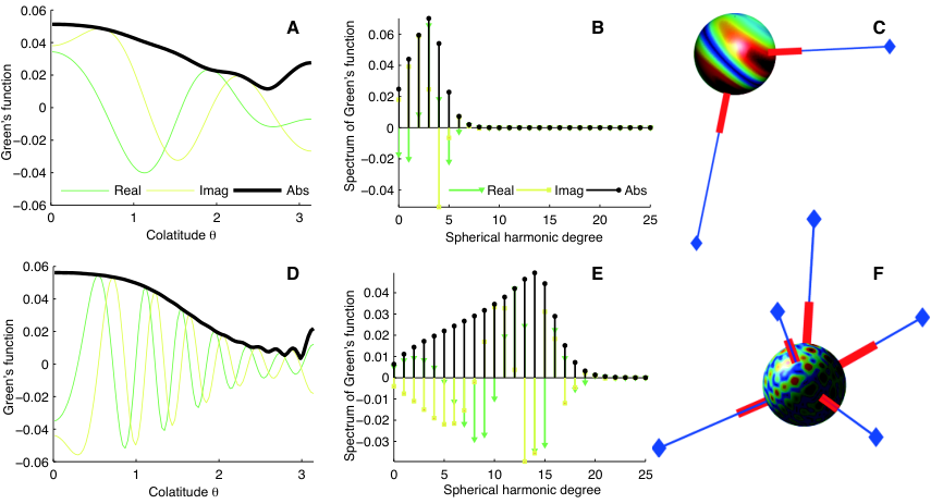
The Green’s function should be seen as a filter that describes how the point source’s influence spreads over the sphere. It is shown for two different frequencies in Figs. 7A and 7D, while the corresponding spectra are given in Figs. 7B and 7E. We see that the absolute pressure on the sphere has a similar shape for both frequencies, but the real and imaginary parts vary faster at higher frequencies, implying higher bandwidth. In both cases we observe that the Green’s function is approximately bandlimited.
Assume now that there are sound sources at locations , with complex intensities . The resulting measurement by a microphone at point is
| (57) |
If all the source locations are at the same distance from the sphere, then the Green’s function (55) depends only on the angle between and . For some fixed source distance , we can define , where denotes the unit vector corresponding to , the unit vector corresponding to the north pole , and the subscript SSL stands for sound source localization. Then (57) corresponds to a weighted sum of rotations of a known template function ,
| (58) |

As it is unrealistic to assume that the sources are all at the same distance, we hope that the shape of does not (strongly) depend on . Indeed, it turns out that the shape is approximately preserved within a certain range, as illustrated in Fig. 8. We therefore suppress the dependency of on and approximate (57) as follows,
| (59) | ||||
Here, we absorbed and additional (complex) scaling due to different distances into , and is computed at some predefined mean distance.
We thus reduced the sound source localization problem to a problem of finding the parameters of a weighted sum of Diracs. In order to apply our spherical FRI algorithm, we need to verify that is bandlimited on the sphere. Figs. 7D and 7E show that it is indeed approximately bandlimited, and that the bandwidth depends on the frequency (it also depends on the sphere radius).
Figs. 7C and 7D show an example of recovering two sources at 1000 Hz and 5 sources at 4000 Hz using the proposed spherical sparse sampling scheme. It is worth noting that this succeeds in spite of the model mismatch due to varying source distances. This indicates the robustness of the proposed reconstruction algorithm.
V Conclusion
We presented a new sampling theorem for sparse signals on the sphere. In particular, by leveraging ideas from finite rate-of-innovation sampling, we showed how to reconstruct sparse collections of spikes on the sphere from their lowpass-filtered observations. Compared to existing sparse sampling schemes on the sphere, we use the available spectrum more efficiently by generalizing known results on 2D harmonic retrieval, thereby reducing the number of samples required to reconstruct the parameters of the spikes.
We illustrated the usefulness of our algorithm by using it to solve three problems: sampling diffusion processes, shot noise removal, and sound source localization. But there is a wealth of other applications, for example in astronomy. Just think about the numerous spherical signal processing challenges put forward by the square kilometer array (SKA) project [35].
We mentioned some approaches to estimation from noisy samples, but more efficient denoising schemes should be studied. One example, effective in the Euclidean setting, is the Cadzow denoising algorithm [36]. The problem seems more challenging on the sphere; in particular, the annihilating matrix is block-Hankel, rather than Hankel.
-A Annihilating Property
For the sake of completeness, we show in this appendix that the annihilation filter annihilates linear combinations of exponentials. We compute the response of the filter in (33) to a signal of the form as
-B Computation of the Cramér-Rao Lower Bound
A lowpassed collection of Diracs can be written as follows,
| (60) |
In the remainder of this section, we assume , so we rewrite the function as
| (61) |
We take samples on the sphere at the locations . The th sample is given by
| (62) |
where , and they are iid. By , we denote the vector of parameters we estimate. To make the dependence on explicit, we rewrite (62) slightly as
| (63) |
With this notation in hand, we can write the conditional probability density function of the th measurement as
| (64) |
so that the log-likelihood function is
| (65) |
Consequently, differentiating with respect to any entry of gives
| (66) |
We can compute the three required derivatives
Now , and the Fisher information matrix is
Let be any unbiased estimator of the parameters . The CRLB can then be computed as
| (67) |
-C Rank of the annihilating matrix
In this appendix, we show that the rank of the annihilating matrix (35) is with probability one, as soon as it has at least rows. It then follows follows that the annihilating filter is uniquely determined, up to a scaling factor, by solving .
Consider the factorization ,
where and .
To construct the annihilating matrix as in equation (35), we create Hankel blocks from columns of . The Hankel block corresponding to the middle () column of can be factored as
| (68) |
The second block of the annihilating matrix obtained from the column corresponding to is similar,
| (69) |
where , and is obtained by removing the leading rows from . Then we can write
| (70) | ||||
with the factor being common for all row-blocks. We want to show that the nullspace of has dimension one. To that end, we just need to establish that the following matrix,
| (71) |
has full column rank. To see why this is the case, let be a non-zero vector such that . It then follows from the full-rankness of that . Since is a diagonal matrix with non-zero entries on the diagonal and is a Vandermonde matrix with distinct roots, the vector is uniquely determined up to a multiplicative factor. We now show that the matrix indeed has full column rank almost surely.
Any column in is of the form
| (72) |
where and . If the locations of the Diracs are random, we can use the following lemma to show that the matrix will have full column rank with probability one.
Lemma 3.
Draw independently at random from any absolutely continuous probability distribution on (w.r.t. Lebesgue measure). Let be a set of distinct integer pairs and let , where . Then has full rank almost surely.
Proof.
This proof is parallel to that of Theorem 3.2 from [28]. Let be the upper left minor of . We define the bad set as the set on which is singular,
| (73) |
The goal is to show that , where is the Lebesgue measure on . We proceed by induction on ; for , we have that
which is non-zero almost surely, so the claim holds. Assume now that and that the bad set has measure zero. Let , i.e., is invertible. Because it is invertible, there exists a unique coefficient vector such that
| (74) |
where by we denote the first entries of the last column of . The bigger matrix will be singular if and only if the same linear combination is also consistent with its st row. In other words, is invertible if and only if is not in the set
For fixed , this is the set of zeros of a particular (generalized) trigonometric polynomial, thus it has measure zero. Note that the definition of makes sense only for , as otherwise is not invertible. Thus, the solution to (74) may not exist.
Consider now the following two sets:
and
The bad set must be a subset of the set . But we just showed that the set has measure zero; by the induction hypothesis, also has measure zero. Thus their union, too, has measure zero.
It follows that has measure zero. Finally, because the distributions of are absolutely continuous w.r.t. the Lebesgue measure, so is their product distribution. Hence the probability that lies in the zero-measure set is zero. ∎
To complete the argument, note that the matrix has the same form as the matrix in the statement of Lemma 3, with and . Thus, the columns of are independent with probability one, provided that its number of rows is at least .
Acknowledgement
We thank Martin Vetterli for his support and mentoring.
References
- [1] K. F. Evans, “The Spherical Harmonics Discrete Ordinate Method for Three-Dimensional Atmospheric Radiative Transfer,” J. Atmos. Sci., vol. 55, no. 3, pp. 429–446, 1998.
- [2] F. J. Simons, F. A. Dahlen, and M. A. Wieczorek, “Spatiospectral Concentration on a Sphere,” SIAM Rev., vol. 48, no. 3, pp. 504–536, 2006.
- [3] P. Audet, “Directional Wavelet Analysis on the Sphere: Application to Gravity and Topography of the Terrestrial Planets,” J. Geophys. Res., vol. 116, no. E1, pp. 1–16, 2011.
- [4] N. Jarosik, C. L. Bennett, J. Dunkley, B. Gold, M. R. Greason, M. Halpern, R. S. Hill, G. Hinshaw, A. Kogut, E. Komatsu, D. Larson, M. Limon, S. S. Meyer, M. R. Nolta, N. Odegard, L. Page, K. M. Smith, D. N. Spergel, G. S. Tucker, J. L. Weiland, E. Wollack, and E. L. Wright, “Seven-year Wilkinson Microwave Anisotropy Probe (WMAP) Observations: Sky Maps, Systematic Errors, and Basic Results,” Astrophys. J. Suppl. Ser., vol. 192, no. 2, pp. 1–15, Feb. 2011.
- [5] R. H. Macphie and E. H. Okongwu, “Spherical Harmonics and Earth-Rotation Synthesis in Radio Astronomy,” IEEE Trans. Antennas Propag., vol. 23, no. 3, pp. 386–391, 1975.
- [6] J. Meyer and G. Elko, “A Highly Scalable Spherical Microphone Array Based on an Orthonormal Decomposition of the Soundfield,” in Proc. IEEE ICASSP, Orlando, FL, USA, 2002, pp. 1781–1784, IEEE.
- [7] D. P. Jarrett, E. A. P. Habets, M. R. P. Thomas, and P. A. Naylor, “Rigid Sphere Room Impulse Response Simulation: Algorithm and Applications,” J. Acoust. Soc. Am., vol. 132, no. 3, pp. 1462–1472, 2012.
- [8] J. D. Tournier, F. Calamante, D. G. Gadian, and A. Connelly, “Direct Estimation of the Fiber Orientation Density Function from Diffusion-Weighted MRI Data Using Spherical Deconvolution,” NeuroImage, vol. 23, no. 3, pp. 1176–1185, Nov. 2004.
- [9] J. R. Driscoll and D. M. Healy, “Computing Fourier Transforms and Convolutions on the 2-Sphere,” Adv. Appl. Math., vol. 15, no. 2, pp. 202–250, June 1994.
- [10] J. D. McEwen and Y. Wiaux, “A Novel Sampling Theorem on the Sphere,” IEEE Trans. Signal Process., vol. 59, no. 12, pp. 5876–5887, 2011.
- [11] Z. Khalid, R. A. Kennedy, and J. D. McEwen, “An Optimal-Dimensionality Sampling Scheme on the Sphere With Fast Spherical Harmonic Transforms,” IEEE Trans. Signal Process., vol. 62, no. 17, pp. 4597–4610, 2014.
- [12] M. Vetterli, P. Marziliano, and T. Blu, “Sampling Signals with Finite Rate of Innovation,” IEEE Trans. Signal Process., vol. 50, no. 6, pp. 1417–1428, June 2002.
- [13] I. Maravic and M. Vetterli, “Exact Sampling Results for Some Classes of Parametric Nonbandlimited 2-D Signals,” IEEE Trans. Signal Process., vol. 52, no. 1, pp. 175–189, Jan. 2004.
- [14] P. Shukla and P. L. Dragotti, “Sampling Schemes for Multidimensional Signals With Finite Rate of Innovation,” IEEE Trans. Signal Process., vol. 55, no. 7, pp. 3670–3686, 2007.
- [15] I. Maravic and M. Vetterli, “Sampling and Reconstruction of Signals With Finite Rate of Innovation in the Presence of Noise ,” IEEE Trans. Signal Process., vol. 53, no. 8, pp. 2788–2805, Aug. 2005.
- [16] P. L. Dragotti and F. Homann, “Sampling Signals with Finite Rate of Innovation in the Presence of Noise,” in Proc. IEEE ICASSP, Taipei, Taiwan, 2009, pp. 2941–2944, IEEE.
- [17] S. Deslauriers-Gauthier and P. Marziliano, “Sampling Signals With a Finite Rate of Innovation on the Sphere,” IEEE Trans. Signal Process., vol. 61, no. 18, pp. 4552–4561, 2013.
- [18] S. Deslauriers-Gauthier and P. Marziliano, “Sampling Great Circles at Their Rate of Innovation,” in Proc. SPIE Wavelets and Sparsity, D. Van De Ville, V. K. Goyal, and M. Papadakis, Eds., San Diego, CA, USA, Sept. 2013, International Society for Optics and Photonics.
- [19] S. Deslauriers-Gauthier and P. Marziliano, “Spherical Finite Rate of Innovation Theory for the Recovery of Fiber Orientations,” in Proc. IEEE EMBC, San Diego, CA, USA, 2012, pp. 2294–2297.
- [20] T. Bendory, S. Dekel, and A. Feuer, “Super-resolution on the Sphere using Convex Optimization,” arXiv, Dec. 2014.
- [21] T. Bendory, S. Dekel, and A. Feuer, “Exact Recovery of Dirac Ensembles from the Projection Onto Spaces of Spherical Harmonics,” Constr Approx, pp. 1–25, 2014.
- [22] E. J. Candès and C. Fernandez Granda, “Towards a Mathematical Theory of Super-resolution,” Communications on Pure and Applied Mathematics, vol. 67, no. 6, pp. 906–956, June 2014.
- [23] S. M. Kay, Fundamentals of Statistical Signal Processing: Estimation theory, 1998.
- [24] M. Abramowitz and I. A. Stegun, “Handbook of mathematical functions,” National Bureau of Standards, 1972.
- [25] D. A. Varshalovich, A. N. Moskalev, and V. K. Khersonskii, Quantum Theory of Angular Momentum, World Scientific, Singapore, 1989.
- [26] I. Dokmanić and D. Petrinović, “Convolution on the -Sphere With Application to PDF Modeling,” IEEE Trans. Signal Process., vol. 58, no. 3, pp. 1157–1170, Mar. 2010.
- [27] D. Duffy, Green’s Functions with Applications, Chapman and Hall/CRC, 2001.
- [28] R. F. Bass and K. Gröchenig, “Random Sampling of Multivariate Trigonometric Polynomials,” SIAM J. Math. Anal., vol. 36, no. 3, pp. 773–795, Jan. 2005.
- [29] F. Vanpoucke, M. Moonen, and Y. Berthoumieu, “An Efficient Subspace Algorithm for 2-D Harmonic Retrieval,” in Proc. IEEE ICASSP, Adelaide, SA, Australia, 1994, pp. 461–464, IEEE.
- [30] I. Dokmanić, J. Ranieri, A. Chebira, and M. Vetterli, “Sensor Networks for Diffusion Fields: Detection of Sources in Space and Time,” in Proc. Allerton, 2011, pp. 1552–1558.
- [31] Y. M. Lu and M. Vetterli, “Distributed spatio-temporal sampling of diffusion fields from sparse instantaneous sources,” in Proc. IEEE CAMSAP, Aruba, 2009.
- [32] Y. M. Lu, P. L. Dragotti, and M. Vetterli, “Localizing Point Sources in Diffusion Fields From Spatiotemporal Samples,” in Proc. SampTA, Signapore, 2011.
- [33] T. Bulow, “Spherical Diffusion for 3D Surface Smoothing,” IEEE Trans. Pattern Anal. Mach. Intell., vol. 26, no. 12, pp. 1650–1654, 2004.
- [34] P. Marziliano, M. Vetterli, and T. Blu, “Sampling and exact reconstruction of bandlimited signals with additive shot noise,” IEEE Trans. Inf. Theory, vol. 52, no. 5, pp. 2230–2233, May 2006.
- [35] P. E. Dewdney, P. J. Hall, R. T. Schilizzi, and T. J. L. W. Lazio, “The Square Kilometre Array,” Proc. IEEE, vol. 97, no. 8, pp. 1482–1496, June 2009.
- [36] J. A. Cadzow, “Signal Enhancement—A Composite Property Mapping Algorithm,” IEEE Trans. Acoust., Speech, Signal Process., vol. 36, no. 1, pp. 49–62, 1988.