Mechanical Design, Modelling and Control of a Novel Aerial Manipulator

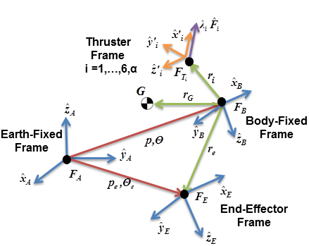
Initially, we define the Body-Fixed frame and the End-Effector frame as $F_{B}=\{\hat{x}_{B},\hat{y}_{B},\hat{z}_{B}\},F_{E}=\{\hat{x}_{E},\hat{y}_{E},\hat{z}_{E}\}$. These frames are attached to the rigid body of the aerial manipulator as in Fig. 1. The vectors $r_{i},r_{e}\in\mathbb{R}^{3}$ denote the position of each thruster and the position of the end-effector respectively with reference to the Body-Fixed frame. The thruster orientations are given by the unit vectors $\hat{F}_{i}\in\mathbb{R}^{3},\ i=1,...,n$, the thrust forces are defined as $\lambda_{i}$ and the propulsion vectors are given by $\lambda_{i}\ \hat{F}_{i}$. At this point, it is assumed that the total system is considered to be a rigid body and, without loss of generality, the End-Effector frame and the Body frame have the same orientation. Thus, the actuation force applied to the end-effector is $F_{act}\big\lvert_{B}=F_{act}\big\lvert_{E}\in\mathbb{R}^{3}$, where $\big\lvert_{B},\big\lvert_{E}$ denote the expressions to the frames $F_{B},F_{E}$ respectively. The corresponding actuation torque is obtained via the formula $T_{act}\big\lvert_{B}=T_{act}\big\lvert_{E}+r_{e}\times f_{e}$ where $T_{act}\big\lvert_{E}=r\times f_{e}$ is the torque produced by the end-effector. The terms $r,f_{e}$ denote the displacement vector (length of the lever arm) and the vector force that tends to rotate a gripped object from the end-effector.

The forces transmitted essentially through the end-effector are written as

$$\sum_{i=1}^{n}(\lambda_{i}\ \hat{F}_{i})+W=F_{act}\big\lvert_{B}$$

(1)

where $W\in\mathbb{R}^{3}$ is the vector that corresponds to the total weight of the system. By separating the weight as $w_{s}=W-n\ w$, where $w\in\mathbb{R}^{3}$ is the weight of each thruster, (1) is modified as

$$F\ \lambda+n\ w+w_{s}=F_{act}\big\lvert_{B}$$

(2)

where $\displaystyle\lambda=[\lambda_{1}\cdots\lambda_{n}]^{\tau}\in\mathbb{R}^{n}$ and $\displaystyle F=[\hat{F}_{1}\cdots\hat{F}_{n}]^{\tau}\in\mathbb{R}^{3\times n}$.

Similarly, the torque from each thruster is $T_{i}=r_{i}\times(\lambda_{i}\hat{F}_{i})=\lambda_{i}S(r_{i})\hat{F}_{i}$. The well-known skew-symmetric matrix $S(\cdot)\in\mathbb{R}^{3\times 3}$ is defined as $a\times b=S(a)\ b$ for the cross-product $\times$ and any vectors $a,b\ \in\mathbb{R}^{3}$. The torque due to the weight is calculated as

$$T_{W}=r_{G}\times W=\displaystyle\sum_{i=1}^{n}r_{i}\times w+r_{s}\times w_{s}=\displaystyle\sum_{i=1}^{n}S(r_{i})w+S(r_{s})w_{s}$$

where $r_{G}$ is the centre of gravity of the system and $r_{s}$ is the centre of gravity of the system, when omitting the mass of each thruster ($m_{\text{thr}}$). The reaction torque of each thruster is $\tau_{i}=\mu\ (\lambda\ \hat{F}_{i})$ where $\mu$ is a coefficient that represents the relationship between the thrust force and the reaction torque [15]. Therefore, by combining all torques the following equation holds

$$\sum_{i=1}^{n}\left\{\lambda_{i}\ S(r_{i})\ \hat{F}_{i}\right\}+\mu\ \sum_{i=1}^{n}\left(\lambda_{i}\ \hat{F}_{i}\right)\\ +\sum_{i=1}^{n}S(r_{i})\ w+S(r_{s})\ w_{s}=T_{act}\big\lvert_{B}$$

(3)

Using the matrices

		$\displaystyle r=\begin{bmatrix}r_{1}&\cdots&r_{n}\end{bmatrix}^{\tau}\in\mathbb{R}^{3\times n},\bar{F}=F_{act}\big\lvert_{B}-n\ w-w_{s}$		(4)
		$\displaystyle E(r,F)=\begin{bmatrix}S(r_{1})\ \hat{F}_{1}&\cdots&S(r_{n})\ \hat{F}_{n}\end{bmatrix}\in\mathbb{R}^{3\times n}$		(5)

in (2),(3) we get

$$\begin{cases}F\ \lambda=\bar{F}\\ E\ \lambda=T_{act}\big\lvert_{B}-\mu\ \bar{F}-\displaystyle\sum_{i=1}^{n}S(r_{i})\ w-S(r_{s})\ w_{s}\\ \end{cases}$$

(6)

By defining the matrix $D(r,F)=\begin{bmatrix}F\\ E(r,F)\\ \end{bmatrix}\in\mathbb{R}^{6\times n}$, from the system (6) it is implied that

$$D(r,F)\ \lambda=W_{R}$$

(7)

where the augmented wrench vector $W_{R}\in\mathbb{R}^{6}$ is given by

$$W_{R}=\begin{bmatrix}\bar{F}\\ T_{act}\big\lvert_{B}-\mu\bar{F}-\displaystyle\sum_{i=1}^{n}S(r_{i})w-S(r_{s})w_{s}\\ \end{bmatrix}$$

(8)

It is clear that when solving (7), the vector that corresponds to the thrust force $\lambda$ can obtain any value in $\mathbb{R}^{6}$. However, the thrusters are optimally designed to produce thrust force towards a specific direction, which we set to correspond to the positive values of $\lambda_{i}$. In order to alleviate the problem of negative $\lambda_{i}$, a conservative solution is adopted in this analysis, which is based on the idea of introducing one additional thruster. Thus, (7) is rewritten as

$$\sum_{i=1}^{n}\lambda_{i}\ t_{i}=W_{R}$$

(9)

where

$$D(r,F)=\displaystyle[t_{1}\ t_{2}\ \cdots\ t_{n}]\ \text{and}\ t_{i}=\begin{bmatrix}\hat{F}_{i}\\ S(r_{i})\ \hat{F}_{i}\\ \end{bmatrix}\in\mathbb{R}^{6}$$

(10)

for all $i=1,...,n$. The vector

$$t_{a}=-\sum\limits_{i=1}^{n}t_{i}=\begin{bmatrix}-\sum\limits_{i=1}^{n}\hat{F}_{i}\\[8.00003pt] -\sum\limits_{i=1}^{n}\left\{S(r_{i})\hat{F}_{i}\right\}\end{bmatrix}=\begin{bmatrix}\hat{F}_{a}\\ S(r_{a})\hat{F}_{a}\\ \end{bmatrix}$$

(11)

that corresponds to the additional thruster is introduced. Using (11), the position vector $r_{a}$ and the direction $\hat{F}_{a}$ of the new thruster should satisfy the equations $\hat{F}_{a}=-\sum\limits_{i=1}^{n}\hat{F}_{i}\ ,\ S(\hat{F}_{a})\ r_{a}=-\sum\limits_{i=1}^{n}\left\{S(\hat{F}_{i})\ r_{i}\right\}$.

If we assume that (7) results in some negative thrust forces, then the set $\sigma_{N}=\left\{k:\lambda_{k}<0,k=1,...,6\right\}$ denotes the indexes for every negative thrust force and $\sigma_{P}=\left\{1,2,3,4,5,6\right\}-\sigma_{N}$ the corresponding set of positive thrust forces. Observing that $\lambda_{k}<0\Leftrightarrow(-\lambda_{k})>0,\ \forall\ k\in\sigma_{N}$, (9) can be separated in

	$\displaystyle\sum_{i\in\sigma_{P}}\lambda_{i}\ t_{i}+\sum_{k\in\sigma_{N}}\lambda_{k}\ t_{k}$	$\displaystyle=W_{R}$
	$\displaystyle\Leftrightarrow\sum_{i\in\sigma_{P}}\lambda_{i}\ t_{i}+\sum_{k\in\sigma_{N}}(-\lambda_{k})\ (-t_{k})$	$\displaystyle=W_{R}$		(12)

Now, from (11) the following can be exported

$$t_{a}=-\sum\limits_{i=1}^{n}t_{i}=-\sum_{i\in\sigma_{P}}t_{i}-\sum_{j\in\sigma_{N}}t_{j}$$

(13)

It is obvious that

$$-\sum_{j\in\sigma_{N}}t_{j}=-t_{k}-\sum_{\begin{subarray}{c}j\in\sigma_{N}\\ j\neq k\end{subarray}}t_{j},\ \forall\ k\in\sigma_{N}$$

(14)

Combining (13), (14) we obtain

$$-t_{k}=t_{a}+\sum_{i\in\sigma_{P}}t_{i}+\sum_{\begin{subarray}{c}j\in\sigma_{N}\\ j\neq k\end{subarray}}t_{j},\ \forall\ k\in\sigma_{N}$$

(15)

By substituting (15) into (12) we have

$\displaystyle\sum_{i\in\sigma_{P}}\lambda_{i}\ t_{i}+\sum_{k\in\sigma_{N}}(-\lambda_{k})\bigg[t_{a}+\sum_{i\in\sigma_{P}}t_{i}+\sum_{\begin{subarray}{c}j\in\sigma_{N}\\ j\neq k\end{subarray}}t_{j}\bigg]=W_{R}$

Defining

$$\Delta=\sum_{k\in\sigma_{N}}(-\lambda_{k})>0,\ E_{k}=\sum_{\begin{subarray}{c}j\in\sigma_{N}\\ j\neq k\end{subarray}}(-\lambda_{j})>0$$

(16)

and rearranging the terms we result in

$$\sum_{i\in\sigma_{P}}\big(\lambda_{i}+\Delta\big)t_{i}+\sum_{k\in\sigma_{N}}E_{k}\ t_{k}+\Delta\ t_{a}=W_{R}$$

(17)

From (17) the thruster redistribution among all thrusters after adding the new thruster is provided. It has been proven that the issue of negative thrust forces can be alleviated with adding one extra thruster. This equation can be better analysed in Fig. 2 in which the thrust redistribution algorithm is depicted. The variables $\lambda^{\prime},\lambda_{i}^{\prime},\lambda_{k}^{\prime}$ denote the initial thrust forces and the other variables the thrust force after the redistribution, plus the additional thrust force $\lambda_{a}$. Thus, the six thrust forces (not necessary all positive) are equivalent to seven thrust forces, all positive with redistributed thrust forces as in (17). By using the additional thruster, (4), (8) are reformed into

	$\displaystyle\bar{F}$	$\displaystyle=F_{act}\big\lvert_{B}-(n+1)\ w-w_{s}$		(18)
	$\displaystyle W_{R}$	$\displaystyle=\begin{bmatrix}\bar{F}\\ T_{act}\big\lvert_{B}-\mu\ \bar{F}-\displaystyle\sum_{i=1}^{n+1}S(r_{i})\ w-S(r_{s})\ w_{s}\\ \end{bmatrix}$		(19)

At this point, the aerodynamic interaction between the operation thrusters is investigated. The aerodynamic effects produced by each thruster, are based on experiments that took place in Control Systems Lab NTUA on a $8\times 4.7SF$ APC propeller accompanied with the Neu Motor NEU 1902/2Y - 2035 motor, which produces at 17550 rpm, a $\lambda_{\text{max}}=28N$ thrust force. The surface, corresponding to every thruster, that approximates these effects is described by a third order equation in (SI). By expressing this equation in the thruster frame $F_{T_{i}}=\{\hat{x}^{\prime}_{i},\hat{y}^{\prime}_{i},\hat{z}^{\prime}_{i}\},i=1,...,6,a$ we get

	$\displaystyle-0.06$	$\displaystyle\leq x^{\prime}_{i}\leq 0.91$		(20)
	$\displaystyle(y^{\prime}_{i})^{2}+(z^{\prime}_{i})^{2}$	$\displaystyle\leq\left[-1.1(x^{\prime}_{i})^{3}+1.56(x^{\prime}_{i})^{2}-0.3(x^{\prime}_{i})+0.11\right]^{2}$

Hence, the aerodynamic effects of the air flow throughout the rotor are extended from $x=-0.06m$ to $x=0.91m$. The $x$ axis shows the length of the aerodynamic effect of the exit flow. In order to understand this, one should consider the rotor/blade to be positioned at $x=0$. On the other hand, $y$ axis shows the distance of the effect measured from the rotation axis of the blade, where at position $(x=0,y=0.102m)$ (SI) is the blade radius in approximation (because of the existence of an offset).

An arbitrary point $p=\left[x\ y\ z\right]^{\tau}$ expressed in $F_{B}$ and the corresponding $p^{\prime}_{i}=\left[x^{\prime}_{i}\ y^{\prime}_{i}\ z^{\prime}_{i}\right]^{\tau}$ expressed in $F_{T_{i}}$, can be linked together by the equation $p=\{TR_{F_{B}}^{F_{T_{i}}}(r_{i},\hat{F}_{i})\}\ p^{\prime}_{i}$, where $TR_{F_{B}}^{F_{T_{i}}}(r_{i},\hat{F}_{i})$ is the appropriate homogeneous frame transformation corresponding to the translation and orientation vectors $(r_{i},\hat{F}_{i})$. By combining the previous coordinates transformation equation with the constraints (20), a set of constraints that can be described in matrix form as $G(r_{i},\hat{F}_{i},p)\leq 0$, is produced. The distance between two such volumes $i$, $j$ can be defined and evaluated via the optimization problem $(P_{1})$ of Table I.

Given a particular structure defined by the matrices $(r,F)$, for a set of required actuation forces and torques $(F_{act}\big\lvert_{E},T_{act}\big\lvert_{E})$ it is necessary to find the associate levels of the thrust forces $\lambda_{i}$. Since $W_{R}\in\mathbb{R}^{6}$, in order for (7) to have a solution for $\lambda\in\mathbb{R}^{n}$, the conditions $\{\text{rank}(D)=6,n\geq 6\}$ are required. The rank condition is adequate from a strict mathematical perspective but from a practical point of view, as (7) leads to the thrust forces values $\lambda\in\mathbb{R}^{n}$, the sought solutions should not be very sensitive to small deviations. This is partially achieved by using the condition number $\kappa(D)=\sigma_{\text{max}}(D)/\sigma_{\text{min}}(D)$ where $\sigma(D)=\sqrt{\text{eig}(\displaystyle D^{\tau}D)}$ are the singular values of the matrix D, $\text{eig}(\cdot)$ denotes the eigenvalues of a matrix and $\sigma_{\text{max}}(D),\sigma_{\text{min}}(D)$ are the maximum and minimum singular values of the matrix $D$ respectively. Thus, a low condition number $\kappa(D)\geq 1$ is required [16]. Although the condition number is bounded to take feasible values (not equal to zero/infinity) when $\sigma(D)\rightarrow 0$, the matrix $D(r,F)$ might be ill-conditioned i.e. $\text{det}(D(r,F))\rightarrow 0$. Thus, $\sigma(D)\geq\epsilon_{1}>0$. Furthermore, to avoid the fan interaction an other constraint is introduced as $d_{ij}(r_{i},\hat{F}_{i},r_{j},\hat{F}_{j})\geq\epsilon_{2}>0,\ \forall i,j=1,2,\dots,n,\alpha$. Note that, similarly to $(P_{1})$, the position $r_{e}$ should be introduced to the design problem as the intersection avoidance between a sphere (with radius $R_{e}$) that encloses the end-effector, and the thrusters. This sphere, when expressed in the End-Effector frame $F_{E}$, is given by $(x^{\prime}_{e})^{2}+(y^{\prime}_{e})^{2}+(z^{\prime}_{e})^{2}\leq R_{e}^{2}$. Therefore, the constraint associated with the end-effector is $d_{ei}(r_{e},r_{i})\geq R_{e}>0,\ \forall i=1,2,\dots,n,\alpha$. An optimization is also required to minimize the volume of the system, by using the norm $J(r)=\|r\|_{2}$. Taking all the above into consideration, the design problem is essentially recast to the optimization problem $(P_{2})$ from Table I. The optimization parameters are chosen as $K=5,\ \epsilon_{1}=10^{-3},\ \epsilon_{2}=10^{-2}\ m,\ R_{e}=10^{-2}\ m$.

It should be noted that when solving the optimization problem $(P_{2})$, each time the inner problem $(P_{1})$ should be solved. There are 45 decision variables of the optimization problem, which correspond to the seven position vectors ($r_{i}$) of the thrusters, the position vector ($r_{e}$) of the end-effector and the direction vectors ($\hat{F}_{i}$) of the seven thrusters. This issue, entails the necessity of solving 28 optimization problems for each evaluation attempt of the outer problem $(P_{2})$.

The inner problem, that refers to the avoidance of the fan interaction, is smooth but in terms of the outer problem $(P_{2})$ is nonsmooth and nonlinear. The objective function and the constraints of the problem $(P1)$ are continuous and this problem, according to the inputs, has one and only one global minimum. Using the appropriate rotation and transformation matrices, the $(P1)$ was solved by the active-set strategy [17],[18]. On the other hand, the design problem $(P_{2})$ has nonsmooth, discontinuous and nonlinear inequality constraints, but smooth objective function. Consequently, a non-gradient-based methodology that searches disjoint feasible regions, is utilized. For the pre-search of the design space, a Latin Hypercube (LHS) [19] was chosen, in order to ensure that the points are distributed throughout the search space. The Latin Hypercube sampling is known to provide better coverage than the simple random sampling [20]. Following this, a Generalized Pattern Search (GPS) direct search algorithm [21],[22] was used.

The thrust force ($\lambda$) and the momentum (Q) can be calculated from [23],[24] as

$$\begin{cases}Q=\pi\rho\ C_{Q}\ R^{5}\ \Omega^{2}\\ \lambda=\pi\rho\ C_{\lambda}\ R^{4}\ \Omega^{2}\\ \end{cases}\Leftrightarrow\ \ Q=\frac{C_{Q}}{C_{\lambda}}\ R\ \lambda$$

(21)

where the term $\frac{C_{Q}}{C_{\lambda}}\ R$ corresponds to the coefficient $\mu$, $R$ is the radius of the rotor and $\rho,\Omega$ denote the air density and the rotational speed of the rotor respectively. Applying a combination of the Blade Element Theory [24] and the Momentum Theory [15], using the modified versions proposed in [23] and invoking the experimental results extracted by our lab on the APC propeller, it was calculated that $C_{\lambda}=0.008,C_{Q}=0.0095,\mu=0.1473,R=0.124m$. By solving the optimization problems, with the results depicted in Table II, the matrix $D(r,F)$ is full rank and using (7), the thrust forces can be calculated as $\lambda=D^{-1}\ W_{R}$. All the constraints were satisfied and a low volume body structure with condition number $\kappa(D)=3.36$ resulted. The wrench vector $W_{R}$ can be determined by substituting the desired actuation forces/torques ($F_{act}\big\lvert_{E}$, $T_{act}\big\lvert_{E}$) in (19). The maximum thrust force and torque which can be applied from the system are $\lambda_{\text{max}}=28N$ and $3Nm$ respectively. The values of the components, proposed for the Aerial Manipulator, are the following: the motor and the propeller $(0.12kg)$, the frame $(0.66kg)$, the battery $(0.25kg)$ and the electronic components $(0.15kg)$. The total mass of the proposed system is $m=1.90kg$. Ultimately, the production of a carefully studied framework (Fig. 3) was achieved by using the 3D CAD Package SolidWorks. Using this Package, the system parameter values of the Table II have been evaluated.

Fig. 1 shows the reference frames defined to derive the kinematic and dynamic model of the proposed system. The Earth-Fixed inertial frame is defined as $F_{A}=\{\hat{x}_{A},\hat{y}_{A},\hat{z}_{A}\}$ and it should be noted that the Body-Fixed frame’s origin does not coincide with the centre of gravity $G$. The position of $F_{B}$ relative to $F_{A}$ can be represented by $p=\left[x\ y\ z\right]^{\tau}\in\mathbb{R}^{3}$ and the corresponding orientation by the rotation angles $\Theta=\left[\phi\ \theta\ \psi\right]^{\tau}\in\mathbb{R}^{3}$. The translational and rotational kinematic equations of the moving rigid body are given (see [25]) in matrix form by

$$\dot{\xi}=\begin{bmatrix}\dot{p}\\ \dot{\Theta}\\ \end{bmatrix}=\begin{bmatrix}J_{t}(\Theta)&O_{(3\times 3)}\\ O_{(3\times 3)}&J_{r}(\Theta)\\ \end{bmatrix}\begin{bmatrix}v\\ \omega\\ \end{bmatrix}\\$$

(22)

where $O_{(3\times 3)}$ is the $3\times 3$ zero matrix, $v=\left[v_{x}\ v_{y}\ v_{z}\right]^{\tau}\in\mathbb{R}^{3},\ \omega=\left[\omega_{x}\ \omega_{y}\ \omega_{z}\right]^{\tau}\in\mathbb{R}^{3}$ denote the translational velocity and the angular velocity of $F_{B}$ relative to $F_{A}$ respectively, both expressed in the Body-Fixed frame. The transformation matrices $J_{t}(\Theta),J_{r}(\Theta)\in\mathbb{R}^{3\times 3}$ are given by

$$J_{t}(\Theta)=\begin{bmatrix}c_{\theta}c_{\psi}&s_{\phi}s_{\theta}c_{\psi}-s_{\psi}c_{\phi}&s_{\theta}c_{\phi}c_{\psi}+s_{\phi}s_{\psi}\\ s_{\psi}c_{\theta}&s_{\phi}s_{\theta}s_{\psi}+c_{\phi}c_{\psi}&s_{\theta}s_{\psi}c_{\phi}-s_{\phi}c_{\psi}\\ -s_{\theta}&s_{\phi}c_{\theta}&c_{\phi}c_{\theta}\\ \end{bmatrix}$$

(23)

$$J_{r}(\Theta)=\begin{bmatrix}1&s_{\phi}t_{\theta}&c_{\phi}t_{\theta}\\ 0&c_{\phi}&-s_{\phi}\\ 0&s_{\phi}/c_{\theta}&c_{\phi}/c_{\theta}\\ \end{bmatrix}$$

(24)

The position of the end-effector with respect to $F_{A}$ is $p_{e}=\left[x_{e}\ y_{e}\ z_{e}\right]^{\tau}=p+J_{t}(\Theta)\ r_{e}\in\mathbb{R}^{3}$. Its derivative is obtained as $\dot{p}_{e}=J_{t}(\Theta)\ v-J_{t}(\Theta)\ S(r_{e})\ \omega$, using the formula $\dot{J}_{t}(\Theta)=J_{t}(\Theta)S(\omega)$ from [26]. The Body-Fixed and the End-Effector frame have the same orientation with reference to $F_{A}$, as mentioned in Section II, hence $\Theta_{e}=\Theta$. By combining the last results the following kinematic equation holds

$$\dot{\xi}_{e}=\begin{bmatrix}\dot{p}_{e}\\ \dot{\Theta}\\ \end{bmatrix}=\underbrace{\begin{bmatrix}J_{t}(\Theta)&-J_{t}(\Theta)\ S(r_{e})\\ O_{(3\times 3)}&J_{r}(\Theta)\\ \end{bmatrix}\\ }_{\begin{subarray}{c}J(\xi_{e})\end{subarray}}\begin{bmatrix}v\\ \omega\\ \end{bmatrix}\\$$

(25)

where $\Theta_{e}$ is the orientation of $F_{E}$ relative to $F_{A}$. The Jacobian matrix of the system $J(\xi_{e})\in\mathbb{R}^{6\times 6}$ relates in a straightforward way the linear velocity $\dot{p}_{e}$ and the rate of change in the rotational angles $\dot{\Theta}$ of the end-effector expressed in $F_{A}$, with the Body-Fixed velocities $v,\omega$.

The dynamic equations can be conveniently written with respect to the Body-Fixed frame by using the Newton-Euler formalism (the main concept is discussed extensively in [27, 28]), as

$$M\ \begin{bmatrix}\dot{v}\\ \dot{\omega}\\ \end{bmatrix}+C(\nu)\ \begin{bmatrix}v\\ \omega\\ \end{bmatrix}=\begin{bmatrix}F\big\lvert_{B}\\ T\big\lvert_{B}\\ \end{bmatrix}$$

(26)

where

$$M=\begin{bmatrix}mI_{3}&-mS(r_{G})\\ mS(r_{G})&I_{B}\\ \end{bmatrix},\ M>0,\ \dot{M}=0$$

(27)

is the inertia matrix,

$$C=\begin{bmatrix}mS(\omega)&-mS(\omega)S(r_{G})\\ mS(r_{G})S(\omega)&-S(I_{B}\omega)\\ \end{bmatrix},C=-C^{\tau}$$

(28)

is the Coriolis-centripetal matrix, $I_{3}$ is the $3\times 3$ identity matrix, $m$ is the total mass of the system, $I_{B}$ is the inertia tensor expressed in $F_{B}$ and $\nu=\left[v^{\tau}\ \omega^{\tau}\right]^{\tau}\in\mathbb{R}^{6}$ is the vector of the Body-Fixed velocities. The inertia tensor can be written as $I_{B}=I_{G}-mS(r_{G})S(r_{G})$ where $I_{G}$ is the inertia tensor relative to the body’s centre of gravity. The vectors $F\big\lvert_{B},T\big\lvert_{B}\in\mathbb{R}^{3}$ describe the forces and torques acting on the system expressed in the Body-Fixed frame and can be derived as

	$\displaystyle\begin{bmatrix}F\big\lvert_{B}\\ T\big\lvert_{B}\\ \end{bmatrix}$	$\displaystyle=\begin{bmatrix}F\ \lambda-m\ g\ J^{\tau}_{t}(\Theta)\ e_{3}\\ E\ \lambda+\mu\ F\ \lambda-m\ g\ S(r_{G})\ J^{\tau}_{t}(\Theta)\ e_{3}\\ \end{bmatrix}$
		$\displaystyle=\underbrace{\begin{bmatrix}F\\ E\\ \end{bmatrix}\lambda}_{\text{propulsion}\atop\text{forces/torques}}+\underbrace{\begin{bmatrix}O_{(3\times 6)}\\ \mu\ F\\ \end{bmatrix}\lambda}_{\text{reaction}\atop\text{torques}}-\underbrace{m\ g\begin{bmatrix}I_{3}\\ S(r_{G})\\ \end{bmatrix}J_{t}^{\tau}(\Theta)e_{3}}_{\text{gravitational}\atop\text{forces/torques}}$		(29)

where $e_{3}=\left[0\ 0\ 1\right]^{\tau}$. Combining (26), (29) and solving with respect to $\left[\dot{v}^{\tau}\ \dot{\omega}^{\tau}\right]^{\tau}$ we get

	$\displaystyle\begin{bmatrix}\dot{v}\\ \dot{\omega}\\ \end{bmatrix}$	$\displaystyle=-M^{-1}C(\nu)\begin{bmatrix}v\\ \omega\\ \end{bmatrix}+M^{-1}\ \begin{bmatrix}F\\ E+\mu\ F\\ \end{bmatrix}\lambda$
		$\displaystyle\qquad{}-m\ g\ M^{-1}\ \begin{bmatrix}I_{3}\\ S(r_{G})\\ \end{bmatrix}J_{t}^{\tau}(\Theta)\ e_{3}$		(30)
	$\displaystyle\Leftrightarrow\dot{\nu}$	$\displaystyle=\underbrace{H(\nu)+G(\xi_{e})}_{B(\xi_{e},\nu)}+N\ \lambda$		(31)

where the matrices are defined as

		$\displaystyle H(\nu)=-M^{-1}\ C(\nu)\ \nu,N=M^{-1}\ \begin{bmatrix}F\\ E+\mu\ F\\ \end{bmatrix}>0$		(32)
		$\displaystyle G(\xi_{e})=-m\ g\ M^{-1}\ \begin{bmatrix}I_{3}\\ S(r_{G})\\ \end{bmatrix}J_{t}^{\tau}(\Theta)e_{3}$		(33)
		$\displaystyle B(\xi_{e},\nu)=H(\nu)+G(\xi_{e}),\ B:\mathbb{R}^{6}\times\mathbb{R}^{6}\rightarrow\mathbb{R}^{6}$		(34)

References

- [1] L. Marconi, R. Naldi, and L. Gentili, “Modelling and Control of a Flying Robot Interacting with the Environment,” Automatica, vol. 47, no. 12, pp. 2571–2583, 2011.
- [2] A. Keemink, M. Fumagalli, S. Stramigioli, and R. Carloni, “Mechanical Design of a Manipulation System for Unmanned Aerial Vehicles,” IEEE International Conference on Robotics and Automation (ICRA), pp. 3147–3152, 2012.
- [3] A. Albers, S. Trautmann, T. Howard, T. Nguyen, M. Frietsch, and C. Sauter, “Semi-Autonomous Flying Robot for Physical Interaction with Environment,” IEEE Conference on Robotics Automation and Mechatronics (RAM), pp. 441–446, 2010.
- [4] P. Pounds, D. Bersak, and A. Dollar, “Grasping from the Air: Hovering Capture and Load Stability,” IEEE International Conference on Robotics and Automation (ICRA), pp. 2491–2498, 2011.
- [5] D. Mellinger, Q. Lindsey, M. Shomin, and V. Kumar, “Design, Modeling, Estimation and Control for Aerial Grasping and Manipulation,” IEEE/RSJ International Conference on Intelligent Robots and Systems (IROS), pp. 2668–2673, 2011.
- [6] V. Ghadiok, J. Goldin, and W. Ren, “Autonomous Indoor Aerial Gripping Using A Quadrotor,” IEEE/RSJ International Conference on Intelligent Robots and Systems (IROS), pp. 4645–4651, 2011.
- [7] D. Mellinger, M. Shomin, N. M. Nathan, and V. Kumar, “Cooperative Grasping and Transport Using Multiple Quadrotors,” Distributed Autonomous Robotic Systems, vol. 83, pp. 545–558, 2013.
- [8] R. Ritz, W. Muller, M. Hehn, and R. D’Andrea, “Cooperative Quadrocopter Ball Throwing and Catching,” IEEE/RSJ International Conference on Intelligent Robots and Systems (IROS), pp. 4972–4978, 2012.
- [9] G. Jiang and R. Voyles, “Hexrotor UAV Platform Enabling Dextrous Interaction with Structures-Flight Test,” 2013 IEEE International Symposium on Safety, Security, and Rescue Robotics (SSRR), pp. 1–6, 2013.
- [10] F. Huber, K. Kondak, K. Krieger, D. Sommer, M. Schwarzbach, M. Laiacker, I. Kossyk, S. Parusel, S. Haddadin, and A. Albu-Schaffer, “First Analysis and Experiments in Aerial Manipulation Using Fully Actuated Redundant Robot Arm,” (IROS), 2013.
- [11] M. Kobilarov, “Nonlinear Trajectory Control of Multi-Body Aerial Manipulators,” Journal of Intelligent and Robotic Systems, vol. 73, no. 1-4, pp. 679–692, 2014.
- [12] S. Kim, S. Choi, and H. Kim, “Aerial Manipulation Using a Quadrotor with a Two DOF Robotic Arm,” IEEE/RSJ International Conference on Intelligent Robots and Systems (IROS), pp. 4990–4995, 2013.
- [13] M. Orsag, C. Korpela, and P. Oh, “Modeling and Control of MM-UAV: Mobile Manipulating Unmanned Aerial Vehicle,” Journal of Intelligent and Robotic Systems, vol. 69, no. 1-4, pp. 227–240, 2013.
- [14] A. Jimenez-Cano, J. Martin, G. Heredia, A. Ollero, and R. Cano, “Control of an Aerial Robot with Multi-Link Arm for Assembly Tasks,” (ICRA), pp. 4916–4921, 2013.
- [15] G. Padfield, “Helicopter Flight Dynamics, The Theory and Application of Flying Qualities and Simulation Modelling”. AIAA education series, American Institute of Aeronautics and Astronautics, 1996.
- [16] L. N. Trefethen and D. Bau, “Numerical Linear Algebra”. SIAM, 1997.
- [17] P. Gill, W. Murray, and M. Wright, “Numerical Linear Algebra and Optimization”. Addison-Wesley Publishing Company, 1991.
- [18] K. Murty, “Linear Complementarity, Linear and Nonlinear Programming”. Sigma Series in Applied Mathematics, Berlin: Heldermann Verlag, 1988.
- [19] M. Stein, “Large Sample Properties of Simulations Using Latin Hypercube Sampling,” Technometrics, vol. 29, no. 2, pp. 143–151, 1987.
- [20] M. McKay, R. Beckman, and W. Conover, “A Comparison of Three Methods for Selecting Values of Input Variables in the Analysis of Output from a Computer Code,” Technometrics, vol. 42, no. 1, pp. 55–61, 2000.
- [21] C. Audet and J. Dennis, “Analysis of Generalized Pattern Searches,” SIAM Journal on Optimization, vol. 13, no. 3, pp. 889–903, 2003.
- [22] C. Audet and J. Dennis, “A Pattern Search Filter Method for Nonlinear Programming without Derivatives,” SIAM Journal on Optimization, vol. 14, no. 4, pp. 980–1010, 2004.
- [23] V. Martinez, “Modelling of the Flight Dynamics of a Quadrotor Helicopter,” Master Thesis, Cranfield University, 2007.
- [24] R. Prouty, “Helicopter Performance, Stability and Control”. R.E. Krieger Publishing Company, 1995.
- [25] G. Antonelli, “Underwater Robots”. Springer Tracts in Advanced Robotics, Springer International Publishing, 2013.
- [26] T. Madani and A. Benallegue, “Backstepping Control for a Quadrotor Helicopter,” IEEE/RSJ International Conference on Intelligent Robots and Systems (IROS), pp. 3255–3260, 2006.
- [27] T. Fossen, “Guidance and Control of Ocean Vehicles”. John Wiley and Sons, 1994.
- [28] D. Bernstein, “Geometry, Kinematics, Statics and Dynamics”. University of Michigan, 2013.
- [29] M. Krstić, I. Kanellakopoulos, and P. Kokotović, “Nonlinear and Adaptive Control Design”. Wiley, 1995.
- [30] J. Zhou and C. Wen, “Adaptive Backstepping Control of Uncertain Systems: Nonsmooth Nonlinearities, Interactions Or Time-Variations”. Springer, 2008.
- [31] M. Huang, B. Xian, C. Diao, K. Yang, and Y. Feng, “Adaptive Tracking Control of Underactuated Quadrotor Unmanned Aerial Vehicles via Backstepping,” American Control Conference (ACC), 2010.
- [32] E. Lavretsky and K. Wise, “Robust and Adaptive Control: with Aerospace Applications”. Springer, 2012.
- [33] H. Khalil, “Adaptive Output Feedback Control of Nonlinear Systems Represented by Input-Output Models,” IEEE Transactions on Automatic Control, vol. 41, pp. 177–188, Feb 1996.