跳到论文正文
W Papers独立论文阅读器 arXiv:1502.07420 论文正文 计算阅读时间 · 0%
引用这篇论文根据当前论文元数据生成,正式投稿前建议核对。


License: arXiv.org perpetual non-exclusive license
arXiv:1502.07420v2 [math.DG] 04 Oct 2018

Minimal surfaces in the 33-sphere by stacking Clifford tori

David Wiygul Address: Department of Mathematics and Statistics, California State University, Long Beach, CA 90840 Email address: david.wiygul@csulb.edu
Abstract.

Extending work of Kapouleas and Yang, for any integers N≥2N\geq 2, k,ℓ≥1k,\ell\geq 1, and mm sufficiently large, we apply gluing methods to construct in the round 33-sphere a closed embedded minimal surface that has genus k​ℓ​m2​(N−1)+1k\ell m^{2}(N-1)+1 and is invariant under a Dk​m×Dℓ​mD_{km}\times D_{\ell m} subgroup of O⁡(4)O(4), where DnD_{n} is the dihedral group of order 2​n2n. Each such surface resembles the union of NN nested topological tori, all small perturbations of a single Clifford torus 𝕋\mathbb{T}, that have been connected by k​ℓ​m2​(N−1)k\ell m^{2}(N-1) small catenoidal tunnels, with k​ℓ​m2k\ell m^{2} tunnels joining each pair of neighboring tori. In the large-mm limit for fixed NN, kk, and ℓ\ell, the corresponding surfaces converge to 𝕋\mathbb{T} counted with multiplicity NN.

1. Introduction

In [8] Kapouleas and Yang constructed a sequence of embedded minimal surfaces in the round 33-sphere 𝕊3\mathbb{S}^{3} converging to a Clifford torus 𝕋\mathbb{T} counted with multiplicity 22; each surface consists of two small perturbations of 𝕋\mathbb{T} connected by many catenoidal annuli taking their centers at the sites of a square lattice on 𝕋\mathbb{T}. Accordingly they called their surfaces doublings of the Clifford torus. Kapouleas announced these in [9] as the first examples of a general class of gluing constructions to double given minimal surfaces, subsequently discussed further in [10]. More recently in [13] he has doubled the equatorial 22-sphere in 𝕊3\mathbb{S}^{3}, and now additional such doublings with different configurations of catenoidal tunnels have been carried out by Kapouleas and McGrath [6]. Min-max methods have also been used to double minimal surfaces in 𝕊3\mathbb{S}^{3}. Pitts and Rubinstein proposed a variety of such constructions in [20]. One was completed by Ketover, Marques, and Neves in [15], where they too double the torus over square lattices, conjecturally producing the same surfaces as [8] when the lattice spacing becomes small, and in [16] Ketover has performed more min-max constructions, including doublings, previously described in [20]. Doublings appear in the free-boundary setting as well. Using variational rather than gluing methods, for each integer n≥3n\geq 3 Fraser and Schoen ([5]) have constructed orientable free-boundary minimal embeddings in the unit ball with genus 00 and nn boundary components; for large nn these surfaces look like doublings of the equatorial disc. Later, in [4], Folha, Pacard, and Zolotareva applied gluing techniques to double the equatorial disc, producing free-boundary examples with genus 00 (possibly the same as those in [5]) or 11 and a large number nn of boundary components.

Returning to [8], the surfaces of Kapouleas and Yang are highly symmetric, admitting many horizontal symmetries, which preserve as sets each of the two sides of the doubled Clifford torus and permute the lattice sites, as well as vertical symmetries, each of which exchanges the two sides of the doubled torus but fixes as a set a catenoidal tunnel (and in fact every catenoidal tunnel centered on a certain great circle on 𝕋\mathbb{T}). All these symmetries are enforced throughout the construction and exploited to simplify its execution. The present article undertakes less vertically symmetric doublings of the torus, with the symmetry broken in two ways. First, we allow the catenoidal tunnels to be arranged on rectangular rather than strictly square lattices. Any isometry of 𝕊3\mathbb{S}^{3} exchanging the two sides of the doubled Clifford torus will fail to preserve such a lattice, unless it is square. Second, we interpret doubling in a generalized sense, realizing also triplings, quadruplings, and in fact embedded minimal surfaces resembling any prescribed finite number of slightly perturbed copies of 𝕋\mathbb{T} connected to one another by many small catenoidal tunnels. Whenever at least three copies are incorporated, even if these tunnels are centered on square lattices, the symmetry group will not act transitively on the collection of copies.

These new constructions add to the list of known closed minimal embeddings in 𝕊3\mathbb{S}^{3}, so far comprising those found in [18], [14], [8], [3], [13], [19], [15], [16], [6], [7], and [1]. The survey article [2] contains an outline of a few of the constructions just mentioned. The constructions at hand should be of interest not only as providing new examples in 𝕊3\mathbb{S}^{3} but also as a basis for further doublings with asymmetric sides in a variety of settings. A program toward doubling constructions of increasing generality, including potential applications, is described in [10]. The present work naturally emulates, with a few departures, the approach of [8] and draws extensively from the general gluing technology developed by Kapouleas, much of which can be found summarized in [9] and was itself inspired by techniques applied by Schoen in [21]. Although the current article can be read without reference to [8] or any other gluing constructions, for the rest of this introduction we will make use, without detailed explanation, of terminology standardized by Kapouleas, so that the reader already acquainted with it may easily appreciate the principal differences between this construction and [8].

We now outline our procedure in rough terms. We first fix a Clifford torus 𝕋\mathbb{T}, which by definition is the locus of points in 𝕊3⊂ℝ4\mathbb{S}^{3}\subset\mathbb{R}^{4} at distance π4\frac{\pi}{4} from some great circle C1C_{1}. More generally, for each r∈(0,π2)r\in\left(0,\frac{\pi}{2}\right) the locus of points at distance rr from C1C_{1} is a torus of constant mean curvature, which is equivalently the locus of points at distance π2−r\frac{\pi}{2}-r from the great circle C2C_{2} defined as the intersection with 𝕊3\mathbb{S}^{3} of the orthogonal complement in ℝ4\mathbb{R}^{4} of the plane containing C1C_{1}. We will refer to C1C_{1} and C2C_{2} as the axes of each such torus; directions tangential to any of these tori we will call horizontal, while the orthogonal direction we will call vertical. As basic data for the construction we take integers k,ℓ,m≥1k,\ell,m\geq 1 and N≥2N\geq 2. Corresponding to a choice of such data an initial surface is built as follows.

We start with NN constant-mean-curvature tori coaxial with 𝕋\mathbb{T}, labeled 𝕋⁡[1],𝕋⁡[2],…,𝕋⁡[N]\mathbb{T}[1],\mathbb{T}[2],\ldots,\mathbb{T}[N] so that the index increases with distance from C2C_{2}. The precise placements of the tori (that is their signed distances from 𝕋\mathbb{T}) cannot be freely prescribed but will be determined, as a function of the data, in the course of the construction. For now we mention only that as m→∞m\to\infty every 𝕋⁡[j]\mathbb{T}[j] tends to 𝕋\mathbb{T}. Next we will connect this collection of tori by first from each one excising discs centered on certain lattices (to be described momentarily) and then gluing in truncated approximate catenoids, which shrink to points on 𝕋\mathbb{T} as m→∞m\to\infty. Like the arrangement of the tori, the precise sizes of the catenoids and the heights (signed distances from 𝕋\mathbb{T}) of their centers are variables whose values will be set by conditions—to be described later—necessary for the completion of the construction.

On the other hand, we impose enough horizontal symmetries (isometries of 𝕊3\mathbb{S}^{3} preserving each side of 𝕋\mathbb{T}) that the horizontal positioning of the catenoids and equivalently the locations of the discs deleted from the tori are directly determined by the data already listed. Specifically, we mark k​mkm equally spaced points on C1C_{1} and ℓ​m\ell m equally spaced points on C2C_{2}, and we write 𝒢⁡[k,ℓ,m]\mathscr{G}[k,\ell,m] for the subgroup of O⁡(4)O(4) preserving each of these sets of marked points. Thus 𝒢⁡[k,ℓ,m]\mathscr{G}[k,\ell,m] is isomorphic to Dk​m×Dℓ​mD_{km}\times D_{\ell m}, where DnD_{n} is the dihedral group of order 2​n2n. Note that 𝒢⁡[k,ℓ,m]\mathscr{G}[k,\ell,m] is equally the subgroup of O⁡(4)O(4) preserving the union of the sets of marked points except when k=ℓk=\ell, in which case 𝒢⁡[k,ℓ,m]\mathscr{G}[k,\ell,m] is strictly contained in this last group, which admits also reflections through certain great circles on 𝕋\mathbb{T}, exchanging C1C_{1} and C2C_{2}.

We choose orientations on C1C_{1} and C2C_{2} (together selecting an orientation on ℝ4\mathbb{R}^{4}), and for each i∈{0,1}i\in\{0,1\} we write 𝖱Ciθ\mathsf{R}_{C_{i}}^{\theta} for the element of O⁡(4)O(4) fixing CiC_{i} pointwise and rotating the great circle in the orthogonally complementary plane through angle θ\theta (according to its orientation). The group 𝒢⁡[k,ℓ,m]\mathscr{G}[k,\ell,m] is then generated by (i) 𝖱C22​π/k​m\mathsf{R}_{C_{2}}^{2\pi/km}, (ii) 𝖱C12​π/ℓ​m\mathsf{R}_{C_{1}}^{2\pi/\ell m}, (iii) reflection through any great sphere having equator C2C_{2} and one pole a marked point on C1C_{1}, and (iv) reflection through any great sphere having equator C1C_{1} and one pole a marked point on C2C_{2}. (Of course the point antipodal to a given marked point on C1C_{1} (or C2C_{2}) is itself marked if and only if k​mkm (or ℓ​m\ell m) is even.) Obviously 𝒢⁡[k,ℓ,m]\mathscr{G}[k,\ell,m] preserves 𝕋\mathbb{T} and each 𝕋⁡[j]\mathbb{T}[j]. We will design the initial surfaces (and the final minimal surfaces they approximate) to be likewise invariant under 𝒢⁡[k,ℓ,m]\mathscr{G}[k,\ell,m].

Next we pick a marked point on C1C_{1}, a marked point on C2C_{2}, and the minimizing geodesic segment (quarter great circle) joining them. This segment intersects 𝕋\mathbb{T} at a single point, whose orbit under 𝒢⁡[k,ℓ,m]\mathscr{G}[k,\ell,m] is a k​m×ℓ​mkm\times\ell m rectangular lattice on 𝕋\mathbb{T}, which we call L0,0L_{0,0}. We will use L0,0L_{0,0} to fix the horizontal positions of the catenoidal annuli connecting the NN tori in our configuration. In fact there are precisely four k​m×ℓ​mkm\times\ell m rectangular lattices on 𝕋\mathbb{T} preserved by 𝒢⁡[k,ℓ,m]\mathscr{G}[k,\ell,m]. It would be possible to carry out the constructions in this paper using any of these lattices (to locate the catenoidal annuli) without introducing any additional technical difficulties, but to simplify the presentation we will make use of only L0,0L_{0,0} and L1,1:=𝖱C2πk​m​𝖱C1πℓ​m​L0,0L_{1,1}:=\mathsf{R}_{C_{2}}^{\frac{\pi}{km}}\mathsf{R}_{C_{1}}^{\frac{\pi}{\ell m}}L_{0,0}. (Of course there are also finer lattices preserved by the same group. Permitting such lattices in the construction of the initial surface would allow for different numbers of catenoidal tunnels connecting different pairs of tori while maintaining the high horizontal symmetry but would demand a more complicated approach.)

Now for every j∈{1,2,…​N−1}j\in\{1,2,\ldots N-1\} and for every point in L(j+1)mod2,(j+1)mod2L_{(j+1)\bmod 2,(j+1)\bmod 2} we locate the closest point on 𝕋⁡[j]\mathbb{T}[j] and the closest point on 𝕋⁡[j+1]\mathbb{T}[j+1], and we excise from the two tori two small discs having these nearest points as their respective centers. Then for each such pair of points, using local coordinates for 𝕊3\mathbb{S}^{3} adapted to the tori, we smoothly glue the boundary circles of the deleted discs to the boundary circles of a catenoidal annulus centered on the geodesic segment connecting the two points. The radii of the deleted discs are chosen comparable to the lattice spacing but small enough so that all the discs are pairwise disjoint, and the annuli are shaped so that the resulting connected surface is invariant under 𝒢⁡[k,ℓ,m]\mathscr{G}[k,\ell,m]. As already noted, additional information is needed to specify the precise sizes and heights of these annuli, but right now we mention that, when suitably scaled, each tends with large mm to a complete standard catenoid.

Thus we have produced a connected closed surface, the initial surface, which is preserved by 𝒢⁡[k,ℓ,m]\mathscr{G}[k,\ell,m], is easily seen to have genus N+(N−1)​k​ℓ​m2−(N−1)=k​ℓ​m2​(N−1)+1N+(N-1)k\ell m^{2}-(N-1)=k\ell m^{2}(N-1)+1 (since N−1N-1 of the (N−1)​k​ℓ​m2(N-1)k\ell m^{2} catenoidal annuli are spent to connect the NN tori, each of genus 11, while the remaining ones contribute genus), and, for large mm, is approximately minimal in a certain sense. The construction will be completed by perturbing the surface to exact minimality. Two mechanisms of perturbation are applied in tandem. One sort of perturbation is realized by considering graphs of small functions over the initial surface. To select the right function is then to solve the elliptic quasilinear partial differential equation prescribing zero mean curvature for the corresponding graph. This equation can be studied by comparing the linearization of the operator governing the mean curvature of graphs to certain large-mm limit operators on the limit catenoids and limit torus. In the simplest scenario imaginable one could solve the linearized equation on the toral and catenoidal components separately, combine these solutions through an iterative procedure, and finally invoke an inverse function theorem to solve the original nonlinear equation. However, the presence of nontrivial kernel to the limit operators gives rise to approximate kernel that obstructs the approach just described.

The space of admissible perturbing functions is constrained to respect the symmetries enjoyed by the initial surface, and so their imposition has the effect of reducing the dimension of the approximate kernel. Each torus turns out to carry one-dimensional approximate kernel of its own, but in [8] the two tori can be exchanged by reflections through certain great circles, and so together the tori contribute just one dimension to the approximate kernel in [8] versus NN dimensions more generally. Furthermore, in [8] these reflections through circles render trivial the approximate kernel on the catenoidal tunnels. Following the approach of [8] in the absence of these symmetries, each tunnel would feature one-dimensional approximate kernel, but we bypass this kernel altogether by altering, as compared to [8], the initial data at the tunnel’s waist for the rotationally invariant mode of the solution.

To overcome the obstruction posed by the approximate kernel [8] introduces substitute kernel, spanned by a single function supported on the tori away from the circles where they attach to the tunnels. By adding multiples of this function to the source term of the linearized equation, the so modified source can be made orthogonal to the approximate kernel, enabling the success of the above scheme, but at the cost of solving the original equation only modulo substitute kernel. For the same purpose the current construction introduces NN-dimensional substitute kernel, spanned by functions each of which is supported on a single torus away from the tunnels. (Actually, in this construction we never explicitly identify the approximate kernel, nor do we invoke the hh metric employed in [8] for its analysis, but our application of substitute kernel is morally identical.)

A further difficulty concerns the vast disparity in scale between the waist radii of the catenoidal tunnels on the one hand and the much greater spacing between the tori on the other. The norm of the initial surface’s second fundamental form grows toward the waists of the catenoids to a value diverging with mm from a value bounded uniformly in mm on the tori, and the embeddedness of graphical perturbations is most precarious near the waists. For these reasons, as well as to ensure convergence of the iteratively defined global solution, it is necessary to arrange for solutions on the tori to decay toward the catenoidal waists.

All of the catenoids attaching to each of the two outermost tori—the only type of torus appearing in [8]—are equivalent modulo the symmetries, and adjustment of the source term by the substitute kernel suffices to achieve such decay on these catenoids. (Again, our actual approach deviates somewhat from this description, applicable to [8], but just superficially.) However, each of the intermediate tori, N−2N-2 in number, attaches to catenoids of precisely two equivalence classes under 𝒢⁡[k,ℓ,m]\mathscr{G}[k,\ell,m], and so the appropriate decay of solutions requires the introduction of another N−2N-2 functions, linear combinations of which are added to the source term to arrange decay, a device originating in [12] but unneeded in [8]. In total we arrive at a (2​N−2)(2N-2)-dimensional extended substitute kernel, the sum of the substitute kernel and the span of these additional functions, modulo which subspace we can, for large mm, invert the linearized operator.

Thus an infinite-dimensional problem is reduced to a finite-dimensional one. The resolution of this latter problem requires the second type of perturbation and is best understood in terms of a correspondence, which Kapouleas ([12]) calls the geometric principle, between the initial geometry and the analytic obstructions that the extended substitute kernel represents. In a few words, elements of the extended substitute kernel can be generated, as components of the initial surface’s mean curvature, by certain motions of its building blocks—here catenoids and tori—relative to one another. In accordance with this principle the other type of perturbation is realized by incorporating parameters, one for each dimension of extended substitute kernel, into the definition of the initial surface, whose variation repositions the component tori and catenoids. Thus for each choice of kk, ℓ\ell, mm, and NN we define not one initial surface but a (2​N−2)(2N-2)-parameter family of initial surfaces. More specifically, two parameters may be associated with each of the N−1N-1 classes of catenoids joining pairs of adjacent tori. One set of parameters, {ζi}i=1N−1\{\zeta_{i}\}_{i=1}^{N-1}, controls the waist radii, while the other set, {ξi}i=1N−1\{\xi_{i}\}_{i=1}^{N-1}, adjusts the heights of the centers. A degree of rigidity, in the form of matching conditions, is maintained to reposition the tori in response to the parameters, and the surface is smoothed using cutoff functions as needed. A single parameter ζ\zeta works for [8], since there N=2N=2 and the symmetry between the sides of 𝕋\mathbb{T} forces ξ=0\xi=0.

In the course of the construction it is necessary to solve for the proper parameter values along with the perturbing function. The parameter dependence of the “extended” components of the extended substitute kernel can be directly estimated with accuracy adequate for our purposes. It turns out that these components are primarily generated by dislocations resulting from antisymmetric variation in pairs of ξ\xi parameters associated to catenoids adjoining a common torus. The parameter dependence of the substitute kernel itself is more conveniently monitored indirectly, as in [8], via forces. On each torus the elements of the approximate kernel, and so of the substitute kernel, may be identified with approximate translations of the torus relative to 𝕋\mathbb{T}. In fact 𝕊3\mathbb{S}^{3} admits an exact Killing field which, though it does not exactly generate this variation of the torus, does approximate it in the vicinity of a great circle orthogonally intersecting 𝕋\mathbb{T}. The force in the direction of this Killing field through certain neighborhoods of a given torus then serves as an estimate of the projection of the mean curvature onto the approximate kernel and thereby as a proxy for the corresponding component of substitute kernel itself. The balancing equations and the analysis of the parameter dependence of the forces here are substantially more complicated than those of [8] but no different in principle.

Finally, estimates for the initial geometry, the linearized equation, the nonlinear terms, and the parameter dependence of the forces and dislocations are applied in conjunction with the Schauder fixed-point theorem to prove our main result, which we state informally now, a more refined version appearing as Theorem 6.49, which makes use of notation developed throughout in the paper.

Theorem 1.1 (Informal statement of the main theorem).

Let k,ℓ≥1k,\ell\geq 1, and N≥2N\geq 2 be given integers. For sufficiently large mm there exist both a choice of parameters and a smooth, appropriately symmetric perturbing function such that the resulting surface (as described above) is minimal, invariant under 𝒢⁡[k,ℓ,m]\mathscr{G}[k,\ell,m], and a small perturbation of the corresponding initial surface, so in particular embedded and of genus k​ℓ​m2​(N−1)+1k\ell m^{2}(N-1)+1.

Remark 1.2 (The full symmetry group).

As described earlier, the catenoidal tunnels joining a pair of adjacent tori in a given initial surface take their centers on geodesic arcs intersecting 𝕋\mathbb{T} at the sites of a k​m×ℓ​mkm\times\ell m rectangular lattice invariant under 𝒢⁡[k,ℓ,m]\mathscr{G}[k,\ell,m]. Because the minimal surfaces produced by the construction are small perturbations of the initial surfaces, the symmetry group of each resulting minimal surface—that is the subgroup of O⁡(4)O(4) preserving it as a set—must preserve each of these lattices. When k≠ℓk\neq\ell, we can therefore conclude that this symmetry group does not merely contain 𝒢⁡[k,ℓ,m]\mathscr{G}[k,\ell,m] but coincides with it. On the other hand, when k=ℓk=\ell, there are additional isometries of 𝕊3\mathbb{S}^{3}, not belonging to 𝒢⁡[k,ℓ,m]\mathscr{G}[k,\ell,m] (namely vertical ones, exchanging the sides of 𝕋\mathbb{T}), that preserve each lattice, which one could easily enforce in the construction to obtain minimal surfaces enjoying these extra symmetries as well. To avoid complicating the presentation, however, we do not carry out these details. Without making such modifications it is not immediately clear whether or not the minimal surfaces resulting from our construction in the k=ℓk=\ell case necessarily possess vertical symmetries; to prove they do it would suffice to establish that the fixed point in the proof of Theorem 6.49 is unique.

Remark 1.3 (Choice of lattices).

We have also already mentioned that there are in fact four k​m×ℓ​mkm\times\ell m rectangular lattices on 𝕋\mathbb{T} invariant under 𝒢⁡[k,ℓ,m]\mathscr{G}[k,\ell,m], but the constructions in the present article utilize only two (and of course just one in the special case that N=2N=2) in alternating fashion to distribute the catenoidal tunnels joining each pair of adjacent tori. It would be possible, without incurring any technical difficulties that we do not already confront, to avail ourselves of any of the four lattices when fixing the horizontal locations of the catenoidal annuli (subject only to the obvious constraint that two lattices corresponding to consecutive pairs of tori be distinct). By doing so, for N>2N>2, we could construct a variety of examples not congruent to one another but having the same genus and symmetry group. This same flexibility would also allow us to construct examples with k=ℓk=\ell and N>2N>2 which indubitably do not enjoy any vertical symmetries. (See Remark 1.2, just above.) To avoid complicating the definitions in this article any further we do not present our construction in this generality. In a more ambitious construction one could even attempt to allow a different (large) number of catenoidal annuli at each layer, but this modification would require a genuinely more elaborate approach.

Outline of the presentation

In Section 2 we define the initial surfaces. In Section 3 we analyze the dependence on the ζ\zeta and ξ\xi parameters of the dislocations and vertical forces through various regions. In Section 4 we obtain estimates for the geometry of the initial surfaces. In Section 5 we study the linearized problem. In Section 6 we solve the nonlinear problem, proving the main theorem.

Acknowledgments

This article presents the results of my PhD thesis, supervised by Nicos Kapouleas, who suggested the problems studied therein; I am deeply grateful for his guidance. Additional thanks are owed to Scott Field for discussions that further stimulated my interest in N>2N>2 stacking, to Christina Danton for help preparing the figures, to Hung Tran for much appreciated feedback on a portion of the paper, and to Rick Schoen for essential advice throughout the process of preparing the article.

2. Initial surfaces

In this section we must make a number of preliminary definitions before defining the initial surfaces themselves. We also try to offer some motivation for these definitions. The eager reader may wish to look ahead to (2.30) and the references immediately preceding it, consulting the intervening material only as needed.

We realize 𝕊3\mathbb{S}^{3} as the unit sphere {(z1,z2)∈ℂ2:|z1|2+|z2|2=1}\{(z_{1},z_{2})\in\mathbb{C}^{2}\;:\;\left\lvert z_{1}\right\rvert^{2}+\left\lvert z_{2}\right\rvert^{2}=1\} in ℂ2\mathbb{C}^{2} and set

(2.1) 𝕋:={(z1,z2):|z1|=|z2|=12},\mathbb{T}:=\left\{(z_{1},z_{2}):\left\lvert z_{1}\right\rvert=\left\lvert z_{2}\right\rvert=\frac{1}{\sqrt{2}}\right\},

the Clifford torus whose axes (as defined in Section 1) are simply the coordinate unit circles C1:={z2=0}C_{1}:=\{z_{2}=0\} and C2:={z1=0}C_{2}:=\{z_{1}=0\}. We define the covering map

(2.2) Φ:ℝ×ℝ×(−π4,π4)→𝕊3\(C1∪C2)​ by\displaystyle\Phi:\mathbb{R}\times\mathbb{R}\times\left(-\frac{\pi}{4},\frac{\pi}{4}\right)\to\mathbb{S}^{3}\backslash(C_{1}\cup C_{2})\mbox{ by}
Φ⁡(x,y,z):=(ei​2​x​sin⁡(z+π4),ei​2​y​cos⁡(z+π4)),\displaystyle\Phi(\mathrm{x},\mathrm{y},\mathrm{z}):=\left(e^{i\sqrt{2}\mathrm{x}}\sin\left(\mathrm{z}+\frac{\pi}{4}\right),e^{i\sqrt{2}\mathrm{y}}\cos\left(\mathrm{z}+\frac{\pi}{4}\right)\right),

which maps (i) horizontal planes to constant-mean-curvature tori having axes C1C_{1} and C2C_{2}, with Φ({z=0})=𝕋\Phi(\{\mathrm{z}=0\})=\mathbb{T} in particular, (ii) vertical lines to quarter great circles orthogonal to C1C_{1}, C2C_{2}, and 𝕋\mathbb{T}, (iii) vertical planes of constant x\mathrm{x} to great hemispheres with equator C2C_{2}, (iv) vertical planes of constant y\mathrm{y} to great hemispheres with equator C1C_{1}, and (v) vertical planes of constant x±y\mathrm{x}\pm\mathrm{y} to half Clifford tori through C1C_{1} and C2C_{2}, orthogonally intersecting 𝕋\mathbb{T} along great circles. Writing gSg_{{}_{S}} for the standard round metric on 𝕊3\mathbb{S}^{3} and gEg_{{}_{E}} for the standard flat metric on ℝ3\mathbb{R}^{3}, we find

(2.3) Φ∗gS=gE+(sin2z)(dx2−dy2).\Phi^{*}g_{{}_{S}}=g_{{}_{E}}+(\sin 2\mathrm{z})\left(d\mathrm{x}^{2}-d\mathrm{y}^{2}\right).

The initial surfaces will be assembled by applying Φ\Phi to a stack of horizontal planes connected by staggered catenoidal columns.
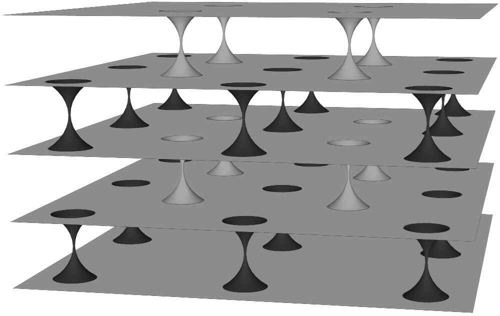
Refer to caption
Figure 1. An N=5N=5 initial surface, cut by four hemispheres and viewed in the (x,y,z)(\mathrm{x},\mathrm{y},\mathrm{z}) coordinate system; for clarity the picture grossly exaggerates the ratio, which in fact tends to 00 with large mm, of the vertical spacing between the tori to the horizontal spacing between the catenoids.

Half-catenoids bent to planes

We shall make frequent use of cutoff functions throughout the construction, so we fix now a smooth, nondecreasing Ψ:ℝ→[0,1]\Psi:\mathbb{R}\to[0,1] with Ψ\Psi identically 00 on (−∞,−1](-\infty,-1], identically 11 on [1,∞)[1,\infty), and such that Ψ−12\Psi-\frac{1}{2} is odd. We then define, for any a,b∈ℝa,b\in\mathbb{R}, the function ψ⁡[a,b]:ℝ→[0,1]\psi\left[a,b\right]:\mathbb{R}\to[0,1] by

(2.4) ψ⁡[a,b]:=Ψ∘La,b,\psi\left[a,b\right]:=\Psi\circ L_{a,b},

where La,b:ℝ→ℝL_{a,b}:\mathbb{R}\to\mathbb{R} is the linear function satisfying L⁡(a)=−3L(a)=-3 and L⁡(b)=3L(b)=3.

We write B⁡[(x,y),r]B[(x,y),r] for the open Euclidean disc in ℝ2\mathbb{R}^{2} with radius rr and center (x,y)(x,y). Given X,Y,τ>0X,Y,\tau>0 with τ<min⁡{X,Y}\tau<\min\{X,Y\}, we set

(2.5) 𝕋X,Y,τ:=([−X,X]×[−Y,Y])\B⁡[(0,0),τ],\mathbb{T}_{X,Y,\tau}:=\left([-X,X]\times[-Y,Y]\right)\backslash B[(0,0),\tau],

a solid rectangle with a disc removed from its center. Given also zK,zT∈ℝ\mathrm{z}_{K},\mathrm{z}_{T}\in\mathbb{R} and R>τR>\tau with 2​R<min⁡{X,Y}2R<\min\{X,Y\}, we define the function ϕ⁡[zK,zT,R,X,Y,τ]:𝕋X,Y,τ→ℝ\phi[\mathrm{z}_{K},\mathrm{z}_{T},R,X,Y,\tau]:\mathbb{T}_{X,Y,\tau}\to\mathbb{R} by

(2.6) ϕ⁡[zK,zT,R,X,Y,τ]​(x,y):=\displaystyle\phi[\mathrm{z}_{K},\mathrm{z}_{T},R,X,Y,\tau](\mathrm{x},\mathrm{y}):= zK+(zT−zK)​ψ​[R,2​R]​(x2+y2)\displaystyle\mathrm{z}_{K}+(\mathrm{z}_{T}-\mathrm{z}_{K})\psi\left[R,2R\right]\left(\sqrt{\mathrm{x}^{2}+\mathrm{y}^{2}}\right)
+sgn⁡(zT−zK)​(τ​arcosh⁡x2+y2τ)​ψ​[2​R,R]​(x2+y2),\displaystyle+\operatorname{sgn}(\mathrm{z}_{T}-\mathrm{z}_{K})\left(\tau\operatorname{arcosh}\frac{\sqrt{\mathrm{x}^{2}+\mathrm{y}^{2}}}{\tau}\right)\psi\left[2R,R\right]\left(\sqrt{\mathrm{x}^{2}+\mathrm{y}^{2}}\right),

where arcosh:[1,∞)→[0,∞)\operatorname{arcosh}:[1,\infty)\to[0,\infty) is the inverse of the restriction to [0,∞)[0,\infty) of the hyperbolic cosine function and the sign function sgn:ℝ→ℝ\operatorname{sgn}:\mathbb{R}\to\mathbb{R} takes the value 11 when its argument is nonnegative and the value −1-1 otherwise. Thus, inside the cylinder of radius RR about the z\mathrm{z}-axis the graph of ϕ\phi coincides with the portion between the planes z=zK\mathrm{z}=\mathrm{z}_{K} and z=zT\mathrm{z}=\mathrm{z}_{T} of the catenoid with vertical axis, center (0,0,zK)\left(0,0,\mathrm{z}_{K}\right), and waist radius τ\tau, while outside the cylinder of radius 2​R2R about the z\mathrm{z}-axis it coincides with the solid rectangle [−X,X]×[−Y,Y]×{z=zT}[-X,X]\times[-Y,Y]\times\left\{\mathrm{z}=\mathrm{z}_{T}\right\}. In between these two cylinders the cutoff function is used to bend the end of the half-catenoid to become exactly horizontal. With the additional data (x0,y0)∈ℝ2(\mathrm{x}_{0},\mathrm{y}_{0})\in\mathbb{R}^{2} we define the embedding

(2.7) Te​x​t​[(x0,y0),zK,zT,R,X,Y,τ]:𝕋X,Y,τ→ℝ3​ by\displaystyle T_{ext}[(\mathrm{x}_{0},\mathrm{y}_{0}),\mathrm{z}_{K},\mathrm{z}_{T},R,X,Y,\tau]:\mathbb{T}_{X,Y,\tau}\to\mathbb{R}^{3}\mbox{ by}
Te​x​t​(x,y):=(x0+x,y0+y,ϕ⁡[zK,zT,R,X,Y,τ]​(x,y)),\displaystyle T_{ext}(\mathrm{x},\mathrm{y}):=\left(\mathrm{x}_{0}+\mathrm{x},\mathrm{y}_{0}+\mathrm{y},\phi[\mathrm{z}_{K},\mathrm{z}_{T},R,X,Y,\tau](\mathrm{x},\mathrm{y})\right),

whose image is the graph of ϕ\phi translated by (x0,y0,0)(\mathrm{x}_{0},\mathrm{y}_{0},0).

Given also zK′∈ℝ\mathrm{z}_{K}^{\prime}\in\mathbb{R} along with τ′>0\tau^{\prime}>0, now assuming max⁡{τ,τ′}<R<14​min⁡{X,Y}\max\{\tau,\tau^{\prime}\}<R<\frac{1}{4}\min\{X,Y\}, we set

(2.8) 𝕋X,Y,τ,τ′:=([−X,X]×[−Y,Y])\(B⁡[(−X2,−Y2),τ]∪B⁡[(X2,Y2),τ′]),\mathbb{T}_{X,Y,\tau,\tau^{\prime}}:=([-X,X]\times[-Y,Y])\left\backslash\left(B\left[\left(-\frac{X}{2},-\frac{Y}{2}\right),\tau\right]\cup B\left[\left(\frac{X}{2},\frac{Y}{2}\right),\tau^{\prime}\right]\right)\right.,

and we define the embedding

(2.9) Ti​n​t[(x0,y0),zK,zK′,zT,R,X,Y,τ,τ′]:𝕋X,Y,τ,τ′→ℝ3 by\displaystyle T_{int}[(\mathrm{x}_{0},\mathrm{y}{{}_{0}}),\mathrm{z}_{K},\mathrm{z}_{K}^{\prime},\mathrm{z}_{T},R,X,Y,\tau,\tau^{\prime}]:\mathbb{T}_{X,Y,\tau,\tau^{\prime}}\to\mathbb{R}^{3}\mbox{ by}
Ti​n​t​(x,y):=\displaystyle T_{int}(\mathrm{x},\mathrm{y}):=
{(x0+x,y0+y,ϕ⁡[zK,zT,R,X2,Y2,τ]​(x+X2,y+Y2))​ for ​(x,y)∈[−X,0]×[−Y,0](x0+x,y0+y,ϕ⁡[zK′,zT,R,X2,Y2,τ′]​(x−X2,y−Y2))​ for ​(x,y)∈[0,X]×[0,Y](x0+x,y0+y,zT)​ everywhere else. \displaystyle\begin{cases}\left(\mathrm{x}_{0}+\mathrm{x},\mathrm{y}_{0}+\mathrm{y},\phi\left[\mathrm{z}_{K},\mathrm{z}_{T},R,\frac{X}{2},\frac{Y}{2},\tau\right]\left(\mathrm{x}+\frac{X}{2},\mathrm{y}+\frac{Y}{2}\right)\right)\mbox{ for }(\mathrm{x},\mathrm{y})\in[-X,0]\times[-Y,0]\\ \left(\mathrm{x}_{0}+\mathrm{x},\mathrm{y}_{0}+\mathrm{y},\phi\left[\mathrm{z}_{K}^{\prime},\mathrm{z}_{T},R,\frac{X}{2},\frac{Y}{2},\tau^{\prime}\right]\left(\mathrm{x}-\frac{X}{2},\mathrm{y}-\frac{Y}{2}\right)\right)\mbox{ for }(\mathrm{x},\mathrm{y})\in[0,X]\times[0,Y]\\ (\mathrm{x}_{0}+\mathrm{x},\mathrm{y}_{0}+\mathrm{y},\mathrm{z}_{T})\mbox{ everywhere else. }\end{cases}

Thus the image of Ti​n​tT_{int} looks like a solid 2​X×2​Y2X\times 2Y rectangle in the z=zT\mathrm{z}=\mathrm{z}_{T} plane with two discs centered at (x0,y0,zT)±(X2,Y2,0)\left(\mathrm{x}_{0},\mathrm{y}_{0},\mathrm{z}_{T}\right)\pm\left(\frac{X}{2},\frac{Y}{2},0\right) replaced by catenoidal annuli terminating on waist circles at heights zK′\mathrm{z}_{K}^{\prime} and zK\mathrm{z}_{K}.

The initial surfaces will be built from various applications of Te​x​tT_{ext}, for extreme or outermost tori and adjoining half-catenoids, and of Ti​n​tT_{int}, for the intermediate tori and pairs of adjoining half-catenoids. The horizontal positions of the catenoids (the values of (x0,y0)(\mathrm{x}_{0},\mathrm{y}_{0}) in the parametrizations above) and the dimensions (XX and YY) of the parametrizing solid rectangles (or equivalently the lattice edges) will be set directly by the data kk, ℓ\ell, and mm. The radii of the annuli of transition (determined by RR) will be chosen on the order of min⁡{X,Y}\min\{X,Y\} (but smaller than it by a wide enough margin that the images of Te​x​tT_{ext} and Ti​n​tT_{int} are horizontal near their boundaries as assumed above). There remain N−1N-1 selections of waist radii (τ\tau and τ′\tau^{\prime}) and N−1N-1 more of waist heights (zK\mathrm{z}_{K} and zK′\mathrm{z}_{K}^{\prime}). Balancing conditions studied in the next section allow for the estimation of the values these 2​N−22N-2 unknowns must assume for the construction to succeed, but their precise specification is made by the ζ\zeta and ξ\xi parameters described in Section 1. Matching conditions will then fix the height zT\mathrm{z}_{T} of each torus, by requiring these heights to agree with the heights of the adjoining catenoids where they meet the transition annuli, in the case of the extreme tori, or to agree with the average of the heights of the upper and lower catenoids at the transition circles they adjoin, in the case of the intermediate tori.

The hierarchy of data

For any positive integers kk, ℓ\ell, and N≥2N\geq 2 the first phase of the construction produces a sequence, indexed by mm, of (2​N−2)(2N-2)-parameter families of initial surfaces. In order to obtain adequate estimates for the initial mean curvature, the linearized operator, and the nonlinear terms, we will routinely make the assumption that mm is as large as needed in terms of kk, ℓ\ell, NN, and all of the parameters. Of course we expect the ultimate parameter choices themselves to depend on mm, so, in taking mm large as just described, it is necessary to assume that the parameters are all bounded in absolute value by a constant c>0c>0 independent of mm. Naturally we do not yet know what range is needed for the parameters, but eventually we will be able to pick cc in terms of kk, ℓ\ell, and NN so that for every sufficiently large mm we will be able to find parameters bounded by cc so that the corresponding initial surface can be perturbed to minimality.

To continue with the definition of the intial surfaces we assume we are given integers k,ℓ,m≥1k,\ell,m\geq 1 and N≥2N\geq 2 as well as a constant c>0c>0 and parameters ζ,ξ∈[−c,c]N−1\zeta,\xi\in[-c,c]^{N-1}. For notational simplicity we assume

(2.10) k≤ℓk\leq\ell

and we write n=n⁡[N]n=n[N] for the greatest integer no greater than N/2N/2, so that

(2.11) N={2​n​ when N is even2​n+1​ when N is odd.N=\begin{cases}2n\mbox{ when $N$ is even}\\ 2n+1\mbox{ when $N$ is odd.}\end{cases}

We acknowledge a certain redundancy in the minimal surfaces ultimately exhibited, one which is easily removed by taking kk and ℓ\ell relatively prime.

Catenoidal radii and vertical specifications

Modulo the symmetries that we will impose when defining our initial surfaces we have N−1N-1 catenoidal waist radii τ1,…,τN−1\tau_{1},\ldots,\tau_{N-1} to prescribe, one for each pair of adjacent tori to be joined. Their selection is critical to the success of the construction, and the next section (Section 3) is devoted in part to making a viable choice. Specifically, in Lemma 3.18, when N≥4N\geq 4, we will determine a collection {bj}j=2n\{b_{j}\}_{j=2}^{n} of n−1n-1 positive real numbers (recalling (2.11) just above), which in turn we will use in conjunction with the ζ\zeta parameters to set the waist radii of our catenoidal tunnels. Each bjb_{j} will be a function of kk, ℓ\ell, NN, and mm but (for large mm) will have an upper bound and a positive lower bound depending only on NN; in particular b2b_{2} will have an upper bound depending on NN but always strictly less than 22. Of course in the simpler cases N=2N=2 and N=3N=3 we have n−1=0n-1=0, but it is nevertheless notationally convenient to set b2:=0b_{2}:=0 when N=2N=2 and b2:=1b_{2}:=1 when N=3N=3. We emphasize that each bj=bj​[N,k,ℓ,m]b_{j}=b_{j}[N,k,\ell,m] depends at least on NN and generally on the data kk, ℓ\ell, and mm as well, but for brevity in our notation we will frequently suppress the expression of this dependence, as we do for many other quantities of interest. To summarize:

(2.12) b2[N=2,k,ℓ,m]:=0,b2[N=3,k,ℓ,m]:=1,and for N≥4\displaystyle b_{2}[N=2,k,\ell,m]:=0,\qquad b_{2}[N=3,k,\ell,m]:=1,\qquad\mbox{and for $N\geq 4$}
{bi​[N,k,ℓ,m]}i=2n​ is determined in Lemma 3.18 (recalling (2.11)),\displaystyle\{b_{i}[N,k,\ell,m]\}_{i=2}^{n}\mbox{ is determined in Lemma \ref{cilemma} (recalling \eqref{ndef})},
so there exists a constant C⁡[N,k,ℓ]>0 such that for N≥4\displaystyle\mbox{so there exists a constant $C[N,k,\ell]>0$ such that for $N\geq 4$}
1<max⁡{bi}i=2n<C⁡[N,k,ℓ]andb2≤2−1/C⁡[N,k,ℓ]\displaystyle 1<\max\{b_{i}\}_{i=2}^{n}<C[N,k,\ell]\quad\mbox{and}\quad b_{2}\leq 2-1/C[N,k,\ell]
whenever m is large enough in terms of N.\displaystyle\mbox{whenever $m$ is large enough in terms of $N$}.

Having identified these numbers, we first define the collection {τ¯i}i=1N−1\{\underline{\tau}_{i}\}_{i=1}^{N-1} of waist radii when ζ=0\zeta=0 by

(2.13) τ¯i=τ¯i​[N,k,ℓ,m]:={110​ℓ​m​e−k​ℓ​m24​π​(1−12​b2​[N,k,ℓ,m])​ for ​i=1bi​[N,k,ℓ,m]​τ¯1​[N,k,ℓ,m]​ for ​2≤i≤nτ¯N−i​[N,k,ℓ,m]​ for ​n+1≤i≤N−1\underline{\tau}_{i}=\underline{\tau}_{i}[N,k,\ell,m]:=\begin{cases}\frac{1}{10\ell m}e^{-\frac{k\ell m^{2}}{4\pi}\left(1-\frac{1}{2}b_{2}[N,k,\ell,m]\right)}\mbox{ for }i=1\\ b_{i}[N,k,\ell,m]\underline{\tau}_{1}[N,k,\ell,m]\mbox{ for }2\leq i\leq n\\ \underline{\tau}_{N-i}[N,k,\ell,m]\mbox{ for }n+1\leq i\leq N-1\end{cases}

(recalling (2.11)) and then for general ζ\zeta we define the radii

(2.14) τi=τi​[N,k,ℓ,m,ζ]:={eζ1​τ¯1​[N,k,ℓ,m]​ for ​i=1eζ1+k−1​ℓ−1​m−2​ζi​τ¯i​[N,k,ℓ,m]​ for ​1<i<N.\tau_{i}=\tau_{i}[N,k,\ell,m,\zeta]:=\begin{cases}e^{\zeta_{1}}\underline{\tau}_{1}[N,k,\ell,m]\mbox{ for }i=1\\ e^{\zeta_{1}+k^{-1}\ell^{-1}m^{-2}\zeta_{i}}\underline{\tau}_{i}[N,k,\ell,m]\mbox{ for }1<i<N.\end{cases}

We next define the NN heights zi=zi​[N,k,ℓ,m,ζ,ξ]\mathrm{z}_{i}=\mathrm{z}_{i}[N,k,\ell,m,\zeta,\xi] of the tori by

(2.15) z1:=τ1​ξ1−2Nmod2​τn​ln⁡110​ℓ​m​τn−2​∑j=1n−1τj​ln⁡110​ℓ​m​τj,\displaystyle\mathrm{z}_{1}:=\tau_{1}\xi_{1}-2^{N\bmod 2}\tau_{n}\ln\frac{1}{10\ell m\tau_{n}}-2\displaystyle{\sum_{j=1}^{n-1}}\tau_{j}\ln\frac{1}{10\ell m\tau_{j}},
zN:=τN−1​ξN−1−2Nmod2​τn​ln⁡110​ℓ​m​τn+2​∑j=nN−1τj​ln⁡110​ℓ​m​τj, and for 1<i<N\displaystyle\mathrm{z}_{N}:=\tau_{N-1}\xi_{N-1}-2^{N\bmod 2}\tau_{n}\ln\frac{1}{10\ell m\tau_{n}}+2\displaystyle{\sum_{j=n}^{N-1}}\tau_{j}\ln\frac{1}{10\ell m\tau_{j}},\mbox{ and for $1<i<N$}
zi:=τi−1​ξi−1+τi​ξi2−2Nmod2​τn​ln⁡110​ℓ​m​τn+2​∑j=1i−1τj​ln⁡110​ℓ​m​τj−2​∑j=1n−1τj​ln⁡110​ℓ​m​τj,\displaystyle\mathrm{z}_{i}:=\frac{\tau_{i-1}\xi_{i-1}+\tau_{i}\xi_{i}}{2}-2^{N\bmod 2}\tau_{n}\ln\frac{1}{10\ell m\tau_{n}}+2\displaystyle{\sum_{j=1}^{i-1}}\tau_{j}\ln\frac{1}{10\ell m\tau_{j}}-2\displaystyle{\sum_{j=1}^{n-1}}\tau_{j}\ln\frac{1}{10\ell m\tau_{j}},

and the N−1N-1 heights ziK=ziK​[N,k,ℓ,m,ζ,ξ]\mathrm{z}_{i}^{K}=\mathrm{z}_{i}^{K}[N,k,\ell,m,\zeta,\xi] of the catenoids’ centers by

(2.16) ziK:=τi​ξi+τi​ln​110​ℓ​m​τi+2​∑j=1i−1τj​ln​110​ℓ​m​τj−2​∑j=1n−1τj​ln​110​ℓ​m​τj−2Nmod2​τn​ln​110​ℓ​m​τn\mathrm{z}_{i}^{K}:=\tau_{i}\xi_{i}+\tau_{i}\ln\frac{1}{10\ell m\tau_{i}}+2\displaystyle{\sum_{j=1}^{i-1}}\tau_{j}\ln\frac{1}{10\ell m\tau_{j}}-2\sum_{j=1}^{n-1}\tau_{j}\ln\frac{1}{10\ell m\tau_{j}}-2^{N\bmod 2}\tau_{n}\ln\frac{1}{10\ell m\tau_{n}}

for 1≤i≤N−11\leq i\leq N-1.

Equivalently,

(2.17) ziK​[N,k,ℓ,m,ζ,ξ]=ziK​[N,k,ℓ,m,ζ,0]+τi​ξi​ for 1≤i≤N−1,\displaystyle\mathrm{z}_{i}^{K}[N,k,\ell,m,\zeta,\xi]=\mathrm{z}_{i}^{K}[N,k,\ell,m,\zeta,0]+\tau_{i}\xi_{i}\mbox{ for $1\leq i\leq N-1$},
zi​[N,k,ℓ,m,ζ,ξ]=zi​[N,k,ℓ,m,ζ,0]+{τ1​ξ1​ for i=1τN−1​ξN−1​ for i=N12​(τi−1​ξi−1+τi​ξi)​ for 1<i<N,\displaystyle\mathrm{z}_{i}[N,k,\ell,m,\zeta,\xi]=\mathrm{z}_{i}[N,k,\ell,m,\zeta,0]+\begin{cases}\tau_{1}\xi_{1}\mbox{ for $i=1$}\\ \tau_{N-1}\xi_{N-1}\mbox{ for $i=N$}\\ \frac{1}{2}\left(\tau_{i-1}\xi_{i-1}+\tau_{i}\xi_{i}\right)\mbox{ for $1<i<N$,}\end{cases}
ziK​[N,k,ℓ,m,ζ,0]=zi​[N,k,ℓ,m,ζ,0]+τi​ln⁡110​ℓ​m​τi​ for 1≤i≤N−1,\displaystyle\mathrm{z}_{i}^{K}[N,k,\ell,m,\zeta,0]=\mathrm{z}_{i}[N,k,\ell,m,\zeta,0]+\tau_{i}\ln\frac{1}{10\ell m\tau_{i}}\mbox{ for $1\leq i\leq N-1$},
zi+1​[N,k,ℓ,m,ζ,0]=zi​[N,k,ℓ,m,ζ,0]+2​τi​ln⁡110​ℓ​m​τi​ for 1≤i≤N−1, and\displaystyle\mathrm{z}_{i+1}[N,k,\ell,m,\zeta,0]=\mathrm{z}_{i}[N,k,\ell,m,\zeta,0]+2\tau_{i}\ln\frac{1}{10\ell m\tau_{i}}\mbox{ for $1\leq i\leq N-1$, and}
znK​[2​n,k,ℓ,m,ζ,0]=zn+1​[2​n+1,k,ℓ,m,ζ,0]=0​ (recalling (2.11)).\displaystyle\mathrm{z}_{n}^{K}[2n,k,\ell,m,\zeta,0]=\mathrm{z}_{n+1}[2n+1,k,\ell,m,\zeta,0]=0\mbox{ (recalling \eqref{ndef})}.

From definition (2.14)

(2.18) ln⁡110​ℓ​m​τi=k​ℓ4​π​(1−b22)​m2−ζ1−(1−δi​1)​(ln⁡bi+ζik​ℓ​m2)​ for 1≤i≤N−1,\ln\frac{1}{10\ell m\tau_{i}}=\frac{k\ell}{4\pi}\left(1-\frac{b_{2}}{2}\right)m^{2}-\zeta_{1}-\left(1-\delta_{i1}\right)\left(\ln b_{i}+\frac{\zeta_{i}}{k\ell m^{2}}\right)\mbox{ for $1\leq i\leq N-1$},

where δi​1={1​ if i=10​ otherwise,\delta_{i1}=\left\{\begin{smallmatrix}1\mbox{ if $i=1$}\\ 0\mbox{ otherwise,}\end{smallmatrix}\right. so by taking mm sufficiently large in terms of ζ\zeta, ξ\xi, and each bib_{i} (which according to (2.12) satisfy bounds depending on just NN, kk, and ℓ\ell), we can make every zi\mathrm{z}_{i} and ziK\mathrm{z}_{i}^{K} as close to 00 as desired and we can also guarantee that

(2.19) zi​[N,k,ℓ,m,ζ,ξ]<ziK​[N,k,ℓ,m,ζ,0]<zi+1​[N,k,ℓ,m,ζ,ξ]​ for 1≤i≤N−1.\mathrm{z}_{i}[N,k,\ell,m,\zeta,\xi]<\mathrm{z}_{i}^{K}[N,k,\ell,m,\zeta,0]<\mathrm{z}_{i+1}[N,k,\ell,m,\zeta,\xi]\mbox{ for $1\leq i\leq N-1$}.

The definitions (2.15) and (2.16) can be understood as implementing the matching conditions mentioned earlier as well as the vertical offsets introduced by the ξ\xi parameters. Here the logarithm is used—merely because it simplifies some expressions later—to capture the dominant part of the inverse hyperbolic cosine function for large values of its argument. Thus each logarithmic term, ignoring any powers of 22 appearing as prefactors, represents the height achieved by a corresponding catenoid above its waist plane a distance 110​ℓ​m\frac{1}{10\ell m} from its axis, where the catenoids are meant to transition to planes (tori under Φ\Phi). The factor of 10​ℓ10\ell is chosen—1010 somewhat arbitrarily and ℓ\ell because we assume k≤ℓk\leq\ell—to ensure the transition is completed on the order—m−1m^{-1}—of the lattice spacing but well away from neighboring catenoids. From the identity

(2.20) arcosh⁡x=ln⁡x+ln⁡(1+1−x−2)\operatorname{arcosh}x=\ln x+\ln\left(1+\sqrt{1-x^{-2}}\right)

we have the estimate

(2.21) |τi​arcosh⁡110​ℓ​m​τi−τi​ln⁡110​ℓ​m​τi|≤τi​ln⁡2,\left\lvert\tau_{i}\operatorname{arcosh}\frac{1}{10\ell m\tau_{i}}-\tau_{i}\ln\frac{1}{10\ell m\tau_{i}}\right\rvert\leq\tau_{i}\ln 2,

so our very substitution of ln\ln for arcosh\operatorname{arcosh} introduces additional height mismatch (beyond that contributed by the ξ\xi parameters) where catenoidal annuli connect to tori, but one whose ratio to τ1\tau_{1} is obviously bounded independently of the ζ\zeta and ξ\xi parameters.

Refer to caption
Figure 2. A schematic profile of two N=4N=4 initial surfaces. The surface on the left has ξ1=ξ2=ξ3=0\xi_{1}=\xi_{2}=\xi_{3}=0, while the one on the right has nonzero values for all three of these parameters, with τ1​ξ1=τ2​ξ2≠τ3​ξ3\tau_{1}\xi_{1}=\tau_{2}\xi_{2}\neq\tau_{3}\xi_{3}, resulting in dislocation at the third torus from the bottom and nowhere else. The figure is not drawn to scale. In fact (see especially (2.14) and (2.18)) the vertical spacing τi​ln⁡110​ℓ​m​τi\tau_{i}\ln\frac{1}{10\ell m\tau_{i}} is of order m2​τ1m^{2}\tau_{1} and limm→∞m2​τ1m−1=0\lim_{m\to\infty}\frac{m^{2}\tau_{1}}{m^{-1}}=0. Note also that the schematic does not attempt to convey the height mismatch, of order τ1\tau_{1}, arising from the approximation of arcosh\operatorname{arcosh} by ln\ln (see (2.21)), because, unlike the dislocations controlled by ξ\xi, it plays no role in the construction.

Symmetries and horizontal specifications

By the definition (2.1) of 𝕋\mathbb{T} as the locus of points in 𝕊3\mathbb{S}^{3} equidistant from C1C_{1} and C2C_{2}, the symmetry group 𝒢s​y​m​[𝕋]\mathscr{G}_{sym}[\mathbb{T}] of 𝕋\mathbb{T} in 𝕊3\mathbb{S}^{3}, that is the subgroup of O⁡(4)O(4) preserving 𝕋\mathbb{T} as a set, is precisely the symmetry group of C1∪C2C_{1}\cup C_{2}. Accordingly 𝒢s​y​m​[𝕋]\mathscr{G}_{sym}[\mathbb{T}] is generated by the set of all reflections through great spheres containing either C1C_{1} or C2C_{2} together with the set of reflections through any great circle equidistant from C1C_{1} and C2C_{2} (so contained in a plane of the form {z1=ei​θz2}\{z_{1}=e^{i\theta}z_{2}\} or {z1=ei​θz¯2}\{z_{1}=e^{i\theta}\overline{z}_{2}\}) and therefore lying on 𝕋\mathbb{T}. (Here reflection through a great sphere (or circle) refers to the element of O⁡(4)O(4) that identically preserves the 33-space (or 22-plane) containing that sphere (or circle) and reflects the orthogonal complement through the origin.) Consequently 𝒢s​y​m​[𝕋]\mathscr{G}_{sym}[\mathbb{T}] also includes rotation in C1C_{1} and C2C_{2} by any angles as well as reflection through any great circle orthogonally intersecting 𝕋\mathbb{T} (and C1C_{1} and C2C_{2}).

We equip ℂ2\mathbb{C}^{2}, C1C_{1}, and C2C_{2} with their standard orientations and, given an oriented circle CC in 𝕊3\mathbb{S}^{3}, we write 𝖱Cθ\mathsf{R}_{C}^{\theta} for rotation by θ\theta about CC, which by definition is the element of O⁡(4)O(4) fixing the plane containing CC pointwise and rotating its orthogonal complement by angle θ\theta in the direction consistent with the induced orientation. We write 𝖷¯\underline{\mathsf{X}} for reflection through the great sphere with equator C2C_{2} and poles (±1,0)(\pm 1,0), 𝖸¯\underline{\mathsf{Y}} for reflection through the great sphere with equator C1C_{1} and poles (0,±1)(0,\pm 1), and 𝖹¯\underline{\mathsf{Z}} for reflection through the great circle in the plane {z1=z2}\{z_{1}=z_{2}\} (so 𝖹¯=𝖱{z1=z2}∩𝕊3π\underline{\mathsf{Z}}=\mathsf{R}_{\{z_{1}=z_{2}\}\cap\mathbb{S}^{3}}^{\pi}). Thus (writing z¯\overline{z} for the complex conjugate of z∈ℂz\in\mathbb{C})

(2.22) 𝖷¯(z1,z2)=(z1¯,z2),𝖸¯(z1,z2)=(z1,z2¯),𝖹¯(z1,z2)=(z2,z1),\displaystyle\underline{\mathsf{X}}(z_{1},z_{2})=(\overline{z_{1}},z_{2}),\qquad\underline{\mathsf{Y}}(z_{1},z_{2})=(z_{1},\overline{z_{2}}),\qquad\underline{\mathsf{Z}}(z_{1},z_{2})=(z_{2},z_{1}),
𝖱C2θ​(z1,z2)=(ei​θ​z1,z2),and𝖱C1θ​(z1,z2)=(z1,ei​θ​z2)\displaystyle\mathsf{R}_{C_{2}}^{\theta}(z_{1},z_{2})=(e^{i\theta}z_{1},z_{2}),\qquad\mbox{and}\qquad\mathsf{R}_{C_{1}}^{\theta}(z_{1},z_{2})=(z_{1},e^{i\theta}z_{2})

and

(2.23) 𝒢s​y​m[𝕋]=⟨𝖷¯,𝖸¯,𝖹¯,𝖱C1θ1,𝖱C2θ2:θ1,θ2∈ℝ⟩,\mathscr{G}_{sym}[\mathbb{T}]=\left\langle\underline{\mathsf{X}},\underline{\mathsf{Y}},\underline{\mathsf{Z}},\mathsf{R}_{C_{1}}^{\theta_{1}},\mathsf{R}_{C_{2}}^{\theta_{2}}\;:\;\theta_{1},\theta_{2}\in\mathbb{R}\right\rangle,

where the right-hand side is the subgroup of O⁡(4)O(4) generated by the elements the angled brackets enclose.

Recalling (2.2), we also name some elements of O⁡(3)O(3) preserving the domain of Φ\Phi and the pullback metric Φ∗gS\Phi^{*}g_{{}_{S}}: we write 𝖳^x​-axish\widehat{\mathsf{T}}_{\mathrm{x}\text{-axis}}^{h} and 𝖳^y​-axish\widehat{\mathsf{T}}_{\mathrm{y}\text{-axis}}^{h} for translation by (real number) hh in the (positive) x\mathrm{x} and y\mathrm{y} directions respectively, 𝖷¯^\widehat{\underline{\mathsf{X}}} and 𝖸¯^\widehat{\underline{\mathsf{Y}}} for reflection through the x=0\mathrm{x}=0 and y=0\mathrm{y}=0 planes respectively, and 𝖹¯^\widehat{\underline{\mathsf{Z}}} for reflection through the line x=y\mathrm{x}=\mathrm{y} in the plane z=0\mathrm{z}=0. Thus

(2.24) 𝖷¯^(x,y,z)=(−x,y,z),𝖸¯^(x,y,z)=(x,−y,z),𝖹¯^(x,y,z)=(y,x,−z),\displaystyle\widehat{\underline{\mathsf{X}}}(\mathrm{x},\mathrm{y},\mathrm{z})=(-\mathrm{x},\mathrm{y},\mathrm{z}),\qquad\widehat{\underline{\mathsf{Y}}}(\mathrm{x},\mathrm{y},\mathrm{z})=(\mathrm{x},-\mathrm{y},\mathrm{z}),\qquad\widehat{\underline{\mathsf{Z}}}(\mathrm{x},\mathrm{y},\mathrm{z})=(\mathrm{y},\mathrm{x},-\mathrm{z}),
𝖳^x​-axish​(x,y,z)=(x+h,y,z),and𝖳^y​-axish​(x,y,z)=(x,y+h,z).\displaystyle\widehat{\mathsf{T}}_{\mathrm{x}\text{-axis}}^{h}(\mathrm{x},\mathrm{y},\mathrm{z})=(\mathrm{x}+h,\mathrm{y},\mathrm{z}),\qquad\mbox{and}\qquad\widehat{\mathsf{T}}_{\mathrm{y}\text{-axis}}^{h}(\mathrm{x},\mathrm{y},\mathrm{z})=(\mathrm{x},\mathrm{y}+h,\mathrm{z}).

It is then easy to verify the relations

(2.25) Φ∘𝖷¯^=𝖷¯∘Φ,Φ∘𝖸¯^\displaystyle\Phi\circ\widehat{\underline{\mathsf{X}}}=\underline{\mathsf{X}}\circ\Phi,\qquad\Phi\circ\widehat{\underline{\mathsf{Y}}} =𝖸¯∘Φ,Φ∘𝖹¯^=𝖹¯∘Φ,\displaystyle=\underline{\mathsf{Y}}\circ\Phi,\qquad\Phi\circ\widehat{\underline{\mathsf{Z}}}=\underline{\mathsf{Z}}\circ\Phi,
Φ∘𝖳^x​-axish=𝖱C22​h∘Φ,\displaystyle\Phi\circ\widehat{\mathsf{T}}_{\mathrm{x}\text{-axis}}^{h}=\mathsf{R}_{C_{2}}^{\sqrt{2}h}\circ\Phi, andΦ∘𝖳^y​-axish=𝖱C12​h∘Φ for every h∈ℝ,\displaystyle\mbox{and}\qquad\Phi\circ\widehat{\mathsf{T}}_{\mathrm{y}\text{-axis}}^{h}=\mathsf{R}_{C_{1}}^{\sqrt{2}h}\circ\Phi\quad\mbox{ for every $h\in\mathbb{R}$},

which play an essential role in identifying the symmetries of the initial surfaces, defined via Φ\Phi, and in exploiting these symmetries when solving the linearized problem.

Each initial surface will be built to be invariant under a certain subgroup of 𝒢s​y​m​[T]\mathscr{G}_{sym}[T], with the symmetries of 𝕋\mathbb{T} broken in several ways. Recall that each initial surface is to be obtained by gluing together a collection of constant-mean-curvature tori coaxial with 𝕋\mathbb{T} using a collection of catenoidal annuli. Since among these tori only 𝕋\mathbb{T} itself is equidistant from C1C_{1} and C2C_{2}, the symmetry group of every other such torus is just the subgroup ⟨𝖷¯,𝖸¯,𝖱C1θ1,𝖱C2θ2:θ1,θ2∈ℝ⟩\left\langle\underline{\mathsf{X}},\underline{\mathsf{Y}},\mathsf{R}_{C_{1}}^{\theta_{1}},\mathsf{R}_{C_{2}}^{\theta_{2}}\;:\;\theta_{1},\theta_{2}\in\mathbb{R}\right\rangle of horizontal symmetries of 𝕋\mathbb{T}. If the toral components of an initial surface are not arranged symmetrically about 𝕋\mathbb{T}, then of course the initial surface itself cannot possess any vertical symmetries. The arrangement of the catenoidal tunnels may also be inconsistent with vertical symmetry and inevitably breaks the continuous horizontal symmetries, leaving only a discrete subgroup. In this construction we impose the group

(2.26) 𝒢=𝒢⁡[k,ℓ,m]:=⟨𝖱C22​πk​m,𝖱C12​πℓ​m,𝖷¯,𝖸¯⟩<𝒢s​y​m​[𝕋]<O⁡(4),\mathscr{G}=\mathscr{G}[k,\ell,m]:=\left\langle\mathsf{R}_{C_{2}}^{\frac{2\pi}{km}},\,\mathsf{R}_{C_{1}}^{\frac{2\pi}{\ell m}},\,\underline{\mathsf{X}},\,\underline{\mathsf{Y}}\right\rangle<\mathscr{G}_{sym}[\mathbb{T}]<O(4),

which is the subgroup of O⁡(4)O(4) preserving the set of k​mkmth roots of unity on C1C_{1} as well as (separately) the set of ℓ​m\ell mth roots of unity on C2C_{2}; as such, 𝒢⁡[k,ℓ,m]\mathscr{G}[k,\ell,m] is therefore isomorphic to Dk​m×Dℓ​mD_{km}\times D_{\ell m}, where DqD_{q} is the dihedral group of order 2​q2q. We will sometimes write 𝒢\mathscr{G} in place of 𝒢⁡[k,ℓ,m]\mathscr{G}[k,\ell,m] when there is no danger of confusion.

The catenoidal tunnels connecting each pair of adjacent tori will be placed, via Φ\Phi, so as to take their centers on the great circles orthogonally intersecting 𝕋\mathbb{T} at the sites of a 𝒢⁡[k,ℓ,m]\mathscr{G}[k,\ell,m]-invariant k​m×ℓ​mkm\times\ell m rectangular lattice. There are precisely four such lattices, namely the 𝒢⁡[k,ℓ,m]\mathscr{G}[k,\ell,m] orbits

(2.27) Lσx,σy=Lσx,σy​[k,ℓ,m]:=𝒢⁡[k,ℓ,m]​(ei​σx​π/(k​m),ei​σy​π/(ℓ​m))=Φ⁡(L^σx,σy×{0}), where\displaystyle L_{\sigma_{\mathrm{x}},\sigma_{\mathrm{y}}}=L_{\sigma_{\mathrm{x}},\sigma_{\mathrm{y}}}[k,\ell,m]:=\mathscr{G}[k,\ell,m]\left(e^{i\sigma_{\mathrm{x}}\pi/(km)},e^{i\sigma_{\mathrm{y}}\pi/(\ell m)}\right)=\Phi\left(\widehat{L}_{\sigma_{\mathrm{x}},\sigma_{\mathrm{y}}}\times\{0\}\right),\mbox{ where}
L^σx,σy=L^σx,σy[k,ℓ,m]:={(σx​π2​k​m+nx2​πk​m,σy​π2​ℓ​m+ny2​πℓ​m)∈ℝ2|nx,ny∈ℤ},\displaystyle\widehat{L}_{\sigma_{\mathrm{x}},\sigma_{\mathrm{y}}}=\widehat{L}_{\sigma_{\mathrm{x}},\sigma_{\mathrm{y}}}[k,\ell,m]:=\left.\left\{\left(\frac{\sigma_{\mathrm{x}}\pi}{\sqrt{2}km}+n_{\mathrm{x}}\frac{\sqrt{2}\pi}{km},\frac{\sigma_{\mathrm{y}}\pi}{\sqrt{2}\ell m}+n_{\mathrm{y}}\frac{\sqrt{2}\pi}{\ell m}\right)\in\mathbb{R}^{2}\;\right|\;n_{\mathrm{x}},n_{\mathrm{y}}\in\mathbb{Z}\right\},

corresponding to the four choices of σx,σy∈{0,1}\sigma_{\mathrm{x}},\sigma_{\mathrm{y}}\in\{0,1\}. To avoid further complicating the definition of the initial surfaces in this article we make use of just the two lattices L0,0L_{0,0} and L1,1L_{1,1}, but we emphasize that only obvious, minor modifications to our procedure would be required to take advantage of the other two lattices as well, which freedom would allow us to produce minimal surfaces not congruent to the ones we explicitly construct here. (It would also be natural to attempt to adapt the construction to permit more generally 𝒢⁡[k,ℓ,m]\mathscr{G}[k,\ell,m]-invariant ni​k​m×ni​ℓ​mn_{i}km\times n_{i}\ell m lattices refining the above four, where the positive integer nin_{i} could be allowed to vary from layer to layer.) See Remark 1.3.

Each initial surface will be invariant under the corresponding 𝒢⁡[k,ℓ,m]\mathscr{G}[k,\ell,m], and we will later admit only deformations respecting this group, so in fact each minimal surface ultimately produced will also be invariant under the corresponding 𝒢⁡[k,ℓ,m]\mathscr{G}[k,\ell,m]. When k≠ℓk\neq\ell, 𝒢⁡[k,ℓ,m]\mathscr{G}[k,\ell,m] is in fact the largest group preserving each lattice and the largest group preserving the set of centers of the catenoidal tunnels, and it will consequently be the full symmetry group of the resulting minimal surface. When k=ℓk=\ell, however, there are choices of parameters ζ,ξ\zeta,\xi such that the corresponding initial surface is also preserved by reflection through certain great circles on 𝕋\mathbb{T}. In this case it would be possible to modify the procedure that follows by cutting in half the number of free parameters, imposing constraints respecting these additional symmetries; the construction would then produce minimal surfaces also invariant under the extra symmetries. We will not pursue this modification here, instead enforcing just the smaller group 𝒢⁡[k,ℓ,m]\mathscr{G}[k,\ell,m] even in the square case. From the analysis of this article alone it is unclear whether or not the resulting minimal surfaces nevertheless enjoy the additional symmetries. See Remark 1.2.

Assembly and basic properties

Suppose we are given the following data as above: integers N≥2N\geq 2, ℓ≥k≥1\ell\geq k\geq 1, and m≥1m\geq 1, as well as two vectors ζ,ξ∈ℝN−1\zeta,\xi\in\mathbb{R}^{N-1}. We set b2:=0b_{2}:=0 if N=2N=2 and b2:=1b_{2}:=1 if N=3N=3, and for N≥4N\geq 4 we accept a collection {bj​[N,k,ℓ,m]}j=2n⊂(1,∞)\{b_{j}[N,k,\ell,m]\}_{j=2}^{n}\subset(1,\infty) as described in Lemma 3.18 (namely the one determined in its proof). The set of waist radii {τj}j=1N−1\{\tau_{j}\}_{j=1}^{N-1} is then defined by (2.14), the set of toral heights {zj}j=1N\{\mathrm{z}_{j}\}_{j=1}^{N} by (2.15), and the set of catenoidal heights {zjK}j=1N−1\{\mathrm{z}_{j}^{K}\}_{j=1}^{N-1} by (2.16). Setting

(2.28) R=R[ℓ,m]:=110​ℓ​m,X=X[k,ℓ,m]:=π2​k​m,andY=Y[k,ℓ,m]:=π2​ℓ​mR=R[\ell,m]:=\frac{1}{10\ell m},\qquad X=X[k,\ell,m]:=\frac{\pi}{\sqrt{2}km},\quad\mbox{and}\quad Y=Y[k,\ell,m]:=\frac{\pi}{\sqrt{2}\ell m}

and recalling (2.2), (2.7), and (2.9), for each integer 1≤i≤N1\leq i\leq N we define the parametrized surface-with-boundary Ωi\Omega_{i} in 𝕊3\mathbb{S}^{3} by

(2.29) ΩN:=Φ⁡(Te​x​t​[(N−2)​(X,Y),zN−1K,zN,R,X,Y,τN−1]​(𝕋X,Y,τN−1)),\displaystyle\Omega_{N}:=\Phi\left(T_{ext}[(N-2)(X,Y),\mathrm{z}_{N-1}^{K},\mathrm{z}_{N},R,X,Y,\tau_{N-1}](\mathbb{T}_{X,Y,\tau_{N-1}})\right),
Ω1:=Φ⁡(Te​x​t​[(0,0),z1K,z1,R,X,Y,τ1]​(𝕋X,Y,τ1)), and for ​1<i<N\displaystyle\Omega_{1}:=\Phi\left(T_{ext}[(0,0),\mathrm{z}_{1}^{K},\mathrm{z}_{1},R,X,Y,\tau_{1}](\mathbb{T}_{X,Y,\tau_{1}})\right),\mbox{ and for }1<i<N
Ωi:=Φ⁡(Ti​n​t​[(2​i−3)​(X2,Y2),zi−1K,ziK,zi,R,X,Y,τi−1,τi]​(𝕋X,Y,τi−1,τi)).\displaystyle\Omega_{i}:=\Phi\left(T_{int}\left[(2i-3)\left(\frac{X}{2},\frac{Y}{2}\right),\mathrm{z}_{i-1}^{K},\mathrm{z}_{i}^{K},\mathrm{z}_{i},R,X,Y,\tau_{i-1},\tau_{i}\right](\mathbb{T}_{X,Y,\tau_{i-1},\tau_{i}})\right).

Note that each Ωi\Omega_{i} is a 2​πk​m×2​πℓ​m\frac{\sqrt{2}\pi}{km}\times\frac{\sqrt{2}\pi}{\ell m} rectangular patch of the constant-mean-curvature torus at signed distance zi\mathrm{z}_{i} (increasing toward C1C_{1}) from 𝕋\mathbb{T}, within which patch one (for i=1i=1 or i=Ni=N) or two (for 1<i<N1<i<N) discs have been replaced (via Φ\Phi and a cutoff function) by catenoidal annuli, so that the boundary of Ωi\Omega_{i} is the union of a rectangle with one or two waist cicles, the nearest-point projection onto 𝕋\mathbb{T} of the center of each deleted disc is a site of either L0,0L_{0,0} or L1,1L_{1,1} (recalling (2.27)), and ⋃i=1NΩi\bigcup_{i=1}^{N}\Omega_{i} is a smooth connected surface whose boundary is the union of NN rectangles.

Finally we define the initial surface

(2.30) Σ=Σ⁡[N,k,ℓ,m,ζ,ξ]:=𝒢⁡[k,ℓ,m]​⋃i=1NΩi,\Sigma=\Sigma[N,k,\ell,m,\zeta,\xi]:=\mathscr{G}[k,\ell,m]\bigcup_{i=1}^{N}\Omega_{i},

the orbit under 𝒢⁡[k,ℓ,m]\mathscr{G}[k,\ell,m] of ⋃i=1NΩi\bigcup_{i=1}^{N}\Omega_{i}.

Proposition 2.31 (Basic properties of the initial surfaces).

Given a real number c>0c>0 and integers N≥2N\geq 2 and ℓ≥k≥1\ell\geq k\geq 1, there exists m0=m0​[N,k,ℓ,c]>0m_{0}=m_{0}[N,k,\ell,c]>0 such that for every integer m≥m0m\geq m_{0} and every choice of parameters ζ,ξ∈[−c,c]N−1\zeta,\xi\in[-c,c]^{N-1} the initial surface Σ⁡[N,k,ℓ,m,ζ,ξ]\Sigma[N,k,\ell,m,\zeta,\xi] (defined by (2.30)) is a smooth, closed surface, embedded in 𝕊3\mathbb{S}^{3}, of genus k​ℓ​m2​(N−1)+1k\ell m^{2}(N-1)+1, and invariant as a set under the action of 𝒢⁡[k,ℓ,m]\mathscr{G}[k,\ell,m] (defined in (2.26)).

Proof.

By (2.12), (2.14), and (2.18) for fixed NN, kk, ℓ\ell, and cc, we have

(2.32) limm→∞(|c|m+∑i=1N−110​ℓ​m​τi+∑i=1N−1τi​ln⁡110​ℓ​m​τi)=0,\lim_{m\to\infty}\left(\frac{\left\lvert c\right\rvert}{m}+\sum_{i=1}^{N-1}10\ell m\tau_{i}+\sum_{i=1}^{N-1}\tau_{i}\ln\frac{1}{10\ell m\tau_{i}}\right)=0,

ensuring embeddedness of ⋃i=1NΩi\bigcup_{i=1}^{N}\Omega_{i}. All the claims are now clear from (2.25), (2.26), and the explicit construction of Σ\Sigma. ∎

Remark 2.33 (Smooth dependence on the parameters).

Since for any fixed NN, kk, ℓ\ell, and mm, the quantities (2.14), (2.15), and (2.16) all depend smoothly on the ζ,ξ\zeta,\xi parameters, it follows from (2.30) and the supporting definitions, particularly (2.7) and (2.9), that the initial surface Σ⁡[N,k,ℓ,m,ζ,ξ]\Sigma[N,k,\ell,m,\zeta,\xi] depends smoothly on ζ\zeta and ξ\xi in the sense that there exists a smooth map I=I⁡[N,k,ℓ,m]:ℝN−1×ℝN−1×Σ⁡[N,k,ℓ,m,0,0]→𝕊3I=I[N,k,\ell,m]:\mathbb{R}^{N-1}\times\mathbb{R}^{N-1}\times\Sigma[N,k,\ell,m,0,0]\to\mathbb{S}^{3} such that for any ζ,ξ∈ℝN−1\zeta,\xi\in\mathbb{R}^{N-1} the map I[N,k,ℓ,m](ζ,ξ,⋅)I[N,k,\ell,m](\zeta,\xi,\cdot) is an embedding (provided mm is large enough in terms of |ζ|\left\lvert\zeta\right\rvert and |ξ|\left\lvert\xi\right\rvert) with image Σ⁡[N,k,ℓ,m,ζ,ξ]\Sigma[N,k,\ell,m,\zeta,\xi]. In particular I(ζ,ξ,⋅)I(\zeta,\xi,\cdot) is a diffeomorphism onto its image, and, in casual abuse of notation, we will routinely write I(ζ,ξ,⋅)I(\zeta,\xi,\cdot) for this diffeomorphism, so that I[N,k,ℓ,m](ζ,ξ,⋅)−1:Σ[N,k,ℓ,m,ζ,ξ]→Σ[N,k,ℓ,m,0,0]I[N,k,\ell,m](\zeta,\xi,\cdot)^{-1}:\Sigma[N,k,\ell,m,\zeta,\xi]\to\Sigma[N,k,\ell,m,0,0] is the inverse diffeomorphism.

Of course it remains to specify {bj}j=2n⊂(1,∞)\{b_{j}\}_{j=2}^{n}\subset(1,\infty) when N≥4N\geq 4, a gap filled in the next section.

3. Forces and dislocations

Forces

As mentioned in Section 1, we will eventually discover (in Section 5) that on each toral region (not yet defined), as mm tends to infinity, the Jacobi operator converges, after appropriate rescaling, to a limit operator on a corresponding limit region (likewise after rescaling), and this limit operator has one-dimensional kernel. The nontriviality of this kernel will compel us, when attempting to prescribe mean curvature at the linear level by graphical deformation, to modify the term to be prescribed by elements of the substitute kernel (as outlined in Section 1 and formally defined in Section 5). The details appear in Section 5, where the precise argument is couched in rather different terms, but, in order to help motivate the study undertaken in the current section, we offer in this paragraph the following rough sketch of the situation from a purely geometric point of view. In the next section (specifically (4.68)) we will define the iith toral region 𝒯⁡[i]\mathcal{T}[i] to be Ωi\Omega_{i} (2.29) less a certain portion of the half catenoid(s) attached. Of course the area of Ωi\Omega_{i} (and so of 𝒯⁡[i]\mathcal{T}[i] too) shrinks to 00 as mm goes to infinity, but if we scale the ambient spherical metric gSg_{{}_{S}} up to m2gSm^{2}g_{{}_{S}}, then under the corresponding induced metric 𝒯⁡[i]\mathcal{T}[i] tends to a flat 2​πk×2​πℓ\frac{\sqrt{2}\pi}{k}\times\frac{\sqrt{2}\pi}{\ell} solid rectangle (because the annuli deleted from Ωi\Omega_{i} to define 𝒯⁡[i]\mathcal{T}[i] are sized so as to vanish in this limit). The corresponding limit Jacobi operator is just the flat Laplacian on this rectangle, its Jacobi operator as a submanifold of Euclidean ℝ3\mathbb{R}^{3} (viewed in the domain of the map Φ\Phi (2.2)). By enforcing the symmetry group 𝒢\mathscr{G} (2.26) throughout the construction we impose periodic boundary conditions on 𝒯⁡[i]\mathcal{T}[i], so that this limit Jacobi operator has kernel spanned by the constants. The Jacobi field 11 is induced by the Euclidean Killing field ∂z\partial_{\mathrm{z}} (viewed in the domain of Φ\Phi) orthogonal to the rectangle.

Of course the vector field ∂z\partial_{\mathrm{z}} is not Killing relative to Φ∗gS\Phi^{*}g_{{}_{S}} (2.3), but it is approximately Killing relative to m2Φ∗gSm^{2}\Phi^{*}g_{{}_{S}}, and, conveniently, on a neighborhood of Ωi\Omega_{i} in 𝕊3\mathbb{S}^{3}, (viewed through Φ\Phi) ∂z\partial_{\mathrm{z}} is itself approximated by the exact Killing field KK on (𝕊3,gS)(\mathbb{S}^{3},g_{{}_{S}}) that generates rotation, toward C1C_{1} (defined just below (2.1)), along the great circle through the points (1,0),(0,1)∈ℂ2(1,0),(0,1)\in\mathbb{C}^{2}. The geodesic segment joining these points is simply the closure of the image under Φ\Phi of the segment of the z\mathrm{z}-axis contained in the domain of Φ\Phi; thus K∘Φ=Φ∗∂zK\circ\Phi=\Phi_{*}\partial_{\mathrm{z}} along this segment. More generally (recalling (2.2)),

(3.1) K∘Φ=\displaystyle K\circ\Phi= −12cot(z+π4)sin2xcos2yΦ∗∂x+12tan(z+π4)cos2xsin2yΦ∗∂y\displaystyle-\frac{1}{\sqrt{2}}\cot\left(\mathrm{z}+\frac{\pi}{4}\right)\sin\sqrt{2}\mathrm{x}\,\cos\sqrt{2}\mathrm{y}\;\Phi_{*}\partial_{\mathrm{x}}+\frac{1}{\sqrt{2}}\tan\left(\mathrm{z}+\frac{\pi}{4}\right)\cos\sqrt{2}\mathrm{x}\,\sin\sqrt{2}\mathrm{y}\;\Phi_{*}\partial_{\mathrm{y}}
+cos2xcos2yΦ∗∂z.\displaystyle+\cos\sqrt{2}\mathrm{x}\,\cos\sqrt{2}\mathrm{y}\;\Phi_{*}\partial_{\mathrm{z}}.

We will now calculate the KK force (also called flux in the literature) through various regions of the initial surface and to study its dependence on the ζ,ξ\zeta,\xi parameters. These forces will indirectly measure the projection of the initial surface’s mean curvature onto the substitute kernel, so in the final section we will apply the results of this section (specifically Lemma 3.32) to help manage the substitute kernel and complete the proof of the main theorem. More immediately we will impose balancing conditions ([17], [11], [9]) on the initial surface, such that the KK force on various regions vanishes, at least within a margin on the order of the perturbations—by functions and parameters—that we will be making. This balancing will finally determine the waist radii, up to choice of ζ\zeta, thus completing the definition of the initial surfaces.

Let

(3.2) ℱi=ℱi[N,k,ℓ,m,ζ,ξ]:=∫∂Ωi(gS∘ι)(K∘ι,ηi)|ι∗gS|∂Ωi|=∫Ωi(gS∘ι)(K∘ι,𝐇)|ι∗gS|,\mathcal{F}_{i}=\mathcal{F}_{i}[N,k,\ell,m,\zeta,\xi]:=\int_{\partial\Omega_{i}}(g_{{}_{S}}\circ\iota)(K\circ\iota,\eta_{i})\,\sqrt{\left\lvert\iota^{*}g_{{}_{S}}|_{\partial\Omega_{i}}\right\rvert}=\int_{\Omega_{i}}(g_{{}_{S}}\circ\iota)(K\circ\iota,\mathbf{H})\,\sqrt{\left\lvert\iota^{*}g_{{}_{S}}\right\rvert},

the KK force exerted by the region Ωi\Omega_{i} (defined by (2.29)) on the rest of Σ\Sigma, where ι:Σ→𝕊3\iota:\Sigma\to\mathbb{S}^{3} is the inclusion map of Σ\Sigma in 𝕊3\mathbb{S}^{3}, ηi\eta_{i} is the outward conormal for Ωi\Omega_{i}, 𝐇:=trι∗gSDdι\mathbf{H}:=\operatorname{tr}_{\iota^{*}g_{{}_{S}}}Dd\iota is the vector-valued mean curvature of Σ\Sigma (DD being the connection induced on T∗​Σ⊗ι∗​T​𝕊3T^{*}\Sigma\otimes\iota^{*}T\mathbb{S}^{3} by gSg_{{}_{S}} and ι\iota), |ι∗gS|\sqrt{\left\lvert\iota^{*}g_{{}_{S}}\right\rvert} and |ι∗gS|∂Ωi|\sqrt{\left\lvert\iota^{*}g_{{}_{S}}|_{\partial\Omega_{i}}\right\rvert} are respectively the area and length forms induced by ι\iota and gSg_{{}_{S}}, and the last equality follows trivially from the formula for the first variation of area and the fact that KK is Killing. Since the initial surface should be designed to be approximately minimal, by virtue of the second equality we can now impose the approximate (in a sense made precise below) balancing condition

(3.3) ℱi≈0​ for each 1≤i≤N\mathcal{F}_{i}\approx 0\mbox{ for each $1\leq i\leq N$}

in order to estimate the necessary waist radii, before varying the parameters or deforming the initial surface graphically. We will see that this heuristic approach leads to (2.13). We will also analyze how by adjusting the parameters we can fine-tune these radii as well as the heights of the catenoids and tori in order to control the forces.

The computation of the forces is simple. The boundary of each Ωi\Omega_{i} consists of a rectangle on a constant-mean-curvature torus coaxial with 𝕋\mathbb{T} and one (for i∈{1,N}i\in\{1,N\}) or two (for 2≤i≤N−12\leq i\leq N-1) catenoidal waists. For each such component, by working in an (x,y,z)(\mathrm{x},\mathrm{y},\mathrm{z}) coordinate system defined via Φ\Phi (2.2), we will estimate the corresponding integral arising in (3.2). Suppose SS is a catenoidal waist with center (xiK,yiK,ziK)(\mathrm{x}_{i}^{K},\mathrm{y}_{i}^{K},\mathrm{z}_{i}^{K}). The height ziK\mathrm{z}_{i}^{K} has been defined in (2.16), and the horizontal coordinates xiK,yiK\mathrm{x}_{i}^{K},\mathrm{y}{{}_{i}}^{K}, though not previously named, can be found in (2.29). The outward unit conormal ηS\eta_{{}_{S}} along SS is, recalling (2.3), simply ±∂z\pm\partial_{\mathrm{z}} and, relative to gEg_{{}_{E}}, SS is a Euclidean circle of radius τi\tau_{i}, so by (2.3) and (3.1)

(3.4) ∫SgS(K,ηS)=∫02​πcos[2(xiK+τicosθ)]cos[2(yiK+τisinθ)]τi1−(sin⁡2​ziK)​(cos⁡2​θ)dθ.\int_{S}g_{{}_{S}}(K,\eta_{{}_{S}})=\int_{0}^{2\pi}\cos\left[\sqrt{2}\left(\mathrm{x}_{i}^{K}+\tau_{i}\cos\theta\right)\right]\cos\left[\sqrt{2}\left(\mathrm{y}_{i}^{K}+\tau_{i}\sin\theta\right)\right]\tau_{i}\sqrt{1-(\sin 2\mathrm{z}_{i}^{K})(\cos 2\theta)}\,d\theta.

Now suppose TT is a rectangular component of ∂Ωi\partial\Omega_{i} for some admissible ii, with outward conormal ηT\eta_{{}_{T}} and center (xi,yi,zi)(\mathrm{x}_{i},\mathrm{y}_{i},\mathrm{z}_{i}). The height zi\mathrm{z}_{i} has been defined in (2.15), and the horizontal coordinates (xi,yi)(\mathrm{x}_{i},\mathrm{y}_{i}) can be found in (2.29). Thus TT lies on the constant-mean-curvature torus {z=zi}\{\mathrm{z}=\mathrm{z}_{i}\} and its complement in this torus has two connected components, the smaller of which (in terms of area) we call T¯\overline{T}, a solid rectangle in {z=zi}\{\mathrm{z}=\mathrm{z}_{i}\} having boundary ∂T¯=T\partial{\overline{T}}=T. Because of the way Ωi\Omega_{i} is defined using cutoff functions, there is a neighborhood 𝒰\mathcal{U} of TT in 𝕊3\mathbb{S}^{3} such that 𝒰∩Ωi=𝒰∩T¯\mathcal{U}\cap\Omega_{i}=\mathcal{U}\cap\overline{T}, and therefore ηT\eta_{{}_{T}} is equally the outward unit conormal for T¯\overline{T} along TT. By invoking the first-variation-of-area formula (as in the second equality of (3.2)) we have ∫TgS(K,ηT)=∫T¯gS(K,𝐇T)\int_{T}g_{{}_{S}}(K,\eta_{{}_{T}})=\int_{\overline{T}}g_{{}_{S}}(K,\mathbf{H}_{{}_{T}}), where 𝐇T\mathbf{H}_{{}_{T}} is the mean curvature of T¯\overline{T}. From (2.3) we find that the area form on {z=zi}\{\mathrm{z}=\mathrm{z}_{i}\} is cos⁡2​zi​d​x​d​y\cos 2\mathrm{z}_{i}\,d\mathrm{x}\,d\mathrm{y}, whence 𝐇T=2tan2zi∂z\mathbf{H}_{{}_{T}}=2\tan 2\mathrm{z}_{i}\partial_{\mathrm{z}}, so using also (2.29) and (3.1) we get

(3.5) ∫TgS(K,ηT)=∫xi−2​πk​mxi+2​πk​m∫yi−2​πℓ​myi+2​πℓ​m2cos(2x)cos(2y)tan(2zi)cos(2zi)dxdy.\int_{T}g_{{}_{S}}(K,\eta_{{}_{T}})=\int_{\mathrm{x}_{i}-\frac{\sqrt{2}\pi}{km}}^{\mathrm{x}_{i}+\frac{\sqrt{2}\pi}{km}}\int_{\mathrm{y}_{i}-\frac{\sqrt{2}\pi}{\ell m}}^{\mathrm{y}_{i}+\frac{\sqrt{2}\pi}{\ell m}}2\cos(\sqrt{2}\mathrm{x})\cos(\sqrt{2}\mathrm{y})\tan(2\mathrm{z}_{i})\cos(2\mathrm{z}_{i})\,d\mathrm{x}\,d\mathrm{y}.

To estimate the integrals (3.4) and (3.5) we will make the approximations cos⁡u≈1\cos u\approx 1, sin⁡u≈u\sin u\approx u, and 1+u≈1+u/2\sqrt{1+u}\approx 1+u/2. On a heuristic level we could ignore the error in these approximations and proceed with the calculation to motivate (2.13) as advertised. On the other hand, the actual construction will demand more detailed estimates, so, to avoid repeating some calculations, we will instead keep track of the error as we go, predicating the estimates on (2.12) and (2.14), which themselves are suggested by the more cavalier approach. From (2.12), (2.14), (2.15), (2.16), and (2.29) we see that whenever mm is sufficiently large in terms of NN for (2.12) to hold, there is some constant C⁡[N,k,ℓ]>0C[N,k,\ell]>0 (possibly larger than the one appearing in (2.12) but independent of ζ\zeta, ξ\xi, and mm) for which

(3.6) |xi(K)|+|yi(K)|≤10Nm−1 for xi, yi and xiK, yiK appearing in (3.4) and (3.5),\displaystyle\left\lvert\mathrm{x}_{i}^{(K)}\right\rvert+\left\lvert\mathrm{y}_{i}^{(K)}\right\rvert\leq 10Nm^{-1}\mbox{ for $\mathrm{x}_{i}$, $\mathrm{y}_{i}$ and $\mathrm{x}_{i}^{K}$, $\mathrm{y}_{i}^{K}$ appearing in \eqref{waist} and \eqref{rectangle}},
limm→∞mq​τ1=0​ uniformly in ζ∈[−c,c]N−1 for any fixed q, c, N, k, ℓ,\displaystyle\lim_{m\to\infty}m^{q}\tau_{1}=0\mbox{ uniformly in $\zeta\in[-c,c]^{N-1}$ for any fixed $q$, $c$, $N$, $k$, $\ell$},
max⁡{τi/τ1+τ1/τi}i=2N≤C⁡[N,k,ℓ]​e|ζi|/m2, and\displaystyle\max\{\tau_{i}/\tau_{1}+\tau_{1}/\tau_{i}\}_{i=2}^{N}\leq C[N,k,\ell]e^{\left\lvert\zeta_{i}\right\rvert/m^{2}},\mbox{ and}
max⁡{|zi|}i=1N+max⁡{|ziK|}i=1N−1≤C⁡[N,k,ℓ]​N​(m2+|ζ|+|ξ|)​τ1​e|ζ|/m2≤C⁡[N,k,ℓ]​m2​τ1,\displaystyle\max\{\left\lvert\mathrm{z}_{i}\right\rvert\}_{i=1}^{N}+\max\{\left\lvert\mathrm{z}_{i}^{K}\right\rvert\}_{i=1}^{N-1}\leq C[N,k,\ell]N(m^{2}+\left\lvert\zeta\right\rvert+\left\lvert\xi\right\rvert)\tau_{1}e^{\left\lvert\zeta\right\rvert/m^{2}}\leq C[N,k,\ell]m^{2}\tau_{1},

where |ζ|\left\lvert\zeta\right\rvert and |ξ|\left\lvert\xi\right\rvert are the Euclidean norms of ζ,ξ∈ℝN−1\zeta,\xi\in\mathbb{R}^{N-1} and for the final inequality we assume mm large in terms of |ζ|\left\lvert\zeta\right\rvert and |ξ|\left\lvert\xi\right\rvert (and allow a larger C⁡[N,k,ℓ]C[N,k,\ell] on the right-hand side than previously needed).

Using (3.2), (3.4), (3.5), and (3.6), we conclude

(3.7) |2​π​τ1+8​π2k​ℓ​m2​z1−ℱ1|≤C​m−2​τ1,\displaystyle\left\lvert 2\pi\tau_{1}+\frac{8\pi^{2}}{k\ell m^{2}}\mathrm{z}_{1}-\mathcal{F}_{1}\right\rvert\leq Cm^{-2}\tau_{1},
|−2​π​τN−1+8​π2k​ℓ​m2​zN−ℱN|≤C​m−2​τ1, and\displaystyle\left\lvert-2\pi\tau_{N-1}+\frac{8\pi^{2}}{k\ell m^{2}}\mathrm{z}_{N}-\mathcal{F}_{N}\right\rvert\leq Cm^{-2}\tau_{1},\mbox{ and}
|2​π​(τi−τi−1)+8​π2k​ℓ​m2​zi−ℱi|≤C​m−2​τ1​ when ​2≤i≤N−1\displaystyle\left\lvert 2\pi(\tau_{i}-\tau_{i-1})+\frac{8\pi^{2}}{k\ell m^{2}}\mathrm{z}_{i}-\mathcal{F}_{i}\right\rvert\leq Cm^{-2}\tau_{1}\mbox{ when }2\leq i\leq N-1

for some constant C=C⁡[N,k,ℓ]>0C=C[N,k,\ell]>0 (independent of mm and ζ\zeta and ξ\xi) whenever mm is sufficiently large in terms of NN, |ζ|\left\lvert\zeta\right\rvert, and |ξ|\left\lvert\xi\right\rvert.

It now follows from (3.7) and (2.15), recalling (2.11), that

(3.8) |2​π​τ1−8​π2k​ℓ​m2​(2Nmod2​τ1​ln⁡110​ℓ​m​τ1−τ1​ξ1)−ℱn|≤C​m−2​τ1​ if ​n=1,\displaystyle\left\lvert 2\pi\tau_{1}-\frac{8\pi^{2}}{k\ell m^{2}}\left(2^{N\bmod 2}\tau_{1}\ln\frac{1}{10\ell m\tau_{1}}-\tau_{1}\xi_{1}\right)-\mathcal{F}_{n}\right\rvert\leq Cm^{-2}\tau_{1}\mbox{ if }n=1,
|2​π​(τn−τn−1)−8​π2k​ℓ​m2​(2Nmod2​τn​ln⁡110​ℓ​m​τn−τn−1​ξn−1+τn​ξn2)−ℱn|\displaystyle\left\lvert 2\pi(\tau_{n}-\tau_{n-1})-\frac{8\pi^{2}}{k\ell m^{2}}\left(2^{N\bmod 2}\tau_{n}\ln\frac{1}{10\ell m\tau_{n}}-\frac{\tau_{n-1}\xi_{n-1}+\tau_{n}\xi_{n}}{2}\right)-\mathcal{F}_{n}\right\rvert
≤C​m−2​τ1​ if ​n≥2,\displaystyle\leq Cm^{-2}\tau_{1}\mbox{ if }n\geq 2,
(3.9) |−2​π​τ1+8​π2k​ℓ​m2​(τ1​ln⁡110​ℓ​m​τ1+τ1​ξ1)−ℱn+1|≤C​m−2​τ1​ if N=2,\displaystyle\left\lvert-2\pi\tau_{1}+\frac{8\pi^{2}}{k\ell m^{2}}\left(\tau_{1}\ln\frac{1}{10\ell m\tau_{1}}+\tau_{1}\xi_{1}\right)-\mathcal{F}_{n+1}\right\rvert\leq Cm^{-2}\tau_{1}\mbox{ if $N=2$},
|2​π​(τn+1−τn)+8​π2k​ℓ​m2​([(N+1)mod2]​τn​ln⁡110​ℓ​m​τn+τn​ξn+τn+1​ξn+12)−ℱn+1|\displaystyle\left\lvert 2\pi(\tau_{n+1}-\tau_{n})+\frac{8\pi^{2}}{k\ell m^{2}}\left([(N+1)\bmod 2]\tau_{n}\ln\frac{1}{10\ell m\tau_{n}}+\frac{\tau_{n}\xi_{n}+\tau_{n+1}\xi_{n+1}}{2}\right)-\mathcal{F}_{n+1}\right\rvert
≤C​m−2​τ1​ if ​N≥3,\displaystyle\leq Cm^{-2}\tau_{1}\mbox{ if }N\geq 3,

and, when N≥3N\geq 3,

(3.10) |2​π​(τ2−2​τ1)+8​π2k​ℓ​m2​(2​τ1​ln⁡110​ℓ​m​τ1+ξ2​τ2−ξ1​τ12)−(ℱi+1−ℱi)|≤C​m−2​τ1​ if ​i=1,\displaystyle\left\lvert 2\pi(\tau_{2}-2\tau_{1})+\frac{8\pi^{2}}{k\ell m^{2}}\left(2\tau_{1}\ln\frac{1}{10\ell m\tau_{1}}+\frac{\xi_{2}\tau_{2}-\xi_{1}\tau_{1}}{2}\right)-\left(\mathcal{F}_{i+1}-\mathcal{F}_{i}\right)\right\rvert\leq Cm^{-2}\tau_{1}\mbox{ if }i=1,
|2​π​(τi+1−2​τi+τi−1)+8​π2k​ℓ​m2​(2​τi​ln⁡110​ℓ​m​τi+ξi+1​τi+1−ξi−1​τi−12)−(ℱi+1−ℱi)|\displaystyle\left\lvert 2\pi(\tau_{i+1}-2\tau_{i}+\tau_{i-1})+\frac{8\pi^{2}}{k\ell m^{2}}\left(2\tau_{i}\ln\frac{1}{10\ell m\tau_{i}}+\frac{\xi_{i+1}\tau_{i+1}-\xi_{i-1}\tau_{i-1}}{2}\right)-\left(\mathcal{F}_{i+1}-\mathcal{F}_{i}\right)\right\rvert
≤C​m−2​τ1​ if ​2≤i≤N−2, and\displaystyle\leq Cm^{-2}\tau_{1}\mbox{ if }2\leq i\leq N-2,\mbox{ and }
|2​π​(−2​τN−1+τN−2)+8​π2k​ℓ​m2​(2​τN−1​ln⁡110​ℓ​m​τN−1+ξN−1​τN−1−ξN−2​τN−22)−(ℱi+1−ℱi)|\displaystyle\left\lvert 2\pi(-2\tau_{N-1}+\tau_{N-2})+\frac{8\pi^{2}}{k\ell m^{2}}\left(2\tau_{N-1}\ln\frac{1}{10\ell m\tau_{N-1}}+\frac{\xi_{N-1}\tau_{N-1}-\xi_{N-2}\tau_{N-2}}{2}\right)-\left(\mathcal{F}_{i+1}-\mathcal{F}_{i}\right)\right\rvert
≤C​m−2​τ1​ if ​i=N−1\displaystyle\leq Cm^{-2}\tau_{1}\mbox{ if }i=N-1

(where CC can be taken to be twice the value of the CC appearing in (3.7)).

Balancing

The force estimates (3.7)–(3.10) will play an indispensable role, via Lemma 3.32, in selecting viable parameter values in the final steps of the construction, but at the moment, with the goal of completing the specification of the waist radii in the initial surfaces, we set ζ=ξ=0\zeta=\xi=0 and impose only the approximate balancing conditions (3.3) (since we will have to vary the parameters and graphically perturb the initial surface anyway to achieve minimality): temporarily ignoring the error bounded by the right-hand sides of (3.8)–(3.10), we demand

(3.11) 2​π​τ¯1−2Nmod2​8​π2k​ℓ​m2⋅τ¯1​ln⁡110​ℓ​m​τ¯1=0​ if ​n=1,\displaystyle 2\pi\underline{\tau}_{1}-2^{N\bmod 2}\frac{8\pi^{2}}{k\ell m^{2}}\cdot\underline{\tau}_{1}\ln\frac{1}{10\ell m\underline{\tau}_{1}}=0\mbox{ if }n=1,
2​π​(τ¯n−τ¯n−1)−2Nmod2​8​π2k​ℓ​m2⋅τ¯n​ln⁡110​ℓ​m​τ¯n=0​ if ​n≥2,\displaystyle 2\pi(\underline{\tau}_{n}-\underline{\tau}_{n-1})-2^{N\bmod 2}\frac{8\pi^{2}}{k\ell m^{2}}\cdot\underline{\tau}_{n}\ln\frac{1}{10\ell m\underline{\tau}_{n}}=0\mbox{ if }n\geq 2,
2​π​(τ¯n+1−τ¯n)+[(N+1)mod2]​8​π2k​ℓ​m2⋅τ¯n​ln⁡110​ℓ​m​τ¯n=0​ if ​N≥3,\displaystyle 2\pi(\underline{\tau}_{n+1}-\underline{\tau}_{n})+[(N+1)\bmod 2]\frac{8\pi^{2}}{k\ell m^{2}}\cdot\underline{\tau}_{n}\ln\frac{1}{10\ell m\underline{\tau}_{n}}=0\mbox{ if }N\geq 3,
2​π​(τ¯2−2​τ¯1)+8​π2k​ℓ​m2⋅2​τ¯1​ln⁡110​ℓ​m​τ¯1=0​ if N≥3,\displaystyle 2\pi(\underline{\tau}_{2}-2\underline{\tau}_{1})+\frac{8\pi^{2}}{k\ell m^{2}}\cdot 2\underline{\tau}_{1}\ln\frac{1}{10\ell m\underline{\tau}_{1}}=0\mbox{ if $N\geq 3$},
2​π​(τ¯i+1−2​τ¯i+τ¯i−1)+8​π2k​ℓ​m2⋅2​τ¯i​ln⁡110​ℓ​m​τ¯i=0​ if N≥3 and 2≤i≤N−2, and\displaystyle 2\pi(\underline{\tau}_{i+1}-2\underline{\tau}_{i}+\underline{\tau}_{i-1})+\frac{8\pi^{2}}{k\ell m^{2}}\cdot 2\underline{\tau}_{i}\ln\frac{1}{10\ell m\underline{\tau}_{i}}=0\mbox{ if $N\geq 3$ and $2\leq i\leq N-2$, and}
2​π​(−2​τ¯N−1+τ¯N−2)+8​π2k​ℓ​m2⋅2​τ¯N−1​ln⁡110​ℓ​m​τ¯N−1=0​ if N≥3.\displaystyle 2\pi(-2\underline{\tau}_{N-1}+\underline{\tau}_{N-2})+\frac{8\pi^{2}}{k\ell m^{2}}\cdot 2\underline{\tau}_{N-1}\ln\frac{1}{10\ell m\underline{\tau}_{N-1}}=0\mbox{ if $N\geq 3$}.

From the third equation of (3.11) we see that τ¯n+1=τ¯n\underline{\tau}_{n+1}=\underline{\tau}_{n} whenever N≥3N\geq 3 is odd, while from this same equation together with the second equation we see that τ¯n+1=τ¯n−1\underline{\tau}_{n+1}=\underline{\tau}_{n-1} whenever N≥4N\geq 4 is even (and of course τ¯n+1\underline{\tau}_{n+1} is undefined for N=2N=2); thus τ¯n+1=τ¯N−(n+1)\underline{\tau}_{n+1}=\underline{\tau}_{N-(n+1)} whenever N≥3N\geq 3. If NN is even, then N=2​nN=2n, so obviously τ¯n=τ¯N−n\underline{\tau}_{n}=\underline{\tau}_{N-n}, while if NN is odd, then N=2​n+1N=2n+1, so τ¯n=τ¯N−(n+1)\underline{\tau}_{n}=\underline{\tau}_{N-(n+1)} and τ¯N−n=τ¯n+1\underline{\tau}_{N-n}=\underline{\tau}_{n+1} but we have just established that τ¯N−(n+1)=τ¯n+1\underline{\tau}_{N-(n+1)}=\underline{\tau}_{n+1}; thus we also have τ¯n=τ¯N−n\underline{\tau}_{n}=\underline{\tau}_{N-n} whenever N≥2N\geq 2. It now follows by induction on jj, using the two equations obtained by taking i=j−1i=j-1 and i=N−(j−1)i=N-(j-1) in the penultimate line of (3.11), having already dispensed in this paragraph with the cases j=nj=n and j=n+1j=n+1, that τ¯j=τ¯N−j\underline{\tau}_{j}=\underline{\tau}_{N-j} for each j∈ℤ∩[n,N−1]j\in\mathbb{Z}\cap[n,N-1]. In fact it is clear that all the approximate balancing conditions in (3.11) will be satisfied if and only if we choose {τ¯i}i=1n\{\underline{\tau}_{i}\}_{i=1}^{n} satisfying (for n=1n=1) line 1 or (for n≥2n\geq 2) lines 2, 4, and 5 (with 2≤i≤n−12\leq i\leq n-1) of (3.11) and simultaneously set

(3.12) τ¯i:=τ¯N−i​ for n+1≤i≤N−1.\underline{\tau}_{i}:=\underline{\tau}_{N-i}\mbox{ for $n+1\leq i\leq N-1$}.

For n=1n=1 it therefore remains only to specify τ¯1\underline{\tau}_{1}, which is uniquely determined by imposing line 1 of (3.11):

(3.13) τ¯1:={110​ℓ​m​e−k​ℓ​m24​π​ if ​N=2110​ℓ​m​e−k​ℓ​m28​π​ if ​N=3.\underline{\tau}_{1}:=\begin{cases}\frac{1}{10\ell m}e^{-\frac{k\ell m^{2}}{4\pi}}\mbox{ if }N=2\\ \frac{1}{10\ell m}e^{-\frac{k\ell m^{2}}{8\pi}}\mbox{ if }N=3.\end{cases}

For n≥2n\geq 2 (equivalently N≥4N\geq 4) we define

(3.14) bi:=τ¯i/τ¯1​ for 1≤i≤N−1,b_{i}:=\underline{\tau}_{i}/\underline{\tau}_{1}\mbox{ for $1\leq i\leq N-1$,}

so in particular b1=1b_{1}=1; dividing equations 4, 5, and 2 of (3.11) by 2​π​τ¯12\pi\underline{\tau}_{1}, we need now only solve the nn equations

(3.15) b2−2\displaystyle b_{2}-2 =8​πk​ℓ​m2​ln⁡10​ℓ​m​τ¯1,\displaystyle=\frac{8\pi}{k\ell m^{2}}\ln 10\ell m\underline{\tau}_{1},
bi+1−2​bi+bi−1\displaystyle b_{i+1}-2b_{i}+b_{i-1} =8​πk​ℓ​m2​bi​ln⁡10​ℓ​m​bi​τ¯1​ for ​2≤i≤n−1, and\displaystyle=\frac{8\pi}{k\ell m^{2}}b_{i}\ln 10\ell mb_{i}\underline{\tau}_{1}\mbox{ for }2\leq i\leq n-1,\mbox{ and}
bn−1−bn\displaystyle b_{n-1}-b_{n} =(12)(N+1)mod2​8​πk​ℓ​m2​bn​ln⁡10​ℓ​m​bn​τ¯1\displaystyle=\left(\frac{1}{2}\right)^{(N+1)\bmod 2}\frac{8\pi}{k\ell m^{2}}b_{n}\ln 10\ell mb_{n}\underline{\tau}_{1}

for the nn unknowns b2,…,bn,b_{2},\ldots,b_{n}, and τ¯1\underline{\tau}_{1}.

The first equation requires

(3.16) τ¯1:=110​ℓ​m​e−k​ℓ​m24​π​(1−b2/2),\underline{\tau}_{1}:=\frac{1}{10\ell m}e^{-\frac{k\ell m^{2}}{4\pi}\left(1-b_{2}/2\right)},

which we note even recovers (3.13) if we define b2=0b_{2}=0 for N=2N=2 and b2=1b_{2}=1 for N=3N=3. Assuming N≥4N\geq 4 (equivalently n≥2n\geq 2), we derive a system equivalent (presuming each bi≠0b_{i}\neq 0) to the remaining n−1n-1 equations of (3.15) by (i) for each i∈ℤ∩[2,n−1]i\in\mathbb{Z}\cap[2,n-1] (a vacuous condition when n=2n=2) subtracting the middle equation of (3.15) from bib_{i} times the top equation of (3.15) and (ii) subtracting 2(N+1)mod22^{(N+1)\bmod 2} times the bottom equation of (3.15) from bnb_{n} times the top equation of (3.15). In this way (recalling b1=1b_{1}=1) we obtain the system

(3.17) −bi−1+b2​bi−bi+1=−8​πk​ℓ​m2​bi​ln⁡bi​ for ​2≤i≤n−1​ and\displaystyle-b_{i-1}+b_{2}b_{i}-b_{i+1}=-\frac{8\pi}{k\ell m^{2}}b_{i}\ln b_{i}\mbox{ for }2\leq i\leq n-1\mbox{ and}
−2(N+1)mod2​bn−1+(b2−Nmod2)​bn=−8​πk​ℓ​m2​bn​ln⁡bn.\displaystyle-2^{(N+1)\bmod 2}b_{n-1}+(b_{2}-N\bmod 2)b_{n}=-\frac{8\pi}{k\ell m^{2}}b_{n}\ln b_{n}.
Lemma 3.18 (Determination of the waist ratios by the approximate balancing conditions).

Let N≥4N\geq 4 be a given integer and recall (2.11). There exist n−1n-1 real numbers d2​[N]<d3​[N]<⋯<dn​[N]d_{2}[N]<d_{3}[N]<\cdots<d_{n}[N], with d2​[N]∈(1,2)d_{2}[N]\in(1,2) and d2​[N]d_{2}[N] strictly increasing in nn (for a fixed parity of NN), and furthermore there exists m0=m0​[N]>0m_{0}=m_{0}[N]>0 such that for each integer m>m0m>m_{0} and for all integers ℓ≥k≥1\ell\geq k\geq 1 there are n−1n-1 real numbers b2​[N,k,ℓ,m],b3​[N,k,ℓ,m],…,bn​[N,k,ℓ,m]b_{2}[N,k,\ell,m],b_{3}[N,k,\ell,m],\ldots,b_{n}[N,k,\ell,m] solving (3.17) and satisfying limm→∞bi​[N,k,ℓ,m]=di​[N]\displaystyle{\lim_{m\to\infty}}b_{i}[N,k,\ell,m]=d_{i}[N] for any fixed kk and ℓ\ell.

Proof.

Bear in mind that balancing has been accomplished by (3.13) for N=2N=2 and N=3N=3. Momentarily ignoring the logarithmic terms, for N=4N=4 the system (3.17) reduces to d22=2d_{2}^{2}=2, so d2​[4]=2∈(1,2)d_{2}[4]=\sqrt{2}\in(1,2), while for N=5N=5 we get d22−d2−1=0d_{2}^{2}-d_{2}-1=0, yielding d2​[5]=1+52∈(1,2)d_{2}[5]=\frac{1+\sqrt{5}}{2}\in(1,2). Now the functions b2↦b22b_{2}\mapsto b_{2}^{2} and b2↦b22−b2−1b_{2}\mapsto b_{2}^{2}-b_{2}-1 have nonzero derivatives at these respective values, so the lemma is established for N=4N=4 and N=5N=5 by applying the inverse function theorem and taking mm large. Thus we may assume n≥3n\geq 3 and pursue an elaboration of the same strategy.

For real β\beta we define the (n−1)×(n−1)(n-1)\times(n-1) matrices

(3.19) A2​n​(β):=(β−100⋯0−1β−10⋯00−1β−1⋯0⋱⋱⋱00⋯−1β−100⋯0−2β)A_{2n}(\beta):=\begin{pmatrix}\beta&-1&0&0&\cdots&0\\ -1&\beta&-1&0&\cdots&0\\ 0&-1&\beta&-1&\cdots&0\\ \vdots&\vdots&\ddots&\ddots&\ddots&\vdots\\ 0&0&\cdots&-1&\beta&-1\\ 0&0&\cdots&0&-2&\beta\end{pmatrix}

and

(3.20) A2​n+1​(β):=(β−100⋯0−1β−10⋯00−1β−1⋯0⋱⋱⋱00⋯−1β−100⋯0−1β−1),A_{2n+1}(\beta):=\begin{pmatrix}\beta&-1&0&0&\cdots&0\\ -1&\beta&-1&0&\cdots&0\\ 0&-1&\beta&-1&\cdots&0\\ \vdots&\vdots&\ddots&\ddots&\ddots&\vdots\\ 0&0&\cdots&-1&\beta&-1\\ 0&0&\cdots&0&-1&\beta-1\end{pmatrix},

so that the system obtained by temporarily replacing all the logarithmic terms in (3.17) by 00 is equivalent (recalling b1=1b_{1}=1) to the equation

(3.21) AN​(β)​(d2d3dn)=(100)​ subject to the constraints ​β=d2​ and ​di>0​ for ​2≤i≤n.A_{N}(\beta)\begin{pmatrix}d_{2}\\ d_{3}\\ \vdots\\ d_{n}\end{pmatrix}=\begin{pmatrix}1\\ 0\\ \vdots\\ 0\end{pmatrix}\mbox{ subject to the constraints }\beta=d_{2}\mbox{ and }d_{i}>0\mbox{ for }2\leq i\leq n.

Using Cramer’s rule and expansion by minors, we find

(3.22) di​[N]=\displaystyle d_{i}[N]= Pn−i+1​[Nmod2]​(β)Pn​[Nmod2]​(β)for 2≤i≤n, where\displaystyle\frac{P_{n-i+1}[N\bmod 2](\beta)}{P_{n}[N\bmod 2](\beta)}\qquad\mbox{for $2\leq i\leq n$, where }
Pi​[0]​(λ)=detA2​i​(λ)\displaystyle P_{i}[0](\lambda)=\det A_{2i}(\lambda) andPi​[1]​(λ)=detA2​i+1​(λ)for i≥3,\displaystyle\mbox{and}\qquad P_{i}[1](\lambda)=\det A_{2i+1}(\lambda)\qquad\mbox{for $i\geq 3$},
P2​[0]​(λ)=λ\displaystyle P_{2}[0](\lambda)=\lambda andP2​[1]=λ−1, and\displaystyle\mbox{and}\qquad P_{2}[1]=\lambda-1,\mbox{ and}
P1​[0]​(λ)=2\displaystyle P_{1}[0](\lambda)=2 andP1​[1]​(λ)=1.\displaystyle\mbox{and}\qquad P_{1}[1](\lambda)=1.

Further expansion by minors reveals the recursive relations (independent of the parity of NN)

(3.23) Pi+1​(λ)=λ​Pi​(λ)−Pi−1​(λ)​ for ​i≥2.P_{i+1}(\lambda)=\lambda P_{i}(\lambda)-P_{i-1}(\lambda)\mbox{ for }i\geq 2.

On the other hand, by applying the constraint d2=βd_{2}=\beta, the expression for d2d_{2} given by (3.22) can be rewritten as

(3.24) β​Pn​(β)=Pn−1​(β),\beta P_{n}(\beta)=P_{n-1}(\beta),

whence (3.23) delivers

(3.25) Pn+1​(β)=0.P_{n+1}(\beta)=0.

We now claim that for each i≥3i\geq 3 (and either parity of NN)

  1. (i)

    Pi=Pi​[Nmod2]P_{i}=P_{i}[N\bmod 2] has a root strictly greater than 11; if γi=γi​[Nmod2]\gamma_{i}=\gamma_{i}[N\bmod 2] is its largest such root, then

  2. (ii)

    Pi−1​(x)>0P_{i-1}(x)>0 whenever x≥γix\geq\gamma_{i},

  3. (iii)

    Pi+1​(γi)<0P_{i+1}(\gamma_{i})<0, and

  4. (iv)

    γi\gamma_{i} is strictly increasing in ii.

These claims can be established by induction on ii. The case i=3i=3 is easily verified: P2​[0]​(x)=xP_{2}[0](x)=x, P3​[0]​(x)=x2−2P_{3}[0](x)=x^{2}-2, and P4​[0]​(x)=x3−3​xP_{4}[0](x)=x^{3}-3x, so γ3​[0]=2\gamma_{3}[0]=\sqrt{2}, P2​[0]​(x≥γ3​[0])>0P_{2}[0](x\geq\gamma_{3}[0])>0, and P4​[0]​(γ3​[0])=2​2−3​2<0P_{4}[0](\gamma_{3}[0])=2\sqrt{2}-3\sqrt{2}<0, while P2​[1]​(x)=x−1P_{2}[1](x)=x-1, P3​[1]​(x)=x2−x−1P_{3}[1](x)=x^{2}-x-1, and P4​[1]​(x)=x3−x2−2​x+1P_{4}[1](x)=x^{3}-x^{2}-2x+1, so γ3​[1]=1+52\gamma_{3}[1]=\frac{1+\sqrt{5}}{2}, P2​[1]​(x≥γ3​[1])≥5−12>0P_{2}[1](x\geq\gamma_{3}[1])\geq\frac{\sqrt{5}-1}{2}>0, and P4​[1]​(γ3​[1])=1−52<0P_{4}[1](\gamma_{3}[1])=\frac{1-\sqrt{5}}{2}<0. Now suppose that claims (i)-(iii) hold for i=ji=j. By claim (i) γj\gamma_{j} exists and γj>1\gamma_{j}>1. According to claim (iii) Pj+1​(γj)<0P_{j+1}(\gamma_{j})<0, but Pj+1P_{j+1} is clearly monic, so Pj+1​(x)>0P_{j+1}(x)>0 for large xx, which implies that Pj+1P_{j+1} has a root greater than γj\gamma_{j}, so γj+1\gamma_{j+1} exists and γj+1>γj>1\gamma_{j+1}>\gamma_{j}>1 (verifying claims (i) and (iv)). Therefore Pj​(x≥γj+1)>0P_{j}(x\geq\gamma_{j+1})>0 by the maximality of γj\gamma_{j} (verifying claim (ii)). Finally, using (3.23), Pj+2​(γj+1)=γj+1​Pj+1​(γj+1)−Pj​(γj+1)P_{j+2}(\gamma_{j+1})=\gamma_{j+1}P_{j+1}(\gamma_{j+1})-P_{j}(\gamma_{j+1}), which is negative, since the first term vanishes and the second has just been established positive (verifying claim (iii) and so completing the proof of claims (i)-(iv)).

Thus β=γn+1\beta=\gamma_{n+1} solves (3.25) and is strictly increasing in nn (for each fixed parity of NN). We have already checked that β>1\beta>1; now we claim that β<2\beta<2. In fact we assert that for each i≥2i\geq 2 (regardless of the parity of NN)

  1. (v)

    Pi​(x)−Pi−1​(x)≥0P_{i}(x)-P_{i-1}(x)\geq 0 and Pi​(x)>0P_{i}(x)>0 whenever x≥2x\geq 2,

which is proven by induction on ii. For i=2i=2 and x≥2x\geq 2 we have P2​(x)−P1​(x)=x−2≥0P_{2}(x)-P_{1}(x)=x-2\geq 0 (whatever the parity of NN) and clearly both P2​[0]​(x)=x>0P_{2}[0](x)=x>0 and P2​[1]​(x)=x−1>0P_{2}[1](x)=x-1>0. Assuming then that claim (v) holds for i=ji=j, we get from (3.23), assuming still x≥2x\geq 2,

(3.26) Pj+1​(x)−Pj​(x)\displaystyle P_{j+1}(x)-P_{j}(x) =x​Pj​(x)−Pj−1​(x)−Pj​(x)=(x−1)​Pj​(x)−Pj−1​(x)\displaystyle=xP_{j}(x)-P_{j-1}(x)-P_{j}(x)=(x-1)P_{j}(x)-P_{j-1}(x)
≥Pj​(x)−Pj−1​(x)≥0\displaystyle\geq P_{j}(x)-P_{j-1}(x)\geq 0

and therefore Pj+1​(x)>0P_{j+1}(x)>0 as well. We conclude that for every i≥2i\geq 2 we have Pi​(x)>0P_{i}(x)>0 whenever x≥2x\geq 2, so all roots of PiP_{i} lie to the left of 22, establishing the bound on d2=β=γn+1d_{2}=\beta=\gamma_{n+1}.

To show that for each fixed NN dj​[N]d_{j}[N] is a strictly increasing function of jj we claim that for any n≥3n\geq 3 and either parity of NN

  1. (vi)

    Pj+1​(γn+1)−Pj​(γn+1)<0P_{j+1}(\gamma_{n+1})-P_{j}(\gamma_{n+1})<0 whenever 1≤j≤n1\leq j\leq n,

which we prove by induction on jj. Since P2​(x)−P1​(x)=x−2P_{2}(x)-P_{1}(x)=x-2 (whatever the parity of NN), the case j=1j=1 follows immediately from the fact, proved in the preceding paragraph, that γn+1<2\gamma_{n+1}<2. Assuming now that claim (vi) holds for a given j∈ℤ∩[1,n−1]j\in\mathbb{Z}\cap[1,n-1] and applying (3.23) with i=j+1i=j+1 along with the same inequality γn+1<2\gamma_{n+1}<2, we get

(3.27) Pj+2​(γn+1)−Pj+1​(γn+1)=(γn+1−1)​Pj+1​(γn+1)−Pj​(γn+1)<Pj+1​(γn+1)−Pj​(γn+1)<0,P_{j+2}(\gamma_{n+1})-P_{j+1}(\gamma_{n+1})=(\gamma_{n+1}-1)P_{j+1}(\gamma_{n+1})-P_{j}(\gamma_{n+1})<P_{j+1}(\gamma_{n+1})-P_{j}(\gamma_{n+1})<0,

confirming (vi). It then follows from (3.22) that 1<d2<d3<d4<⋯<dn1<d_{2}<d_{3}<d_{4}<\cdots<d_{n}.

It remains to reintroduce the logarithmic terms. Recalling the definitions (3.19) and (3.20), for each integer N≥2N\geq 2 we define the function FN:ℝn−1→ℝn−1F_{N}:\mathbb{R}^{n-1}\to\mathbb{R}^{n-1} by

(3.28) FN​(x2x3xn):=AN​(x2)​(x2x3xn)F_{N}\begin{pmatrix}x_{2}\\ x_{3}\\ \vdots\\ x_{n}\end{pmatrix}:=A_{N}(x_{2})\begin{pmatrix}x_{2}\\ x_{3}\\ \vdots\\ x_{n}\end{pmatrix}

and calculate its derivative at (di)i=2n(d_{i})_{i=2}^{n}:

(3.29) d​FN|(di)i=2n=AN​(d2)+(d200⋯0d300⋯0⋱dn00⋯0),dF_{N}|_{(d_{i})_{i=2}^{n}}=A_{N}(d_{2})+\begin{pmatrix}d_{2}&0&0&\cdots&0\\ d_{3}&0&0&\cdots&0\\ \vdots&\vdots&\vdots&\ddots&\vdots\\ d_{n}&0&0&\cdots&0\end{pmatrix},

whose determinant is

(3.30) detAN​(d2)+det(d2−100⋯0d3d2−10⋯0d4−1d2−1⋯0⋱⋱⋱dn−10⋯−1d2−1dn0⋯0−2(N+1)mod2d2−Nmod2)\displaystyle\det A_{N}(d_{2})+\det\begin{pmatrix}d_{2}&-1&0&0&\cdots&0\\ d_{3}&d_{2}&-1&0&\cdots&0\\ d_{4}&-1&d_{2}&-1&\cdots&0\\ \vdots&\vdots&\ddots&\ddots&\ddots&\vdots\\ d_{n-1}&0&\cdots&-1&d_{2}&-1\\ d_{n}&0&\cdots&0&-2^{(N+1)\bmod 2}&d_{2}-N\bmod 2\end{pmatrix}
=\displaystyle= Pn​(d2)+∑i=2n−1di​Pn−i+1​(d2)+dn>0,\displaystyle P_{n}(d_{2})+\sum_{i=2}^{n-1}d_{i}P_{n-i+1}(d_{2})+d_{n}>0,

using just expansion by minors along with the inequalities, proven above, di>1>0d_{i}>1>0 for 2≤j≤n2\leq j\leq n and Pj​(d2)>0P_{j}(d_{2})>0 for 1≤j≤n1\leq j\leq n. We conclude by invoking the inverse function theorem and taking mm large in terms of d2,…,dnd_{2},\ldots,d_{n}. ∎

Henceforth, given integers N≥2N\geq 2, ℓ≥k≥1\ell\geq k\geq 1, and m≥1m\geq 1, along with N−1N-1 real numbers ζ1,…,ζN−1\zeta_{1},\ldots,\zeta_{N-1}, we define (i) b2​[N=2,k,ℓ,m]:=0b_{2}[N=2,k,\ell,m]:=0, b2​[N=3,k,ℓ,m]:=1b_{2}[N=3,k,\ell,m]:=1, and {bi​[N≥4,k,ℓ,m]}i=2n\{b_{i}[N\geq 4,k,\ell,m]\}_{i=2}^{n} as in the proof of Lemma 3.18, (ii) τ¯1​[N,k,ℓ,m]\underline{\tau}_{1}[N,k,\ell,m] as defined by (3.16), (iii) τ¯i​[N,k,ℓ,m]:=bi​[N,k,ℓ,m]​τ¯1​[N,k,ℓ,m]\underline{\tau}_{i}[N,k,\ell,m]:=b_{i}[N,k,\ell,m]\underline{\tau}_{1}[N,k,\ell,m] for 2≤i≤n2\leq i\leq n, (iv) τ¯i​[N,k,ℓ,m]\underline{\tau}_{i}[N,k,\ell,m] and bi​[N,k,ℓ,m]b_{i}[N,k,\ell,m] for n+1≤i≤N−1n+1\leq i\leq N-1 (and b1​[N,k,ℓ,m]=1b_{1}[N,k,\ell,m]=1) in accordance with (3.12) and (3.14), and (v) τi​[N,k,ℓ,m,ζ]\tau_{i}[N,k,\ell,m,\zeta] for 1≤i≤N1\leq i\leq N as defined by (2.14). These quantities complete the specification of the initial surfaces defined in (2.30).

Parameter dependence

The ζ\zeta and ξ\xi parameters influence the forces, which will be analyzed later to manage the substitute kernel (described in Section 1 and formally introduced in Section 5), as well as the dislocations

(3.31) 𝒟i=𝒟i​[N,k,ℓ,m,ζ,ξ]:={12​τi​ξi−12​τi−1​ξi−1​ for ​2≤i≤N−10​ for i=1 and i=N,\mathcal{D}_{i}=\mathcal{D}_{i}[N,k,\ell,m,\zeta,\xi]:=\begin{cases}\frac{1}{2}\tau_{i}\xi_{i}-\frac{1}{2}\tau_{i-1}\xi_{i-1}\mbox{ for }2\leq i\leq N-1\\ 0\mbox{ for $i=1$ and $i=N$},\end{cases}

which will be used to manage the extended part of the extended substitute kernel (again see Sections 1 and 5) and each of which measures the antisymmetric part of the vertical displacement of a pair of adjacent inequivalent (under the action of 𝒢\mathscr{G} (2.26)) catenoidal regions relative to the toral region they share. Morally, the next lemma ensures that, by adjusting the parameters, we can freely prescribe any set of suitably bounded forces and dislocations. Indeed this surjectivity assertion could be stated precisely and proved as a corollary of the lemma by applying the Brouwer fixed-point theorem. Because, however, we will also need to allow graphical deformations of the initial surfaces, we bypass this step and instead will more directly apply the lemma to control the extended substitute kernel in the proof of Theorem 6.49.

Lemma 3.32 (Parametric dependence of the forces and dislocations).

Given c>0c>0 and integers N≥2N\geq 2 and ℓ≥k≥1\ell\geq k\geq 1, there exist real numbers C=C⁡[N,k,ℓ],m0=m0​[N,k,ℓ,c]>0C=C[N,k,\ell],m_{0}=m_{0}[N,k,\ell,c]>0 and an invertible linear map Θ=Θ⁡[N,k,ℓ,m]:ℝ2​N−2→ℝ2​N−2\Theta=\Theta[N,k,\ell,m]:\mathbb{R}^{2N-2}\to\mathbb{R}^{2N-2} such that whenever m>m0m>m_{0}

(i) ‖Θ‖+‖Θ−1‖≤C⁡[N,k,ℓ],\left\|\Theta\right\|+\left\|\Theta^{-1}\right\|\leq C[N,k,\ell],

where ‖⋅‖\left\|\cdot\right\| denotes the operator norm induced by the Euclidean norm on ℝ2​N−2\mathbb{R}^{2N-2}, and whenever ζ,ξ∈[−c,c]2​N−2\zeta,\xi\in[-c,c]^{2N-2}

(ii) |τ1−1​(m2​ℱ1​[N,k,ℓ,m,ζ,ξ]m2​ℱN​[N,k,ℓ,m,ζ,ξ]𝒟2​[N,k,ℓ,m,ζ,ξ]𝒟N−1​[N,k,ℓ,m,ζ,ξ])−Θ​(ζ1ζN−1ξ1ξN−1)|≤C⁡[N,k,ℓ],\left\lvert\tau_{1}^{-1}\begin{pmatrix}m^{2}\mathcal{F}_{1}[N,k,\ell,m,\zeta,\xi]\\ \vdots\\ m^{2}\mathcal{F}_{N}[N,k,\ell,m,\zeta,\xi]\\ \mathcal{D}_{2}[N,k,\ell,m,\zeta,\xi]\\ \vdots\\ \mathcal{D}_{N-1}[N,k,\ell,m,\zeta,\xi]\end{pmatrix}-\Theta\begin{pmatrix}\zeta_{1}\\ \vdots\\ \zeta_{N-1}\\ \xi_{1}\\ \vdots\\ \xi_{N-1}\end{pmatrix}\right\rvert\leq C[N,k,\ell],

where |⋅|\left\lvert\cdot\right\rvert denotes the Euclidean norm on ℝ2​N−2\mathbb{R}^{2N-2}.

We emphasize that the estimates made in Lemma 3.32 are independent of mm and the size of the parameters: C⁡[N,k,ℓ]C[N,k,\ell] does not depend on mm or cc (but m0​[N,k,ℓ,c]m_{0}[N,k,\ell,c] does depend on cc). This independence will be crucial in the proof of the main theorem when defining the nonlinear map whose fixed point will give us our final minimal surface. In particular it will be needed to establish that we can choose the parameter factor of the domain of this map to be compact, an ingredient in the justification of the applicability of the Schauder fixed-point theorem in the proof of Theorem 6.49. (Roughly, the independence from cc of these estimates ensures that attempts to control the extended substitute kernel (via the forces and dislocations) by varying the parameters will not drive any of these parameters off to infinity.)

Proof.

To begin, it is easy to see that the linear map T=T⁡[N,k,ℓ]:ℝN−1→ℝN−1T=T[N,k,\ell]:\mathbb{R}^{N-1}\to\mathbb{R}^{N-1} defined by

(3.33) T:(m2​ℱ1​[N,k,ℓ,m,ζ,ξ]m2​ℱ2​[N,k,ℓ,m,ζ,ξ]m2​ℱN−1​[N,k,ℓ,m,ζ,ξ]m2​ℱN​[N,k,ℓ,m,ζ,ξ]𝒟2​[N,k,ℓ,m,ζ,ξ]𝒟N−1​[N,k,ℓ,m,ζ,ξ])↦(k​ℓ​m22​π​(ℱ1−ℱ2)+4​π​(𝒟1+𝒟2)k​ℓ​m22​π​(ℱ2−ℱ3)+4​π​(𝒟2+𝒟3)k​ℓ​m22​π​(ℱN−1−ℱN)+4​π​(𝒟N−1+𝒟N)k​ℓ​m28​π2​ℱ12​𝒟22​𝒟N−1)T:\begin{pmatrix}m^{2}\mathcal{F}_{1}[N,k,\ell,m,\zeta,\xi]\\ m^{2}\mathcal{F}_{2}[N,k,\ell,m,\zeta,\xi]\\ \vdots\\ m^{2}\mathcal{F}_{N-1}[N,k,\ell,m,\zeta,\xi]\\ m^{2}\mathcal{F}_{N}[N,k,\ell,m,\zeta,\xi]\\ \mathcal{D}_{2}[N,k,\ell,m,\zeta,\xi]\\ \vdots\\ \mathcal{D}_{N-1}[N,k,\ell,m,\zeta,\xi]\end{pmatrix}\mapsto\begin{pmatrix}\frac{k\ell m^{2}}{2\pi}(\mathcal{F}_{1}-\mathcal{F}_{2})+4\pi(\mathcal{D}_{1}+\mathcal{D}_{2})\\ \frac{k\ell m^{2}}{2\pi}(\mathcal{F}_{2}-\mathcal{F}_{3})+4\pi(\mathcal{D}_{2}+\mathcal{D}_{3})\\ \vdots\\ \frac{k\ell m^{2}}{2\pi}(\mathcal{F}_{N-1}-\mathcal{F}_{N})+4\pi(\mathcal{D}_{N-1}+\mathcal{D}_{N})\\ \frac{k\ell m^{2}}{8\pi^{2}}\mathcal{F}_{1}\\ 2\mathcal{D}_{2}\\ \vdots\\ 2\mathcal{D}_{N-1}\end{pmatrix}

is invertible (since, the lowest N−2N-2 components on the right determine all dislocations, which with the top NN components then determine all the forces too) with inverse bounded independently of mm and cc. To prove the lemma it will therefore suffice to identify an invertible linear map Θ~=Θ~​[N,k,ℓ,m]:ℝ2​N−2→ℝ2​N−2\widetilde{\Theta}=\widetilde{\Theta}[N,k,\ell,m]:\mathbb{R}^{2N-2}\to\mathbb{R}^{2N-2} such that

(3.34) ‖Θ~‖+‖Θ~−1‖≤C⁡[N,k,ℓ]and|τ1−1​T​(m2​ℱ𝒟)−Θ~​(ζξ)|≤C⁡[N,k,ℓ]\left\|\widetilde{\Theta}\right\|+\left\|\widetilde{\Theta}^{-1}\right\|\leq C[N,k,\ell]\qquad\mbox{and}\qquad\left\lvert\tau_{1}^{-1}T\begin{pmatrix}m^{2}\mathcal{F}\\ \mathcal{D}\end{pmatrix}-\widetilde{\Theta}\begin{pmatrix}\zeta\\ \xi\end{pmatrix}\right\rvert\leq C[N,k,\ell]

for some constant C⁡[N,k,ℓ]>0C[N,k,\ell]>0 whenever ζ,ξ∈[−c,c]N−1\zeta,\xi\in[-c,c]^{N-1} and mm is sufficiently large in terms of NN, kk, ℓ\ell, and cc.

In fact we will show that we can take

(3.35) Θ~​(ζξ):=(Z0BΞ)​(ζξ),\widetilde{\Theta}\begin{pmatrix}\zeta\\ \xi\end{pmatrix}:=\begin{pmatrix}Z&0\\ B&\Xi\end{pmatrix}\begin{pmatrix}\zeta\\ \xi\end{pmatrix},

where 00 is the (N−1)×(N−1)(N-1)\times(N-1) zero matrix, B=B⁡[N,k,ℓ,m]B=B[N,k,\ell,m] is an (N−1)×(N−1)(N-1)\times(N-1) matrix bounded independently of cc and mm, and Z=Z⁡[N,k,ℓ,m]Z=Z[N,k,\ell,m] and Ξ=Ξ⁡[N,k,ℓ,m]\Xi=\Xi[N,k,\ell,m] are the (N−1)×(N−1)(N-1)\times(N-1) matrices

(3.36) Z:=(8​π​b1−b20⋯008​π​b2b1+b3−b30⋯08​π​b3−b2b2+b4−b4⋱8​π​b40⋱⋱⋱0⋱−bN−3bN−3+bN−1−bN−18​π​bN−10⋯0−bN−2bN−2+bN)Z:=\begin{pmatrix}8\pi b_{1}&-b_{2}&0&\cdots&0&0\\ 8\pi b_{2}&b_{1}+b_{3}&-b_{3}&0&\cdots&0\\ 8\pi b_{3}&-b_{2}&b_{2}+b_{4}&-b_{4}&\ddots&\vdots\\ 8\pi b_{4}&0&\ddots&\ddots&\ddots&0\\ \vdots&\vdots&\ddots&-b_{N-3}&b_{N-3}+b_{N-1}&-b_{N-1}\\ 8\pi b_{N-1}&0&\cdots&0&-b_{N-2}&b_{N-2}+b_{N}\end{pmatrix}

and

(3.37) Ξ:=(b100⋯00−b1b20⋯000−b2b3⋱00⋱⋱⋱⋱00⋱−bN−3bN−2000⋯0−bN−2bN−1),\Xi:=\begin{pmatrix}b_{1}&0&0&\cdots&0&0\\ -b_{1}&b_{2}&0&\cdots&0&0\\ 0&-b_{2}&b_{3}&\ddots&0&0\\ \vdots&\ddots&\ddots&\ddots&\ddots&\vdots\\ 0&0&\ddots&-b_{N-3}&b_{N-2}&0\\ 0&0&\cdots&0&-b_{N-2}&b_{N-1}\end{pmatrix},

recalling (2.12) and understanding bN:=0b_{N}:=0. (We acknowledge that b1=bN−1=1b_{1}=b_{N-1}=1 but refrain from making these substitutions above so as to avoid obscuring the structure of the matrices.) We will now verify that Θ~\widetilde{\Theta} so defined satisfies (3.34), identifying the matrix BB along the way.

First we check that ZZ and Ξ\Xi are invertible. Invertibility of Ξ\Xi is obvious, since it is lower-triangular with all its diagonal entries strictly positive. Next, we inductively alter the middle N−3N-3 columns of ZZ, starting with column N−2N-2 and working our way to the left until column 22, by replacing each by its sum with the column immediately to its right; we also divide the first column by 8​π8\pi. The resulting matrix (for the computation of which we recall that bN=0b_{N}=0)

(3.38) Z~:=(1−b20⋯00b2b1−b30⋯0b30b2−b4⋱b40⋱⋱⋱0⋱0bN−3−bN−1bN−10⋯00bN−2)\widetilde{Z}:=\begin{pmatrix}1&-b_{2}&0&\cdots&0&0\\ b_{2}&b_{1}&-b_{3}&0&\cdots&0\\ b_{3}&0&b_{2}&-b_{4}&\ddots&\vdots\\ b_{4}&0&\ddots&\ddots&\ddots&0\\ \vdots&\vdots&\ddots&0&b_{N-3}&-b_{N-1}\\ b_{N-1}&0&\cdots&0&0&b_{N-2}\end{pmatrix}

is invertible if and only if ZZ is. The only nonzero entries of Z~\widetilde{Z} lie in (i) the first column, whose entries are all strictly positive, (ii) the diagonal, whose entries are also all strictly positive, and (iii) the superdiagonal, whose entries are all strictly negative. It is easy to see that any square matrix of this form has strictly positive determinant. For example we can compute the determinant by cofactor expansion along the bottom row. Starting with the entry in the bottom row and first column (bN−1b_{N-1} in Z~\widetilde{Z}), we see that the submatrix obtained by deleting the bottom row and first column is lower-triangular with all diagonal entries strictly negative. Counting minus signs, including possibly one contributed by the position of the entry in question, we find that the corresponding cofactor is strictly positive and, the entry itself being strictly positive as well, therefore the corresponding term in the expansion is also strictly positive. The remaining term, corresponding to the entry in the bottom row and last column (bN−2b_{N-2} in Z~\widetilde{Z}) is clearly the product of a strictly positive number, the entry itself, with the determinant of a smaller matrix of the same form under consideration. Since our claim is obvious in the 1×11\times 1 case, the general case now follows by induction. Thus we see that ZZ is invertible as well. Consequently, for any choice of BB (to be identified shortly) in (3.35), the map Θ~\widetilde{\Theta} is indeed invertible, and the first inequality in (3.34) is now ensured by (2.12) (and the bound ‖B‖≤C⁡[N,k,ℓ]\left\|B\right\|\leq C[N,k,\ell] established below).

Now we estimate k​ℓ​m22​π​τ1​(ℱi−ℱi+1)+4​πτ1​(𝒟i+𝒟i+1)\frac{k\ell m^{2}}{2\pi\tau_{1}}(\mathcal{F}_{i}-\mathcal{F}_{i+1})+\frac{4\pi}{\tau_{1}}(\mathcal{D}_{i}+\mathcal{D}_{i+1}) for 1≤i≤N−11\leq i\leq N-1. When N=2N=2, from (3.8) and (3.9) we find

(3.39) |ℱ1−ℱ2−(4​π​τ1−16​π2k​ℓ​m2​τ1​ln⁡110​ℓ​m​τ1)|≤C​m−2​τ1,\left\lvert\mathcal{F}_{1}-\mathcal{F}_{2}-\left(4\pi\tau_{1}-\frac{16\pi^{2}}{k\ell m^{2}}\tau_{1}\ln\frac{1}{10\ell m\tau_{1}}\right)\right\rvert\leq Cm^{-2}\tau_{1},

whence with (2.14)

(3.40) |ℱ1−ℱ2−2​eζ1​(2​π​τ¯1−8​π2k​ℓ​m2​τ¯1​(−ζ1+ln⁡110​ℓ​m​τ¯1))|≤C​m−2​τ1,\left\lvert\mathcal{F}_{1}-\mathcal{F}_{2}-2e^{\zeta_{1}}\left(2\pi\underline{\tau}_{1}-\frac{8\pi^{2}}{k\ell m^{2}}\underline{\tau}_{1}\left(-\zeta_{1}+\ln\frac{1}{10\ell m\underline{\tau}_{1}}\right)\right)\right\rvert\leq Cm^{-2}\tau_{1},

so by the balancing condition (3.11)

(3.41) |ℱ1−ℱ2−16​π2​τ1k​ℓ​m2​ζ1|≤C​m−2​τ1,\left\lvert\mathcal{F}_{1}-\mathcal{F}_{2}-\frac{16\pi^{2}\tau_{1}}{k\ell m^{2}}\zeta_{1}\right\rvert\leq Cm^{-2}\tau_{1},

while 𝒟1=𝒟2=0\mathcal{D}_{1}=\mathcal{D}_{2}=0 by (3.31), which proves

(3.42) |k​ℓ​m22​π​τ1​(ℱ1−ℱ2)+4​πτ1​(𝒟1+𝒟2)−8​π​ζ1|≤C​ when N=1,\left\lvert\frac{k\ell m^{2}}{2\pi\tau_{1}}(\mathcal{F}_{1}-\mathcal{F}_{2})+\frac{4\pi}{\tau_{1}}(\mathcal{D}_{1}+\mathcal{D}_{2})-8\pi\zeta_{1}\right\rvert\leq C\mbox{ when $N=1$},

taking the constant CC possibly larger (depending on kk and ℓ\ell) than the one immediately above but still independent of cc and mm.

When N≥3N\geq 3 and 1≤i≤N−11\leq i\leq N-1, from (3.10) and (3.31) we find

(3.43) |k​ℓ​m22​π​τ1(ℱi−ℱi+1)+4​πτ1(𝒟i+𝒟i+1)\displaystyle\left|\frac{k\ell m^{2}}{2\pi\tau_{1}}\left(\mathcal{F}_{i}-\mathcal{F}_{i+1}\right)+\frac{4\pi}{\tau_{1}}\left(\mathcal{D}_{i}+\mathcal{D}_{i+1}\right)\right.
−k​ℓ​m22​π​τ1(2π(−τi−1+2τi−τi+1)−16​π2k​ℓ​m2τiln110​ℓ​m​τi)|≤C,\displaystyle\left.-\frac{k\ell m^{2}}{2\pi\tau_{1}}\left(2\pi\left(-\tau_{i-1}+2\tau_{i}-\tau_{i+1}\right)-\frac{16\pi^{2}}{k\ell m^{2}}\tau_{i}\ln\frac{1}{10\ell m\tau_{i}}\right)\right|\leq C,

understanding τ0=τN:=0\tau_{0}=\tau_{N}:=0. Using (2.13), (2.14), and Taylor expansion, for 2≤j≤N−12\leq j\leq N-1 we have

(3.44) |τj−eζ1​τ¯j−k−1​ℓ−1​m−2​bj​ζj​τ1|≤m−4​c2​e2​c/m2​bj​τ1≤C​m−2​τ1,\left\lvert\tau_{j}-e^{\zeta_{1}}\underline{\tau}_{j}-k^{-1}\ell^{-1}m^{-2}b_{j}\zeta_{j}\tau_{1}\right\rvert\leq m^{-4}c^{2}e^{2c/m^{2}}b_{j}\tau_{1}\leq Cm^{-2}\tau_{1},

where to ensure the last inequality we take mm sufficiently large in terms of cc. Thus, when 3≤i≤N−13\leq i\leq N-1,

(3.45) |(−τi−1+2τi−τi+1)−eζ1(−τ¯i−1+2τ¯i−τ¯i+1)\displaystyle\left|\left(-\tau_{i-1}+2\tau_{i}-\tau_{i+1}\right)-e^{\zeta_{1}}\left(-\underline{\tau}_{i-1}+2\underline{\tau}_{i}-\underline{\tau}_{i+1}\right)\right.
−τ1k​ℓ​m2(−bi−1ζi−1+2biζi−bi+1ζi+1)|≤Cm−2τ1\displaystyle\left.-\frac{\tau_{1}}{k\ell m^{2}}\left(-b_{i-1}\zeta_{i-1}+2b_{i}\zeta_{i}-b_{i+1}\zeta_{i+1}\right)\right|\leq Cm^{-2}\tau_{1}

and, further using (2.13) and (2.14), when 2≤i≤N−12\leq i\leq N-1

(3.46) |τi​ln⁡110​ℓ​m​τi−(eζ1​τ¯i​ln⁡110​ℓ​m​τ¯i−τ1​bi​ζ1+τ1​bi​ζi4​π−τ1​b2​bi​ζi8​π)|≤C​τ1\left\lvert\tau_{i}\ln\frac{1}{10\ell m\tau_{i}}-\left(e^{\zeta_{1}}\underline{\tau}_{i}\ln\frac{1}{10\ell m\underline{\tau}_{i}}-\tau_{1}b_{i}\zeta_{1}+\frac{\tau_{1}b_{i}\zeta_{i}}{4\pi}-\frac{\tau_{1}b_{2}b_{i}\zeta_{i}}{8\pi}\right)\right\rvert\leq C\tau_{1}

provided mm is sufficiently large in terms of cc. Note that by virtue of (2.13) and (3.17)

(3.47) |b2​bi−(bi−1+bi+1)|≤C​m−2​ for 1≤i≤N−1\left\lvert b_{2}b_{i}-(b_{i-1}+b_{i+1})\right\rvert\leq Cm^{-2}\mbox{ for $1\leq i\leq N-1$}

(understanding b0=bN=0b_{0}=b_{N}=0), so the last term on the left-hand side of (3.46) may be replaced by −τ1​(bi−1+bi+1)​ζi8​π-\frac{\tau_{1}(b_{i-1}+b_{i+1})\zeta_{i}}{8\pi}. By applying estimates (3.45)–(3.47) to (3.43) and imposing the balancing condition (3.11) we obtain

(3.48) |k​ℓ​m22​π​τ1​(ℱi−ℱi+1)+4​πτ1​(𝒟i+𝒟i+1)−(8​π​bi​ζ1−bi−1​ζi−1+(bi−1+bi+1)​ζi−bi+1​ζi+1)|≤C\left\lvert\frac{k\ell m^{2}}{2\pi\tau_{1}}(\mathcal{F}_{i}-\mathcal{F}_{i+1})+\frac{4\pi}{\tau_{1}}(\mathcal{D}_{i}+\mathcal{D}_{i+1})-\left(8\pi b_{i}\zeta_{1}-b_{i-1}\zeta_{i-1}+(b_{i-1}+b_{i+1})\zeta_{i}-b_{i+1}\zeta_{i+1}\right)\right\rvert\leq C

when N≥3N\geq 3 and 3≤i≤N−13\leq i\leq N-1 (understanding bN:=0b_{N}:=0).

In the remaining cases that N≥3N\geq 3 but i∈{1,2}i\in\{1,2\} a similar computation (using simply τ1=eζ1​τ¯1\tau_{1}=e^{\zeta_{1}}\underline{\tau}_{1} in place of (3.44) when j=1j=1) reveals

(3.49) |k​ℓ​m22​π​τ1​(ℱ1−ℱ2)+4​πτ1​(𝒟1+𝒟2)−(8​π​b1​ζ1−b2​ζ2)|≤C​ and\displaystyle\left\lvert\frac{k\ell m^{2}}{2\pi\tau_{1}}(\mathcal{F}_{1}-\mathcal{F}_{2})+\frac{4\pi}{\tau_{1}}(\mathcal{D}_{1}+\mathcal{D}_{2})-\left(8\pi b_{1}\zeta_{1}-b_{2}\zeta_{2}\right)\right\rvert\leq C\mbox{ and}
|k​ℓ​m22​π​τ1​(ℱ2−ℱ3)+4​πτ1​(𝒟2+𝒟3)−(8​π​b2​ζ1+(b1+b3)​ζ2−b3​ζ3)|.\displaystyle\left\lvert\frac{k\ell m^{2}}{2\pi\tau_{1}}(\mathcal{F}_{2}-\mathcal{F}_{3})+\frac{4\pi}{\tau_{1}}(\mathcal{D}_{2}+\mathcal{D}_{3})-\left(8\pi b_{2}\zeta_{1}+(b_{1}+b_{3})\zeta_{2}-b_{3}\zeta_{3}\right)\right\rvert.

Together, (3.42), (3.48), and (3.49) show that

(3.50) |k​ℓ​m22​π​τ1​(ℱi−ℱi+1)+4​πτ1​(𝒟i+𝒟i+1)−(Z​ζ)i|≤C\left\lvert\frac{k\ell m^{2}}{2\pi\tau_{1}}(\mathcal{F}_{i}-\mathcal{F}_{i+1})+\frac{4\pi}{\tau_{1}}(\mathcal{D}_{i}+\mathcal{D}_{i+1})-(Z\zeta)_{i}\right\rvert\leq C

for some constant C=C⁡[N,k,ℓ]>0C=C[N,k,\ell]>0 whenever N≥2N\geq 2, 1≤i≤N−11\leq i\leq N-1, ζ,ξ∈[−c,c]N−1\zeta,\xi\in[-c,c]^{N-1}, and mm is sufficiently large in terms of cc.

Next, it is obvious from (3.31), using (3.44) as necessary and continuing to take mm large in terms of cc, that

(3.51) |2τ1​𝒟i−(bi​ξi−bi−1​ξi−1)|≤C​ for ​2≤i≤N−1.\left\lvert\frac{2}{\tau_{1}}\mathcal{D}_{i}-\left(b_{i}\xi_{i}-b_{i-1}\xi_{i-1}\right)\right\rvert\leq C\mbox{ for }2\leq i\leq N-1.

Furthermore, from (2.15), (3.7), and (3.11), using (3.46) and (3.47) again and still taking mm large in terms of cc, we have

(3.52) |k​ℓ​m28​π2​τ1​ℱ1−(b1​ξ1+2Nmod2​ζ1)|≤C​ if ​2≤N≤3​ and\displaystyle\left\lvert\frac{k\ell m^{2}}{8\pi^{2}\tau_{1}}\mathcal{F}_{1}-\left(b_{1}\xi_{1}+2^{N\bmod 2}\zeta_{1}\right)\right\rvert\leq C\mbox{ if }2\leq N\leq 3\mbox{ and}
|k​ℓ​m28​π2​τ1ℱ1−[b1ξ1+(2Nmod2bn+2∑j=1n−1bj)ζ1\displaystyle\left|\frac{k\ell m^{2}}{8\pi^{2}\tau_{1}}\mathcal{F}_{1}-\left[b_{1}\xi_{1}+\left(2^{N\bmod 2}b_{n}+2\sum_{j=1}^{n-1}b_{j}\right)\zeta_{1}\right.\right.
+14​π∑j=2n−1(bj−1−2bj+bj+1)ζj+2Nmod28​π(bn−1−2bn+bn+1)ζn]|≤C if N≥3.\displaystyle\left.\left.+\frac{1}{4\pi}\sum_{j=2}^{n-1}\left(b_{j-1}-2b_{j}+b_{j+1}\right)\zeta_{j}+\frac{2^{N\bmod 2}}{8\pi}\left(b_{n-1}-2b_{n}+b_{n+1}\right)\zeta_{n}\right]\right|\leq C\mbox{ if $N\geq 3$}.

Together, (3.50), (3.51), and (3.52) establish the second inequality of (3.34) with Θ~\widetilde{\Theta} defined by (3.35), the entries of the first row of the matrix BB given by the coefficients of the components of ζ\zeta appearing in (3.52), and the remaining entries of BB vanishing. This completes the proof. ∎

4. Estimates of the initial geometry

Norms and spaces of sections

To state the estimates for the geometry of the initial surfaces and to carry out the rest of the construction we must first identify certain norms and corresponding spaces of sections. For the most part our notation is standard and speaks for itself. Given a smooth vector bundle EE over a smooth manifold MM (possibly with boundary), a nonnegative integer jj, and a real number α∈(0,1)\alpha\in(0,1), we write Cl​o​cj​(E)C^{j}_{loc}(E) and Cl​o​cj,α​(E)C^{j,\alpha}_{loc}(E) for the space of sections of EE having component functions of class Cl​o​cjC^{j}_{loc} or Cl​o​cj,αC^{j,\alpha}_{loc} respectively relative to any (so every) smooth local chart and smooth trivialization; we set C∞​(E):=⋂j=0∞Cl​o​cj​(E)C^{\infty}(E):=\bigcap_{j=0}^{\infty}C^{j}_{loc}(E). When EE is the trivial bundle M×ℝM\times\mathbb{R}, we write simply MM in place of M×ℝM\times\mathbb{R} in our notation for the spaces just defined and also for the spaces below, as is standard for spaces of real-valued functions.

All of the vector bundles of interest to us are derived from tangent bundles by a combination of duality, tensor product, pullback, and projection; a Riemannian metric on MM or on another manifold in which it is immersed will determine canonical metrics and connections on all these bundles. When there is no danger of confusion, we write simply |⋅|\left\lvert\cdot\right\rvert for the corresponding pointwise norm and DD for the connection. Given a section uu of a bundle EE over MM thus equipped, we define the standard global norms

(4.1) ‖u‖j=‖u‖Cj​(E,g)=‖u:Cj(E,g)‖:=∑i=0jsupp∈M|Diu(p)|\left\|u\right\|_{j}=\left\|u\right\|_{C^{j}(E,g)}=\left\|u:C^{j}(E,g)\right\|:=\sum_{i=0}^{j}\sup_{p\in M}\left\lvert D^{i}u(p)\right\rvert

as well as the Hölder seminorm

(4.2) [u]α:=supγ:[0,1]→M|u⁡(γ⁡(1))−P01​[γ]​u​(γ⁡(0))||γ|α,[u]_{\alpha}:=\sup_{\gamma:[0,1]\to M}\frac{\left\lvert u(\gamma(1))-P_{0}^{1}[\gamma]u(\gamma(0))\right\rvert}{\left\lvert\gamma\right\rvert^{\alpha}},

where the supremum is taken over all piecewise C1C^{1} paths, |γ|\left\lvert\gamma\right\rvert denotes the length of such a path, and P01​[γ]:Eγ⁡(0)→Eγ⁡(1)P_{0}^{1}[\gamma]:E_{\gamma(0)}\to E_{\gamma(1)} is the parallel transport map along γ\gamma from the fiber over γ⁡(0)\gamma(0) to the fiber over γ⁡(1)\gamma(1).

Then we can define also the Hölder norms

(4.3) ‖u‖j,α=‖u:Cj,α(E,g)‖:=‖u‖j+[Dju]α.\left\|u\right\|_{j,\alpha}=\left\|u:C^{j,\alpha}(E,g)\right\|:=\left\|u\right\|_{j}+\left[D^{j}u\right]_{\alpha}.

Note that for functions on convex open subsets of Euclidean space these Hölder norms agree with the conventional ones. Generally, the spaces Cj,α​(E,g)C^{j,\alpha}(E,g) and Cj​(E,g)C^{j}(E,g) consisting of sections with finite corresponding norm enjoy many of the properties familiar from the Euclidean case; in particular Cj,β​(E,g)C^{j,\beta}(E,g) embeds compactly in Cj,α​(E,g)C^{j,\alpha}(E,g) whenever MM is compact and 0<α<β<10<\alpha<\beta<1. In the construction we will routinely wish to compare norms of the above type induced by different metrics on a single manifold. The definitions make it easy to see that ‖u:Cj,α(E,h)‖≤C‖u:Cj,α(E,g)‖\left\|u:C^{j,\alpha}(E,h)\right\|\leq C\left\|u:C^{j,\alpha}(E,g)\right\|, where CC is controlled by the gg-norms of hh, its inverse, and finitely many gg-derivatives of hh (the maximum order needed depending in a transparent way on jj, α\alpha, and on the bundle EE); of course if MM is not compact, then CC may blow up, depending on gg and hh.

If MM is a two-sided hypersurface immersed in a Riemannian manifold NN and 𝒢M\mathscr{G}_{M} is a group of isometries of NN preserving MM as a set, then 𝒢M\mathscr{G}_{M} acts on a section uu of the normal bundle of MM by (𝔤.u)(p):=𝔤∗[u(𝔤−1(p))](\mathfrak{g}.u)(p):=\mathfrak{g}_{*}[u\left(\mathfrak{g}^{-1}(p)\right)] for each element 𝔤:N→N\mathfrak{g}:N\to N of 𝒢M\mathscr{G}_{M}. Because this bundle is just the trivial ℝ\mathbb{R} bundle over MM, its sections can be identified with functions (for us representing mean curvature or normal perturbations) on which the corresponding action of 𝒢M\mathscr{G}_{M} is given by

(4.4) (𝔤.f)(p):={f​(𝔤−1​(p))​ if 𝔤 preserves each side of M−f⁡(𝔤−1​(p))​ if 𝔤 reverses the sides of M.(\mathfrak{g}.f)(p):=\begin{cases}f\left(\mathfrak{g}^{-1}(p)\right)\mbox{ if $\mathfrak{g}$ preserves each side of $M$}\\ -f\left(\mathfrak{g}^{-1}(p)\right)\mbox{ if $\mathfrak{g}$ reverses the sides of $M$}.\end{cases}

All the elements of the symmetry group 𝒢=𝒢⁡[k,ℓ,m]\mathscr{G}=\mathscr{G}[k,\ell,m] (defined in (2.26)) of the construction can be seen to fix each side of the initial surface Σ=Σ⁡[N,k,ℓ,m,ζ,ξ]\Sigma=\Sigma[N,k,\ell,m,\zeta,\xi] (defined in (2.30)), so its action is always given by the first line of (4.4). (As mentioned earlier (Remark 1.2), when k=ℓk=\ell, we have the option of enforcing a larger symmetry group in the construction, one admitting reflections through great circles on 𝕋\mathbb{T}. When NN is odd, such reflections reverse the sides of the initial surface Σ\Sigma.)

Notation 4.5.

In general, if MM is a two-sided hypersurface immersed in a Riemannian manifold NN and 𝒢M\mathscr{G}_{M} is a group of isometries of NN preserving MM as a set, we will append the subscript 𝒢M\mathscr{G}_{M} to a space of functions to designate the subspace consisting of functions which are equivariant under the 𝒢M\mathscr{G}_{M} action (4.4).

Finally we will often wish to work with weighted versions of the above norms. For this construction the following definition suffices:

(4.6) ‖u:Cj,α(E,g,f)‖:=supp∈M‖u:Cj,α(E|B⁡[p,1,g],g)‖f⁡(p),\left\|u:C^{j,\alpha}(E,g,f)\right\|:=\sup_{p\in M}\frac{\left\|u:C^{j,\alpha}\left(E|_{B[p,1,g]},g\right)\right\|}{f(p)},

where f:M→(0,∞)f:M\to(0,\infty) is a given weight function and B⁡[p,1,g]⊆MB[p,1,g]\subseteq M is the gg metric ball of radius 11 centered at p∈Mp\in M. We will also make use of weighted CjC^{j} norms, with the obvious definition.

The χ\chi metric

It is the primary task of this section to estimate the intrinsic and extrinsic geometry of the initial surfaces. We continue to write ι=ι⁡[N,k,ℓ,m,ζ,ξ]:Σ⁡[N,k,ℓ,m,ζ,ξ]→𝕊3\iota=\iota[N,k,\ell,m,\zeta,\xi]:\Sigma[N,k,\ell,m,\zeta,\xi]\to\mathbb{S}^{3} for the inclusion map of Σ\Sigma in 𝕊3\mathbb{S}^{3}, and we define

(4.7) g=g[N,k,ℓ,m,ζ,ξ]:=ι∗gS,g=g[N,k,\ell,m,\zeta,\xi]:=\iota^{*}g_{{}_{S}},

the metric induced on Σ\Sigma by gSg_{{}_{S}} and ι\iota. To fix the extrinsic quantities we pick on each initial surface Σ\Sigma the global unit normal ν=ν⁡[N,k,ℓ,m,ζ,ξ]\nu=\nu[N,k,\ell,m,\zeta,\xi] which is directed toward C1C_{1} at the points of Σ\Sigma closest to C1C_{1}. We then define

(4.8) A=A[N,k,ℓ,m,ζ,ξ]:=(gS∘ι)(Ddι,ν)andH=H[N,k,ℓ,m,ζ,ξ]:=trι∗​gA,A=A[N,k,\ell,m,\zeta,\xi]:=(g_{{}_{S}}\circ\iota)(Dd\iota,\nu)\qquad\mbox{and}\qquad H=H[N,k,\ell,m,\zeta,\xi]:=\operatorname{tr}_{\iota^{*}g}A,

respectively the scalar-valued second fundamental form and mean curvature of Σ\Sigma relative to ν\nu and gSg_{{}_{S}}, DD being the connection induced on T∗​Σ⊗ι∗​T​𝕊3T^{*}\Sigma\otimes\iota^{*}T\mathbb{S}^{3} by gSg_{{}_{S}} and ι\iota. In particular H=(gS∘ι)(𝐇,ν)H=(g_{{}_{S}}\circ\iota)(\mathbf{H},\nu), recalling the vector-valued mean curvature 𝐇\mathbf{H} defined below (3.2).

Every initial surface admits by virtue of its construction a natural decomposition into overlapping regions, each of which resembles either a portion of a torus coaxial with 𝕋\mathbb{T} or (via Φ\Phi (2.2)) a truncated catenoid. Modulo the horizontal symmetries, there are NN such toral regions, one for each torus incorporated in the construction, and there are N−1N-1 catenoidal regions, one for each pair of adjacent tori. Definitions are made in the subsections below. The estimates will then be obtained by treating the catenoidal regions as perturbations of Euclidean catenoids and the toral regions as graphs over the Clifford torus.

Because all these regions shrink with increasing mm and because even on a fixed initial surface the characteristic scale m−1m^{-1} of the toral regions dwarfs the characteristic scale τ1\tau_{1} near the waists, it will be advantageous to uniformize the problem (and flatten Σ\Sigma) by working with a metric χ\chi on each initial surface conformal to the natural one g=ι∗gSg=\iota^{*}g_{{}_{S}}. We will set

(4.9) χ=χ⁡[N,k,ℓ,m,ζ,ξ]:=ρ2​g,\chi=\chi[N,k,\ell,m,\zeta,\xi]:=\rho^{2}g,

where the conformal factor ρ=ρ⁡[N,k,ℓ,m,ζ,ξ]:Σ→ℝ\rho=\rho[N,k,\ell,m,\zeta,\xi]:\Sigma\to\mathbb{R} is defined so that its reciprocal ρ−1\rho^{-1} is a 𝒢\mathscr{G}-equivariant function (i) measuring on each catenoidal region the Φ−1∗gE{\Phi^{-1}}^{*}g_{{}_{E}} distance to the axis and (ii) transitioning smoothly to the constant m−1m^{-1} by the edge of the toral regions.

To be precise, we first define ρ~​[z1,z2]:ℝ3→ℝ\widetilde{\rho}[\mathrm{z}_{1},\mathrm{z}_{2}]:\mathbb{R}^{3}\to\mathbb{R}, for given z1<z2∈ℝ\mathrm{z}_{1}<\mathrm{z}_{2}\in\mathbb{R}, by

(4.10) ρ~​[z1,z2]​(x,y,z):={((x2+y2)−1/2−m)ψ[(5ℓm)−1,(10ℓm)−1](x2+y2) if z1≤z≤z20​ otherwise ,\widetilde{\rho}[\mathrm{z}_{1},\mathrm{z}_{2}](\mathrm{x},\mathrm{y},\mathrm{z}):=\begin{cases}\left(\left(\mathrm{x}^{2}+\mathrm{y}^{2}\right)^{-1/2}-m\right)\psi\left[(5\ell m)^{-1},(10\ell m)^{-1}\right]\left(\sqrt{\mathrm{x}^{2}+\mathrm{y}^{2}}\right)\mbox{ if }\mathrm{z}_{1}\leq\mathrm{z}\leq\mathrm{z}_{2}\\ 0\mbox{ otherwise }\end{cases},

recalling (2.4), and ρ^:ℝ3→ℝ\widehat{\rho}:\mathbb{R}^{3}\to\mathbb{R} by

(4.11) ρ^​(x,y,z):=m+∑i=0N−2∑(x0,y0)∈L^imod2,imod2ρ~​[ziK,zi+2K]​(x−x0,y−y0,z),\widehat{\rho}(\mathrm{x},\mathrm{y},\mathrm{z}):=m+\sum_{i=0}^{N-2}\sum_{(\mathrm{x}_{0},\mathrm{y}_{0})\in\widehat{L}_{i\bmod 2,i\bmod 2}}\widetilde{\rho}\left[\mathrm{z}_{i}^{K},\mathrm{z}_{i+2}^{K}\right]\left(\mathrm{x}-\mathrm{x}_{0},\mathrm{y}-\mathrm{y}_{0},\mathrm{z}\right),

recalling (2.16) and (2.27) and taking z0K:=−π5\mathrm{z}_{0}^{K}:=-\frac{\pi}{5} and zNK:=π5\mathrm{z}_{N}^{K}:=\frac{\pi}{5}. Then, recalling (2.2), ρ∈C𝒢∞​(Σ)\rho\in C_{\mathscr{G}}^{\infty}(\Sigma) is uniquely defined by requiring

(4.12) ρ∘Φ=ρ^on Φ−1​(Σ).\rho\circ\Phi=\widehat{\rho}\quad\mbox{on $\Phi^{-1}(\Sigma)$}.

Evidently from (2.12), (2.14), and (2.30)

(4.13) mC⁡[N,k,ℓ]≤ρ≤C⁡[N,k,ℓ]τ1\frac{m}{C[N,k,\ell]}\leq\rho\leq\frac{C[N,k,\ell]}{\tau_{1}}

for some constant C⁡[N,k,ℓ]>0C[N,k,\ell]>0 whenever ζ,ξ∈[−c,c]N−1\zeta,\xi\in[-c,c]^{N-1} and mm is sufficiently large in terms of NN, kk, ℓ\ell, and cc. Equipped with the χ\chi metric, each catenoidal region tends with large mm to the flat cylinder of radius 11, while each toral region tends, away from the catenoids adjoining it, to a flat 2​πk×2​πℓ\frac{\sqrt{2}\pi}{k}\times\frac{\sqrt{2}\pi}{\ell} rectangle. Details are provided in the next two subsections.

Before proceeding, we briefly mention a couple differences of our approach from [8]. First, our catenoidal and toral regions (defined below) correspond to their extended standard regions, but since we never view their standard regions or transition regions in isolation, we omit the modifier extended. Second, our use of the χ\chi metric follows theirs to study the mean curvature equation on the initial surfaces globally, but whereas Kapouleas and Yang introduce another metric (the hh metric) conformal to gg in order to analyze the approximate kernel, we will apply the χ\chi metric to this problem as well, in the next section.

Catenoidal regions

We define the standard cylinder

(4.14) 𝕂:=ℝ×𝕊1,\mathbb{K}:=\mathbb{R}\times\mathbb{S}^{1},

where 𝕊1:={z∈ℂ:|z|=1}\mathbb{S}^{1}:=\{z\in\mathbb{C}\;:\;\left\lvert z\right\rvert=1\}. We write tt for the standard coordinate on the ℝ\mathbb{R} factor and θ\theta for the standard coordinate on the universal cover ℝ\mathbb{R} of the 𝕊1\mathbb{S}^{1} factor given by θ↦ei​θ\theta\mapsto e^{i\theta}. We will routinely and implicitly define functions on 𝕂\mathbb{K} by defining functions on this universal cover that are invariant under the deck transformations. We equip 𝕂\mathbb{K} with its usual flat metric

(4.15) χ^K:=dt2+dθ2\widehat{\chi}_{{}_{K}}:=dt^{2}+d\theta^{2}

and we define the embedding

(4.16) κ^:𝕂→ℝ3byκ^​(t,θ)=(cosh⁡t​cos⁡θ,cosh⁡t​sin⁡θ,t),\widehat{\kappa}:\mathbb{K}\to\mathbb{R}^{3}\qquad\mbox{by}\qquad\widehat{\kappa}(t,\theta)=(\cosh t\,\cos\theta,\cosh t\,\sin\theta,t),

whose image is the catenoid with waist radius 11, axis of symmetry the z\mathrm{z}-axis, and horizontal plane of the symmetry the z=0\mathrm{z}=0 plane. It is easy to see that κ^\widehat{\kappa} is conformal, with

(4.17) κ^∗gE=cosh2tχ^K,\widehat{\kappa}^{*}g_{{}_{E}}=\cosh^{2}t\,\widehat{\chi}_{{}_{K}},

gEg_{{}_{E}} being the Euclidean metric on ℝ3\mathbb{R}^{3}, and that its unit normal pointing outward at the waist is

(4.18) ν^=sechtcosθ∂x+sechtsinθ∂y−tanht∂z.\widehat{\nu}=\operatorname{sech}t\,\cos\theta\,\partial_{\mathrm{x}}+\operatorname{sech}t\,\sin\theta\,\partial_{\mathrm{y}}-\tanh t\,\partial_{\mathrm{z}}.

Of course the catenoid is famously minimal, and it is elementary to check that, more specifically, it has second fundamental form (relative to ν^\widehat{\nu})

(4.19) A^=d​t2−d​θ2.\widehat{A}=dt^{2}-d\theta^{2}.

Given a>0a>0, we define the truncated cylinder

(4.20) 𝕂a:=[−a,a]×𝕊1,\mathbb{K}_{a}:=[-a,a]\times\mathbb{S}^{1},

and, given also (x0,y0,z0)∈ℝ3(\mathrm{x}_{0},\mathrm{y}_{0},\mathrm{z}_{0})\in\mathbb{R}^{3} and τ>0\tau>0, we define the embedding

(4.21) κ^​[(x0,y0,z0),τ,a]:𝕂a→ℝ3​ by\displaystyle\widehat{\kappa}[(\mathrm{x}_{0},\mathrm{y}_{0},\mathrm{z}_{0}),\tau,a]:\mathbb{K}_{a}\to\mathbb{R}^{3}\mbox{ by}
κ^[(x0,y0,z0),τ,a](t,θ):=(x0,y0,z0)+τ(coshtcosθ,coshtsinθ,t),\displaystyle\widehat{\kappa}[(\mathrm{x}{{}_{0}},\mathrm{y}{{}_{0}},\mathrm{z}_{0}),\tau,a](t,\theta):=(\mathrm{x}_{0},\mathrm{y}_{0},\mathrm{z}_{0})+\tau(\cosh t\,\cos\theta,\cosh t\,\sin\theta,t),

whose image is a truncated, translated, and scaled catenoid with vertical axis of symmetry. For 1≤i≤N−11\leq i\leq N-1 we set

(4.22) ai\displaystyle a_{i} =ai​[N,k,ℓ,m,ζ,ξ]:=arcosh⁡110​ℓ​m​τi\displaystyle=a_{i}[N,k,\ell,m,\zeta,\xi]:=\operatorname{arcosh}\frac{1}{10\ell m\tau_{i}}
=k​ℓ4​π​(1−b22)​m2−ζ1−(1−δi​1)​(ln⁡bi+ζik​ℓ​m2)+ln⁡(1+1−100​ℓ2​m2​τi2)\displaystyle=\frac{k\ell}{4\pi}\left(1-\frac{b_{2}}{2}\right)m^{2}-\zeta_{1}-\left(1-\delta_{i1}\right)\left(\ln b_{i}+\frac{\zeta_{i}}{k\ell m^{2}}\right)+\ln\left(1+\sqrt{1-100\ell^{2}m^{2}\tau_{i}^{2}}\right)

(writing δi​j\delta_{ij} for the Kronecker delta and recalling (2.12), (2.14), (2.18), and (2.20)) and, recalling (2.2), we define the map

(4.23) κi=κi​[N,k,ℓ,m,ζ,ξ]:𝕂ai→𝕊3​ by\displaystyle\kappa_{i}=\kappa_{i}[N,k,\ell,m,\zeta,\xi]:\mathbb{K}_{a_{i}}\to\mathbb{S}^{3}\mbox{ by}
κi:=Φ∘κ^​[((i−1)​π2​k​m,(i−1)​π2​ℓ​m,ziK),τi,ai].\displaystyle\kappa_{i}:=\Phi\circ\widehat{\kappa}\left[\left(\frac{(i-1)\pi}{\sqrt{2}km},\frac{(i-1)\pi}{\sqrt{2}\ell m},\mathrm{z}_{i}^{K}\right),\tau_{i},a_{i}\right].

Then (referring to (2.30) and particularly (2.29)) the image of κi\kappa_{i} is entirely contained in the initial surface Σ\Sigma and defines the catenoidal region

(4.24) 𝒦⁡[i]=𝒦⁡[i;N,k,ℓ,m,ζ,ξ]:=κi​(𝕂ai),\mathcal{K}[i]=\mathcal{K}[i;N,k,\ell,m,\zeta,\xi]:=\kappa_{i}\left(\mathbb{K}_{a_{i}}\right),

so that κi\kappa_{i} is a diffeomorphism onto its image; in innocuous abuse of notation we will routinely write κi−1:𝒦⁡[i]→𝕂ai\kappa_{i}^{-1}:\mathcal{K}[i]\to\mathbb{K}_{a_{i}} for the inverse of this diffeomorphism.

Note that, recalling (4.12),

(4.25) κi∗​ρ=τi−1​sech⁡t{\kappa_{i}}^{*}\rho=\tau_{i}^{-1}\operatorname{sech}t

and, by applying (2.12) and (2.14) to (4.22),

(4.26) C​[N,k,ℓ]−1​m2≤ai≤C⁡[N,k,ℓ]​m2C[N,k,\ell]^{-1}m^{2}\leq a_{i}\leq C[N,k,\ell]m^{2}

for some constant C⁡[N,k,ℓ]>0C[N,k,\ell]>0 whenever ζ,ξ∈[−c,c]N−1\zeta,\xi\in[-c,c]^{N-1} and mm is sufficiently large in terms of NN, kk, ℓ\ell, and cc. From (2.14), (2.16), and (4.24) it is clear that

(4.27) 𝒦⁡[i]∩𝒦⁡[i′]≠∅​ if and only if i=i′.\mathcal{K}[i]\cap\mathcal{K}[i^{\prime}]\neq\emptyset\mbox{ if and only if $i=i^{\prime}$}.

Since on small scales the covering map Φ\Phi is an approximate isometry, we expect that in a suitably rescaled sense each catenoidal region will converge in the large-mm limit to an exact catenoid in Euclidean space. The next proposition quantifies this convergence.

Proposition 4.28 (Estimates of the geometry of the catenoidal regions).

Given a real number c>0c>0 and integers N≥2N\geq 2, ℓ≥k≥1\ell\geq k\geq 1, and j≥0j\geq 0, there exist real numbers m0=m0​[N,k,ℓ,c]>0m_{0}=m_{0}[N,k,\ell,c]>0 and C=C⁡[N,k,ℓ,j]>0C=C[N,k,\ell,j]>0 such that whenever ζ,ξ∈[−c,c]N−1\zeta,\xi\in[-c,c]^{N-1} and m>m0m>m_{0}, for 1≤i≤N−11\leq i\leq N-1

  1. (i)

    ‖κi∗χ−χ^K:Cj(T∗𝕂ai⊗2,χ^K)‖≤Cm2τ1\left\|{\kappa_{i}}^{*}\chi-\widehat{\chi}_{{}_{K}}:C^{j}\left(T^{*}\mathbb{K}_{a_{i}}^{\otimes 2},\widehat{\chi}_{{}_{K}}\right)\right\|\leq Cm^{2}\tau_{1},

  2. (ii)

    ‖ρ:Cj(𝒦[i],χ,ρ)‖+‖ρ−1:Cj(𝒦[i],χ,ρ−1)‖≤C\left\|\rho:C^{j}(\mathcal{K}[i],\chi,\rho)\right\|+\left\|\rho^{-1}:C^{j}(\mathcal{K}[i],\chi,\rho^{-1})\right\|\leq C

  3. (iii)

    ‖z:Cj(𝒦[i],χ)‖≤Cm2τ1\left\|\mathrm{z}:C^{j}(\mathcal{K}[i],\chi)\right\|\leq Cm^{2}\tau_{1},

  4. (iv)

    ‖A−(−1)N−iκi−1∗τi(dt2−dθ2):Cj(T∗𝒦[i]⊗2,χ,τ1|z|+ρ−2)‖≤C\left\|A-(-1)^{N-i}{\kappa_{i}^{-1}}^{*}\tau_{i}\left(dt^{2}-d\theta^{2}\right):C^{j}\left(T^{*}\mathcal{K}[i]^{\otimes 2},\chi,\tau_{1}\left\lvert\mathrm{z}\right\rvert+\rho^{-2}\right)\right\|\leq C,

  5. (v)

    ‖ρ−2|A|g2−2τ2ρ2:Cj(𝒦[i],χ,τ1+|z|+ρ−2)‖≤C\left\|\rho^{-2}\left\lvert A\right\rvert_{g}^{2}-2\tau^{2}\rho^{2}:C^{j}(\mathcal{K}[i],\chi,\tau_{1}+\left\lvert\mathrm{z}\right\rvert+\rho^{-2})\right\|\leq C, and

  6. (vi)

    ‖ρ−2H:Cj(𝒦[i],χ,τ1|z|+ρ−2|z|+τ12)‖≤C\left\|\rho^{-2}H:C^{j}\left(\mathcal{K}[i],\chi,\tau_{1}\left\lvert\mathrm{z}\right\rvert+\rho^{-2}\left\lvert\mathrm{z}\right\rvert+\tau_{1}^{2}\right)\right\|\leq C,

where z:𝕊3→ℝ\mathrm{z}:\mathbb{S}^{3}\to\mathbb{R} is defined via (2.2) and we also recall (2.14), (4.6), (4.7), (4.8), (4.9), (4.12), (4.15), (4.20), (4.23), and (4.24).

Proof.

From (2.3), (4.21), (4.23), and (4.25) we calculate

(4.29) κi∗χ−χ^K=(sin2(ziK+τit))(tanh2tcos2θdt2−2tanhtsin2θdtdθ−cos2θdθ2).{\kappa_{i}}^{*}\chi-\widehat{\chi}_{{}_{K}}=\left(\sin 2\left(\mathrm{z}_{i}^{K}+\tau_{i}t\right)\right)\left(\tanh^{2}t\,\cos 2\theta\,dt^{2}-2\tanh t\,\sin 2\theta\,dt\,d\theta-\cos 2\theta\,d\theta^{2}\right).

It follows from (2.14), (3.6) (the bottom line), and (4.26) that |ziK+τi​t|≤C⁡[N,k,ℓ]​m2​τ1\left\lvert\mathrm{z}_{i}^{K}+\tau_{i}t\right\rvert\leq C[N,k,\ell]m^{2}\tau_{1} everywhere on 𝕂ai\mathbb{K}_{a_{i}} for some C⁡[N,k,ℓ]>0C[N,k,\ell]>0 whenever mm is sufficiently large in terms of NN, kk, ℓ\ell, and cc. Since χ^K=dt2+dθ2\widehat{\chi}_{{}_{K}}=dt^{2}+d\theta^{2} is flat, it is trivial to differentiate (4.29), so item (i) now follows immediately, as do items (ii) and (iii) in turn, using also (4.25) and

(4.30) κi∗​z=ziK+τi​t.{\kappa_{i}}^{*}\mathrm{z}=\mathrm{z}_{i}^{K}+\tau_{i}t.

Next, using (4.23), for any vector fields VV and WW on 𝕂ai\mathbb{K}_{a_{i}} we have

(4.31) κi∗​A​(V,W)\displaystyle{\kappa_{i}}^{*}A(V,W) =A[κ^i,Φ∗gS](V,W)=ν[κ^i,Φ∗gS]c(D[Φ∗gS]d​κ^i​Vdκ^iW)c\displaystyle=A[\widehat{\kappa}_{i},\Phi^{*}g_{{}_{S}}](V,W)=\nu[\widehat{\kappa}_{i},\Phi^{*}g_{{}_{S}}]_{c}\left(D[\Phi^{*}g_{{}_{S}}]_{d\widehat{\kappa}_{i}V}d\widehat{\kappa}_{i}W\right)^{c}
=ν[κ^i,gE]c|ν[κ^i,gE]|Φ∗gS∘κ^i(D[gE]d​κ^i​Vdκ^iW+(D[Φ∗gS]−D[gE])(dκ^iV,dκ^iW))c\displaystyle=\frac{\nu[\widehat{\kappa}_{i},g_{{}_{E}}]_{c}}{\left\lvert\nu[\widehat{\kappa}_{i},g_{{}_{E}}]\right\rvert_{\Phi^{*}g_{{}_{S}}\circ\widehat{\kappa}_{i}}}\left(D[g_{{}_{E}}]_{d\widehat{\kappa}_{i}V}d\widehat{\kappa}_{i}W+\left(D[\Phi^{*}g_{{}_{S}}]-D[g_{{}_{E}}]\right)(d\widehat{\kappa}_{i}V,d\widehat{\kappa}_{i}W)\right)^{c}
=|ν[κ^i,gE]|Φ∗gS∘κ^i−1(A[κ^i,gE](V,W)+B(V,W)),\displaystyle=\left\lvert\nu[\widehat{\kappa}_{i},g_{{}_{E}}]\right\rvert_{\Phi^{*}g_{{}_{S}}\circ\widehat{\kappa}_{i}}^{-1}\left(A[\widehat{\kappa}_{i},g_{{}_{E}}](V,W)+B(V,W)\right),

where κ^i:=κ^​[((i−1)​π2​k​m,(i−1)​π2​ℓ​m,ziK),τi,ai]\widehat{\kappa}_{i}:=\widehat{\kappa}\left[\left(\frac{(i-1)\pi}{\sqrt{2}km},\frac{(i-1)\pi}{\sqrt{2}\ell m},\mathrm{z}_{i}^{K}\right),\tau_{i},a_{i}\right] (recalling (4.21)), ν[κ^i,Φ∗gS]\nu[\widehat{\kappa}_{i},\Phi^{*}g_{{}_{S}}] is the unit normal for κ^i\widehat{\kappa}_{i} relative to gSg_{{}_{S}} directed so that dΦν[κ^i,Φ∗gS]=ν∘κid\Phi\nu[\widehat{\kappa}_{i},\Phi^{*}g_{{}_{S}}]=\nu\circ\kappa_{i} and ν[κ^i,Φ∗gS]c\nu[\widehat{\kappa}_{i},\Phi^{*}g_{{}_{S}}]_{c} is its Φ∗gS\Phi^{*}g_{{}_{S}} metric dual, ν[κ^i,gE]\nu[\widehat{\kappa}_{i},g_{{}_{E}}] is the unit normal for κ^i\widehat{\kappa}_{i} relative to gEg_{{}_{E}} directed so that its gEg_{{}_{E}} metric dual ν[κ^i,gE]c\nu[\widehat{\kappa}_{i},g_{{}_{E}}]_{c} is a positive multiple of ν[κ^i,Φ∗gS]c\nu[\widehat{\kappa}_{i},\Phi^{*}g_{{}_{S}}]_{c}, A⁡[κ^i,⋅]A[\widehat{\kappa}_{i},\cdot] is the second fundamental of κ^i\widehat{\kappa}_{i} with respect to the ambient metric ⋅\cdot and the unit normal ν⁡[κ^i,⋅]\nu[\widehat{\kappa}_{i},\cdot], D⁡[⋅]D[\cdot] is the Levi-Civita connection induced by the metric ⋅\cdot, and BB is the symmetric tensor

(4.32) Bα​β:=ν[κ^i,gE]c(Γca​b∘κ^i)(dκ^i)aα(dκ^i)bβ with\displaystyle B_{\alpha\beta}:=\nu[\widehat{\kappa}_{i},g_{{}_{E}}]_{c}(\Gamma^{c}_{\;\;ab}\circ\widehat{\kappa}_{i})(d\widehat{\kappa}_{i})^{a}_{\;\;\alpha}(d\widehat{\kappa}_{i})^{b}_{\;\;\beta}\mbox{ with}
Γca​b:=12(Φ∗gS)c​d(D[gE]b(Φ∗gS)a​d+D[gE]a(Φ∗gS)b​d−D[gE]d(Φ∗gS)a​b).\displaystyle\Gamma^{c}_{\;\;ab}:=\frac{1}{2}(\Phi^{*}g_{{}_{S}})^{cd}\left(D[g_{{}_{E}}]_{b}(\Phi^{*}g_{{}_{S}})_{ad}+D[g_{{}_{E}}]_{a}(\Phi^{*}g_{{}_{S}})_{bd}-D[g_{{}_{E}}]_{d}(\Phi^{*}g_{{}_{S}})_{ab}\right).

Recalling that we have chosen the unit normal ν\nu for Σ\Sigma pointing toward C1C_{1} at the points closest to C1C_{1} (so ν\nu has positive inner product with ∂z\partial_{\mathrm{z}} at the top of Σ\Sigma, in an (x,y,z)(\mathrm{x},\mathrm{y},\mathrm{z}) coordinate system defined via Φ\Phi), we see from (4.21) that

(4.33) ν[κ^i,gE]=(−1)N−iν^,\nu[\widehat{\kappa}_{i},g_{{}_{E}}]=(-1)^{N-i}\widehat{\nu},

recalling (4.18), so in particular, using (2.3),

(4.34) |ν[κ^i,gE]|Φ∗gS∘κ^i(t,θ)=1−sech2⁡t​cos⁡2​θ​sin⁡2​κi∗​z−tanh2⁡t​sin2⁡2​κi∗​zcos⁡2​κi∗​z.\left\lvert\nu[\widehat{\kappa}_{i},g_{{}_{E}}]\right\rvert_{\Phi^{*}g_{{}_{S}}\circ\widehat{\kappa}_{i}}(t,\theta)=\frac{\sqrt{1-\operatorname{sech}^{2}t\,\cos 2\theta\,\sin 2{\kappa_{i}}^{*}\mathrm{z}-\tanh^{2}t\,\sin^{2}2{\kappa_{i}}^{*}\mathrm{z}}}{\cos 2{\kappa_{i}}^{*}\mathrm{z}}.

It is also easy to see from (2.3) that the only Christoffel symbols (in (x,y,z)(\mathrm{x},\mathrm{y},\mathrm{z}) coordinates) for Φ∗gS\Phi^{*}g_{{}_{S}} not vanishing identically are

(4.35) Γxxz=−Γyyz=−cos⁡2​z,Γxzx=Γzxx=cos⁡2​z1+sin⁡2​z,Γyzy=Γzyy=−cos⁡2​z1−sin⁡2​z.\Gamma^{\mathrm{z}}_{\;\;\mathrm{x}\mathrm{x}}=-\Gamma^{\mathrm{z}}_{\;\;\mathrm{y}\mathrm{y}}=-\cos 2\mathrm{z},\qquad\Gamma^{\mathrm{x}}_{\;\;\mathrm{x}\mathrm{z}}=\Gamma^{\mathrm{x}}_{\;\;\mathrm{z}\mathrm{x}}=\frac{\cos 2\mathrm{z}}{1+\sin 2\mathrm{z}},\qquad\Gamma^{\mathrm{y}}_{\;\;\mathrm{y}\mathrm{z}}=\Gamma^{\mathrm{y}}_{\;\;\mathrm{z}\mathrm{y}}=\frac{-\cos 2\mathrm{z}}{1-\sin 2\mathrm{z}}.

Returning to (4.32) (and again using (4.18) and (4.21)) we now find

(4.36) (−1)N−i​Bt​t\displaystyle(-1)^{N-i}B_{tt} =κi∗​ρ−2​tanh3⁡t​cos⁡2​θ​cos⁡2​κi∗​z+2​τi2​tanh⁡t​cos⁡2​θ​sec⁡ 2​κi∗​z−2​τi2​tanh⁡t​tan⁡2​κi∗​z,\displaystyle={\kappa_{i}}^{*}\rho^{-2}\tanh^{3}t\,\cos 2\theta\,\cos 2{\kappa_{i}}^{*}\mathrm{z}+2\tau_{i}^{2}\tanh t\,\cos 2\theta\,\sec\,2{\kappa_{i}}^{*}\mathrm{z}-2\tau_{i}^{2}\tanh t\,\tan 2{\kappa_{i}}^{*}\mathrm{z},
(−1)N−i​Bt​θ\displaystyle(-1)^{N-i}B_{t\theta} =−κi∗​ρ−2​tanh2⁡t​sin⁡2​θ​cos⁡2​κi∗​z−τi2​sin⁡2​θ​sec⁡2​κi∗​z, and\displaystyle=-{\kappa_{i}}^{*}\rho^{-2}\tanh^{2}t\,\sin 2\theta\,\cos 2{\kappa_{i}}^{*}\mathrm{z}-\tau_{i}^{2}\sin 2\theta\,\sec 2{\kappa_{i}}^{*}\mathrm{z},\mbox{ and}
(−1)N−i​Bθ​θ\displaystyle(-1)^{N-i}B_{\theta\theta} =−κi∗​ρ−2​tanh⁡t​cos⁡2​θ​cos⁡2​κi∗​z.\displaystyle=-{\kappa_{i}}^{*}\rho^{-2}\tanh t\,\cos 2\theta\,\cos 2{\kappa_{i}}^{*}\mathrm{z}.

Thus, applying (4.34) and (4.36) in (4.31), we have computed AA on 𝒦⁡[i]\mathcal{K}[i], proving (iv). From (4.29) we also compute

(4.37) (κ^i∗Φ∗gS)−1=κi∗ρ2∂t2+∂θ2+(sin2κi∗z)(−cos2θ∂t2+2tanhtsin2θ∂t∂θ+tanh2tcos2θ∂θ2)1−sech2⁡t​cos⁡2​θ​sin⁡2​κi∗​z−tanh2⁡t​sin2⁡2​κi∗​z,\left(\widehat{\kappa}_{i}^{*}\Phi^{*}g_{{}_{S}}\right)^{-1}={\kappa_{i}}^{*}\rho^{2}\frac{\partial_{t}^{2}+\partial_{\theta}^{2}+(\sin 2{\kappa_{i}}^{*}\mathrm{z})\left(-\cos 2\theta\,\partial_{t}^{2}+2\tanh t\,\sin 2\theta\,\partial_{t}\,\partial_{\theta}+\tanh^{2}t\,\cos 2\theta\,\partial_{\theta}^{2}\right)}{1-\operatorname{sech}^{2}t\,\cos 2\theta\,\sin 2{\kappa_{i}}^{*}\mathrm{z}-\tanh^{2}t\,\sin^{2}2{\kappa_{i}}^{*}\mathrm{z}},

which in conjunction with (iv) immediately yields the estimate (v). The estimate (vi) requires slightly more care, but from (4.19), (4.31), (4.34), and (4.37) we compute the exact mean curvature

(4.38) κi∗​H=\displaystyle{\kappa_{i}}^{*}H= (−1)N−i(1−sech2tcos2θsin2κi∗z−tanh2tsin22κi∗z)−3/2(κi∗ρ2)\displaystyle(-1)^{N-i}\left(1-\operatorname{sech}^{2}t\,\cos 2\theta\,\sin 2{\kappa_{i}}^{*}\mathrm{z}-\tanh^{2}t\,\sin^{2}2{\kappa_{i}}^{*}\mathrm{z}\right)^{-3/2}\left({\kappa_{i}}^{*}\rho^{2}\right)
×[−12τi(sin4κi∗z)(1+tanh2t)cos2θ−κi∗ρ−2(sin4κi∗z)(cos2κi∗z)tanh3t\displaystyle\times\left[-\frac{1}{2}\tau_{i}(\sin 4{\kappa_{i}}^{*}\mathrm{z})(1+\tanh^{2}t)\cos 2\theta-{\kappa_{i}}^{*}\rho^{-2}(\sin 4{\kappa_{i}}^{*}\mathrm{z})(\cos 2{\kappa_{i}}^{*}\mathrm{z})\tanh^{3}t\right.
+τi2tanhtcos2θ−4τi2(sin2κi∗z)tanht+3τi2(sin22κi∗z)tanhtcos2θ],\displaystyle\left.+\tau_{i}^{2}\tanh t\,\cos 2\theta-4\tau_{i}^{2}(\sin 2{\kappa_{i}}^{*}\mathrm{z})\tanh t+3\tau_{i}^{2}(\sin^{2}2{\kappa_{i}}^{*}\mathrm{z})\tanh t\,\cos 2\theta\vphantom{\frac{1}{2}}\right],

delivering (vi) and completing the proof. ∎

Graphs over immersions

The estimates away from the catenoidal regions will be obtained by treating the initial surface there as a graph over the torus, as an application of the following lemma, which will be used again in the final section to estimate the contributions to the mean curvature of the perturbed surface which are nonlinear in the perturbing function and to estimate the perturbation to the corresponding forces (3.2). We first clarify some notation used in the statement of the lemma. Suppose (M,g)(M,g) is a Riemannian manifold. If u∈Cl​o​c2​(M)u\in C^{2}_{loc}(M), we write D​[g]2a​b​u{D[g]^{2}}_{ab}u and Δg​u:=ga​b​D​[g]2a​b​u\Delta_{g}u:=g^{ab}{D[g]^{2}}_{ab}u for the Hessian and Laplacian of uu under gg. Given p∈Mp\in M and r>0r>0, we write B¯​[p,r,(M,g)]\overline{B}[p,r,(M,g)] for the closed metric ball in (M,g)(M,g) with center pp and radius rr. We adopt the sign and indexing conventions that the Riemann curvature tensor Ra​b​c​dR_{abcd} of (M,g)(M,g) is defined by

(4.39) Ra​b​c​d​Va​Wb​Xc​Yd=g⁡(D​[g]V​D​[g]W​X−D​[g]W​D​[g]V​X−D​[g][V,W]​X,Y),R_{abcd}V^{a}W^{b}X^{c}Y^{d}=g\left(D[g]_{V}D[g]_{W}X-D[g]_{W}D[g]_{V}X-D[g]_{[V,W]}X,Y\right),

for any vector fields V,W,X,YV,W,X,Y on MM; then Ra​b:=Ra​c​bc=Rc​a​bcR_{ab}:=R_{ac\;\;\;b}^{\;\;\;\;c}={R_{cab}}^{c} is the Ricci curvature of (M,g)(M,g). Suppose also that ϕ:S→M\phi:S\to M is a Cl​o​c2C^{2}_{loc} codimension-one immersion of a manifold SS into MM and that ν\nu is a global unit normal for ϕ\phi. We write A⁡[ϕ,ν]:=(g∘ϕ)​(ν,D⁡[g]​d​ϕ)A[\phi,\nu]:=(g\circ\phi)(\nu,D[g]d\phi) and H⁡[ϕ,ν]:=trϕ∗​g⁡A⁡[ϕ,ν]H[\phi,\nu]:=\operatorname{tr}_{\phi^{*}g}A[\phi,\nu] for the corresponding second fundamental form and mean curvature (here D⁡[g]D[g] being the canonical connection on the bundle ϕ∗​T​M⊗T∗​S\phi^{*}TM\otimes T^{*}S defined by the Levi-Civita connections induced by gg and ϕ∗​g\phi^{*}g). Finally we point out that we reserve the right to denote evaluation of a section XX at a point pp by either of the standard options X|p=X⁡(p)X|_{p}=X(p).

Lemma 4.40 (Graphs over immersions).

Let ϕ:S→M\phi:S\to M be a smooth two-sided (codimension-one) immersion of a smooth manifold SS into a smooth complete Riemannian manifold MM with smooth metric gg. Let ν∈ϕ∗​(T​M)\nu\in\phi^{*}(TM) be a global unit normal for ϕ\phi and write A:=A⁡[ϕ,ν]A:=A[\phi,\nu] and H:=H⁡[ϕ,ν]H:=H[\phi,\nu] for the corresponding second fundamental form and mean curvature. For each t∈ℝt\in\mathbb{R} and u∈Cl​o​c2​(S)u\in C^{2}_{loc}(S) we define the maps ϕt,ϕ⁡[u]:S→M\phi_{t},\phi[u]:S\to M by

(4.41) ϕt​(p):=expϕ⁡(p)⁡t​ν​(p)andϕ⁡[u]​(p):=expϕ⁡(p)⁡u⁡(p)​ν​(p)=ϕu⁡(p)​(p),\phi_{t}(p):=\exp_{\phi(p)}t\nu(p)\qquad\mbox{and}\qquad\phi[u](p):=\exp_{\phi(p)}u(p)\nu(p)=\phi_{u(p)}(p),

where exp:T​M→M\exp:TM\to M is the exponential map of (M,g)(M,g). Suppose that for a given u∈Cl​o​c2​(S)u\in C^{2}_{loc}(S) and p∈Sp\in S

(4.42) |u(p)||A(p)|ϕ∗​g+|u(p)|2‖|R|g:C0(B¯[p,|u(p)|,(M,g)])‖<13.\left\lvert u(p)\right\rvert\left\lvert A(p)\right\rvert_{\phi^{*}g}+\left\lvert u(p)\right\rvert^{2}\left\|\left\lvert R\right\rvert_{g}:C^{0}(\overline{B}[p,\left\lvert u(p)\right\rvert,(M,g)])\right\|<\frac{1}{3}.

Then ϕ⁡[u]\phi[u] is a Cl​o​c2C^{2}_{loc} immersion on a neighborhood of pp, as is ϕt\phi_{t} for every tt between 00 and u⁡(p)u(p). On this neighborhood ϕt\phi_{t} and ϕ⁡[u]\phi[u] admit respective Cl​o​c1C^{1}_{loc} unit normals νt\nu_{t} and ν⁡[ϕ⁡[u]]\nu[\phi[u]] satisfying νt​(p)=dd​t​expϕ⁡(p)​t​ν​(p)\nu_{t}(p)=\frac{d}{dt}\exp_{\phi(p)}t\nu(p) and g⁡(ν⁡[ϕ⁡[u]]|p,νt|p)>0g\left(\nu[\phi[u]]|_{p},\nu_{t}|_{p}\right)>0. If (working near pp) we set gt:=ϕt∗​gg^{t}:=\phi_{t}^{*}g, gt:=(ϕt∗​g)−1g_{t}:=\left(\phi_{t}^{*}g\right)^{-1}, and At:=A⁡[ϕt,νt]A^{t}:=A[\phi_{t},\nu_{t}], then

(i) ∂tgtα​β=−2Atα​βand∂tAtα​β=νtaνtdϕtb,αϕtc,βRa​b​c​d∘ϕt−Atα​γAtβ​δgtγ​δ.\displaystyle\partial_{t}{g^{t}}_{\alpha\beta}=-2{A^{t}}_{\alpha\beta}\qquad\mbox{and}\qquad\partial_{t}{A^{t}}_{\alpha\beta}={\nu_{t}}^{a}{\nu_{t}}^{d}{{\phi_{t}}^{b}}_{,\alpha}{{\phi_{t}}^{c}}_{,\beta}R_{abcd}\circ\phi_{t}-{A^{t}}_{\alpha\gamma}{A^{t}}_{\beta\delta}{g_{t}}^{\gamma\delta}.

If we also set A⁡[u]:=A⁡[ϕ⁡[u],ν⁡[ϕ⁡[u]]]A[u]:=A[\phi[u],\nu[\phi[u]]] and H⁡[u]:=H⁡[ϕ⁡[u],ν⁡[ϕ⁡[u]]]H[u]:=H[\phi[u],\nu[\phi[u]]] and we define on SS the symmetric 22-tensors gu:=gu⁡(⋅)g^{u}:=g^{u(\cdot)}, gu:=gu⁡(⋅)g_{u}:=g_{u(\cdot)}, and Au:=Au⁡(⋅)A^{u}:=A^{u(\cdot)}, as well as the function Hu:=guα​β​Auα​βH^{u}:={g_{u}}^{\alpha\beta}{A^{u}}_{\alpha\beta} and the section ϕuc,α:=ϕtc,α|t=u⁡(⋅){{\phi_{u}}^{c}}_{,\alpha}:=\left.{{\phi_{t}}^{c}}_{,\alpha}\right|_{t=u(\cdot)} of ϕ​[u]∗​T​M\phi[u]^{*}TM, then

(ii) ϕ​[u]∗​g=gu+d​u⊗d​u,\phi[u]^{*}g=g^{u}+du\otimes du,
(iii) A​[u]α​β=Auα​β+D[gu]2α​βu−2guγ​δAuγ⁡(αCLOSEu,β)u,δ1+|d​u|gu2, andA[u]_{\alpha\beta}=\frac{{A^{u}}_{\alpha\beta}+{D[g^{u}]^{2}}_{\alpha\beta}u-2{g_{u}}^{\gamma\delta}{A^{u}}_{\gamma(\alpha}u_{,\beta)}u_{,\delta}}{\sqrt{1+\left\lvert du\right\rvert_{g^{u}}^{2}}},\mbox{ and}
(iv) H⁡[u]=\displaystyle H[u]= H+(Δϕ∗​g+|A|g2+νa​νb​Ra​b∘ϕ)​u\displaystyle H+\left(\Delta_{\phi^{*}g}+\left\lvert A\right\rvert_{g}^{2}+\nu^{a}\nu^{b}R_{ab}\circ\phi\right)u
+u,γguγ​δguα​β∫01(2uAt​uα​δ;β+2u,βAt​uα​δ−uAt​uα​β;δ−u,δAt​uα​β)dt\displaystyle+u_{,\gamma}{g_{u}}^{\gamma\delta}{g_{u}}^{\alpha\beta}\int_{0}^{1}\left(2u{A^{tu}}_{\alpha\delta;\beta}+2u_{,\beta}{A^{tu}}_{\alpha\delta}-u{A^{tu}}_{\alpha\beta;\delta}-u_{,\delta}{A^{tu}}_{\alpha\beta}\right)\,dt
−u,γu,δguα​γguβ​δ1+|d​u|gu2​(Hu+Δgu​u1+1+|d​u|gu2​guα​β+D​[gu]2α​β​u+3​Auα​β1+|d​u|gu2)\displaystyle-\frac{u_{,\gamma}u_{,\delta}{g_{u}}^{\alpha\gamma}{g_{u}}^{\beta\delta}}{\sqrt{1+\left\lvert du\right\rvert_{g^{u}}^{2}}}\left(\frac{H^{u}+\Delta_{g^{u}}u}{1+\sqrt{1+\left\lvert du\right\rvert_{g^{u}}^{2}}}{g^{u}}_{\alpha\beta}+\frac{{D[g^{u}]^{2}}_{\alpha\beta}u+3{A^{u}}_{\alpha\beta}}{1+\left\lvert du\right\rvert_{g^{u}}^{2}}\right)
+u2∫01(t−1)[2gt​uα​βgt​uγ​δAt​uα​βνt​uaνt​udϕt​ub,γϕt​uc,δRa​b​c​d∘ϕ[u]\displaystyle+u^{2}\int_{0}^{1}(t-1)\left[\vphantom{\frac{1}{2}}2{g_{tu}}^{\alpha\beta}{g_{tu}}^{\gamma\delta}{A^{tu}}_{\alpha\beta}{\nu_{tu}}^{a}{\nu_{tu}}^{d}{{\phi_{tu}}^{b}}_{,\gamma}{{\phi_{tu}}^{c}}_{,\delta}R_{abcd}\circ\phi[u]\right.
+2At​uα​βAt​uγ​δAt​uϵ​ζgt​uβ​γgt​uδ​ϵgt​uα​ζ+νt​uaνt​ubνt​ucRa​b|c∘ϕ[u]]dt,\displaystyle\left.+2{A^{tu}}_{\alpha\beta}{A^{tu}}_{\gamma\delta}{A^{tu}}_{\epsilon\zeta}{g_{tu}}^{\beta\gamma}{g_{tu}}^{\delta\epsilon}{g_{tu}}^{\alpha\zeta}+{\nu_{tu}}^{a}{\nu_{tu}}^{b}{\nu_{tu}}^{c}R_{ab|c}\circ\phi[u]\vphantom{\frac{1}{2}}\right]\,dt,

where the vertical bar || and semilcolon ; before an index indicate differentiation under the Levi-Civita connection induced by gg and ϕ∗​g\phi^{*}g respectively.

Remark 4.43.

Note that in the special case of Lemma 4.40 that (M,g)=(𝕊3,λ2gS)(M,g)=(\mathbb{S}^{3},\lambda^{2}g_{{}_{S}}) is the round 33-sphere of radius λ>0\lambda>0 we have

(4.44) νtaνtdϕtb,αϕtc,βRa​b​c​d∘ϕt=λ−2gtα​β,νaνbRa​b∘ϕ=2λ−2,andRa​b|c=0.{\nu_{t}}^{a}{\nu_{t}}^{d}{{\phi_{t}}^{b}}_{,\alpha}{{\phi_{t}}^{c}}_{,\beta}R_{abcd}\circ\phi_{t}=\lambda^{-2}{g^{t}}_{\alpha\beta},\qquad\nu^{a}\nu^{b}R_{ab}\circ\phi=2\lambda^{-2},\qquad\mbox{and}\qquad R_{ab|c}=0.
Proof.

We begin with a few basic generalities concerning connections on pullbacks of vector bundles. Suppose φ:P→M\varphi:P\to M is a smooth map (not necessarily an immersion) between smooth manifolds and the target MM is equipped with a smooth Riemannian metric gg. We will write D⁡[T​M]D[TM] for the Levi-Civita connection on T​MTM induced by gg. We omit the elementary verification of the following observations. There is a unique connection D⁡[φ∗​T​M]D[\varphi^{*}TM] on the pullback bundle φ∗​T​M\varphi^{*}TM satisfying the chain rule

(4.45) D​[φ∗​T​M]V​(X∘φ)=(D​[T​M]φ∗​V​X)∘φD[\varphi^{*}TM]_{V}(X\circ\varphi)=\left(D[TM]_{\varphi_{*}V}X\right)\circ\varphi

for all V∈Cl​o​c0​(T​P)V\in C^{0}_{loc}(TP) and X∈Cl​o​c1​(T​M)X\in C^{1}_{loc}(TM). Moreover, D⁡[φ∗​T​M]D[\varphi^{*}TM] is torsion-free in the sense that

(4.46) D​[φ∗​T​M]V​φ∗​W−D​[φ∗​T​M]W​φ∗​V=φ∗​[V,W]D[\varphi^{*}TM]_{V}\varphi_{*}W-D[\varphi^{*}TM]_{W}\varphi_{*}V=\varphi_{*}[V,W]

for all V,W∈Cl​o​c1​(T​P)V,W\in C^{1}_{loc}(TP); D⁡[φ∗​T​M]D[\varphi^{*}TM] is compatible with gg in the sense that

(4.47) V⁡(g∘φ)​(X,Y)=(g∘φ)​(D​[φ∗​T​M]V​X,Y)+(g∘ϕ)​(X,D​[φ∗​T​M]V​Y)V(g\circ\varphi)(X,Y)=(g\circ\varphi)(D[\varphi^{*}TM]_{V}X,Y)+(g\circ\phi)(X,D[\varphi^{*}TM]_{V}Y)

for all V∈C0​(T​P)l​o​cV\in C^{0}(TP)_{loc} and X,Y∈Cl​o​c1​(φ∗​T​M)X,Y\in C^{1}_{loc}(\varphi^{*}TM); and D⁡[φ∗​T​M]D[\varphi^{*}TM] inherits the curvature of MM: for all V,W∈Cl​o​c1​(T​P)V,W\in C^{1}_{loc}(TP) and X∈Cl​o​c2​(φ∗​T​M)X\in C^{2}_{loc}(\varphi^{*}TM)

(4.48) D​[φ∗​T​M]V​D​[φ∗​T​M]W​X−D​[φ∗​T​M]W​D​[φ∗​T​M]V​X−D​[φ∗​T​M][V,W]​X=(R∘φ)​(φ∗​V,φ∗​W)​X.D[\varphi^{*}TM]_{V}D[\varphi^{*}TM]_{W}X-D[\varphi^{*}TM]_{W}D[\varphi^{*}TM]_{V}X-D[\varphi^{*}TM]_{[V,W]}X=(R\circ\varphi)(\varphi_{*}V,\varphi_{*}W)X.

Now let (M,g)(M,g), SS, ϕ\phi, and ν\nu be as in the statement of the lemma. We define the map

(4.49) Φ:S×ℝ→MbyΦ⁡(p,t):=expϕ⁡(p)⁡t​ν​(p),\Phi:S\times\mathbb{R}\to M\quad\mbox{by}\quad\Phi(p,t):=\exp_{\phi(p)}t\nu(p),

so that ϕt=Φ⁡(⋅,t)\phi_{t}=\Phi(\cdot,t). Suppose V∈C∞​(T​S)V\in C^{\infty}(TS) and write 𝕍\mathbb{V} for the unique vector field on Σ×ℝ\Sigma\times\mathbb{R} such that (𝕍​f)​(p,t)=(V​f​(⋅,t))​(p)(\mathbb{V}f)(p,t)=(Vf(\cdot,t))(p) for all f∈C∞​(S×ℝ)f\in C^{\infty}(S\times\mathbb{R}), p∈Sp\in S, and t∈ℝt\in\mathbb{R}. Then Φ∗​𝕍|(p,t)=d​ϕt​V|p\Phi_{*}\mathbb{V}|_{(p,t)}=d\phi_{t}V|_{p} and Φ∗∂t|(p,t)=dd​texpϕ⁡(p)tν(p)\Phi_{*}\partial_{t}|_{(p,t)}=\frac{d}{dt}\exp_{\phi(p)}t\nu(p). Given s,t∈ℝs,t\in\mathbb{R}, we write Pst:Φ∗​T​M|(⋅,s)→Φ∗​T​M|(⋅,t)P_{s}^{t}:\Phi^{*}TM|_{(\cdot,s)}\to\Phi^{*}TM|_{(\cdot,t)} for the map of parallel translation (relative to D⁡[Φ∗​T​M]D[\Phi^{*}TM]) along the ℝ\mathbb{R} cross-sections of S×ℝS\times\mathbb{R}. Using (4.46) and (4.48) as well as the fact that D[Φ∗TM]∂tΦ∗∂t=0D[\Phi^{*}TM]_{\partial_{t}}\Phi_{*}\partial_{t}=0, we have

(4.50) dd​t|t=0​Pt0​(d​ϕt​V)\displaystyle\left.\frac{d}{dt}\right|_{t=0}P_{t}^{0}\left(d\phi_{t}V\right) =dd​t|t=0Pt0(Φ∗𝕍)=D[Φ∗TM]∂tΦ∗𝕍|(⋅,0)=D[Φ∗TM]𝕍Φ∗∂t|(⋅,0)\displaystyle=\left.\frac{d}{dt}\right|_{t=0}P_{t}^{0}\left(\Phi_{*}\mathbb{V}\right)=D[\Phi^{*}TM]_{\partial_{t}}\Phi_{*}\mathbb{V}|_{(\cdot,0)}=D[\Phi^{*}TM]_{\mathbb{V}}\Phi_{*}\partial_{t}|_{(\cdot,0)}
=D​[ϕ∗​T​M]V​ν​ and\displaystyle=D[\phi^{*}TM]_{V}\nu\mbox{ and}
d2d​t2​Pt0​(d​ϕt​V)\displaystyle\frac{d^{2}}{dt^{2}}P_{t}^{0}\left(d\phi_{t}V\right) =d2d​t2Pt0(Φ∗𝕍)=dd​tPt0(D[Φ∗TM]∂tΦ∗𝕍)=dd​tPt0(D[Φ∗TM]D𝕍Φ∗∂t)\displaystyle=\frac{d^{2}}{dt^{2}}P_{t}^{0}\left(\Phi_{*}\mathbb{V}\right)=\frac{d}{dt}P_{t}^{0}\left(D[\Phi^{*}TM]_{\partial_{t}}\Phi_{*}\mathbb{V}\right)=\frac{d}{dt}P_{t}^{0}\left(D[\Phi^{*}TM]D_{\mathbb{V}}\Phi_{*}\partial_{t}\right)
=Pt0(D[Φ∗TM]∂tD𝕍Φ∗∂t)=Pt0((R∘ϕt)(Φ∗∂t,dϕtV)Φ∗∂t).\displaystyle=P_{t}^{0}\left(D[\Phi^{*}TM]_{\partial_{t}}D_{\mathbb{V}}\Phi_{*}\partial_{t}\right)=P_{t}^{0}\left((R\circ\phi_{t})(\Phi_{*}\partial_{t},d\phi_{t}V)\Phi_{*}\partial_{t}\right).

Thus

(4.51) Pt0dϕtV=dϕV+tD[ϕ∗TM]Vν+∫0t(t−s)Ps0((R∘ϕs)(Φ∗∂t,dϕsV)Φ∗∂t)ds,P_{t}^{0}d\phi_{t}V=d\phi V+tD[\phi^{*}TM]_{V}\nu+\int_{0}^{t}(t-s)P_{s}^{0}\left((R\circ\phi_{s})(\Phi_{*}\partial_{t},d\phi_{s}V)\Phi_{*}\partial_{t}\right)\,ds,

so, noting that Φ∗∂t\Phi_{*}\partial_{t} is unit, for all p∈Sp\in S and t∈ℝt\in\mathbb{R} (replacing [0,t][0,t] below by [t,0][t,0] if t<0t<0)

(4.52) sups∈[0,t]|dϕsVp|g≤1+|t|​|A⁡(p)|ϕ∗​g1−t2‖|R|g:C0(B¯[p,|t|,(M,g)])‖|dϕVp|g\sup_{s\in[0,t]}\left\lvert d\phi_{s}V_{p}\right\rvert_{g}\leq\frac{1+\left\lvert t\right\rvert\left\lvert A(p)\right\rvert_{\phi^{*}g}}{1-t^{2}\left\|\left\lvert R\right\rvert_{g}:C^{0}(\overline{B}[p,\left\lvert t\right\rvert,(M,g)])\right\|}\left\lvert d\phi V_{p}\right\rvert_{g}

and also consequently

(4.53) |d​ϕt​Vp|g|d​ϕ​Vp|g≥1−|t||A(p)|ϕ∗​g−t2‖|R|g:C0(B¯[p,|t|,(M,g)])‖1+|t|​|A⁡(p)|ϕ∗​g1−t2‖|R|g:C0(B¯[p,|t|,(M,g)])‖,\frac{\left\lvert d\phi_{t}V_{p}\right\rvert_{g}}{\left\lvert d\phi V_{p}\right\rvert_{g}}\geq 1-\left\lvert t\right\rvert\left\lvert A(p)\right\rvert_{\phi^{*}g}-t^{2}\left\|\left\lvert R\right\rvert_{g}:C^{0}(\overline{B}[p,\left\lvert t\right\rvert,(M,g)])\right\|\frac{1+\left\lvert t\right\rvert\left\lvert A(p)\right\rvert_{\phi^{*}g}}{1-t^{2}\left\|\left\lvert R\right\rvert_{g}:C^{0}(\overline{B}[p,\left\lvert t\right\rvert,(M,g)])\right\|},

which confirms ϕt\phi_{t} is an immersion near pp whenever |t||A(p)|ϕ∗​g+t2‖|R|g:C0(B¯[p,|t|,(M,g)])‖<1/3\left\lvert t\right\rvert\left\lvert A(p)\right\rvert_{\phi^{*}g}+t^{2}\left\|\left\lvert R\right\rvert_{g}:C^{0}(\overline{B}[p,\left\lvert t\right\rvert,(M,g)])\right\|<1/3 (which condition is obviously not sharp).

Using (4.46) and (4.47) as well as the fact that D[Φ∗TM]∂tΦ∗∂t=0D[\Phi^{*}TM]_{\partial_{t}}\Phi_{*}\partial_{t}=0, we also compute

(4.54) (g∘Φ)(D[Φ∗TM]𝕍Φ∗∂t,∂t)=12𝕍(g∘Φ)(Φ∗∂t,Φ∗∂t)=0 and\displaystyle(g\circ\Phi)(D[\Phi^{*}TM]_{\mathbb{V}}\Phi_{*}\partial_{t},\partial_{t})=\frac{1}{2}\mathbb{V}(g\circ\Phi)(\Phi_{*}\partial_{t},\Phi_{*}\partial_{t})=0\mbox{ and}
dd​t(g∘Φ)(Φ∗𝕍,Φ∗∂t)=(g∘Φ)(D[Φ∗TM]∂tΦ∗𝕍,Φ∗∂t)=𝕍(g∘Φ)(Φ∗∂t,Φ∗∂t)=0.\displaystyle\frac{d}{dt}(g\circ\Phi)(\Phi_{*}\mathbb{V},\Phi_{*}\partial_{t})=(g\circ\Phi)(D[\Phi^{*}TM]_{\partial_{t}}\Phi_{*}\mathbb{V},\Phi_{*}\partial_{t})=\mathbb{V}(g\circ\Phi)(\Phi_{*}\partial_{t},\Phi_{*}\partial_{t})=0.

Since Φ∗∂t|(⋅,0)=ν\Phi_{*}\partial_{t}|_{(\cdot,0)}=\nu, in fact Φ∗∂t\Phi_{*}\partial_{t} is everywhere and always orthogonal to Φ∗​𝕍\Phi_{*}\mathbb{V}. Thus wherever |t|\left\lvert t\right\rvert is small enough that ϕt\phi_{t} is locally an immersion, Φ∗∂t\Phi_{*}\partial_{t} is a smooth local unit normal for ϕt\phi_{t}, designated νt\nu_{t} in the statement of the lemma. Then, letting WW be another vector field on SS with 𝕎\mathbb{W} the canonically corresponding vector field on S×ℝS\times\mathbb{R}, (4.46)–(4.48),

(4.55) dd​tϕt∗g(V,W)=(g∘Φ)(D[Φ∗TM]𝕍Φ∗∂t,Φ∗𝕎)+(g∘Φ)(Φ∗𝕍,D[Φ∗TM]𝕎Φ∗∂t) and\displaystyle\frac{d}{dt}\phi_{t}^{*}g(V,W)=(g\circ\Phi)(D[\Phi^{*}TM]_{\mathbb{V}}\Phi_{*}\partial_{t},\Phi_{*}\mathbb{W})+(g\circ\Phi)(\Phi_{*}\mathbb{V},D[\Phi^{*}TM]_{\mathbb{W}}\Phi_{*}\partial_{t})\mbox{ and}
dd​tA[ϕt,νt](V,W)=(g∘Φ)((R∘Φ)(Φ∗∂t,Φ∗𝕍)𝕎+D[Φ∗TM]𝕍D[Φ∗TM]𝕎Φ∗∂t,Φ∗∂t),\displaystyle\frac{d}{dt}A[\phi_{t},\nu_{t}](V,W)=(g\circ\Phi)\left((R\circ\Phi)(\Phi_{*}\partial_{t},\Phi_{*}\mathbb{V})\mathbb{W}+D[\Phi^{*}TM]_{\mathbb{V}}D[\Phi_{*}TM]_{\mathbb{W}}\Phi_{*}\partial_{t},\Phi_{*}\partial_{t}\right),

proving item (i) of the lemma.

Now suppose u∈Cl​o​c2​(S)u\in C^{2}_{loc}(S) and take ϕ⁡[u]\phi[u] as defined in the statement of the lemma. Let π:S×ℝ→S\pi:S\times\mathbb{R}\to S be the canonical projection onto SS and let νu\nu_{u} be the section of ϕ​[u]∗​T​M\phi[u]^{*}TM defined by

(4.56) νu:=νu⁡(⋅)\nu_{u}:=\nu_{u(\cdot)}

(so νu​(p)=νu⁡(p)​(p)\nu_{u}(p)=\nu_{u(p)}(p), νt\nu_{t} having been defined in the statement of the lemma). Since ϕ⁡[u]​(p)=Φ⁡(p,u⁡(p))\phi[u](p)=\Phi(p,u(p)),

(4.57) dϕ[u]V=dΦ(𝕍+(𝕍π∗u)∂t)=(dϕt)|t=u⁡(⋅)V+(Vu)νu,d\phi[u]V=d\Phi\left(\mathbb{V}+(\mathbb{V}\pi^{*}u)\partial_{t}\right)=\left.\left(d\phi_{t}\right)\right|_{t=u(\cdot)}V+(Vu)\nu_{u},

which implies item (ii) of the lemma. In particular, because d​u⊗d​udu\otimes du is nonnegative, ϕ⁡[u]\phi[u] is an immersion on a neighborhood of pp whenever ϕu⁡(p)\phi_{u(p)} is, so in particular, in view of (4.53), provided (4.42) holds. It also follows that the corresponding metric on the cotangent space satisfies

(4.58) (ϕ​[u]∗​g)−1=gu−11+|d​u|gu2​∇guu⊗∇guu,(\phi[u]^{*}g)^{-1}=g_{u}-\frac{1}{1+\left\lvert du\right\rvert_{g^{u}}^{2}}\nabla_{g^{u}}u\otimes\nabla_{g^{u}}u,

where gug_{u} and gug^{u} are as defined in the statement of the lemma and ∇gu\nabla_{g^{u}} is the gradient operator on SS induced by the metric gug^{u}. (Equation (4.58) is a trivial consequence of item (ii) of the lemma at points where d​udu vanishes; at any other point pp it is easily derived by working relative to a gug^{u} orthogonal basis one of whose elements is ∇guu|p\nabla_{g^{u}}u|_{p}.)

Clearly the 11-form d​t−d​π∗​udt-d\pi^{*}u on S×ℝS\times\mathbb{R} annihilates all tangent vectors to the graph of uu in S×ℝS\times\mathbb{R}, so, relative to the metric Φ∗​g=ϕt∗​g+d​t2\Phi^{*}g=\phi_{t}^{*}g+dt^{2}, the upward unit normal to this graph is

(4.59) ∂t−∇Φ∗​gπ∗u1+|d​π∗​u|Φ∗​g2,\frac{\partial_{t}-\nabla_{\Phi^{*}g}\pi^{*}u}{\sqrt{1+\left\lvert d\pi^{*}u\right\rvert_{\Phi^{*}g}^{2}}},

Noting that d​Φ​(∇Φ∗​gπ∗​u)|(p,t)=d​ϕt​(∇ϕt∗​gu)|pd\Phi\left(\nabla_{\Phi^{*}g}\pi^{*}u\right)|_{(p,t)}=d\phi_{t}\left(\nabla_{\phi_{t}^{*}g}u\right)|_{p}, we see that the unit normal ν⁡[ϕ⁡[u]]\nu[\phi[u]] for ϕ⁡[u]\phi[u] identified in the statement of the lemma satisfies

(4.60) ν⁡[ϕ⁡[u]]=νu−(d​ϕt)|t=u⁡(⋅)​∇guu1+|d​u|gu2.\nu[\phi[u]]=\frac{\nu_{u}-\left.\left(d\phi_{t}\right)\right|_{t=u(\cdot)}\nabla_{g^{u}}u}{\sqrt{1+\left\lvert du\right\rvert_{g^{u}}^{2}}}.

The corresponding second fundamental form is A⁡[u]=(g∘ϕ⁡[u])​(ν⁡[ϕ⁡[u]],D​[ϕ​[u]∗​T​M]V​d​ϕ​[u]​W)A[u]=(g\circ\phi[u])(\nu[\phi[u]],D[\phi[u]^{*}TM]_{V}d\phi[u]W), but

(4.61) D​[ϕ​[u]∗​T​M]V​d​ϕ​[u]​W|p\displaystyle D[\phi[u]^{*}TM]_{V}d\phi[u]W|_{p} =D[Φ∗TM]𝕍+(𝕍π∗u)∂t(Φ∗𝕎+(𝕎π∗u)Φ∗∂t)|(p,u⁡(p)CLOSE\displaystyle=D[\Phi^{*}TM]_{\mathbb{V}+(\mathbb{V}\pi^{*}u)\partial_{t}}\left(\Phi_{*}\mathbb{W}+(\mathbb{W}\pi^{*}u)\Phi_{*}\partial_{t}\right)|_{(p,u(p)}
=D​[ϕu⁡(p)∗​T​M]V​(d​ϕt|p)|t=u⁡(p)​W|p+(V​W​u)​ν​[ϕu⁡(p)]|p\displaystyle=D[\phi_{u(p)}^{*}TM]_{V}\left.\left(\left.d\phi_{t}\right|_{p}\right)\right|_{t=u(p)}W|_{p}+(VWu)\nu[\phi_{u(p)}]|_{p}
+(W​u)​D​[ϕu⁡(p)∗​T​M]V​ν​[ϕu⁡(p)]|p+(V​u)​D​[ϕu⁡(p)∗​T​M]W​ν​[ϕu⁡(p)]|p,\displaystyle+(Wu)D[\phi_{u(p)}^{*}TM]_{V}\nu[\phi_{u(p)}]|_{p}+(Vu)D[\phi_{u(p)}^{*}TM]_{W}\nu[\phi_{u(p)}]|_{p},

whose inner product with (4.60) yields item (iii) of the lemma. By contracting item (ii) of the lemma with item (iii) we obtain

(4.62) H⁡[u]\displaystyle H[u] =Hu+Δgu​u1+|d​u|gu2−u,γu,δD​[gu]2α​β​u+3​Auα​β(1+|d​u|gu2)3/2guα​γguβ​δ\displaystyle=\frac{H^{u}+\Delta_{g^{u}}u}{\sqrt{1+\left\lvert du\right\rvert_{g^{u}}^{2}}}-u_{,\gamma}u_{,\delta}\frac{{D[g^{u}]^{2}}_{\alpha\beta}u+3{A^{u}}_{\alpha\beta}}{\left(1+\left\lvert du\right\rvert_{g^{u}}^{2}\right)^{3/2}}{g_{u}}^{\alpha\gamma}{g_{u}}^{\beta\delta}
=Hu+Δgu​u−u,γu,δguα​γguβ​δ1+|d​u|gu2​(Hu+Δgu​u1+1+|d​u|gu2​guα​β+D​[gu]2α​β​u+3​Auα​β1+|d​u|gu2),\displaystyle=H^{u}+\Delta_{g^{u}}u-\frac{u_{,\gamma}u_{,\delta}{g_{u}}^{\alpha\gamma}{g_{u}}^{\beta\delta}}{\sqrt{1+\left\lvert du\right\rvert_{g^{u}}^{2}}}\left(\frac{H^{u}+\Delta_{g^{u}}u}{1+\sqrt{1+\left\lvert du\right\rvert_{g^{u}}^{2}}}{g^{u}}_{\alpha\beta}+\frac{{D[g^{u}]^{2}}_{\alpha\beta}u+3{A^{u}}_{\alpha\beta}}{1+\left\lvert du\right\rvert_{g^{u}}^{2}}\right),

but, using item (i) of the lemma,

(4.63) Δgu​u\displaystyle\Delta_{g^{u}}u =Δϕ∗​gu+u,γguγ​δguα​β(12D[ϕ∗g]δguα​β−D[ϕ∗g]βguα​δ)\displaystyle=\Delta_{\phi^{*}g}u+u_{,\gamma}{g_{u}}^{\gamma\delta}{g_{u}}^{\alpha\beta}\left(\frac{1}{2}D[\phi^{*}g]_{\delta}{g^{u}}_{\alpha\beta}-D[\phi^{*}g]_{\beta}{g^{u}}_{\alpha\delta}\right)
=Δϕ∗​gu+u,γguγ​δguα​β∫01(2uAt​uα​δ;β+2u,βAt​uα​δ−uAt​uα​β;δ−u,δAt​uα​β)dt\displaystyle=\Delta_{\phi^{*}g}u+u_{,\gamma}{g_{u}}^{\gamma\delta}{g_{u}}^{\alpha\beta}\int_{0}^{1}\left(2u{A^{tu}}_{\alpha\delta;\beta}+2u_{,\beta}{A^{tu}}_{\alpha\delta}-u{A^{tu}}_{\alpha\beta;\delta}-u_{,\delta}{A^{tu}}_{\alpha\beta}\right)\,dt

and

(4.64) Hu=\displaystyle H^{u}= H+u⁡(|A|g2+(Ra​b∘ϕ)​νa​νb)\displaystyle H+u\left(\left\lvert A\right\rvert_{g}^{2}+(R_{ab}\circ\phi)\nu^{a}\nu^{b}\right)
+u2∫01(t−1)[2gt​uα​βgt​uγ​δAt​uα​β(Ra​b​c​d∘ϕ[u])νt​uaνt​udϕt​ub,γϕt​uc,δ\displaystyle+u^{2}\int_{0}^{1}(t-1)\left[\vphantom{\frac{1}{2}}2{g_{tu}}^{\alpha\beta}{g_{tu}}^{\gamma\delta}{A^{tu}}_{\alpha\beta}(R_{abcd}\circ\phi[u]){\nu_{tu}}^{a}{\nu_{tu}}^{d}{{\phi_{tu}}^{b}}_{,\gamma}{{\phi_{tu}}^{c}}_{,\delta}\right.
+2At​uα​βAt​uγ​δAt​uϵ​ζgt​uβ​γgt​uδ​ϵgt​uα​ζ+(Ra​b|c∘ϕ[u])νt​uaνt​ubνt​uc]dt,\displaystyle\left.+2{A^{tu}}_{\alpha\beta}{A^{tu}}_{\gamma\delta}{A^{tu}}_{\epsilon\zeta}{g_{tu}}^{\beta\gamma}{g_{tu}}^{\delta\epsilon}{g_{tu}}^{\alpha\zeta}+\left(R_{ab|c}\circ\phi[u]\right){\nu_{tu}}^{a}{\nu_{tu}}^{b}{\nu_{tu}}^{c}\vphantom{\frac{1}{2}}\right]\,dt,

establishing item (iv) and completing the proof. ∎

Toral regions

Recalling (2.5), (2.8), (2.14), and (2.28) we define, for 1≤i≤N1\leq i\leq N, the closed domains 𝕋i⊂ℝ2\mathbb{T}_{i}\subset\mathbb{R}^{2} by

(4.65) 𝕋i=𝕋i​[N,k,ℓ,m,ζ,ξ]:={m​𝕋X,Y,τ1​ if i=1m​𝕋X,Y,τN−1​ if i=Nm​𝕋X,Y,τi−1,τi​ if 2≤i≤N−1,\mathbb{T}_{i}=\mathbb{T}_{i}[N,k,\ell,m,\zeta,\xi]:=\begin{cases}m\mathbb{T}_{X,Y,\sqrt{\tau_{1}}}\mbox{ if $i=1$}\\ m\mathbb{T}_{X,Y,\sqrt{\tau_{N-1}}}\mbox{ if $i=N$}\\ m\mathbb{T}_{X,Y,\sqrt{\tau_{i-1}},\sqrt{\tau_{i}}}\mbox{ if $2\leq i\leq N-1$},\end{cases}

so that 𝕋i\mathbb{T}_{i} is a 2​π/k×2​π/ℓ\sqrt{2}\pi/k\times\sqrt{2}\pi/\ell rectangle with one or two discs removed, each having radius of order m​τ1m\sqrt{\tau_{1}}. By virtue of the second line of (3.6) we see that 𝕋i\mathbb{T}_{i} tends with large mm to

(4.66) 𝕋^i=𝕋^i​[N,k,ℓ]:=[−π2​k,π2​k]×[−π2​ℓ,π2​ℓ]\{{(0,0)}​ if ​i∈{1,N}{±(π2​2​k,π2​2​ℓ)}​ if ​1<i<N.\widehat{\mathbb{T}}_{i}=\widehat{\mathbb{T}}_{i}[N,k,\ell]:=\left.\left[-\frac{\pi}{\sqrt{2}k},\frac{\pi}{\sqrt{2}k}\right]\times\left[-\frac{\pi}{\sqrt{2}\ell},\frac{\pi}{\sqrt{2}\ell}\right]\right\backslash\begin{cases}\{(0,0)\}\mbox{ if }i\in\{1,N\}\\ \left\{\pm\left(\frac{\pi}{2\sqrt{2}k},\frac{\pi}{2\sqrt{2}\ell}\right)\right\}\mbox{ if }1<i<N.\end{cases}

Recalling (2.2), (2.7), (2.9), (2.15), and (2.16), we also define the maps Ti=Ti​[N,k,ℓ,m,ζ,ξ]:𝕋i→𝕊3T_{i}=T_{i}[N,k,\ell,m,\zeta,\xi]:\mathbb{T}_{i}\to\mathbb{S}^{3} by

(4.67) T1​(x,y):=Φ⁡(Te​x​t​[(0,0),z1K,z1,R,X,Y,τ1]​(xm,ym)),\displaystyle T_{1}(\mathrm{x},\mathrm{y}):=\Phi\left(T_{ext}\left[(0,0),\mathrm{z}_{1}^{K},\mathrm{z}_{1},R,X,Y,\tau_{1}\right]\left(\frac{\mathrm{x}}{m},\frac{\mathrm{y}}{m}\right)\right),
TN​(x,y):=Φ⁡(Te​x​t​[(N−2)​(X,Y),zN−1K,zN,R,X,Y,τN−1]​(xm,ym)), and otherwise\displaystyle T_{N}(\mathrm{x},\mathrm{y}):=\Phi\left(T_{ext}\left[(N-2)(X,Y),\mathrm{z}_{N-1}^{K},\mathrm{z}_{N},R,X,Y,\tau_{N-1}\right]\left(\frac{\mathrm{x}}{m},\frac{\mathrm{y}}{m}\right)\right),\mbox{ and otherwise}
Ti​(x,y):=Φ⁡(Ti​n​t​[(2​i−3)​(X2,Y2),zi−1K,ziK,zi,R,X,Y,τi−1,τi]​(xm,ym)).\displaystyle T_{i}(\mathrm{x},\mathrm{y}):=\Phi\left(T_{int}\left[(2i-3)\left(\frac{X}{2},\frac{Y}{2}\right),\mathrm{z}_{i-1}^{K},\mathrm{z}_{i}^{K},\mathrm{z}_{i},R,X,Y,\tau_{i-1},\tau_{i}\right]\left(\frac{\mathrm{x}}{m},\frac{\mathrm{y}}{m}\right)\right).

Then, referring to (2.30) and particularly (2.29), the image of each TiT_{i} is entirely contained in the initial surface Σ⁡[N,k,ℓ,m,ζ,ξ]\Sigma[N,k,\ell,m,\zeta,\xi] and defines the corresponding toral region

(4.68) 𝒯⁡[i]=𝒯⁡[i;N,k,ℓ,m,ζ,ξ]:=Ti​(𝕋i),\mathcal{T}[i]=\mathcal{T}[i;N,k,\ell,m,\zeta,\xi]:=T_{i}\left(\mathbb{T}_{i}\right),

so that TiT_{i} a diffeomorphism onto its image. Abusing notation slightly we denote the inverse of this diffeomorphism by Ti−1T_{i}^{-1}. From (2.14), (2.15), (2.16), (2.26), (2.29), (2.30), (4.24), and (4.68) it is clear that

(4.69) 𝒯⁡[i]∩𝒯⁡[i′]≠∅​ if and only if i=i′,\displaystyle\mathcal{T}[i]\cap\mathcal{T}[i^{\prime}]\neq\emptyset\mbox{ if and only if $i=i^{\prime}$}, 𝒯⁡[i]∩𝒦⁡[i′]≠∅​ if and only if i−i′∈{0,1},\displaystyle\mathcal{T}[i]\cap\mathcal{K}[i^{\prime}]\neq\emptyset\mbox{ if and only if $i-i^{\prime}\in\{0,1\}$},
⋃i=1NΩi=⋃i=1N−1𝒦⁡[i]∪⋃i=1N𝒯⁡[i],\displaystyle\bigcup_{i=1}^{N}\Omega_{i}=\bigcup_{i=1}^{N-1}\mathcal{K}[i]\cup\bigcup_{i=1}^{N}\mathcal{T}[i], andΣ=⋃i=1N−1𝒢​𝒦​[i]∪⋃i=1N𝒢​𝒯​[i].\displaystyle\mbox{and}\qquad\Sigma=\bigcup_{i=1}^{N-1}\mathscr{G}\mathcal{K}[i]\cup\bigcup_{i=1}^{N}\mathscr{G}\mathcal{T}[i].

Each limit region 𝕋^i⊃𝕋i\widehat{\mathbb{T}}_{i}\supset\mathbb{T}_{i} naturally carries the flat metric gE=dx2+dy2g_{{}_{E}}=d\mathrm{x}^{2}+d\mathrm{y}^{2}, but we also equip it with the conformal metric

(4.70) χ^i=χ^i[N,k,ℓ]:=ρ^i2gE, having conformal factor\displaystyle\widehat{\chi}_{i}=\widehat{\chi}_{i}[N,k,\ell]:=\widehat{\rho}_{i}^{2}g_{{}_{E}},\mbox{ having conformal factor}
ρ^i=ρ^i​[N,k,ℓ]:𝕋^i→(0,∞)​ defined by\displaystyle\widehat{\rho}_{i}=\widehat{\rho}_{i}[N,k,\ell]:\widehat{\mathbb{T}}_{i}\to(0,\infty)\mbox{ defined by}
ρ^i​(x,y):=ψ⁡[110​ℓ,15​ℓ]​(di​(x,y))+1di​(x,y)⋅ψ⁡[15​ℓ,110​ℓ]​(di​(x,y)), where\displaystyle\widehat{\rho}_{i}(\mathrm{x},\mathrm{y}):=\psi\left[\frac{1}{10\ell},\frac{1}{5\ell}\right](d_{i}(\mathrm{x},\mathrm{y}))+\frac{1}{d_{i}(\mathrm{x},\mathrm{y})}\cdot\psi\left[\frac{1}{5\ell},\frac{1}{10\ell}\right](d_{i}(\mathrm{x},\mathrm{y})),\mbox{ where}
di​(x,y)​ is the Euclidean distance in ℝ2 from the set​{{(0,0)}​ if i∈{1,N}{±(m​X2,m​Y2)}​ if 1<i<N,\displaystyle d_{i}(\mathrm{x},\mathrm{y})\mbox{ is the Euclidean distance in $\mathbb{R}^{2}$ from the set}\begin{cases}\{(0,0)\}\mbox{ if $i\in\{1,N\}$}\\ \left\{\pm\left(\frac{mX}{2},\frac{mY}{2}\right)\right\}\mbox{ if $1<i<N$},\\ \end{cases}

recalling (2.4). Under the χ^i\widehat{\chi}_{i} metric 𝕋^i\widehat{\mathbb{T}}_{i} looks like a flat 2​π/k×2​π/ℓ\sqrt{2}\pi/k\times\sqrt{2}\pi/\ell rectangle with one or two discs of radius 1/5​ℓ1/5\ell replaced by one or two infinite half-cylinders of radius 11, each attached smoothly along an annulus. We emphasize that ρ^i\widehat{\rho}_{i} is independent of mm as well as the parameters ζ\zeta, ξ\xi, and, in view of (4.12), we observe that on each domain 𝕋i\mathbb{T}_{i}

(4.71) Ti∗​ρ=m​ρ^i.T_{i}^{*}\rho=m\widehat{\rho}_{i}.

In the next section we will define the extended substitute kernel needed to complete the construction, as outlined in Section 1. Then, in the final section, the role of the dislocations will become clear: the dislocation 𝒟i\mathcal{D}_{i} (recalling (3.31)) on the toral region 𝒯⁡[i]\mathcal{T}[i] will be varied to cancel the “extended” portion of the extended substitute kernel supported there. For this reason it is necessary to isolate the dominant contribution of each dislocation to the mean curvature, and to that end we define vi∈C∞​(𝕋^i)v_{i}\in C^{\infty}(\widehat{\mathbb{T}}_{i}) by

(4.72) vi​(x,y):=\displaystyle v_{i}(\mathrm{x},\mathrm{y}):= ψ​[15​ℓ,110​ℓ]​((x−m​X2)2+(y−m​Y2)2)\displaystyle\psi\left[\frac{1}{5\ell},\frac{1}{10\ell}\right]\left(\sqrt{\left(\mathrm{x}-\frac{mX}{2}\right)^{2}+\left(\mathrm{y}-\frac{mY}{2}\right)^{2}}\right)
−ψ⁡[15​ℓ,110​ℓ]​((x+m​X2)2+(y+m​Y2)2)​ for 2≤i≤N−1,\displaystyle-\psi\left[\frac{1}{5\ell},\frac{1}{10\ell}\right]\left(\sqrt{\left(\mathrm{x}+\frac{mX}{2}\right)^{2}+\left(\mathrm{y}+\frac{mY}{2}\right)^{2}}\right)\mbox{ for $2\leq i\leq N-1$},

and we define w¯i∈C𝒢∞​(Σ)\underline{w}_{i}\in C^{\infty}_{\mathscr{G}}(\Sigma) to be the unique 𝒢\mathscr{G}-invariant (recalling (2.26) and (4.4)) function satisfying

(4.73) Ti∗​w¯i:={(−1)N−i​(Δχ^i​vi)|𝕋i​ if 1<i<N0​ if i∈{1,N},andw¯i|Σ\𝒢​𝒯​[i]:=0,T_{i}^{*}\underline{w}_{i}:=\begin{cases}(-1)^{N-i}\left.\left(\Delta_{\widehat{\chi}_{i}}v_{i}\right)\right|_{\mathbb{T}_{i}}\mbox{ if $1<i<N$}\\ 0\mbox{ if $i\in\{1,N\}$},\end{cases}\quad\mbox{and}\quad\underline{w}_{i}|_{\Sigma\backslash\mathscr{G}\mathcal{T}[i]}:=0,

the alternating sign included to account for the alternating direction of the unit normal on the toral regions and the exceptional cases i=1i=1 and i=Ni=N included merely for convenience of notation. (We could have alternatively built the alternating sign into the definition of the dislocations.) The function vi|𝕋i∘Ti−1v_{i}|_{\mathbb{T}_{i}}\circ T_{i}^{-1} should be regarded as the section of the normal bundle graphically generating dislocations on 𝒯⁡[i]\mathcal{T}[i], and in the following proposition we will see that the function w¯i\underline{w}_{i} then captures the principal effect of dislocation on the mean curvature. Later the collection {w¯i}i=2N−1\{\underline{w}_{i}\}_{i=2}^{N-1} will reappear as the defining basis for the extended part of the extended substitute kernel. Right now we estimate the geometry of the toral regions.

Proposition 4.74 (Estimates of the geometry of the toral regions).

Given a real number c>0c>0 and integers N≥2N\geq 2, ℓ≥k≥1\ell\geq k\geq 1, and j≥0j\geq 0, there exist real numbers m0=m0​[N,k,ℓ,c]>0m_{0}=m_{0}[N,k,\ell,c]>0 and C=C⁡[N,k,ℓ,j]>0C=C[N,k,\ell,j]>0 such that whenever ζ,ξ∈[−c,c]N−1\zeta,\xi\in[-c,c]^{N-1} and m>m0m>m_{0}, for 1≤i≤N1\leq i\leq N

  1. (i)

    ‖χ−Ti−1∗χ^i:Cj(T∗𝒯[i]⊗2,χ)‖≤Cm2τ1\left\|\chi-{T_{i}^{-1}}^{*}\widehat{\chi}_{i}:C^{j}\left(T^{*}\mathcal{T}[i]^{\otimes 2},\chi\right)\right\|\leq Cm^{2}\tau_{1};

  2. (ii)

    ‖ρ:Cj(𝒯[i],χ,ρ)‖+‖ρ−1:Cj(𝒯[i],χ,ρ)‖≤C\left\|\rho:C^{j}(\mathcal{T}[i],\chi,\rho)\right\|+\left\|\rho^{-1}:C^{j}(\mathcal{T}[i],\chi,\rho)\right\|\leq C,

  3. (iii)

    ‖A−(−1)N−im−2Ti−1∗(dy2−dx2):Cj(𝒯[i]\(𝒦[i−1]∪𝒦[i]),χ)‖≤Cmτ1\left\|A-(-1)^{N-i}m^{-2}{T_{i}^{-1}}^{*}(d\mathrm{y}^{2}-d\mathrm{x}^{2}):C^{j}\left(\mathcal{T}[i]\backslash\left(\mathcal{K}[i-1]\cup\mathcal{K}[i]\right),\chi\right)\right\|\leq Cm\tau_{1},

  4. (iv)

    ‖ρ−2|A|g2:Cj(𝒯[i],χ)‖≤Cm−2\left\|\rho^{-2}\left\lvert A\right\rvert_{g}^{2}:C^{j}\left(\mathcal{T}[i],\chi\right)\right\|\leq Cm^{-2}, and

  5. (v)

    ‖ρ−2H−𝒟iw¯i:Cj(𝒯[i],χ,m2ρ−2τ1+m2τ12)‖≤C\left\|\rho^{-2}H-\mathcal{D}_{i}\underline{w}_{i}:C^{j}\left(\mathcal{T}[i],\chi,m^{2}\rho^{-2}\tau_{1}+m^{2}\tau_{1}^{2}\right)\right\|\leq C,

recalling (2.14), (3.31), (4.6), (4.7), (4.8), (4.9), (4.12), (4.67), (4.68), (4.70), and (4.73).

Proof.

We first observe, using (4.15), (4.23), (4.25), (4.67), (4.70), and (4.71), that if 𝒯⁡[i]∩𝒦⁡[i′]≠∅\mathcal{T}[i]\cap\mathcal{K}[i^{\prime}]\neq\emptyset, then

(4.75) χ^K|κi′−1​(𝒯⁡[i])−κi′∗Ti−1∗χ^i|𝒯⁡[i]∩𝒦⁡[i′]=sech2tdt2=τi′2(ρ∘κi′)2dt2,\left.\widehat{\chi}_{{}_{K}}\right|_{\kappa_{i^{\prime}}^{-1}(\mathcal{T}[i])}-\left.\kappa_{i^{\prime}}^{*}{T_{i}^{-1}}^{*}\widehat{\chi}_{i}\right|_{\mathcal{T}[i]\cap\mathcal{K}[i^{\prime}]}=\operatorname{sech}^{2}t\,dt^{2}=\tau_{i^{\prime}}^{2}\left(\rho\circ\kappa_{i^{\prime}}\right)^{2}\,dt^{2},\\

but ρ|κi′−1​(𝒯⁡[i])≤τi′−1/2\rho|_{\kappa_{i^{\prime}}^{-1}(\mathcal{T}[i])}\leq\tau_{i^{\prime}}^{-1/2} by (4.68), so by applying items (i) and (ii) of Proposition 4.28 we have proven item (i) of the present proposition on the overlap of the toral and catenoidal regions. On this same intersection the remaining items (with (iii) obviously excluded) also follow from the corresponding ones in Proposition 4.28.

We will finish the proof by verifying the estimates on 𝒯[i]∩{ρ≤10ℓm}=𝒯[i]\(𝒦[i−1]∪𝒦[i])\mathcal{T}[i]\cap\{\rho\leq 10\ell m\}=\mathcal{T}[i]\backslash\left(\mathcal{K}[i-1]\cup\mathcal{K}[i]\right) (understanding 𝒦⁡[0]=𝒦⁡[N]=∅\mathcal{K}[0]=\mathcal{K}[N]=\emptyset). For this we set

(4.76) Di:=Ti−1({ρ≤10ℓm})⊂𝕋iD_{i}:=T_{i}^{-1}\left(\{\rho\leq 10\ell m\}\right)\subset\mathbb{T}_{i}

and apply Lemma 4.40, viewing Ti|DiT_{i}|_{D_{i}} as a perturbation ϕi​[ui]\phi_{i}[u_{i}] of the embedding ϕi:=ϖ∘Ti:Di→(𝕊3,m2gS)\phi_{i}:=\varpi\circ T_{i}:D_{i}\to(\mathbb{S}^{3},m^{2}g_{{}_{S}}) of DiD_{i} into the Clifford torus 𝕋\mathbb{T} with m2gSm^{2}g_{{}_{S}} unit normal ν⁡[ϕi]\nu[\phi_{i}] directed toward C1C_{1}; here ϖ:𝕊3\(C1∪C2)→𝕋\varpi:\mathbb{S}^{3}\backslash(C_{1}\cup C_{2})\to\mathbb{T} is nearest-point projection in (𝕊3,m2gS)(\mathbb{S}^{3},m^{2}g_{{}_{S}}) onto 𝕋\mathbb{T} and the function uiu_{i} generating the perturbation is identified below. Thus, recalling (2.2) and (2.3),

(4.77) ϖ(Φ(x,y,z))=Φ(x,y,0),ϕi(x,y)=Φ(xm+xi,ym+yi,0),ϕi∗m2gS=gE,\displaystyle\varpi\left(\Phi(\mathrm{x},\mathrm{y},\mathrm{z})\right)=\Phi(\mathrm{x},\mathrm{y},0),\qquad\phi_{i}(\mathrm{x},\mathrm{y})=\Phi\left(\frac{\mathrm{x}}{m}+\mathrm{x}_{i},\frac{\mathrm{y}}{m}+\mathrm{y}_{i},0\right),\qquad\phi_{i}^{*}m^{2}g_{{}_{S}}=g_{{}_{E}},
ν[ϕi]|(x,y)=m−1Φ∗∂z|(xm+xi,ym+yi,0)andν[ϕi[ui]]|(x,y)=(−1)N−im−1ν|Ti​(x,y),\displaystyle\nu[\phi_{i}]|_{(\mathrm{x},\mathrm{y})}=\left.m^{-1}\Phi_{*}\partial_{\mathrm{z}}\right|_{\left(\frac{\mathrm{x}}{m}+\mathrm{x}_{i},\frac{\mathrm{y}}{m}+\mathrm{y}_{i},0\right)}\quad\mbox{and}\quad\nu[\phi_{i}[u_{i}]]|_{(\mathrm{x},\mathrm{y})}=(-1)^{N-i}m^{-1}\nu|_{T_{i}(\mathrm{x},\mathrm{y})},

where xi,yi\mathrm{x}_{i},\mathrm{y}_{i} give the appropriate lattice site appearing in (4.67), ν⁡[ϕi​[ui]]\nu[\phi_{i}[u_{i}]] is the m2gSm^{2}g_{{}_{S}} unit normal for ϕi​[ui]\phi_{i}[u_{i}] specified in Lemma 4.40, and ν\nu is the gSg_{{}_{S}} unit normal we chose for Σ\Sigma just above (4.8). Writing A⁡[ui]A[u_{i}] and H⁡[ui]H[u_{i}] for the second fundamental form and mean curvature of ϕi​[ui]\phi_{i}[u_{i}] relative to m2gSm^{2}g_{{}_{S}} and ν⁡[ϕi​[ui]]\nu[\phi_{i}[u_{i}]], as in Lemma 4.40, and recalling (4.8) and the definition of ι:Σ→𝕊3\iota:\Sigma\to\mathbb{S}^{3} as the inclusion map of the initial surface in 𝕊3\mathbb{S}^{3}, it follows that

(4.78) ι∗gS|Ti​(Di)=m−2ϕi[ui]∗m2gS,\displaystyle\iota^{*}g_{{}_{S}}|_{T_{i}(D_{i})}=m^{-2}\phi_{i}[u_{i}]^{*}m^{2}g_{{}_{S}},
A|Ti​(Di)=(−1)N−i​m−1​A​[ui], and\displaystyle A|_{T_{i}(D_{i})}=(-1)^{N-i}m^{-1}A[u_{i}],\mbox{ and}
H|Ti​(Di)=(−1)N−i​m​H​[ui].\displaystyle H|_{T_{i}(D_{i})}=(-1)^{N-i}mH[u_{i}].

Referring to (4.67) and the supporting definitions (including in particular (2.15) and (2.16)) and recalling (3.31), we have as the function generating the perturbation (that is playing the role of uu in the statement of Lemma 4.40) ui:Di→ℝu_{i}:D_{i}\to\mathbb{R} given by

(4.79) m−1​u1​(x,y)=z1+τ1​(ln⁡110​ℓ​m​τ1−arcosh⁡r0​(x,y)m​τ1)​ψ​[15​ℓ,110​ℓ]​(r0​(x,y)),m^{-1}u_{1}(\mathrm{x},\mathrm{y})=\mathrm{z}_{1}+\tau_{1}\left(\ln\frac{1}{10\ell m\tau_{1}}-\operatorname{arcosh}\frac{\mathrm{r}_{0}(\mathrm{x},\mathrm{y})}{m\tau_{1}}\right)\psi\left[\frac{1}{5\ell},\frac{1}{10\ell}\right](\mathrm{r}_{0}(\mathrm{x},\mathrm{y})),
(4.80) m−1​uN​(x,y)=zN+τN−1​(arcosh⁡r0​(x,y)m​τN−1−ln⁡110​ℓ​m​τN−1)​ψ​[15​ℓ,110​ℓ]​(r0​(x,y)),m^{-1}u_{N}(\mathrm{x},\mathrm{y})=\mathrm{z}_{N}+\tau_{N-1}\left(\operatorname{arcosh}\frac{\mathrm{r}_{0}(\mathrm{x},\mathrm{y})}{m\tau_{N-1}}-\ln\frac{1}{10\ell m\tau_{N-1}}\right)\psi\left[\frac{1}{5\ell},\frac{1}{10\ell}\right](\mathrm{r}_{0}(\mathrm{x},\mathrm{y})),

and for 1<i<N1<i<N

(4.81) m−1​ui​(x,y)=zi\displaystyle m^{-1}u_{i}(\mathrm{x},\mathrm{y})=\mathrm{z}_{i} +(−𝒟i+τi−1​arcosh⁡r−1​(x,y)m​τi−1−τi−1​ln⁡110​ℓ​m​τi−1)​ψ​[15​ℓ,110​ℓ]​(r−1​(x,y))\displaystyle+\left(-\mathcal{D}_{i}+\tau_{i-1}\operatorname{arcosh}\frac{\mathrm{r}_{-1}(\mathrm{x},\mathrm{y})}{m\tau_{i-1}}-\tau_{i-1}\ln\frac{1}{10\ell m\tau_{i-1}}\right)\psi\left[\frac{1}{5\ell},\frac{1}{10\ell}\right](\mathrm{r}_{-1}(\mathrm{x},\mathrm{y}))
+(𝒟i+τi​ln⁡110​ℓ​m​τi−τi​arcosh⁡r1​(x,y)m​τi)​ψ​[15​ℓ,110​ℓ]​(r1​(x,y)),\displaystyle+\left(\mathcal{D}_{i}+\tau_{i}\ln\frac{1}{10\ell m\tau_{i}}-\tau_{i}\operatorname{arcosh}\frac{\mathrm{r}_{1}(\mathrm{x},\mathrm{y})}{m\tau_{i}}\right)\psi\left[\frac{1}{5\ell},\frac{1}{10\ell}\right](\mathrm{r}_{1}(\mathrm{x},\mathrm{y})),

where

(4.82) r0​(x,y):=x2+y2andr±1​(x,y):=r0​(x∓m​X2,y∓m​Y2).\mathrm{r}_{0}(\mathrm{x},\mathrm{y}):=\sqrt{\mathrm{x}^{2}+\mathrm{y}^{2}}\qquad\mbox{and}\qquad\mathrm{r}_{\pm 1}(\mathrm{x},\mathrm{y}):=\mathrm{r}_{0}\left(\mathrm{x}\mp\frac{mX}{2},\mathrm{y}\mp\frac{mY}{2}\right).

Using the estimates

(4.83) \displaystyle ‖ψ[15​ℓ,110​ℓ]∘r0:Cj(T∗D1⊗j,gE)‖≤C[ℓ,j]\displaystyle\left\|\psi\left[\frac{1}{5\ell},\frac{1}{10\ell}\right]\circ\mathrm{r}_{0}:C^{j}(T^{*}{D_{1}}^{\otimes j},g_{{}_{E}})\right\|\leq C[\ell,j]
‖D[gE]jarcoshr0m​τi:C0(T∗D1⊗j,gE)‖≤C[ℓ,j] whenever j>0,\displaystyle\left\|D[g_{{}_{E}}]^{j}\operatorname{arcosh}\frac{\mathrm{r}_{0}}{m\tau_{i}}:C^{0}({T^{*}D_{1}}^{\otimes j},g_{{}_{E}})\right\|\leq C[\ell,j]\mbox{ whenever $j>0$},
∑i=1N−1‖τiarcoshr0m​τi:C0(D1)‖≤C[N,k,ℓ]m2τ1 (by (2.12) and (2.14)),\displaystyle\sum_{i=1}^{N-1}\left\|\tau_{i}\operatorname{arcosh}\frac{\mathrm{r}_{0}}{m\tau_{i}}:C^{0}(D_{1})\right\|\leq C[N,k,\ell]m^{2}\tau_{1}\mbox{ (by \eqref{cisummary} and \eqref{taudef})},
(2.21), the last item of (3.6), and ​|𝒟i|≤C⁡[N,k,ℓ]​m​τ1​ (by (2.12) and (2.14) whenever m≥c),\displaystyle\eqref{arcoshln},\mbox{ the last item of \eqref{estimatesforforceestimate}, and }\left\lvert\mathcal{D}_{i}\right\rvert\leq C[N,k,\ell]m\tau_{1}\mbox{ (by \eqref{cisummary} and \eqref{taudef} whenever $m\geq c$)},

we obtain

(4.84) ‖ui:C0(Di)‖≤C[N,k,ℓ]m3τ1 and\displaystyle\left\|u_{i}:C^{0}(D_{i})\right\|\leq C[N,k,\ell]m^{3}\tau_{1}\mbox{ and}
‖D[gE]jui:C0(T∗Di⊗j,gE)‖≤C[N,k,ℓ,j]m2τ1 for each j≥1.\displaystyle\left\|D[g_{{}_{E}}]^{j}u_{i}:C^{0}({T^{*}D_{i}}^{\otimes j},g_{{}_{E}})\right\|\leq C[N,k,\ell,j]m^{2}\tau_{1}\mbox{ for each $j\geq 1$}.

Using (2.3) and recalling notation of Lemma 4.40 (remembering in particular that we are taking gg in its statement to be m2gSm^{2}g_{{}_{S}}) we also have

(4.85) gui=(1+sin⁡2​m−1​ui)​d​x2+(1−sin⁡2​m−1​ui)​d​y2, so by (4.84)\displaystyle g^{u_{i}}=(1+\sin 2m^{-1}u_{i})\,d\mathrm{x}^{2}+(1-\sin 2m^{-1}u_{i})\,d\mathrm{y}^{2},\mbox{ so by \eqref{ujest}}
‖gui−gE:Cj(T∗Di⊗2,gE)‖≤C[N,k,ℓ,j]m2τ1.\displaystyle\left\|g^{u_{i}}-g_{{}_{E}}:C^{j}\left(T^{*}D_{i}^{\otimes 2},g_{{}_{E}}\right)\right\|\leq C[N,k,\ell,j]m^{2}\tau_{1}.

Item (ii) of Lemma 4.40 now yields

(4.86) ‖m2Ti∗gS−gE:Cj(T∗Di⊗2,gE)‖≤C[N,k,ℓ,j]m2τ1.\left\|m^{2}T_{i}^{*}g_{{}_{S}}-g_{{}_{E}}:C^{j}\left(T^{*}D_{i}^{\otimes 2},g_{{}_{E}}\right)\right\|\leq C[N,k,\ell,j]m^{2}\tau_{1}.

The proofs of (i) and (ii) are now completed by (4.70), (4.71), and the observation that

(4.87) ‖ρ^i:Cj(Di,gE)‖+‖ρ^i−1:Cj(Di,gE)‖≤C[ℓ,j].\left\|\widehat{\rho}_{i}:C^{j}(D_{i},g_{{}_{E}})\right\|+\left\|\widehat{\rho}_{i}^{-1}:C^{j}(D_{i},g_{{}_{E}})\right\|\leq C[\ell,j].

Furthermore, again using (2.3) and the notation of Lemma 4.40,

(4.88) Aui=−m−1​(cos⁡2​m−1​ui)​(d​x2−d​y2), so by (4.84),\displaystyle A^{u_{i}}=-m^{-1}\left(\cos 2m^{-1}u_{i}\right)\,\left(d\mathrm{x}^{2}-d\mathrm{y}^{2}\right),\mbox{ so by \eqref{ujest}},
‖Aui−m−1(dy2−dx2):Cj(T∗Di⊗2,gE)‖≤C[N,k,ℓ,j]mτ1,\displaystyle\left\|A^{u_{i}}-m^{-1}(d\mathrm{y}^{2}-d\mathrm{x}^{2}):C^{j}\left(T^{*}D_{i}^{\otimes 2},g_{{}_{E}}\right)\right\|\leq C[N,k,\ell,j]m\tau_{1},

while from (4.84) and (4.85)

(4.89) ‖D[gui]2ui:Cj(T∗Di⊗2,gE)‖+‖|dui|gui:Cj(Di,gE)‖≤C[N,k,ℓ,j]m2τ1.\left\|D[g^{u_{i}}]^{2}u_{i}:C^{j}\left(T^{*}D_{i}^{\otimes 2},g_{{}_{E}}\right)\right\|+\left\|\left\lvert du_{i}\right\rvert_{g^{u_{i}}}:C^{j}\left(D_{i},g_{{}_{E}}\right)\right\|\leq C[N,k,\ell,j]m^{2}\tau_{1}.

Item (iii) of the present proposition is now proved by applying item (i), (4.88), and (4.89) (and (4.84) again) in item (iii) of Lemma 4.40, keeping in mind (4.78). Item (iv) follows in turn.

Finally, from the identity

(4.90) ΔgEarcoshr0m​τi=−m2​τi2r0​(r02−m2​τi2)3/2\Delta_{g_{{}_{E}}}\operatorname{arcosh}\frac{\mathrm{r}_{0}}{m\tau_{i}}=-\frac{m^{2}\tau_{i}^{2}}{\mathrm{r}_{0}\left(\mathrm{r}_{0}^{2}-m^{2}\tau_{i}^{2}\right)^{3/2}}

along with (2.21), the first two estimates of (4.83), definition (4.73), and the fact that Δχ^i=ρ^i−2ΔgE\Delta_{\widehat{\chi}_{i}}=\widehat{\rho}_{i}^{-2}\Delta_{g_{{}_{E}}} (by (4.70) and the two-dimensionality of 𝕋^i\widehat{\mathbb{T}}_{i}) we find

(4.91) ‖ΔgEui−(−1)N−imρ^i2𝒟iTi∗w¯i:Cj(Di,gE)‖≤C[N,k,ℓ,j]mτ1.\left\|\Delta_{g_{{}_{E}}}u_{i}-(-1)^{N-i}m\widehat{\rho}_{i}^{2}\mathcal{D}_{i}T_{i}^{*}\underline{w}_{i}:C^{j}\left(D_{i},g_{{}_{E}}\right)\right\|\leq C[N,k,\ell,j]m\tau_{1}.

(Note that without subtracting the dislocation term on the left it would be necessary to allow CC on the right-hand side of (4.91) to depend on cc, or, if we were to apply the assumption we have used repeatedly that c≤mc\leq m, to allow the exponent on mm to increase to 33.) We now apply item (iv) of Lemma 4.40. In doing so we make use of (4.91), (4.84), (4.85), (4.88), and (4.89); we also take note of Remark 4.43 and of course the facts that 𝕋\mathbb{T} itself is minimal and m2​τ1<1m^{2}\tau_{1}<1. We thereby obtain

(4.92) ‖H[ui]−(−1)N−imρ^i2𝒟iTi∗w¯i:Cj(Di,gE)‖≤C[N,k,ℓ,j]mτ1,\left\|H[u_{i}]-(-1)^{N-i}m\widehat{\rho}_{i}^{2}\mathcal{D}_{i}T_{i}^{*}\underline{w}_{i}:C^{j}(D_{i},g_{{}_{E}})\right\|\leq C[N,k,\ell,j]m\tau_{1},

and the proof is completed by (4.71) and (4.78). ∎

Decay norms and a global estimate of the mean curvature

As mentioned in Section 1, because the characteristic size τ1\tau_{1} of the catenoidal waists is so much smaller than the characteristic size m−1m^{-1} of the toral regions, we must allow perturbing functions to be much larger on the toral regions than on the core of the catenoidal regions. For this reason we will weight our norms by powers of the factor m​ρ−1m\rho^{-1}, which takes the value 11 a maximal distance from the catenoidal regions and is of order m​τ1m\tau_{1} at the waists. Specifically, for each α∈(0,1)\alpha\in(0,1), γ∈[0,∞)\gamma\in[0,\infty), and nonnegative integer jj, we define the norm

(4.93) ‖⋅‖j,α,γ=‖⋅‖Cj,α,γ​(Σ):=‖⋅:Cj,α(Σ,χ,mγργ)‖,\left\|\cdot\right\|_{j,\alpha,\gamma}=\left\|\cdot\right\|_{C^{j,\alpha,\gamma}(\Sigma)}:=\left\|\cdot:C^{j,\alpha}\left(\Sigma,\chi,\frac{m^{\gamma}}{\rho^{\gamma}}\right)\right\|,

(recalling (4.6) and (4.12)) and the corresponding Banach space along with its (closed) 𝒢\mathscr{G}-invariant subspace (recalling (2.26) and (4.4))

(4.94) Cj,α,γ(Σ):={u∈Cj,α(Σ,χ)|‖u‖j,α,γ<∞} and\displaystyle C^{j,\alpha,\gamma}(\Sigma):=\left.\left\{u\in C^{j,\alpha}(\Sigma,\chi)\;\right|\;\left\|u\right\|_{j,\alpha,\gamma}<\infty\right\}\mbox{ and}
Cj,α,γ𝒢(Σ):={u∈Cj,α,γ(Σ)|𝔤.u=u∘𝔤−1 for all 𝔤∈𝒢},\displaystyle C^{j,\alpha,\gamma}_{\mathscr{G}}(\Sigma):=\left.\left\{u\in C^{j,\alpha,\gamma}(\Sigma)\;\right|\;\mathfrak{g}.u=u\circ\mathfrak{g}^{-1}\mbox{ for all }\mathfrak{g}\in\mathscr{G}\right\},

in accordance with Notation 4.5.

Remark 4.95.

Of course, since each initial surface Σ\Sigma is compact, Cj,α,γ​(Σ)C^{j,\alpha,\gamma}(\Sigma), Cj,α​(Σ,χ)C^{j,\alpha}(\Sigma,\chi), and Cl​o​cj,α​(Σ)C^{j,\alpha}_{loc}(\Sigma) all refer to the same topological vector space, which we more simply call Cj,α​(Σ)C^{j,\alpha}(\Sigma) (forgetting the norm structures of the first two spaces and dropping the superfluous subscript of the third).

Definition 4.96 (Continuity in the parameters).

If f=f⁡[N,k,ℓ,m,ζ,ξ]∈Cj,α​(Σ⁡[N,k,ℓ,m,ζ,ξ])f=f[N,k,\ell,m,\zeta,\xi]\in C^{j,\alpha}(\Sigma[N,k,\ell,m,\zeta,\xi]) is a family of functions on the initial surfaces and we make the usual assumption that ζ,ξ∈[−c,c]N−1\zeta,\xi\in[-c,c]^{N-1} for some c>0c>0, we say that ff depends continuously on (ζ,ξ)(\zeta,\xi) if the map (ζ,ξ)→f[N,k,ℓ,m,ζ,ξ]∘I[N,k,ℓ,m](ζ,ξ,⋅)(\zeta,\xi)\to f[N,k,\ell,m,\zeta,\xi]\circ I[N,k,\ell,m](\zeta,\xi,\cdot) is continuous from [−c,c]N−1×[−c,c]N−1[-c,c]^{N-1}\times[-c,c]^{N-1} to Cj,α​(Σ⁡[N,k,ℓ,m,0,0])C^{j,\alpha}(\Sigma[N,k,\ell,m,0,0]), where I=I⁡[N,k,ℓ,m]I=I[N,k,\ell,m] is as described in Remark 2.33. Note that this definition does not depend on the particular choice of II.

Similarly, if 𝒜⁡[ζ,ξ]=𝒜⁡[N,k,ℓ,m,ζ,ξ]:CJ,α​(Σ⁡[N,k,ℓ,m,ζ,ξ])→Cj,α​(Σ⁡[N,k,ℓ,m,ζ,ξ])\mathcal{A}[\zeta,\xi]=\mathcal{A}[N,k,\ell,m,\zeta,\xi]:C^{J,\alpha}(\Sigma[N,k,\ell,m,\zeta,\xi])\to C^{j,\alpha}(\Sigma[N,k,\ell,m,\zeta,\xi]) (or ℝ\mathbb{R}) is a family of (not necessarily linear) continuous maps, we call the associated map (u,ζ,ξ)↦𝒜⁡[ζ,ξ]​[u](u,\zeta,\xi)\mapsto\mathcal{A}[\zeta,\xi][u] continuous for fixed NN, kk, ℓ\ell, and mm if the map

(4.97) CJ,α​(Σ⁡[N,k,ℓ,m,0,0])×[−c,c]N−1×[−c,c]N−1→Cj,α​(Σ⁡[N,k,ℓ,m,0,0])​ (or ℝ)\displaystyle C^{J,\alpha}(\Sigma[N,k,\ell,m,0,0])\times[-c,c]^{N-1}\times[-c,c]^{N-1}\to C^{j,\alpha}(\Sigma[N,k,\ell,m,0,0])\mbox{ (or $\mathbb{R}$)}
(u,ζ,ξ)↦I(ζ,ξ,⋅)∗(𝒜[ζ,ξ](I(ζ,ξ,⋅)−1∗u)) (or 𝒜[ζ,ξ](I(ζ,ξ,⋅)−1∗u))\displaystyle(u,\zeta,\xi)\mapsto I(\zeta,\xi,\cdot)^{*}\left(\mathcal{A}[\zeta,\xi]\left({I(\zeta,\xi,\cdot)^{-1}}^{*}u\right)\right)\mbox{ (or $\mathcal{A}[\zeta,\xi]\left({I(\zeta,\xi,\cdot)^{-1}}^{*}u\right)$)}

is continuous.

In order to secure acceptable decay estimates for solutions to the linearized problem we will need the following estimate for the initial mean curvature.

Corollary 4.98 (Global weighted estimate of the initial mean curvature).

Given real numbers c>0c>0 and γ∈(0,1)\gamma\in(0,1) as well as integers N≥2N\geq 2 and ℓ≥k≥1\ell\geq k\geq 1, there exist C=C⁡[N,k,ℓ]>0C=C[N,k,\ell]>0 and m0=m0​[N,k,ℓ,c,γ]m_{0}=m_{0}[N,k,\ell,c,\gamma] such that for each integer m>m0m>m_{0}, each ζ,ξ∈[−c,c]N−1\zeta,\xi\in[-c,c]^{N-1}, and each α∈(0,1)\alpha\in(0,1)

(4.99) ‖ρ−2​H−∑i=2N−1𝒟i​w¯i‖0,α,γ≤C​τ1,\left\|\rho^{-2}H-\sum_{i=2}^{N-1}\mathcal{D}_{i}\underline{w}_{i}\right\|_{0,\alpha,\gamma}\leq C\tau_{1},

using the norm (4.93) and recalling (3.31), (4.8), (4.12), and (4.73). Moreover ρ−2​H\rho^{-2}H is 𝒢\mathscr{G}-invariant (recalling (2.26) and (4.4)) and depends continuously, as an element of C0,α,γ​(Σ)C^{0,\alpha,\gamma}(\Sigma), on (ζ,ξ)(\zeta,\xi) in the sense of Definition 4.96.

Proof.

The continuity claim is obvious, as in fact both ρ∘I\rho\circ I and H∘IH\circ I are manifestly smooth. The 𝒢\mathscr{G}-invariance of ρ\rho also follows directly from its definition, while that of HH follows from the 𝒢\mathscr{G}-invariance of Σ\Sigma itself, establishing that ρ−2​H\rho^{-2}H is 𝒢\mathscr{G}-invariant as well. (Note that in this construction all elements of our symmetry group 𝒢\mathscr{G} act on all functions under consideration according to the first line of (4.4). Of course, were we to enforce also symmetries reversing the sides of Σ\Sigma, it would be natural to consider a different action of 𝒢\mathscr{G} on ρ\rho from that defined by (4.4) on HH, since the former represents a true scalar field, while HH represents a section of the normal bundle. Specifically, the appropriate action on ρ\rho would be to follow the first line of (4.4) even for elements reversing the sides of Σ\Sigma. In this case too we would conclude the appropriate 𝒢\mathscr{G}-equivariance of ρ−2​H\rho^{-2}H.) As for the estimate, from item (v) of Proposition 4.74 and items (iii) and (vi) of Proposition 4.28 we get

(4.100) ‖ρ−2H−∑i=2N−1𝒟iw¯i:C1(Σ,χ,m2ρ−2τ1+m2τ12)‖≤C[N,k,ℓ]\left\|\rho^{-2}H-\sum_{i=2}^{N-1}\mathcal{D}_{i}\underline{w}_{i}:C^{1}\left(\Sigma,\chi,m^{2}\rho^{-2}\tau_{1}+m^{2}\tau_{1}^{2}\right)\right\|\leq C[N,k,\ell]

for some constant C⁡[N,k,ℓ]>0C[N,k,\ell]>0 whenever mm is sufficiently large in terms of NN, kk, ℓ\ell, and cc, but

(4.101) m2​ρ−2​τ1+m2​τ12mγ​ρ−γ​τ1=(mρ)2−γ+m2−γ​τ1​ργ≤(mm)2−γ+m2−γ​τ11−γ,\frac{m^{2}\rho^{-2}\tau_{1}+m^{2}\tau_{1}^{2}}{m^{\gamma}\rho^{-\gamma}\tau_{1}}=\left(\frac{m}{\rho}\right)^{2-\gamma}+m^{2-\gamma}\tau_{1}\rho^{\gamma}\leq\left(\frac{m}{m}\right)^{2-\gamma}+m^{2-\gamma}\tau_{1}^{1-\gamma},

using (4.13) for the last inequality, and the estimate now follows from the second item of (3.6). ∎

5. The linearized operator

We continue to write ι=ι⁡[N,k,ℓ,m,ζ,ξ]:Σ⁡[N,k,ℓ,m,ζ,ξ]→𝕊3\iota=\iota[N,k,\ell,m,\zeta,\xi]:\Sigma[N,k,\ell,m,\zeta,\xi]\to\mathbb{S}^{3} for the inclusion map of the initial surface Σ=Σ⁡[N,k,ℓ,m,ζ,ξ]\Sigma=\Sigma[N,k,\ell,m,\zeta,\xi] in 𝕊3\mathbb{S}^{3} and ν=ν⁡[N,k,ℓ,m,ζ,ξ]:Σ→ι∗​T​𝕊3\nu=\nu[N,k,\ell,m,\zeta,\xi]:\Sigma\to\iota^{*}T\mathbb{S}^{3} for the unit normal which points toward C1C_{1} at the points of Σ\Sigma nearest to C1C_{1} (or equivalently which points upward at the top of Σ\Sigma as viewed via coordinates obtained through the map Φ\Phi defined in (2.2)). Fixing the data N≥2N\geq 2, ℓ≥k≥1\ell\geq k\geq 1, and mm sufficiently large, we consider deformations of ι⁡[N,k,ℓ,m,0,0]\iota[N,k,\ell,m,0,0] obtained by varying the parameters ζ\zeta and ξ\xi and by additionally perturbing the resulting initial surface Σ⁡[N,k,ℓ,m,ζ,ξ]\Sigma[N,k,\ell,m,\zeta,\xi] in the normal direction by a prescribed function. Specifically we define ι⁡[N,k,ℓ,m,ζ,ξ,u]:Σ⁡[N,k,ℓ,m,ζ,ξ]→𝕊3\iota[N,k,\ell,m,\zeta,\xi,u]:\Sigma[N,k,\ell,m,\zeta,\xi]\to\mathbb{S}^{3} by

(5.1) ι⁡[u]=ι⁡[N,k,ℓ,m,ζ,ξ,u]​(p):=expι⁡[N,k,ℓ,m,ζ,ξ]​(p)⁡u⁡(p)​ν​[N,k,ℓ,m,ζ,ξ]​(p),\iota[u]=\iota[N,k,\ell,m,\zeta,\xi,u](p):=\exp_{\iota[N,k,\ell,m,\zeta,\xi](p)}u(p)\nu[N,k,\ell,m,\zeta,\xi](p),

where exp:T​𝕊3→𝕊3\exp:T\mathbb{S}^{3}\to\mathbb{S}^{3} is the exponential map for (𝕊3,gS)(\mathbb{S}^{3},g_{{}_{S}}). As asserted in Lemma 4.40, ι⁡[N,k,ℓ,m,ζ,ξ,u]\iota[N,k,\ell,m,\zeta,\xi,u] is an immersion for sufficiently small uu. In this case we write ν⁡[N,k,ℓ,m,ζ,ξ,u]:Σ→ι​[ζ,ξ,u]∗​T​𝕊3\nu[N,k,\ell,m,\zeta,\xi,u]:\Sigma\to\iota[\zeta,\xi,u]^{*}T\mathbb{S}^{3} for the unit normal of ι⁡[N,k,ℓ,m,ζ,ξ,u]\iota[N,k,\ell,m,\zeta,\xi,u] whose value at each p∈Σp\in\Sigma has positive inner product with the vector dd​t​expι⁡[N,k,ℓ,m,ζ,ξ]​(p)⁡t​ν​[N,k,ℓ,m,ζ,ξ]​(p)\frac{d}{dt}\exp_{\iota[N,k,\ell,m,\zeta,\xi](p)}t\nu[N,k,\ell,m,\zeta,\xi](p) and we write ℋ⁡[u]=ℋ⁡[u,ζ,ξ]=ℋ⁡[N,k,ℓ,m,ζ,ξ,u]:Σ⁡[N,k,ℓ,m,ζ,ξ]→ℝ\mathcal{H}[u]=\mathcal{H}[u,\zeta,\xi]=\mathcal{H}[N,k,\ell,m,\zeta,\xi,u]:\Sigma[N,k,\ell,m,\zeta,\xi]\to\mathbb{R} for the corresponding mean curvature

(5.2) ℋ⁡[u]=ℋ⁡[u,ζ,ξ]=ℋ⁡[N,k,ℓ,m,ζ,ξ,u]:=H⁡[ι⁡[N,k,ℓ,m,ζ,ξ,u],ν⁡[N,k,ℓ,m,ζ,ξ,u]],\mathcal{H}[u]=\mathcal{H}[u,\zeta,\xi]=\mathcal{H}[N,k,\ell,m,\zeta,\xi,u]:=H[\iota[N,k,\ell,m,\zeta,\xi,u],\nu[N,k,\ell,m,\zeta,\xi,u]],

with the notation and conventions introduced just below (4.39).

Our goal is to find ζ,ξ∈ℝN−1\zeta,\xi\in\mathbb{R}^{N-1} and u∈C𝒢∞​(Σ)u\in C^{\infty}_{\mathscr{G}}(\Sigma) (recalling Notation 4.5) solving

(5.3) ℋ⁡[N,k,ℓ,m,ζ,ξ,u]=0\mathcal{H}[N,k,\ell,m,\zeta,\xi,u]=0

for each given N≥2N\geq 2, ℓ≥k≥1\ell\geq k\geq 1, and mm sufficiently large, with uu small enough that the resulting minimal surface (the image of ι⁡[N,k,ℓ,m,ζ,ξ,u]\iota[N,k,\ell,m,\zeta,\xi,u]) is a small perturbation of the initial surface Σ⁡[N,k,ℓ,m,ζ,ξ]\Sigma[N,k,\ell,m,\zeta,\xi], so in particular embedded. A major step toward the solution of (5.3) consists in the study of the initial surface’s Jacobi operator ℒ=ℒ⁡[N,k,ℓ,m,ζ,ξ]\mathcal{L}=\mathcal{L}[N,k,\ell,m,\zeta,\xi] defined by

(5.4) ℒ​u=dd​t|t=0​ℋ​[N,k,ℓ,m,ζ,ξ,t​u]=(Δg+|A|g2+2)​u,\mathcal{L}u=\left.\frac{d}{dt}\right|_{t=0}\mathcal{H}[N,k,\ell,m,\zeta,\xi,tu]=\left(\Delta_{g}+\left\lvert A\right\rvert_{g}^{2}+2\right)u,

recalling that g=ι[N,k,ℓ,m,ζ,ξ]∗gSg=\iota[N,k,\ell,m,\zeta,\xi]^{*}g_{{}_{S}}. Actually, because of the uniformity afforded by the χ\chi metric (4.9), it is much more convenient to study instead the linear operator

(5.5) ℒχ=ℒχ​[N,k,ℓ,m,ζ,ξ]:=ρ−2​ℒ=Δχ+ρ−2​|A|g2+2​ρ−2,\mathcal{L}_{\chi}=\mathcal{L}_{\chi}[N,k,\ell,m,\zeta,\xi]:=\rho^{-2}\mathcal{L}=\Delta_{\chi}+\rho^{-2}\left\lvert A\right\rvert_{g}^{2}+2\rho^{-2},

which clearly takes 𝒢\mathscr{G}-equivariant functions (as defined by (2.26) and (4.4)) to 𝒢\mathscr{G}-equivariant functions and which, by virtue of the estimates of ρ−2​|A|g2\rho^{-2}\left\lvert A\right\rvert_{g}^{2} in Propositions 4.28 and 4.74, defines (for any α,γ∈(0,1)\alpha,\gamma\in(0,1)) a linear map ℒχ:C𝒢2,α,γ​(Σ)→C𝒢0,α,γ​(Σ)\mathcal{L}_{\chi}:C^{2,\alpha,\gamma}_{\mathscr{G}}(\Sigma)\to C^{0,\alpha,\gamma}_{\mathscr{G}}(\Sigma) bounded independently of mm and cc.

In this section we construct a likewise bounded right inverse ℛ\mathcal{R} to ℒχ\mathcal{L}_{\chi}, modulo the extended substitute kernel described in Section 1 and formally defined below. We do this by first analyzing ℒχ\mathcal{L}_{\chi} “semilocally”, meaning on the toral and catenoidal regions individually, and by observing that on each of these regions ℒχ\mathcal{L}_{\chi} has a simple limit as m→∞m\to\infty. Significantly, because adjacent toral and catenoidal regions overlap, when attempting to solve the equation ℒχ​u=f\mathcal{L}_{\chi}u=f on a toral region 𝒯⁡[i]\mathcal{T}[i], we may assume that ff is supported outside the intersection of 𝒯⁡[i]\mathcal{T}[i] with the adjoining catenoidal region(s). We will find we can invert these regional limits of ℒχ\mathcal{L}_{\chi} (modulo extended substitute kernel in the toral cases) and so produce approximate semilocal inverses to ℒχ\mathcal{L}_{\chi}, which will be applied iteratively, using decay properties of the solutions they yield, to construct ℛ\mathcal{R}.

Approximate solutions on the catenoidal regions

Recalling (4.14) and (4.15), we define the operator

(5.6) ℒ^K:=Δχ^K+2sech2t\widehat{\mathcal{L}}_{K}:=\Delta_{\widehat{\chi}_{{}_{K}}}+2\operatorname{sech}^{2}t

on functions on 𝕂\mathbb{K}. Note that ℒ^K\widehat{\mathcal{L}}_{K} is simply cosh2⁡t\cosh^{2}t times the Jacobi operator of the standard catenoid (4.16). From items (i) and (v) of Proposition 4.28 we see that (recalling (5.5))

(5.7) limm→∞κi∗​ℒχ​κi∗−1=ℒ^K,\lim_{m\to\infty}{\kappa_{i}}^{*}\mathcal{L}_{\chi}{{\kappa_{i}}^{*}}^{-1}=\widehat{\mathcal{L}}_{K},

where the convergence is to be interpreted in the following sense. For any given bounded subset Ω\Omega of the cylinder 𝕂\mathbb{K} the operator on the left-hand side of (5.7) is defined as a map Cl​o​c2​(Ω)→Cl​o​c0​(Ω)C^{2}_{loc}(\Omega)\to C^{0}_{loc}(\Omega) whenever mm is taken sufficiently large in terms of the diameter of Ω\Omega and |ζ|\left\lvert\zeta\right\rvert (noting limm→∞ai=∞\lim_{m\to\infty}a_{i}=\infty by (4.22)) and its difference from the operator on the right-hand side is a first-order operator X⁡[m]+f⁡[m]X[m]+f[m] on Ω\Omega satisfying limm→∞(‖X[m]:Cj(TΩ,χ^K)‖+‖f[m]:Cj(Ω,χ^K)‖)=0\lim_{m\to\infty}\left(\left\|X[m]:C^{j}(T\Omega,\widehat{\chi}_{{}_{K}})\right\|+\left\|f[m]:C^{j}(\Omega,\widehat{\chi}_{{}_{K}})\right\|\right)=0 for each nonnegative integer jj.

Recall that each catenoidal region 𝒦⁡[i]\mathcal{K}[i] is defined in (4.24) via (4.23) as the image under Φ\Phi (2.2) of a certain catenoid in ℝ3\mathbb{R}^{3}. Of course this last catenoid has an axis of symmetry, a line in ℝ3\mathbb{R}^{3} whose intersection with the domain of Φ\Phi has image under Φ\Phi a quarter great circle in 𝕊3\mathbb{S}^{3}, which circle (at least in this paragraph) we will call the axis of 𝒦⁡[i]\mathcal{K}[i]. It follows from (2.25), (2.26), and (4.24) that the subgroup of 𝒢\mathscr{G} preserving a given catenoidal region 𝒦⁡[i]\mathcal{K}[i] as a set is isomorphic to the dihedral group D2D_{2} of order 44 (also isomorphic to ℤ2×ℤ2\mathbb{Z}_{2}\times\mathbb{Z}_{2} of course, but we favor the more concise and geometric nomenclature), consisting of (i) the identity element II of O⁡(4)O(4), (ii) reflection 𝖷¯i\underline{\mathsf{X}}_{i} through the great sphere containing C2C_{2} and the axis of 𝒦⁡[i]\mathcal{K}[i], (iii) reflection 𝖸¯i\underline{\mathsf{Y}}_{i} through the great sphere containing C1C_{1} and the axis of 𝒦⁡[i]\mathcal{K}[i], and (iv) rotation 𝖷¯i​𝖸¯i=𝖸¯i​𝖷¯i\underline{\mathsf{X}}_{i}\underline{\mathsf{Y}}_{i}=\underline{\mathsf{Y}}_{i}\underline{\mathsf{X}}_{i} through angle π\pi (also called reflection) through the axis of 𝒦⁡[i]\mathcal{K}[i].

Using (2.25) again, we see that κi\kappa_{i} intertwines the above D2D_{2} action on 𝒦⁡[i]\mathcal{K}[i] with the natural action of the D2D_{2} subgroup of symmetries of (𝕂,χ^K)(\mathbb{K},\widehat{\chi}_{{}_{K}})

(5.8) 𝒢K:={I^K,𝖷¯^K,𝖸¯^K,𝖷¯^K𝖸¯^K}, where I^K(t,θ):=(t,θ), 𝖷¯^K(t,θ):=(t,π−θ), and 𝖸¯^K(t,θ):=(t,−θ),\mathscr{G}_{K}:=\left\{\widehat{I}_{K},\widehat{\underline{\mathsf{X}}}_{K},\widehat{\underline{\mathsf{Y}}}_{K},\widehat{\underline{\mathsf{X}}}_{K}\widehat{\underline{\mathsf{Y}}}_{K}\right\},\mbox{ where }\widehat{I}_{K}(t,\theta):=(t,\theta),\mbox{ }\widehat{\underline{\mathsf{X}}}_{K}(t,\theta):=(t,\pi-\theta),\mbox{ and }\widehat{\underline{\mathsf{Y}}}_{K}(t,\theta):=(t,-\theta),

in the sense that

(5.9) κi∘𝖷¯^K=𝖷¯i∘κiandκi∘𝖸¯^K=𝖸¯i∘κi\kappa_{i}\circ\widehat{\underline{\mathsf{X}}}_{K}=\underline{\mathsf{X}}_{i}\circ\kappa_{i}\qquad\mbox{and}\qquad\kappa_{i}\circ\widehat{\underline{\mathsf{Y}}}_{K}=\underline{\mathsf{Y}}_{i}\circ\kappa_{i}

(and these elements generate the two groups). Since II, 𝖷¯^\widehat{\underline{\mathsf{X}}}, and 𝖸¯^\widehat{\underline{\mathsf{Y}}} all preserve each side (choice of unit normal) of Σ\Sigma, the natural action (recalling (4.4)) of any element 𝔤∈𝒢K\mathfrak{g}\in\mathscr{G}_{K} on a function ff on 𝕂\mathbb{K} is simply 𝔤.f=f∘𝔤\mathfrak{g}.f=f\circ\mathfrak{g}.

Next, having in mind (4.93) and using (2.12), (2.14), and (4.25), we also note that on each 𝕂ai\mathbb{K}_{a_{i}}

(5.10) C​[N,k,ℓ]−1​m​τ1≤m​κi∗​ρ−1e|t|≤C⁡[N,k,ℓ]​m​τ1,C[N,k,\ell]^{-1}m\tau_{1}\leq\frac{m{\kappa_{i}}^{*}\rho^{-1}}{e^{\left\lvert t\right\rvert}}\leq C[N,k,\ell]m\tau_{1},

so that the pullback to 𝕂ai\mathbb{K}_{a_{i}} by κi\kappa_{i} of the weight mγ​ρ−γm^{\gamma}\rho^{-\gamma} appearing in our global norm (4.93) on Σ\Sigma is comparable to the weight mγ​τ1γ​eγ​|t|m^{\gamma}\tau_{1}^{\gamma}e^{\gamma\left\lvert t\right\rvert} on 𝕂\mathbb{K}, where obviously the first two factors are constant on 𝕂\mathbb{K}. All the above considerations motivate us to introduce, for each nonnegative integer jj and α∈[0,1)\alpha\in[0,1) and γ∈(0,1)\gamma\in(0,1) the norms

(5.11) ‖⋅‖Cj,α,γ​(𝕂):=‖⋅,Cj,α(𝕂,χ^K,eγ​|t|)‖\left\|\cdot\right\|_{C^{j,\alpha,\gamma}(\mathbb{K})}:=\left\|\cdot,C^{j,\alpha}\left(\mathbb{K},\widehat{\chi}_{{}_{K}},e^{\gamma\left\lvert t\right\rvert}\right)\right\|

(recalling (4.6)) and corresponding Banach spaces of 𝒢K\mathscr{G}_{K}-even functions

(5.12) C𝒢Kj,α,γ(𝕂):={u∈Cj,α(𝕂,χ^K)|‖u‖Cj,α,γ​(𝕂)<∞ and 𝔤.u=u∘𝔤 for all 𝔤∈𝒢K}.C_{\mathscr{G}_{K}}^{j,\alpha,\gamma}(\mathbb{K}):=\left.\left\{u\in C^{j,\alpha}(\mathbb{K},\widehat{\chi}_{{}_{K}})\;\right|\;\left\|u\right\|_{C^{j,\alpha,\gamma}(\mathbb{K})}<\infty\mbox{ and }\mathfrak{g}.u=u\circ\mathfrak{g}\mbox{ for all }\mathfrak{g}\in\mathscr{G}_{K}\right\}.

Clearly ℒ^K:C𝒢K2,α,γ​(𝕂)→C𝒢K0,α,γ​(𝕂)\widehat{\mathcal{L}}_{K}:C^{2,\alpha,\gamma}_{\mathscr{G}_{K}}(\mathbb{K})\to C_{\mathscr{G}_{K}}^{0,\alpha,\gamma}(\mathbb{K}) is bounded (independently of α,γ∈(0,1)\alpha,\gamma\in(0,1)). The following proposition presents a suitable inverse.

Proposition 5.13 (Solutions to the model problem on the catenoid).

There exists a linear map

(5.14) ℛ^K:C𝒢K0,α,γ​(𝕂)→C𝒢K2,α,γ​(𝕂)\widehat{\mathcal{R}}_{K}:C^{0,\alpha,\gamma}_{\mathscr{G}_{K}}(\mathbb{K})\to C^{2,\alpha,\gamma}_{\mathscr{G}_{K}}(\mathbb{K})

defined for all α,γ∈(0,1)\alpha,\gamma\in(0,1), and, given any α,γ∈(0,1)\alpha,\gamma\in(0,1), there exists a constant C=C⁡[α,γ]>0C=C[\alpha,\gamma]>0 such that whenever f∈C𝒢K0,α,γ​(𝕂)f\in C^{0,\alpha,\gamma}_{\mathscr{G}_{K}}(\mathbb{K}),

(5.15) ℒ^K​ℛ^K​f=fand‖ℛ^K​f‖C2,α,γ​(𝕂)≤C​‖f‖C0,α,γ​(𝕂),\widehat{\mathcal{L}}_{K}\widehat{\mathcal{R}}_{K}f=f\qquad\mbox{and}\qquad\left\|\widehat{\mathcal{R}}_{K}f\right\|_{C^{2,\alpha,\gamma}(\mathbb{K})}\leq C\left\|f\right\|_{C^{0,\alpha,\gamma}(\mathbb{K})},

recalling (4.14), (5.6), (5.8), (5.11), and (5.12).

Proof.

Let f∈C𝒢K0,α,γ​(𝕂)f\in C^{0,\alpha,\gamma}_{\mathscr{G}_{K}}(\mathbb{K}) for some α,γ∈(0,1)\alpha,\gamma\in(0,1). For each nonnegative integer nn we define the functions fn±:ℝ→ℝf_{n}^{\pm}:\mathbb{R}\to\mathbb{R} by

(5.16) fn+​(t):=∫02​πf⁡(t,θ)​cos⁡n​θ​𝑑θ and fn−​(t):=∫02​πf⁡(t,θ)​sin⁡n​θ​𝑑θ,f_{n}^{+}(t):=\int_{0}^{2\pi}f(t,\theta)\cos n\theta\,d\theta\qquad\mbox{ and }\qquad f_{n}^{-}(t):=\int_{0}^{2\pi}f(t,\theta)\sin n\theta\,d\theta,

but ff is 𝒢K\mathscr{G}_{K}-even, so by (5.8) and (5.12) fn−​(t)≡0f_{n}^{-}(t)\equiv 0 for every nn and fn+​(t)≡0f_{n}^{+}(t)\equiv 0 for every odd nn, so that f⁡(t,θ)=12​π​f0+​(t)+1π​∑n=1∞f2​n+​(t)​cos⁡2​n​θf(t,\theta)=\frac{1}{2\pi}f_{0}^{+}(t)+\frac{1}{\pi}\sum_{n=1}^{\infty}f_{2n}^{+}(t)\cos 2n\theta, at least distributionally. From the identities

(5.17) (∂t−tanht)(∂t+tanht)+1=∂t2+2sech2tand(∂t+tanht)(∂t−tanht)+1=∂t2(\partial_{t}-\tanh t)(\partial_{t}+\tanh t)+1=\partial_{t}^{2}+2\operatorname{sech}^{2}t\qquad\mbox{and}\qquad(\partial_{t}+\tanh t)(\partial_{t}-\tanh t)+1=\partial_{t}^{2}

we find that for n≥2n\geq 2 the kernel (without any restriction on the rate of growth) of ∂t2+2sech2t−n2\partial_{t}^{2}+2\operatorname{sech}^{2}t-n^{2} is spanned by the functions (∂t−tanht)e±n​t=(±n−tanht)e±n​t(\partial_{t}-\tanh t)e^{\pm nt}=(\pm n-\tanh t)e^{\pm nt}, while for n=0n=0 it is spanned by the functions −(∂t−tanht)1=tanht-(\partial_{t}-\tanh t)1=\tanh t and (∂t−tanht)t=1−ttanht(\partial_{t}-\tanh t)t=1-t\,\tanh t (the Jacobi fields on the catenoid (4.16) induced respectively by vertical translation and dilations about the origin), and for n=1n=1 (not needed for this construction) the kernel is spanned by the functions (∂t−tanht)sinht=secht(\partial_{t}-\tanh t)\sinh t=\operatorname{sech}t and (∂t−tanht)tsinht=sinht+tsecht(\partial_{t}-\tanh t)t\sinh t=\sinh t+t\operatorname{sech}t (which, multiplied by linear combinations of cos⁡θ\cos\theta and sin⁡θ\sin\theta, respectively generate horizontal translations and rotations about horizontal axes through the center of (4.16)).

It follows (and is straightforward to check directly) that if for each nonnegative integer n≠1n\neq 1 we define the function un:ℝ→ℝu_{n}:\mathbb{R}\to\mathbb{R} by

(5.18) u0​(t):=\displaystyle u_{0}(t):= ∫0t[(t−s)​tanh⁡s​tanh⁡t+(tanh⁡t−tanh⁡s)]​fn​(s)​ds​ and for n>1\displaystyle\int_{0}^{t}\left[(t-s)\tanh s\tanh t+(\tanh t-\tanh s)\right]f_{n}(s)\,ds\mbox{ and for $n>1$}
un​(t):=\displaystyle u_{n}(t):= n+tanh⁡t2​n​(1−n2)​e−n​t​∫−∞t(n−tanh⁡s)​en​s​fn​(s)​ds+n−tanh⁡t2​n​(1−n2)​en​t​∫t∞(n+tanh⁡s)​e−n​s​fn​(s)​ds,\displaystyle\frac{n+\tanh t}{2n(1-n^{2})}e^{-nt}\int_{-\infty}^{t}(n-\tanh s)e^{ns}f_{n}(s)\,ds+\frac{n-\tanh t}{2n(1-n^{2})}e^{nt}\int_{t}^{\infty}(n+\tanh s)e^{-ns}f_{n}(s)\,ds,

then unu_{n} solves (∂t2+2sech2t−n2)un=fn\left(\partial_{t}^{2}+2\operatorname{sech}^{2}t-n^{2}\right)u_{n}=f_{n} with u0​(0)=u˙0​(0)=0u_{0}(0)=\dot{u}_{0}(0)=0 and unu_{n} bounded whenever fnf_{n} is compactly supported and n>1n>1. Therefore the distribution

(5.19) u:=12​π​u0+1π​∑n=1∞u2​nu:=\frac{1}{2\pi}u_{0}+\frac{1}{\pi}\sum_{n=1}^{\infty}u_{2n}

solves ℒ^K​u=f\widehat{\mathcal{L}}_{K}u=f, at least in the distributional sense, and is even (also as a distribution) under the reflections 𝖷¯^K\widehat{\underline{\mathsf{X}}}_{K} and 𝖸¯^K\widehat{\underline{\mathsf{Y}}}_{K} (defined in (5.8)). It is elementary to verify from (5.18) that

(5.20) |un​(t)|≤C⁡[γ]n2+1​‖f‖C0,α,γ​(𝕂)​eγ​|t|, so\displaystyle\left\lvert u_{n}(t)\right\rvert\leq\frac{C[\gamma]}{n^{2}+1}\left\|f\right\|_{C^{0,\alpha,\gamma}(\mathbb{K})}e^{\gamma\left\lvert t\right\rvert},\mbox{ so} ‖u‖C0,0,γ​(𝕂)≤C⁡[γ]​‖f‖C0,α,γ​(𝕂)\displaystyle\left\|u\right\|_{C^{0,0,\gamma}(\mathbb{K})}\leq C[\gamma]\left\|f\right\|_{C^{0,\alpha,\gamma}(\mathbb{K})}

for some constant C⁡[γ]C[\gamma] independent of the data ff. Standard elliptic theory, using in particular the Schauder estimates, then implies that in fact uu is a classical solution satisfying

(5.21) ‖u‖C2,α,γ​(𝕂)≤C⁡[α,γ]​‖f‖C0,α,γ​(𝕂)\left\|u\right\|_{C^{2,\alpha,\gamma}(\mathbb{K})}\leq C[\alpha,\gamma]\left\|f\right\|_{C^{0,\alpha,\gamma}(\mathbb{K})}

for some constant C⁡[α,γ]>0C[\alpha,\gamma]>0 independent of the data ff, and we have already observed that uu is 𝒢K\mathscr{G}_{K}-even. Taking ℛ^K​f:=u\widehat{\mathcal{R}}_{K}f:=u thus concludes the proof. ∎

Approximate solutions on the toral regions

Recalling (4.66) and (4.70), note that both 𝕋^i\widehat{\mathbb{T}}_{i} and χ^i\widehat{\chi}_{i} are, for all ii, independent of mm and the ζ,ξ\zeta,\xi parameters. Recalling also (4.65) and (5.5), from items (i) and (ii) of Proposition 4.74 we see that on 𝕋i\mathbb{T}_{i}

(5.22) limm→∞Ti∗​ℒχ​Ti∗−1=Δχ^i,\lim_{m\to\infty}T_{i}^{*}\mathcal{L}_{\chi}{T_{i}^{*}}^{-1}=\Delta_{\widehat{\chi}_{i}},

where the convergence is to be interpreted along the lines described for (5.7), using in this case, in addition to Proposition 4.74, the fact that limm→∞m​τi=0\lim_{m\to\infty}m\sqrt{\tau_{i}}=0, as follows from the second line of (3.6). Note additionally that, by (2.25), (2.26), (2.30), and (4.67), the pullback by TiT_{i} of any 𝒢\mathscr{G}-invariant function on Σ\Sigma to 𝕋i\mathbb{T}_{i} must satisfy periodic boundary conditions on the rectangular part of the boundary and must moreover respect a D2D_{2} group of symmetries.

Specifically, for 1≤i≤N1\leq i\leq N, we define the quotients

(5.23) (𝕋i/∼)⊂𝕋^i/∼, where (x,y)∼(x′,y′)⇔(x−x′,y−y′)∈2​πk​ℤ×2​πℓ​ℤ,\left(\mathbb{T}_{i}/\mathord{\sim}\right)\subset\widehat{\mathbb{T}}_{i}/\mathord{\sim},\quad\mbox{ where $(\mathrm{x},\mathrm{y})\sim(\mathrm{x}^{\prime},\mathrm{y}^{\prime})\Leftrightarrow(\mathrm{x}-\mathrm{x}^{\prime},\mathrm{y}-\mathrm{y}^{\prime})\in\frac{\sqrt{2}\pi}{k}\mathbb{Z}\times\frac{\sqrt{2}\pi}{\ell}\mathbb{Z}$},

so that 𝕋i/∼\mathbb{T}_{i}/\mathord{\sim} (or 𝕋^i/∼\widehat{\mathbb{T}}_{i}/\mathord{\sim}) is a 2​π/k×2​π/ℓ\sqrt{2}\pi/k\times\sqrt{2}\pi/\ell torus with one disc (or point) deleted if i∈{1,N}i\in\{1,N\} and two otherwise. We also define the D2D_{2} subgroup of symmetries of 𝕋^i/∼\widehat{\mathbb{T}}_{i}/\mathord{\sim}

(5.24) 𝒢Ti:={I^T,𝖷¯^Ti,𝖸¯^Ti,𝖷¯^Ti𝖸¯^Ti},where I^T(x,y):=(x,y),\displaystyle\mathscr{G}_{T_{i}}:=\left\{\widehat{I}_{T},\widehat{\underline{\mathsf{X}}}_{T_{i}},\widehat{\underline{\mathsf{Y}}}_{T_{i}},\widehat{\underline{\mathsf{X}}}_{T_{i}}\widehat{\underline{\mathsf{Y}}}_{T_{i}}\right\},\qquad\mbox{where }\widehat{I}_{T}(\mathrm{x},\mathrm{y}):=(\mathrm{x},\mathrm{y}),
𝖷¯^Ti​(x,y):={(−x,y)​ if i∈{1,N}(π2​k−x,y)​ if 1<i<N,and𝖸¯^Ti​(x,y):={(x,−y)​ if i∈{1,N}(x,π2​ℓ−y)​ if 1<i<N\displaystyle\widehat{\underline{\mathsf{X}}}_{T_{i}}(\mathrm{x},\mathrm{y}):=\begin{cases}(-\mathrm{x},\mathrm{y})\mbox{ if $i\in\{1,N\}$}\\ \left(\frac{\pi}{\sqrt{2}k}-\mathrm{x},\mathrm{y}\right)\mbox{ if $1<i<N$},\end{cases}\quad\mbox{and}\qquad\widehat{\underline{\mathsf{Y}}}_{T_{i}}(\mathrm{x},\mathrm{y}):=\begin{cases}(\mathrm{x},-\mathrm{y})\mbox{ if $i\in\{1,N\}$}\\ \left(\mathrm{x},\frac{\pi}{\sqrt{2}\ell}-\mathrm{y}\right)\mbox{ if $1<i<N$}\end{cases}

(using coordinates on the universal cover of 𝕋^i/∼\widehat{\mathbb{T}}_{i}/\mathord{\sim} to define the symmetries). Obviously 𝒢Ti\mathscr{G}_{T_{i}} preserves both 𝕋^i/∼\widehat{\mathbb{T}}_{i}/\mathord{\sim} and 𝕋i/∼\mathbb{T}_{i}/\mathord{\sim}.

Remark 5.25.

Recalling Notation 4.5, it now follows from (2.25), (2.26), (2.30), (4.23), (4.24), (4.67), (4.68), (5.8), and (5.24) that, for any α∈[0,1)\alpha\in[0,1) and nonnegative integer jj, a function f∈Cl​o​cj,α​(⋃i=1N−1𝒦⁡[i]∪⋃i=1N𝒯⁡[i])f\in C^{j,\alpha}_{loc}\left(\bigcup_{i=1}^{N-1}\mathcal{K}[i]\cup\bigcup_{i=1}^{N}\mathcal{T}[i]\right) extends (uniquely) to a function in Cl​o​c,𝒢j,α​(Σ)C^{j,\alpha}_{loc,\mathscr{G}}(\Sigma) if and only if κi∗​f∈Cl​o​c,𝒢Kj,α​(𝕂ai){\kappa_{i}}^{*}f\in C^{j,\alpha}_{loc,\mathscr{G}_{K}}\left(\mathbb{K}_{a_{i}}\right) for each 1≤i≤N−11\leq i\leq N-1 and Ti∗​fT_{i}^{*}f descends to a function in Cl​o​c,𝒢Tij,α​(𝕋i/∼)C^{j,\alpha}_{loc,\mathscr{G}_{T_{i}}}\left(\mathbb{T}_{i}/\mathord{\sim}\right) for each 1≤i≤N1\leq i\leq N.

Motivated also by (4.71) and definition (4.93), we are led to define, for any nonnegative integer jj, α∈[0,1)\alpha\in[0,1), and γ∈(0,∞)\gamma\in(0,\infty), the norms

(5.26) ‖⋅‖Cj,α,γ​(𝕋^i/∼):=‖⋅:Cj,α(𝕋^i/∼,χ^i,ρ^i−γ)‖\left\|\cdot\right\|_{C^{j,\alpha,\gamma}\left(\widehat{\mathbb{T}}_{i}/\mathord{\sim}\right)}:=\left\|\cdot:C^{j,\alpha}\left(\widehat{\mathbb{T}}_{i}/\mathord{\sim},\widehat{\chi}_{i},{\widehat{\rho}_{i}}^{-\gamma}\right)\right\|

(recalling (4.6)) and the corresponding Banach spaces of 𝒢Ti\mathscr{G}_{T_{i}}-even functions

(5.27) C𝒢Tij,α,γ(𝕋^i/∼):={u∈Cj,α(𝕋^i/∼,χ^i)|‖u‖Cj,α,γ​(𝕋^i/∼)<∞ and 𝔤.u=u∘𝔤 for all 𝔤∈𝒢Ti}.C^{j,\alpha,\gamma}_{\mathscr{G}_{T_{i}}}\left(\widehat{\mathbb{T}}_{i}/\mathord{\sim}\right):=\left.\left\{u\in C^{j,\alpha}\left(\widehat{\mathbb{T}}_{i}/\mathord{\sim},\widehat{\chi}_{i}\right)\;\right|\;\left\|u\right\|_{C^{j,\alpha,\gamma}\left(\widehat{\mathbb{T}}_{i}/\mathord{\sim}\right)}<\infty\mbox{ and }\mathfrak{g}.u=u\circ\mathfrak{g}\mbox{ for all }\mathfrak{g}\in\mathscr{G}_{T_{i}}\right\}.

Clearly Δχ^i:C𝒢Ti2,α,γ​(𝕋^i/∼)→C𝒢Ti0,α,γ​(𝕋^i/∼)\Delta_{\widehat{\chi}_{i}}:C^{2,\alpha,\gamma}_{\mathscr{G}_{T_{i}}}\left(\widehat{\mathbb{T}}_{i}/\mathord{\sim}\right)\to C^{0,\alpha,\gamma}_{\mathscr{G}_{T_{i}}}\left(\widehat{\mathbb{T}}_{i}/\mathord{\sim}\right) is bounded (independently of α,γ∈(0,1)\alpha,\gamma\in(0,1)). Proposition 5.29 below presents a suitable inverse, modulo the extended substitute kernel and with a support condition on the source function. The support assumption (expressed below using the function did_{i} from (4.70) and writing spt⁡f\operatorname{spt}f for the support of a function ff) we can afford to make because in practice we will apply Proposition 5.13 before applying Proposition 5.29. The extended substitute kernel we formally define right now. We first recall the definition (4.73) of w¯i\underline{w}_{i}, remembering in particular that w¯1\underline{w}_{1} and w¯N\underline{w}_{N} vanish identically, and for 1≤i≤N1\leq i\leq N we introduce wi∈C𝒢∞​(Σ)w_{i}\in C^{\infty}_{\mathscr{G}}(\Sigma) defined by

(5.28) Ti∗​wi:=ψ⁡[110​ℓ,15​ℓ]∘diandTi|Σ\𝒢​𝒯​[i]:=0for1≤i≤N,T_{i}^{*}w_{i}:=\psi\left[\frac{1}{10\ell},\frac{1}{5\ell}\right]\circ d_{i}\qquad\mbox{and}\qquad T_{i}|_{\Sigma\backslash\mathscr{G}\mathcal{T}[i]}:=0\qquad\mbox{for}\qquad 1\leq i\leq N,

recalling the function did_{i} from (4.70). Finally we define the extended substitute kernel to be the linear span in C∞​(Σ)C^{\infty}(\Sigma) of {wi,w¯i}i=1N\{w_{i},\underline{w}_{i}\}_{i=1}^{N}.

Proposition 5.29 (Solutions to the model problems on the torus).

Let ℓ≥k∈ℤ∩[1,∞)\ell\geq k\in\mathbb{Z}\cap[1,\infty) and i∈ℤ∩[1,N]i\in\mathbb{Z}\cap[1,N]. There exists a linear map

(5.30) ℛ^Ti=ℛ^Ti[k,ℓ]:{f∈C𝒢Ti0,α(𝕋^i/∼,χ^i)|sptf⊂{di>120​ℓ}}→C𝒢Ti2,α,2(𝕋^i/∼)×ℝ×ℝ\widehat{\mathcal{R}}_{T_{i}}=\widehat{\mathcal{R}}_{T_{i}}[k,\ell]:\left.\left\{f\in C^{0,\alpha}_{\mathscr{G}_{T_{i}}}\left(\widehat{\mathbb{T}}_{i}/\mathord{\sim},\widehat{\chi}_{i}\right)\;\right|\;\operatorname{spt}f\subset\left\{d_{i}>\frac{1}{20\ell}\right\}\right\}\to C^{2,\alpha,2}_{\mathscr{G}_{T_{i}}}\left(\widehat{\mathbb{T}}_{i}/\mathord{\sim}\right)\times\mathbb{R}\times\mathbb{R}

defined for all α∈(0,1)\alpha\in(0,1), and, given any α∈(0,1)\alpha\in(0,1), there exists a constant C=C⁡[k,ℓ,α]>0C=C[k,\ell,\alpha]>0 such that whenever ff belongs to the domain of ℛ^Ti\widehat{\mathcal{R}}_{T_{i}} above and (u,μ,μ¯)=ℛ^Ti​f(u,\mu,\underline{\mu})=\widehat{\mathcal{R}}_{T_{i}}f, then

(5.31) Δχ^iu=f+μTi∗wi+μ¯Ti∗w¯iand‖u‖C2,α,2​(𝕋^i/∼)+|μ|+|μ¯|≤C‖f:C0,α(𝕋^i/∼,χ^i)‖,\Delta_{\widehat{\chi}_{i}}u=f+\mu T_{i}^{*}w_{i}+\underline{\mu}T_{i}^{*}\underline{w}_{i}\qquad\mbox{and}\qquad\left\|u\right\|_{C^{2,\alpha,2}\left(\widehat{\mathbb{T}}_{i}/\mathord{\sim}\right)}+\left\lvert\mu\right\rvert+\left\lvert\underline{\mu}\right\rvert\leq C\left\|f:C^{0,\alpha}\left(\widehat{\mathbb{T}}_{i}/\mathord{\sim},\widehat{\chi}_{i}\right)\right\|,

recalling (4.66), (4.70), (4.73), (5.23), (5.24), (5.26), (5.27), and (5.28).

Proof.

Suppose f∈C𝒢Ti0,α​(𝕋^i/∼,χ^i)f\in C^{0,\alpha}_{\mathscr{G}_{T_{i}}}(\widehat{\mathbb{T}}_{i}/\mathord{\sim},\widehat{\chi}_{i}) has support contained in the set U:={1/di<20ℓ}U:=\{1/d_{i}<20\ell\}. We intend to apply a conformal change of metric and attack the corresponding problem on the flat torus (𝕋¯i,gE)(\overline{\mathbb{T}}_{i},g_{{}_{E}}), where 𝕋¯i\overline{\mathbb{T}}_{i} is simply 𝕋^i/∼\widehat{\mathbb{T}}_{i}/\mathord{\sim} with the missing point(s) filled in and gE=dx2+dy2g_{{}_{E}}=d\mathrm{x}^{2}+d\mathrm{y}^{2} is the standard flat metric. By definition (4.70) (and because 𝕋^i\widehat{\mathbb{T}}_{i} is two-dimensional) the equation Δχ^i​u=f\Delta_{\widehat{\chi}_{i}}u=f on 𝕋^i/∼\widehat{\mathbb{T}}_{i}/\mathord{\sim} is equivalent to ΔgEu=ρ^i2f\Delta_{g_{{}_{E}}}u=\widehat{\rho}_{i}^{2}f. Note that 𝒢Ti\mathscr{G}_{T_{i}} acts by isometries on (𝕋¯i,gE)(\overline{\mathbb{T}}_{i},g_{{}_{E}}) in the obvious way. Clearly the function ρ^i\widehat{\rho}_{i} defined in (4.70) descends to a function (which we give the same name) in C𝒢Ti∞​(𝕋^i/∼)C_{\mathscr{G}_{T_{i}}}^{\infty}(\widehat{\mathbb{T}}_{i}/\mathord{\sim}) and clearly

(5.32) ‖ρ^i|U:Cj(U,χ^i)‖≤C[ℓ,j]\left\|\widehat{\rho}_{i}|_{U}:C^{j}(U,\widehat{\chi}_{i})\right\|\leq C[\ell,j]

for some constant C⁡[ℓ,j]C[\ell,j]. Consequently

(5.33) ‖ρ^i2f:C0,α(𝕋¯i,gE)‖≤C[ℓ]‖f:C0,α(𝕋^i/∼,χ^i)‖\left\|{\widehat{\rho}_{i}}^{2}f:C^{0,\alpha}(\overline{\mathbb{T}}_{i},g_{{}_{E}})\right\|\leq C[\ell]\left\|f:C^{0,\alpha}(\widehat{\mathbb{T}}_{i}/\mathord{\sim},\widehat{\chi}_{i})\right\|

(where we have trivially extended ρ^i2​f\widehat{\rho}_{i}^{2}f to a function of the same name on 𝕋¯i\overline{\mathbb{T}}_{i}, simply by requiring it to vanish at the filled in point(s)).

Of course the equation ΔgEu=ρ^i2f\Delta_{g_{{}_{E}}}u=\widehat{\rho}_{i}^{2}f has a solution on 𝕋¯i\overline{\mathbb{T}}_{i} if and only if the right-hand side has vanishing integral over 𝕋¯i\overline{\mathbb{T}}_{i}, which we do not assume. Accordingly we would like to permit ourselves the freedom of adding a constant to the right-hand side. Soon though (at the end of this section) we intend to transfer the solution from this model problem to the initial surface, so we want to confine any modification of the right-hand side to the toral region in question, avoiding any interference on the adjoining catenoidal regions. Therefore we will we use the cutoff function Ti∗​wiT_{i}^{*}w_{i} in (5.28) in lieu of the constant function 11 for the purpose of adjusting the right-hand side to make it orthogonal to the kernel.

More precisely we note that Ti∗​wiT_{i}^{*}w_{i} descends smoothly to 𝕋¯i\overline{\mathbb{T}}_{i} and we define

(5.34) μ:=−∫𝕋¯iρ^i2​f​𝑑x​𝑑y∫𝕋¯iρ^i2​Ti∗​wi​𝑑x​𝑑y,\mu:=-\frac{\int_{\overline{\mathbb{T}}_{i}}{\widehat{\rho}_{i}}^{2}f\,d\mathrm{x}\,d\mathrm{y}}{\int_{\overline{\mathbb{T}}_{i}}\widehat{\rho}_{i}^{2}T_{i}^{*}w_{i}\,d\mathrm{x}\,d\mathrm{y}},

so that ∫𝕋¯iρ^i2​(f+μ​Ti∗​wi)​𝑑x​𝑑y=0\int_{\overline{\mathbb{T}}_{i}}\widehat{\rho}_{i}^{2}\left(f+\mu T_{i}^{*}w_{i}\right)\,d\mathrm{x}\,d\mathrm{y}=0. Consequently there is a unique function u0:𝕋¯i→ℝu_{0}:\overline{\mathbb{T}}_{i}\to\mathbb{R} solving

(5.35) ΔgEu0=ρ^i2(f+μTi∗wi)\Delta_{g_{{}_{E}}}u_{0}=\widehat{\rho}_{i}^{2}(f+\mu T_{i}^{*}w_{i})

and satisfying ∫𝕋¯iu0​𝑑x​𝑑y=0\int_{\overline{\mathbb{T}}_{i}}u_{0}\,d\mathrm{x}\,d\mathrm{y}=0; in particular u0u_{0} is necessarily 𝒢Ti\mathscr{G}_{T_{i}}-invariant. Note also that by (4.70) ρ^i≥1\widehat{\rho}_{i}\geq 1 on 𝕋^i\widehat{\mathbb{T}}_{i} and that by (4.66) and (5.28) w=1w=1 on a region of positive gEg_{{}_{E}}-area (depending on just kk and ℓ\ell), while of course 𝕋¯i\overline{\mathbb{T}}_{i} itself has area 2​π2k​ℓ\frac{2\pi^{2}}{k\ell}; it then follows from (5.33) and (5.34) that

(5.36) |μ|≤C[k,ℓ]‖f:C0,α(𝕋^i/∼,χ^i)‖\left\lvert\mu\right\rvert\leq C[k,\ell]\left\|f:C^{0,\alpha}(\widehat{\mathbb{T}}_{i}/\mathord{\sim},\widehat{\chi}_{i})\right\|

for some constant C⁡[k,ℓ]>0C[k,\ell]>0. The classical global Schauder estimates applied to (5.35) imply in particular that

(5.37) ‖u0:C0(𝕋¯i)‖≤C[k,ℓ]‖ρ^i2(f+μTi∗wi):C0,α(𝕋¯i,gE)‖≤C[k,ℓ]‖f:C0,α(𝕋^i/∼,χ^i)‖\left\|u_{0}:C^{0}(\overline{\mathbb{T}}_{i})\right\|\leq C[k,\ell]\left\|\widehat{\rho}_{i}^{2}(f+\mu T_{i}^{*}w_{i}):C^{0,\alpha}(\overline{\mathbb{T}}_{i},g_{{}_{E}})\right\|\leq C[k,\ell]\left\|f:C^{0,\alpha}(\widehat{\mathbb{T}}_{i}/\mathord{\sim},\widehat{\chi}_{i})\right\|

(for a possibly larger constant C⁡[k,ℓ]C[k,\ell] than above), where for the first inequality we have again used the fact that 𝕋¯i\overline{\mathbb{T}}_{i} is just a flat 2​π/k×2​π/ℓ\sqrt{2}\pi/k\times\sqrt{2}\pi/\ell torus and for the second we have used (5.33) and (5.36).

We still need to arrange the rapid decay of our solution toward the point(s) in 𝕋¯i\overline{\mathbb{T}}_{i} missing from 𝕋^i\widehat{\mathbb{T}}_{i}. To this end we first observe that, because both ff (by assumption) and ww (by definition (5.28)) have support contained in U={1/di<20ℓ}U=\{1/d_{i}<20\ell\}, the solution u0u_{0} to (5.35) is harmonic on the set 𝕋¯i\U={di≤120​ℓ}\overline{\mathbb{T}}_{i}\backslash U=\left\{d_{i}\leq\frac{1}{20\ell}\right\}, where, as we see from (4.70), di=1/ρ^id_{i}=1/\widehat{\rho}_{i}. For i∈{1,N}i\in\{1,N\} this set has one component—the closed disc of radius 120​ℓ\frac{1}{20\ell} and center p0:=(0,0)p_{0}:=(0,0)—while otherwise it has two components—the closed discs of radius 120​ℓ\frac{1}{20\ell} and centers p±:=(π2​2​k,π2​2​ℓ)=±(m​X2,m​Y2)p_{\pm}:=\left(\frac{\pi}{2\sqrt{2}k},\frac{\pi}{2\sqrt{2}\ell}\right)=\pm\left(\frac{mX}{2},\frac{mY}{2}\right), recalling (2.28). Now we define μ¯∈ℝ\underline{\mu}\in\mathbb{R} by

(5.38) (−1)N−i​μ¯:={0ifi∈{1,N}12​[u0​(p−)−u0​(p+)]ifi∉{1,N},(-1)^{N-i}\underline{\mu}:=\begin{cases}0\quad\mbox{if}\quad i\in\{1,N\}\\ \frac{1}{2}[u_{0}(p_{-})-u_{0}(p_{+})]\quad\mbox{if}\quad i\not\in\{1,N\},\end{cases}

so that by (5.37)

(5.39) |μ¯|≤C[k,ℓ]‖f:C0,α(𝕋^i/∼,χ^i)‖.\left\lvert\underline{\mu}\right\rvert\leq C[k,\ell]\left\|f:C^{0,\alpha}(\widehat{\mathbb{T}}_{i}/\mathord{\sim},\widehat{\chi}_{i})\right\|.

Recalling (4.72) and noting that vv descends smoothly to 𝕋¯i\overline{\mathbb{T}}_{i}, we also define u:𝕋¯i→ℝu:\overline{\mathbb{T}}_{i}\to\mathbb{R} by

(5.40) u:={u0−u0​(p0)ifi∈{1,N}u0−12​[u0​(p−)+u0​(p+)]+(−1)N−i​μ¯​viifi∉{1,N}u:=\begin{cases}u_{0}-u_{0}(p_{0})\quad\mbox{if}\quad i\in\{1,N\}\\ u_{0}-\frac{1}{2}[u_{0}(p_{-})+u_{0}(p_{+})]+(-1)^{N-i}\underline{\mu}v_{i}\quad\mbox{if}\quad i\not\in\{1,N\}\end{cases}

(where we include the alternating signs because of the one present in definition (4.73) of w¯i\underline{w}_{i}, which in turn we included to account for the alternating direction of the unit normal on the toral regions). Thus by (5.35) and (4.73)

(5.41) Δχ^i​u0=f+μ​Ti∗​wi+μ¯​Ti∗​w¯i.\Delta_{\widehat{\chi}_{i}}u_{0}=f+\mu T_{i}^{*}w_{i}+\underline{\mu}T_{i}^{*}\underline{w}_{i}.

Note that viv_{i} is constant on each component of 𝕋¯i\U\overline{\mathbb{T}}_{i}\backslash U, so, like u0u_{0}, the function uu is harmonic on 𝕋¯i\U\overline{\mathbb{T}}_{i}\backslash U. By classical harmonic function theory

(5.42) ‖u:C2(𝕋¯i\U,gE)‖≤C[ℓ]‖u:C0(∂U,gE)‖\left\|u:C^{2}(\overline{\mathbb{T}}_{i}\backslash U,g_{{}_{E}})\right\|\leq C[\ell]\left\|u:C^{0}(\partial U,g_{{}_{E}})\right\|

for some constant C⁡[ℓ]>0C[\ell]>0. On the other hand, since vi​(p±)=±1v_{i}(p_{\pm})=\pm 1, we have u⁡(p0)=0u(p_{0})=0 if i∈{1,N}i\in\{1,N\} and u⁡(p±)=0u(p_{\pm})=0 otherwise. Moreover, uu is 𝒢Ti\mathscr{G}_{T_{i}}-invariant (because u0u_{0}, vv, and the constants are), so, recalling (5.24), both first parital derivatives of uu also vanish at p0p_{0} if i∈{1,N}i\in\{1,N\} and at both points p±p_{\pm} otherwise. Using Taylor’s theorem and (5.42), we therefore obtain

(5.43) ‖u:C0(𝕋¯i\U,gE,di2)‖≤C[ℓ]‖u:C0(∂U,gE)‖≤C[k,ℓ]‖f:C0,α(𝕋^i/∼,χ^i)‖\left\|u:C^{0}\left(\overline{\mathbb{T}}_{i}\backslash U,g_{{}_{E}},{d_{i}}^{2}\right)\right\|\leq C[\ell]\left\|u:C^{0}(\partial U,g_{{}_{E}})\right\|\leq C[k,\ell]\left\|f:C^{0,\alpha}(\widehat{\mathbb{T}}_{i}/\mathord{\sim},\widehat{\chi}_{i})\right\|

where we recall (4.6) and for the last inequality we use (5.37). As already observed ρ^i−1=di\widehat{\rho}_{i}^{-1}=d_{i} on 𝕋¯i\U\overline{\mathbb{T}}_{i}\backslash U, while on UU it is bounded below by 120​ℓ\frac{1}{20\ell}, so it now follows from (4.6), (5.26) (5.41), (5.43), and the standard local Schauder estimates together with the bounded geometry of (𝕋^i/∼,χ^i)(\widehat{\mathbb{T}}_{i}/\mathord{\sim},\widehat{\chi}_{i}) that

(5.44) ‖u‖C2,α,2​(𝕋^i/∼)≤C[k,ℓ,α]‖f:C0,α(𝕋^i/∼,χ^i)‖,\left\|u\right\|_{C^{2,\alpha,2}(\widehat{\mathbb{T}}_{i}/\mathord{\sim})}\leq C[k,\ell,\alpha]\left\|f:C^{0,\alpha}(\widehat{\mathbb{T}}_{i}/\mathord{\sim},\widehat{\chi}_{i})\right\|,

which, along with (5.36), (5.39), (5.41), and the already observed 𝒢Ti\mathscr{G}_{T_{i}}-invariance of uu, concludes the proof. ∎

Exact global solutions

Now we use Propositions 5.13 and 5.29 to construct global solutions to the linearized problem on each initial surface, modulo extended substitute kernel.

Proposition 5.45 (Global solutions to the linearized problem).

Given a real number c>0c>0 and integers N≥2N\geq 2 and ℓ≥k≥1\ell\geq k\geq 1, there exists m0=m0​[N,k,ℓ,c]>0m_{0}=m_{0}[N,k,\ell,c]>0 such that whenever ζ,ξ∈[−c,c]N−1\zeta,\xi\in[-c,c]^{N-1} and m>m0m>m_{0}, there is a linear map

(5.46) ℛ=ℛ⁡[N,k,ℓ,m,ζ,ξ]:C𝒢⁡[k,ℓ,m]0,α,γ​(Σ⁡[N,k,ℓ,m,ζ,ξ])→C𝒢⁡[k,ℓ,m]2,α,γ​(Σ⁡[N,k,ℓ,m,ζ,ξ])×ℝN×ℝN−2\mathcal{R}=\mathcal{R}[N,k,\ell,m,\zeta,\xi]:C^{0,\alpha,\gamma}_{\mathscr{G}[k,\ell,m]}(\Sigma[N,k,\ell,m,\zeta,\xi])\to C^{2,\alpha,\gamma}_{\mathscr{G}[k,\ell,m]}(\Sigma[N,k,\ell,m,\zeta,\xi])\times\mathbb{R}^{N}\times\mathbb{R}^{N-2}

(recalling (4.94)) defined for all α,γ∈(0,1)\alpha,\gamma\in(0,1), and, given α,γ∈(0,1)\alpha,\gamma\in(0,1), there is a constant C=C⁡[N,k,ℓ,α,γ]>0C=C[N,k,\ell,\alpha,\gamma]>0 such that whenever f∈C𝒢0,α,γ​(Σ)f\in C^{0,\alpha,\gamma}_{\mathscr{G}}(\Sigma) and (u,(μ1,⋯,μN),(μ¯2,⋯,μ¯N−1))=ℛ​f(u,(\mu_{1},\cdots,\mu_{N}),(\underline{\mu}_{2},\cdots,\underline{\mu}_{N-1}))=\mathcal{R}f, then

(5.47) ℒχ​u=f+∑i=1Nμi​wi+∑i=2N−1μ¯i​w¯iand‖u‖2,α,γ+∑i=1N|μi|+∑i=2N−1|μ¯i|≤‖f‖0,α,γ\mathcal{L}_{\chi}u=f+\sum_{i=1}^{N}\mu_{i}w_{i}+\sum_{i=2}^{N-1}\underline{\mu}_{i}\underline{w}_{i}\qquad\mbox{and}\qquad\left\|u\right\|_{2,\alpha,\gamma}+\sum_{i=1}^{N}\left\lvert\mu_{i}\right\rvert+\sum_{i=2}^{N-1}\left\lvert\underline{\mu}_{i}\right\rvert\leq\left\|f\right\|_{0,\alpha,\gamma}

(recalling (4.93) and (5.5)); moreover, for any fixed NN, kk, ℓ\ell, and mm, the map

(5.48) (f,ζ,ξ)↦ℛ⁡[N,k,ℓ,m,ζ,ξ]​f​ is continuous(f,\zeta,\xi)\mapsto\mathcal{R}[N,k,\ell,m,\zeta,\xi]f\mbox{ is continuous}

in the sense of Definition 4.96.

Proof.

Let c>0c>0, α,γ∈(0,1)\alpha,\gamma\in(0,1), N∈ℤ∩[2,∞)N\in\mathbb{Z}\cap[2,\infty), ℓ≥k∈ℤ∩[1,∞)\ell\geq k\in\mathbb{Z}\cap[1,\infty), ζ,ξ∈[−c,c]N−1\zeta,\xi\in[-c,c]^{N-1}, and m∈ℤ∩[m0,∞)m\in\mathbb{Z}\cap[m_{0},\infty), where m0m_{0} is at least as large as the maximum of the homonymous quantities appearing in Propositions 4.28, 4.74, 5.13, and 5.29 and is subject to an additional lower bound imposed at the end of the proof. Recalling (4.24), we start by defining, for 1≤i≤N−11\leq i\leq N-1, the linear maps

(5.49) Ψ𝒦⁡[i]:C⁡(𝒦⁡[i])→C⁡(Σ)\Psi_{\mathcal{K}[i]}:C(\mathcal{K}[i])\to C(\Sigma)

so that Ψ𝒦⁡[i]​f\Psi_{\mathcal{K}[i]}f is the unique 𝒢\mathscr{G}-equivariant function which vanishes outside 𝒢​𝒦​[i]\mathscr{G}\mathcal{K}[i] and which satisfies

(5.50) (Ψ𝒦⁡[i]​f)|𝒦⁡[i]:=κi−1∗​[(ψ⁡[ai,ai−1/2]∘|t|)⋅κi∗​f]=(ψ⁡[ai,ai−1/2]∘|t∘κi−1|)⋅f,\left.\left(\Psi_{\mathcal{K}[i]}f\right)\right|_{\mathcal{K}[i]}:={\kappa_{i}^{-1}}^{*}\left[\left(\psi\left[a_{i},a_{i}-1/2\right]\circ\left\lvert t\right\rvert\right)\cdot{\kappa_{i}}^{*}f\right]=\left(\psi\left[a_{i},a_{i}-1/2\right]\circ\left\lvert t\circ\kappa_{i}^{-1}\right\rvert\right)\cdot f,

recalling (2.4), (4.22), and (4.23). Note that by (4.15) the j​thj\textsuperscript{th} χ^K\widehat{\chi}_{K} covariant derivative of ψ⁡[ai,ai−1]∘|t|\psi\left[a_{i},a_{i}-1\right]\circ\left\lvert t\right\rvert is uniformly χ^K\widehat{\chi}_{K}-bounded on 𝕂ai\mathbb{K}_{a_{i}} by a constant depending on just jj. Recalling Proposition 5.13, we also define

(5.51) ℛ~K:C𝒢0,α,γ​(Σ)\displaystyle\widetilde{\mathcal{R}}_{K}:C^{0,\alpha,\gamma}_{\mathscr{G}}(\Sigma) →C𝒢2,α,γ​(Σ)​ by\displaystyle\to C^{2,\alpha,\gamma}_{\mathscr{G}}(\Sigma)\mbox{ by }
ℛ~K​f:=∑i=1N−1Ψ𝒦⁡[i]​v𝒦⁡[i],\displaystyle\widetilde{\mathcal{R}}_{K}f:=\sum_{i=1}^{N-1}\Psi_{\mathcal{K}[i]}v_{\mathcal{K}[i]}, withv𝒦⁡[i]:=κi−1∗​(ℛ^K​(κi∗​Ψ𝒦⁡[i]​(f|𝒦⁡[i])))\displaystyle\mbox{with}\qquad v_{\mathcal{K}[i]}:={\kappa_{i}^{-1}}^{*}\left(\widehat{\mathcal{R}}_{K}\left({\kappa_{i}}^{*}\Psi_{\mathcal{K}[i]}(f|_{\mathcal{K}[i]})\right)\right)

where κi∗​Ψ𝒦⁡[i]​(f|𝒦⁡[i]){\kappa_{i}}^{*}\Psi_{\mathcal{K}[i]}(f|_{\mathcal{K}[i]}) is trivially (and smoothly) extended from 𝕂ai\mathbb{K}_{a_{i}} to 𝕂\mathbb{K} so that it vanishes outside 𝕂ai\mathbb{K}_{a_{i}}, recalling (4.14) and (4.20). Then

(5.52) ℒχ​ℛ~K​f=∑i=1N−1([ℒχ,Ψ𝒦⁡[i]]​v𝒦⁡[i]+Ψ𝒦⁡[i]​κi−1∗​(κi∗​ℒχ​κi−1∗−ℒ^K)​κi∗​v𝒦⁡[i]+Ψ𝒦⁡[i]2​f|𝒦⁡[i]),\mathcal{L}_{\chi}\widetilde{\mathcal{R}}_{K}f=\sum_{i=1}^{N-1}\left(\left[\mathcal{L}_{\chi},\Psi_{\mathcal{K}[i]}\right]v_{\mathcal{K}[i]}+\Psi_{\mathcal{K}[i]}{\kappa_{i}^{-1}}^{*}\left({\kappa_{i}}^{*}\mathcal{L}_{\chi}{\kappa_{i}^{-1}}^{*}-\widehat{\mathcal{L}}_{K}\right){\kappa_{i}}^{*}v_{\mathcal{K}[i]}+\Psi_{\mathcal{K}[i]}^{2}f|_{\mathcal{K}[i]}\right),

where in the first term the brackets indicate the commutator of the operators they enclose, in the second term we recall (5.6), and in the last term we make use of Proposition 5.13.

We will absorb the “cutoff error” in (5.52), present in the first and third terms, into the right-hand side when solving on the toral regions in the next step. More precisely, for any given f∈C𝒢0,α,γ​(Σ)f\in C^{0,\alpha,\gamma}_{\mathscr{G}}(\Sigma) we define

(5.53) fT:=f−∑i=1N−1Ψ𝒦⁡[i]2​f|𝒦⁡[i]−∑i=1N−1[ℒχ,Ψ𝒦⁡[i]]​v𝒦⁡[i],f_{T}:=f-\sum_{i=1}^{N-1}\Psi_{\mathcal{K}[i]}^{2}f|_{\mathcal{K}[i]}-\sum_{i=1}^{N-1}\left[\mathcal{L}_{\chi},\Psi_{\mathcal{K}[i]}\right]v_{\mathcal{K}[i]},

where each v𝒦⁡[i]v_{\mathcal{K}[i]} is defined (for the given ff) in (5.51). Note that fTf_{T} is 𝒢\mathscr{G}-equivariant and has support contained in 𝒢⁡(⋃i=1N𝒯⁡[i])\mathscr{G}\left(\bigcup_{i=1}^{N}\mathcal{T}[i]\right). In fact, since

(5.54) τicosh(ai−12)=τicoshai(cosh12−tanhaisinh12)≥e−1/2τicoshai>120​ℓ​m\tau_{i}\cosh\left(a_{i}-\frac{1}{2}\right)=\tau_{i}\cosh a_{i}\left(\cosh\frac{1}{2}-\tanh a_{i}\,\sinh\frac{1}{2}\right)\geq e^{-1/2}\tau_{i}\cosh a_{i}>\frac{1}{20\ell m}

(using (4.22) for the final inequality), we have, recalling (4.67),

(5.55) sptTi∗fT⊂{di>120​ℓ}.\operatorname{spt}{T_{i}}^{*}f_{T}\subset\left\{d_{i}>\frac{1}{20\ell}\right\}.

Next, recalling (4.68), for 1≤i≤N1\leq i\leq N we now define the linear maps

(5.56) Ψ𝒯⁡[i]:C⁡(𝒯⁡[i])→C⁡(Σ)\Psi_{\mathcal{T}[i]}:C(\mathcal{T}[i])\to C(\Sigma)

so that Ψ𝒯⁡[i]​f\Psi_{\mathcal{T}[i]}f is the unique 𝒢\mathscr{G}-equivariant function on Σ\Sigma vanishing outside 𝒢​𝒯​[i]\mathscr{G}\mathcal{T}[i] and satisfying

(5.57) (Ψ𝒯⁡[i]​f)|𝒯⁡[i]\displaystyle\left.\left(\Psi_{\mathcal{T}[i]}f\right)\right|_{\mathcal{T}[i]} :=Ti−1∗​[(ψ⁡[ln⁡m​τ11/3,ln⁡m​τ11/6]∘ln⁡di)⋅Ti∗​f]\displaystyle:={T_{i}^{-1}}^{*}\left[\left(\psi\left[\ln m\tau_{1}^{1/3},\ln m\tau_{1}^{1/6}\right]\circ\ln d_{i}\right)\cdot{T_{i}}^{*}f\right]
=(ψ⁡[ln⁡m​τ11/3,ln⁡m​τ11/6]∘ln⁡(di∘Ti−1))⋅f\displaystyle=\left(\psi\left[\ln m\tau_{1}^{1/3},\ln m\tau_{1}^{1/6}\right]\circ\ln\left(d_{i}\circ{T_{i}}^{-1}\right)\right)\cdot f

for which we recall (4.67) and (4.70). Note that by (2.12) and (2.14) we have τi<τ11/3<τ11/6\sqrt{\tau_{i}}<\tau_{1}^{1/3}<\tau_{1}^{1/6} for 1≤i≤N−11\leq i\leq N-1 and that moreover by (4.70) all χ^i\widehat{\chi}_{i} covariant derivatives of ψ⁡[ln⁡m​τ11/3,ln⁡m​τ11/6]∘ln⁡di\psi\left[\ln m\tau_{1}^{1/3},\ln m\tau_{1}^{1/6}\right]\circ\ln d_{i} are uniformly χ^i\widehat{\chi}_{i}-bounded on 𝕋i\mathbb{T}_{i}. Now, recalling Proposition 5.29 and (5.53) just above, we also define for 1≤i≤N1\leq i\leq N the maps

(5.58) ℛ~𝒯⁡[i]:C𝒢0,α,γ​(Σ)\displaystyle\widetilde{\mathcal{R}}_{\mathcal{T}[i]}:C^{0,\alpha,\gamma}_{\mathscr{G}}(\Sigma) →C𝒢2,α,γ​(Σ)×ℝ×ℝ​ by\displaystyle\to C^{2,\alpha,\gamma}_{\mathscr{G}}(\Sigma)\times\mathbb{R}\times\mathbb{R}\mbox{ by}
ℛ~𝒯⁡[i]​f:=(Ψ𝒯⁡[i]​v𝒯⁡[i],μ,μ¯)withv𝒯⁡[i]\displaystyle\widetilde{\mathcal{R}}_{\mathcal{T}[i]}f:=\left(\Psi_{\mathcal{T}[i]}v_{\mathcal{T}[i]},\mu,\underline{\mu}\right)\quad\mbox{with}\quad v_{\mathcal{T}[i]} :=Ti−1∗v^𝒯⁡[i]and(v^𝒯⁡[i],μ,μ¯):=ℛ^Ti(Ti∗fT).\displaystyle:={T_{i}^{-1}}^{*}\widehat{v}_{\mathcal{T}[i]}\quad\mbox{and}\quad\left(\widehat{v}_{\mathcal{T}[i]},\mu,\underline{\mu}\right):=\widehat{\mathcal{R}}_{T_{i}}\left({T_{i}}^{*}f_{T}\right).

Here we are implicitly regarding Ti∗​fT{T_{i}}^{*}f_{T} as a function on 𝕋^i/∼\widehat{\mathbb{T}}_{i}/\mathord{\sim} (possible because fTf_{T} is 𝒢\mathscr{G}-equivariant) after extending it to a function on 𝕋^i\widehat{\mathbb{T}}_{i} which simply vanishes outside 𝕋i\mathbb{T}_{i}, and moreover we see that (5.55) ensures that this function truly belongs to the domain of ℛ^Ti\widehat{\mathcal{R}}_{T_{i}}. It now follows by Proposition 5.29 that if (u𝒯⁡[i],μ,μ¯)=ℛ~𝒯⁡[i]​f(u_{\mathcal{T}[i]},\mu,\underline{\mu})=\widetilde{\mathcal{R}}_{\mathcal{T}[i]}f, then

(5.59) ℒχ​u𝒯⁡[i]=[ℒχ,Ψ𝒯⁡[i]]​v𝒯⁡[i]+Ψ𝒯⁡[i]​Ti−1∗​(Ti∗​ℒχ​Ti−1∗−Δχ^i)​Ti∗​v𝒯⁡[i]+Ψ𝒯⁡[i]​fT|𝒯⁡[i]+μ​wi+μ¯​w¯i.\mathcal{L}_{\chi}u_{\mathcal{T}[i]}=\left[\mathcal{L}_{\chi},\Psi_{\mathcal{T}[i]}\right]v_{\mathcal{T}[i]}+\Psi_{\mathcal{T}[i]}{T_{i}^{-1}}^{*}\left({T_{i}}^{*}\mathcal{L}_{\chi}{T_{i}^{-1}}^{*}-\Delta_{\widehat{\chi}_{i}}\right){T_{i}}^{*}v_{\mathcal{T}[i]}+\Psi_{\mathcal{T}[i]}f_{T}|_{\mathcal{T}[i]}+\mu\,w_{i}+\underline{\mu}\,\underline{w}_{i}.

Next we define the approximate solution operator

(5.60) ℛ~:C𝒢0,α,γ​(Σ)→C𝒢2,α,γ​(Σ)×ℝN×ℝN−2​ by\displaystyle\widetilde{\mathcal{R}}:C^{0,\alpha,\gamma}_{\mathscr{G}}(\Sigma)\to C^{2,\alpha,\gamma}_{\mathscr{G}}(\Sigma)\times\mathbb{R}^{N}\times\mathbb{R}^{N-2}\mbox{ by}
ℛ~​f:=(ℛ~K​f+∑i=1Nu𝒯⁡[i],(μ1,…,μN),(μ¯2,…,μ¯N−1))​ with ​(u𝒯⁡[i],μi,μ¯i):=ℛ~𝒯⁡[i]​f,\displaystyle\widetilde{\mathcal{R}}f:=\left(\widetilde{\mathcal{R}}_{K}f+\sum_{i=1}^{N}u_{\mathcal{T}[i]},\left(\mu_{1},\ldots,\mu_{N}\right),\left(\underline{\mu}_{2},\ldots,\underline{\mu}_{N-1}\right)\right)\mbox{ with }\left(u_{\mathcal{T}[i]},\mu_{i},\underline{\mu}_{i}\right):=\widetilde{\mathcal{R}}_{\mathcal{T}[i]}f,

where ℛ~K\widetilde{\mathcal{R}}_{K} and ℛ~𝒯⁡[i]\widetilde{\mathcal{R}}_{\mathcal{T}[i]} are defined in (5.51) and (5.58) above and where from the output of ℛ~\widetilde{\mathcal{R}} we are simply omitting μ¯1=μ¯N=0\underline{\mu}_{1}=\underline{\mu}_{N}=0, as indicated. Clearly ℛ~\widetilde{\mathcal{R}} (from its definition and Propositions 5.13 and 5.29) is bounded independently of cc and mm. Moreover, the map (f,ζ,ξ)↦ℛ~​[N,k,ℓ,m,ζ,ξ]​f(f,\zeta,\xi)\mapsto\widetilde{\mathcal{R}}[N,k,\ell,m,\zeta,\xi]f is manifestly continuous (in the sense of Definition 4.96), since all the operators (including ℒχ\mathcal{L}_{\chi} itself) on Σ\Sigma used to construct it clearly enjoy this continuous dependence themselves, while the maps ℛ^K\widehat{\mathcal{R}}_{K} and ℛ^Ti\widehat{\mathcal{R}}_{T_{i}} are of course independent of the parameters. Defining also the operator

(5.61) ℒ~:C𝒢2,α,γ​(Σ)×ℝN×ℝN−2\displaystyle\widetilde{\mathcal{L}}:C^{2,\alpha,\gamma}_{\mathscr{G}}(\Sigma)\times\mathbb{R}^{N}\times\mathbb{R}^{N-2} →C𝒢0,α,γ​(Σ)​ by\displaystyle\to C^{0,\alpha,\gamma}_{\mathscr{G}}(\Sigma)\mbox{ by}
ℒ~​(u,(μ1,…,μN),(μ¯2,…,μ¯N−1))\displaystyle\widetilde{\mathcal{L}}\left(u,\left(\mu_{1},\ldots,\mu_{N}\right),\left(\underline{\mu}_{2},\ldots,\underline{\mu}_{N-1}\right)\right) :=ℒχ​u−∑i=1Nμi​wi−∑i=2N−1μ¯i​w¯i\displaystyle:=\mathcal{L}_{\chi}u-\sum_{i=1}^{N}\mu_{i}w_{i}-\sum_{i=2}^{N-1}\underline{\mu}_{i}\underline{w}_{i}

and using (5.52), (5.53), (5.59), and the definitions of Ψ𝒦⁡[i]\Psi_{\mathcal{K}[i]} and Ψ𝒯⁡[i]\Psi_{\mathcal{T}[i]} above, we find that for any f∈C𝒢0,α,γ​(Σ)f\in C_{\mathscr{G}}^{0,\alpha,\gamma}(\Sigma)

(5.62) ℒ~​ℛ~​f−f=\displaystyle\widetilde{\mathcal{L}}\widetilde{\mathcal{R}}f-f= ∑i=1N−1κi−1∗​(κi∗​ℒχ​κi−1∗−ℒ^K)​κi∗​v𝒦⁡[i]+∑i=1NTi−1∗​(Ti∗​ℒχ​Ti−1∗−Δχ^i)​Ti∗​v𝒯⁡[i]\displaystyle\sum_{i=1}^{N-1}{\kappa_{i}^{-1}}^{*}\left({\kappa_{i}}^{*}\mathcal{L}_{\chi}{\kappa_{i}^{-1}}^{*}-\widehat{\mathcal{L}}_{K}\right){\kappa_{i}}^{*}v_{\mathcal{K}[i]}+\sum_{i=1}^{N}{T_{i}^{-1}}^{*}\left({T_{i}}^{*}\mathcal{L}_{\chi}{T_{i}^{-1}}^{*}-\Delta_{\widehat{\chi}_{i}}\right){T_{i}}^{*}v_{\mathcal{T}[i]}
+∑i=1N[ℒχ,Ψ𝒯⁡[i]]v𝒯⁡[i]\displaystyle+\sum_{i=1}^{N}\left[\mathcal{L}_{\chi},\Psi_{\mathcal{T}[i]}\right]v_{\mathcal{T}[i]}

where v𝒦⁡[i]v_{\mathcal{K}[i]} and v𝒯⁡[i]v_{\mathcal{T}[i]} are defined in (5.51) and (5.58).

From (5.5), items (i) and (v) of Proposition 4.28, items (i) and (iv) of Proposition 4.74, Propositions 5.13 and 5.29, and the definitions of Ψ𝒦⁡[i]\Psi_{\mathcal{K}[i]} and Ψ𝒯⁡[i]\Psi_{\mathcal{T}[i]} above we find that the first two sums in (5.62) have C0,α,γC^{0,\alpha,\gamma} norm bounded by m−2m^{-2} times some constant C=C⁡[N,k,ℓ,α,γ]>0C=C[N,k,\ell,\alpha,\gamma]>0 times ‖f‖0,α,γ\left\|f\right\|_{0,\alpha,\gamma}. As for the commutator terms, note that each commutator [ℒχ,Ψ𝒯⁡[i]]\left[\mathcal{L}_{\chi},\Psi_{\mathcal{T}[i]}\right] itself has support contained in Ti({di≤mτ1/6})T_{i}\left(\left\{d_{i}\leq m\tau^{1/6}\right\}\right), but by Proposition 5.29 and the definition of v𝒯⁡[i]v_{\mathcal{T}[i]} in (5.58) we know that

(5.63) ‖v𝒯⁡[i]:C0,α(Ti({di≤mτ11/6}),χ,mγργ)‖≤C‖f‖0,α,γm2−γτ11/3−γ/6\left\|v_{\mathcal{T}[i]}:C^{0,\alpha}\left(T_{i}\left(\left\{d_{i}\leq m\tau_{1}^{1/6}\right\}\right),\chi,\frac{m^{\gamma}}{\rho^{\gamma}}\right)\right\|\leq C\left\|f\right\|_{0,\alpha,\gamma}m^{2-\gamma}\tau_{1}^{1/3-\gamma/6}

(for a possibly larger C=C⁡[N,k,ℓ,α,γ]C=C[N,k,\ell,\alpha,\gamma] than above). Thus (making use of line 2 of (3.6)) we may take mm large enough (in terms of CC) so that ℒ~​ℛ~\widetilde{\mathcal{L}}\widetilde{\mathcal{R}} is a small perturbation of the identity operator on C𝒢0,α,γ​(Σ)C^{0,\alpha,\gamma}_{\mathscr{G}}(\Sigma) and consequently invertible. Taking ℛ:=ℛ~​(ℒ~​ℛ~)−1\mathcal{R}:=\widetilde{\mathcal{R}}\left(\widetilde{\mathcal{L}}\widetilde{\mathcal{R}}\right)^{-1} concludes the proof. ∎

As an immediate application we obtain the first-order correction of the initial surface toward minimality.

Corollary 5.64 (The solution to first order).

Given c>0c>0, α,γ∈(0,1)\alpha,\gamma\in(0,1), and integers N≥2N\geq 2 and ℓ≥k≥1\ell\geq k\geq 1, there exist real numbers m0=m0​[N,k,ℓ,c,γ]>0m_{0}=m_{0}[N,k,\ell,c,\gamma]>0 and C=C⁡[N,k,ℓ]>0C=C[N,k,\ell]>0 such that whenever ζ,ξ∈[−c,c]N−1\zeta,\xi\in[-c,c]^{N-1}, m>m0m>m_{0}, and

(5.65) (u1,(λ1,…,λN),(λ¯2,…,λ¯N−1)):=−ℛ⁡(ρ−2​H−∑i=2N−1𝒟i​w¯i)\left(u_{1},\left(\lambda_{1},\ldots,\lambda_{N}\right),\left(\underline{\lambda}_{2},\ldots,\underline{\lambda}_{N-1}\right)\right):=-\mathcal{R}\left(\rho^{-2}H-\sum_{i=2}^{N-1}\mathcal{D}_{i}\underline{w}_{i}\right)

(recalling (3.31), (4.8), (4.12), (4.73), and Proposition 5.45), then

(5.66) ‖u1‖2,α,γ+∑i=1N|λi|+∑i=2N−1|λ¯i|≤C​τ1\left\|u_{1}\right\|_{2,\alpha,\gamma}+\sum_{i=1}^{N}\left\lvert\lambda_{i}\right\rvert+\sum_{i=2}^{N-1}\left\lvert\underline{\lambda}_{i}\right\rvert\leq C\tau_{1}

(recalling (4.93)); moreover, λ1,…,λN\lambda_{1},\ldots,\lambda_{N} and λ¯2,…,λ¯N−2\underline{\lambda}_{2},\ldots,\underline{\lambda}_{N-2} all depend continuously on (ζ,ξ)(\zeta,\xi), as does u1u_{1} (in the sense of Definition 4.96).

Proof.

All the claims follow directly from Corollary 4.98 and Proposition 5.45, with the obvious supplemental facts that 𝒟i\mathcal{D}_{i} is continuous in the parameters and, in the sense of Definition 4.96, w¯i\underline{w}_{i} is too. ∎

6. The main theorem

The nonlinear terms

Recall (4.8), (5.2) and (5.4). We will need the following estimate for the nonlinear contribution

(6.1) 𝒬⁡[u]=𝒬⁡[N,k,ℓ,m,ζ,ξ,u]:=ℋ⁡[N,k,ℓ,m,ζ,ξ,u]−H−ℒ⁡[N,k,ℓ,m,ζ,ξ]​u\mathcal{Q}[u]=\mathcal{Q}[N,k,\ell,m,\zeta,\xi,u]:=\mathcal{H}[N,k,\ell,m,\zeta,\xi,u]-H-\mathcal{L}[N,k,\ell,m,\zeta,\xi]u

that the deforming function uu makes to the mean curvature. (Of course H=ℋ⁡[N,k,ℓ,m,ζ,ξ,0]H=\mathcal{H}[N,k,\ell,m,\zeta,\xi,0].)

Lemma 6.2 (The nonlinear terms).

Given Cu,c>0C_{u},c>0, α,γ∈(0,1)\alpha,\gamma\in(0,1), and integers N≥2N\geq 2 and ℓ≥k≥1\ell\geq k\geq 1, there exists m0:=m0​[N,k,ℓ,m,Cu,c]>0m_{0}:=m_{0}[N,k,\ell,m,C_{u},c]>0 such that (recalling (2.13), (4.12), (4.93), and (6.1)) 𝒬⁡[N,k,ℓ,m,ζ,ξ,u]\mathcal{Q}[N,k,\ell,m,\zeta,\xi,u] is well-defined and

(6.3) ‖ρ−2​𝒬​[N,k,ℓ,m,ζ,ξ,u]‖0,α,γ≤τ¯11+γ/2\left\|\rho^{-2}\mathcal{Q}[N,k,\ell,m,\zeta,\xi,u]\right\|_{0,\alpha,\gamma}\leq\underline{\tau}_{1}^{1+\gamma/2}

whenever m>m0m>m_{0}, ζ,ξ∈[−c,c]N−1\zeta,\xi\in[-c,c]^{N-1}, and u∈C2,α​(Σ,χ)u\in C^{2,\alpha}(\Sigma,\chi) satisfies ‖u‖2,α,γ≤Cu​τ1\left\|u\right\|_{2,\alpha,\gamma}\leq C_{u}\tau_{1}; furthermore, for each fixed NN, kk, ℓ\ell, and m>m0m>m_{0}, the map (u,ζ,ξ)↦𝒬⁡[N,k,ℓ,m,ζ,ξ,u](u,\zeta,\xi)\mapsto\mathcal{Q}[N,k,\ell,m,\zeta,\xi,u] is continuous (in the sense of Definition 4.96).

Proof.

That 𝒬⁡[u]\mathcal{Q}[u] is defined at all will be clear from Lemma 4.40 in conjunction with the estimates below (which show that ι⁡[u]\iota[u] (5.1) is an immersion and ℋ⁡[u]\mathcal{H}[u] is defined). The continuity follows immediately from the smooth dependence (Remark 2.33) of the initial surfaces on the parameters and from definition (5.2). To make the estimate we will apply Lemma 4.40 to the embedding ι:Σ→𝕊3\iota:\Sigma\to\mathbb{S}^{3} of the initial surface into (𝕊3,gS)(\mathbb{S}^{3},g_{{}_{S}}), as 𝒬⁡[u]\mathcal{Q}[u] can then be read off from item (iv) of the lemma. First we observe, recalling (4.6), (4.7), (4.8), and (4.12), that by (4.9) and Propositions 4.28 and 4.74

(6.4) ‖g:Cj(T∗Σ⊗2,χ,ρ−2)‖+‖g−1:Cj(TΣ⊗2,χ,ρ2)‖+‖A:Cj(T∗Σ⊗2,χ,τ1+ρ−2)‖≤C[j].\left\|g:C^{j}\left({T^{*}\Sigma}^{\otimes 2},\chi,\rho^{-2}\right)\right\|+\left\|g^{-1}:C^{j}\left({T\Sigma}^{\otimes 2},\chi,\rho^{2}\right)\right\|+\left\|A:C^{j}\left({T^{*}\Sigma}^{\otimes 2},\chi,\tau_{1}+\rho^{-2}\right)\right\|\leq C[j].

Now, using the notation of Lemma 4.40, we can apply its system (i) to estimate gtg^{t}, gtg_{t}, and AtA^{t}.

Actually the estimates become more transparent if we first rescale the system: we set

(6.5) g~s:=ρ2gs/ρ⁡(⋅),g~s:=ρ−2gs/ρ⁡(⋅),andA~s:=ρAs/ρ⁡(⋅),\widetilde{g}^{s}:=\rho^{2}g^{s/\rho(\cdot)},\qquad\widetilde{g}_{s}:=\rho^{-2}g_{s/\rho(\cdot)},\qquad\mbox{and}\qquad\widetilde{A}^{s}:=\rho A^{s/\rho(\cdot)},

so that by item (i) of Lemma 4.40 and Remark 4.43

(6.6) ∂sg~sα​β=−2​A~sα​βand∂sA~sα​β=ρ−2​g~sα​β−g~sγ​δ​A~sα​γ​A~sβ​δ\partial_{s}{\widetilde{g}^{s}}_{\alpha\beta}=-2{\widetilde{A}^{s}}_{\alpha\beta}\qquad\mbox{and}\qquad\partial_{s}{\widetilde{A}^{s}}_{\alpha\beta}=\rho^{-2}{\widetilde{g}^{s}}_{\alpha\beta}-{\widetilde{g}_{s}}^{\gamma\delta}{\widetilde{A}^{s}}_{\alpha\gamma}{\widetilde{A}^{s}}_{\beta\delta}

and by (6.4), (4.13), item (ii) of Proposition 4.28, and item (ii) of Proposition 4.74

(6.7) ‖g~0:Cj(T∗Σ⊗2,χ)‖+‖g~0:Cj(TΣ⊗2,χ)‖+‖A~0:Cj(T∗Σ⊗2,χ)‖+‖ρ−2:Cj(Σ,χ)‖≤C[j].\left\|\widetilde{g}^{0}:C^{j}\left({T^{*}\Sigma}^{\otimes 2},\chi\right)\right\|+\left\|\widetilde{g}_{0}:C^{j}\left({T\Sigma}^{\otimes 2},\chi\right)\right\|+\left\|\widetilde{A}^{0}:C^{j}\left({T^{*}\Sigma}^{\otimes 2},\chi\right)\right\|+\left\|\rho^{-2}:C^{j}(\Sigma,\chi)\right\|\leq C[j].

It follows from the system (6.6) and the estimates (6.7) on the initial conditions and coefficients that there exists some ϵ>0\epsilon>0 such that the solution to the system exists at all points p∈Σp\in\Sigma whenever |s|<ϵ\left\lvert s\right\rvert<\epsilon and moreover for any nonnegative integers ii and jj there exists a constant C⁡[i,j]C[i,j] such that whenever |s|≤ϵ/2\left\lvert s\right\rvert\leq\epsilon/2

(6.8) ‖∂sig~s:Cj(T∗Σ⊗2,χ)‖+‖∂sig~s:Cj(TΣ⊗2,χ)‖+‖∂siA~s:Cj(T∗Σ⊗2,χ)‖≤C[i,j].\left\|{\partial_{s}}^{i}\widetilde{g}^{s}:C^{j}\left({T^{*}\Sigma}^{\otimes 2},\chi\right)\right\|+\left\|{\partial_{s}}^{i}\widetilde{g}_{s}:C^{j}\left({T\Sigma}^{\otimes 2},\chi\right)\right\|+\left\|{\partial_{s}}^{i}\widetilde{A}^{s}:C^{j}\left({T^{*}\Sigma}^{\otimes 2},\chi\right)\right\|\leq C[i,j].

Now let Cu>0C_{u}>0 and u∈C𝒢2,α,γ​(Σ)u\in C^{2,\alpha,\gamma}_{\mathscr{G}}(\Sigma) with ‖u‖2,α,γ≤Cu​τ1\left\|u\right\|_{2,\alpha,\gamma}\leq C_{u}\tau_{1}. By (4.6) and (4.93)

(6.9) ‖ρu:C2,α(Σ,χ,mγτ1ρ1−γ)‖≤Cu,\left\|\rho u:C^{2,\alpha}\left(\Sigma,\chi,m^{\gamma}\tau_{1}\rho^{1-\gamma}\right)\right\|\leq C_{u},

so in particular by (4.13) and line 2 of (3.6)

(6.10) ‖ρu:C2,α(Σ,χ)‖≤mγτ1γ≤ϵ2,\left\|\rho u:C^{2,\alpha}(\Sigma,\chi)\right\|\leq m^{\gamma}\tau_{1}^{\gamma}\leq\frac{\epsilon}{2},

provided mm is chosen large enough (in terms of ϵ>0\epsilon>0, cc, and CuC_{u}). Consequently we can apply the estimates (6.8) along with the definitions (6.5) to conclude that for all t∈[0,1]t\in[0,1]

(6.11) ‖gt​u:C2,α(T∗Σ⊗2,χ,ρ−2)‖+‖gt​u:C2,α(TΣ⊗2,χ,ρ2)‖+‖At​u:C2,α(T∗Σ⊗2,χ,ρ−1)‖≤C\left\|g^{tu}:C^{2,\alpha}\left({T^{*}\Sigma}^{\otimes 2},\chi,\rho^{-2}\right)\right\|+\left\|g^{tu}:C^{2,\alpha}\left({T\Sigma}^{\otimes 2},\chi,\rho^{2}\right)\right\|+\left\|A^{tu}:C^{2,\alpha}\left({T^{*}\Sigma}^{\otimes 2},\chi,\rho^{-1}\right)\right\|\leq C

for some constant C=C⁡[N,k,ℓ]>0C=C[N,k,\ell]>0 whenever m>m0m>m_{0} for some m0=m0​[N,k,ℓ,c]>0m_{0}=m_{0}[N,k,\ell,c]>0. Thus we also have

(6.12) ‖Hu:C2,α(Σ,χ,ρ)‖+‖gu−g:C2,α(T∗Σ⊗2,χ,mγτ1ρ−1−γ)‖≤C[N,k,ℓ,Cu],\left\|H^{u}:C^{2,\alpha}(\Sigma,\chi,\rho)\right\|+\left\|g^{u}-g:C^{2,\alpha}\left({T^{*}\Sigma}^{\otimes 2},\chi,m^{\gamma}\tau_{1}\rho^{-1-\gamma}\right)\right\|\leq C[N,k,\ell,C_{u}],

using (i) of Lemma 4.40 to estimate the second norm.

Since χ=ρ2​g\chi=\rho^{2}g,

(6.13) ‖D[T∗Σ,g]−D[T∗Σ,χ]:Cj(T∗Σ⊗2,χ)‖≤C[j],\left\|D\left[T^{*}\Sigma,g\right]-D\left[T^{*}\Sigma,\chi\right]:C^{j}\left({T^{*}\Sigma}^{\otimes 2},\chi\right)\right\|\leq C[j],

so, using also ‖u‖2,α,γ≤Cu​τ1\left\|u\right\|_{2,\alpha,\gamma}\leq C_{u}\tau_{1}, (6.11), and the estimate for the second term of (6.12),

(6.14) ‖D[gu]At​u:C1,α(T∗Σ⊗3,χ,ρ−1)‖+‖D[gu]2u:C0,α(T∗Σ⊗2,χ,τ1)‖≤C\left\|D[g_{u}]A^{tu}:C^{1,\alpha}\left({T^{*}\Sigma}^{\otimes 3},\chi,\rho^{-1}\right)\right\|+\left\|D[g^{u}]^{2}u:C^{0,\alpha}\left({T^{*}\Sigma}^{\otimes 2},\chi,\tau_{1}\right)\right\|\leq C

for another constant C=C⁡[N,k,ℓ,Cu]>0C=C[N,k,\ell,C_{u}]>0, whenever ζ,ξ∈[−c,c]N−1\zeta,\xi\in[-c,c]^{N-1} and m>m0m>m_{0} for some m0=m0​[N,k,ℓ,c,Cu]>0m_{0}=m_{0}[N,k,\ell,c,C_{u}]>0. Applying (6.11), (6.14), and ‖u‖2,α,γ≤Cu​τ1\left\|u\right\|_{2,\alpha,\gamma}\leq C_{u}\tau_{1} (as well as Remark 4.43) in item (iv) of Lemma 4.40 and then using (2.14) and (4.13), for each p∈Σp\in\Sigma we obtain

(6.15) ‖ρ−2𝒬[u]:C0,α(B[p,1,χ],χ)‖mγ​ρ−γ≤Cτ12mγρ(p)1−γ=Cτ11+γ/2mγτ11−γ/2τ1γ−1≤Ce4​cτ¯11+γ/2mγτ1γ/2,\frac{\left\|\rho^{-2}\mathcal{Q}[u]:C^{0,\alpha}(B[p,1,\chi],\chi)\right\|}{m^{\gamma}\rho^{-\gamma}}\leq C\tau_{1}^{2}m^{\gamma}\rho(p)^{1-\gamma}=C\tau_{1}^{1+\gamma/2}m^{\gamma}\tau_{1}^{1-\gamma/2}\tau_{1}^{\gamma-1}\leq Ce^{4c}\underline{\tau}_{1}^{1+\gamma/2}m^{\gamma}\tau_{1}^{\gamma/2},

where B⁡[p,1,χ]B[p,1,\chi] is the χ\chi metric ball of center pp and radius 11 and C=C⁡[N,k,ℓ,Cu]>0C=C[N,k,\ell,C_{u}]>0 is yet another constant, whenever ζ,ξ∈[−c,c]N−1\zeta,\xi\in[-c,c]^{N-1} and mm is sufficiently large in terms of NN, kk, ℓ\ell, and cc. The proof is now concluded by invoking line 2 of (3.6). ∎

Forces through the perturbed surface

Recall, in addition to (5.1) and (5.2), the perturbed unit normal ν⁡[u]=ν⁡[N,k,ℓ,m,ζ,ξ,u]\nu[u]=\nu[N,k,\ell,m,\zeta,\xi,u] defined just after (5.1) for sufficiently small uu. For such uu and for each integer i∈[1,N]i\in[1,N] we define the force

(6.16) ℱ~i=ℱ~i[N,k,ℓ,m,ζ,ξ,u]:=∫Ωiℋ[u](gS∘ι[u])(K∘ι[u],ν[u])|ι[u]∗gS|,\widetilde{\mathcal{F}}_{i}=\widetilde{\mathcal{F}}_{i}[N,k,\ell,m,\zeta,\xi,u]:=\int_{\Omega_{i}}\mathcal{H}[u]\,(g_{{}_{S}}\circ\iota[u])(K\circ\iota[u],\nu[u])\,\sqrt{\left\lvert\iota[u]^{*}g_{{}_{S}}\right\rvert},

the perturbation by uu of (3.2), where |ι[u]∗gS|\sqrt{\left\lvert\iota[u]^{*}g_{{}_{S}}\right\rvert} is the area form induced by ι⁡[u]\iota[u] and gSg_{{}_{S}}. We will need the following estimate for ℱ~i\widetilde{\mathcal{F}}_{i}.

Lemma 6.17 (Estimates of the perturbations to the forces).

Given Cu,c>0C_{u},c>0, α,γ∈(0,1)\alpha,\gamma\in(0,1), and integers N≥2N\geq 2 and ℓ≥k≥1\ell\geq k\geq 1, there exist real numbers c~:=c~​[N,k,ℓ,Cu]>0\widetilde{c}:=\widetilde{c}[N,k,\ell,C_{u}]>0 and m0:=m0​[N,k,ℓ,m,Cu,c]>0m_{0}:=m_{0}[N,k,\ell,m,C_{u},c]>0 such that (recalling (3.2) and (6.16))

(6.18) |ℱ~i​[N,k,ℓ,m,ζ,ξ,u]−ℱi​[N,k,ℓ,m,ζ,ξ]|≤c~​m−2​τ1\left\lvert\widetilde{\mathcal{F}}_{i}[N,k,\ell,m,\zeta,\xi,u]-\mathcal{F}_{i}[N,k,\ell,m,\zeta,\xi]\right\rvert\leq\widetilde{c}m^{-2}\tau_{1}

whenever 1≤i≤N1\leq i\leq N, m>m0m>m_{0}, ζ,ξ∈[−c,c]N−1\zeta,\xi\in[-c,c]^{N-1}, and u∈C2,α​(Σ,χ)u\in C^{2,\alpha}(\Sigma,\chi) satisfies ‖u‖2,α,γ≤Cu​τ1\left\|u\right\|_{2,\alpha,\gamma}\leq C_{u}\tau_{1}; furthermore, for each fixed ii, NN, kk, ℓ\ell, and m>m0m>m_{0}, the map (u,ζ,ξ)↦ℱ~i​[N,k,ℓ,m,ζ,ξ,u](u,\zeta,\xi)\mapsto\widetilde{\mathcal{F}}_{i}[N,k,\ell,m,\zeta,\xi,u] is continuous (in the sense of Definition 4.96).

We emphasize that in the statement of Lemma 6.17 c~\widetilde{c} does not depend on cc or mm.

Proof.

The continuity is clear from the smooth dependence of the initial surfaces on the ζ,ξ\zeta,\xi parameters and from definitions (5.1) and (5.2). Turning to the estimate, obviously

(6.19) ℱ~i−ℱi=\displaystyle\widetilde{\mathcal{F}}_{i}-\mathcal{F}_{i}= ∫Ωiℋ[u](gS∘ι[u])(K∘ι[u],ν[u])[|g⁡[u]|−|g|]\displaystyle\int_{\Omega_{i}}\mathcal{H}[u]\,(g_{{}_{S}}\circ\iota[u])(K\circ\iota[u],\nu[u])\,\left[\sqrt{\left\lvert g[u]\right\rvert}-\sqrt{\left\lvert g\right\rvert}\right]
+∫Ωiℋ[u][(gS∘ι[u])(K∘ι[u],ν[u])−(gS∘ι)(K∘ι,ν)]|g|\displaystyle+\int_{\Omega_{i}}\mathcal{H}[u]\,\left[(g_{{}_{S}}\circ\iota[u])(K\circ\iota[u],\nu[u])-(g_{{}_{S}}\circ\iota)(K\circ\iota,\nu)\right]\,\sqrt{\left\lvert g\right\rvert}
+∫Ωi[ℋ[u]−H](gS∘ι)(K∘ι,ν)|g|,\displaystyle+\int_{\Omega_{i}}\left[\mathcal{H}[u]-H\right]\,(g_{{}_{S}}\circ\iota)(K\circ\iota,\nu)\,\sqrt{\left\lvert g\right\rvert},

using the notation of Lemma 4.40.

From (5.2), (5.5), Corollary 4.98, Lemma 6.2, (2.14), (3.31), and the assumption that ‖u‖2,α,γ≤Cu​τ1\left\|u\right\|_{2,\alpha,\gamma}\leq C_{u}\tau_{1}

(6.20) ‖ρ−2​ℋ​[u]‖0,α,γ=‖ρ−2​H+ℒχ​u+ρ−2​𝒬​[u]‖0,α,γ≤m​τ1\left\|\rho^{-2}\mathcal{H}[u]\right\|_{0,\alpha,\gamma}=\left\|\rho^{-2}H+\mathcal{L}_{\chi}u+\rho^{-2}\mathcal{Q}[u]\right\|_{0,\alpha,\gamma}\leq m\tau_{1}

whenever ζ,ξ∈[−c,c]N−1\zeta,\xi\in[-c,c]^{N-1} and mm is sufficiently large in terms of NN, kk, ℓ\ell, CuC_{u}, and cc. By (3.1)

(6.21) |(gS∘ι[u])(K∘ι[u],ν[u])|+|(gS∘ι)(K∘ι,ν)|≤2\left\lvert(g_{{}_{S}}\circ\iota[u])(K\circ\iota[u],\nu[u])\right\rvert+\left\lvert(g_{{}_{S}}\circ\iota)(K\circ\iota,\nu)\right\rvert\leq 2

and, using also (4.60), the proof of Lemma 6.2 (particularly (6.11)), and again the assumption ‖u‖2,α,γ≤K​τ1\left\|u\right\|_{2,\alpha,\gamma}\leq K\tau_{1},

(6.22) ‖(gS∘ι[u])(K∘ι[u],ν[u])−(gS∘ι)(K∘ι,ν):C1,α(Σ,χ,mγρ1−γ)‖≤C[N,k,ℓ,Cu]τ1.\left\|(g_{{}_{S}}\circ\iota[u])(K\circ\iota[u],\nu[u])-(g_{{}_{S}}\circ\iota)(K\circ\iota,\nu):C^{1,\alpha}\left(\Sigma,\chi,m^{\gamma}\rho^{1-\gamma}\right)\right\|\leq C[N,k,\ell,C_{u}]\tau_{1}.

By item (ii) of Lemma 4.40 and the proof of Lemma 6.2 (particularly the estimate of the second term in 6.12)

(6.23) ‖|g⁡[u]|−|g|:C1,α(Σ,χ,mγρ−1−γ)‖≤C[N,k,ℓ,Cu]τ1.\left\|\sqrt{\left\lvert g[u]\right\rvert}-\sqrt{\left\lvert g\right\rvert}:C^{1,\alpha}\left(\Sigma,\chi,m^{\gamma}\rho^{-1-\gamma}\right)\right\|\leq C[N,k,\ell,C_{u}]\tau_{1}.

Finally, for the χ\chi area |Ωi|χ\left\lvert\Omega_{i}\right\rvert_{\chi} of Ωi\Omega_{i} we have, whenever ζ,ξ∈[−c,c]N−1\zeta,\xi\in[-c,c]^{N-1} and mm is sufficiently large in terms of NN, kk, ℓ\ell, and cc, the estimate

(6.24) |Ωi|χ\displaystyle\left\lvert\Omega_{i}\right\rvert_{\chi} ≤|𝒯⁡[i]\(𝒦⁡[i−1]∪𝒦⁡[i])|χ+|𝒦⁡[i−1]|χ+|𝒦⁡[i]|χ\displaystyle\leq\left\lvert\mathcal{T}[i]\backslash(\mathcal{K}[i-1]\cup\mathcal{K}[i])\right\rvert_{\chi}+\left\lvert\mathcal{K}[i-1]\right\rvert_{\chi}+\left\lvert\mathcal{K}[i]\right\rvert_{\chi}
=∫−π2​ℓπ2​ℓ∫−π2​kπ2​k(1+C​m2​τ1)​dx​dy+4​∫02​π∫0m2+2​c(1+C​m2​τ1)​dt​dθ≤200​m2,\displaystyle=\int_{-\frac{\pi}{\sqrt{2}\ell}}^{\frac{\pi}{\sqrt{2}\ell}}\int_{-\frac{\pi}{\sqrt{2}k}}^{\frac{\pi}{\sqrt{2}k}}\left(1+Cm^{2}\tau_{1}\right)\,d\mathrm{x}\,d\mathrm{y}+4\int_{0}^{2\pi}\int_{0}^{m^{2}+2c}\left(1+Cm^{2}\tau_{1}\right)\,dt\,d\theta\leq 200m^{2},

recalling (2.29), (4.24), and (4.68), understanding 𝒦⁡[0]=𝒦⁡[N]=∅\mathcal{K}[0]=\mathcal{K}[N]=\emptyset, and using (2.12), (4.22) and Propositions 4.28 and 4.74, which supply the constant C=C⁡[N,k,ℓ]C=C[N,k,\ell].

It now follows from the estimates of the previous paragraph (and (4.13) and line 2 of (3.6)) that, whenever ζ,ξ∈[−c,c]N−1\zeta,\xi\in[-c,c]^{N-1} and mm is sufficiently large in terms of NN, kk, ℓ\ell, cc, and CuC_{u},

(6.25) |∫Ωiℋ[u](gS∘ι[u])(K∘ι[u],ν[u])[|g⁡[u]|−|g|]|≤Cm3+2​γτ12‖ρ1−2​γ‖C0​(Σ)≤m−2τ1 and\displaystyle\left\lvert\int_{\Omega_{i}}\mathcal{H}[u]\,(g_{{}_{S}}\circ\iota[u])(K\circ\iota[u],\nu[u])\,\left[\sqrt{\left\lvert g[u]\right\rvert}-\sqrt{\left\lvert g\right\rvert}\right]\right\rvert\leq Cm^{3+2\gamma}\tau_{1}^{2}\left\|\rho^{1-2\gamma}\right\|_{C^{0}(\Sigma)}\leq m^{-2}\tau_{1}\mbox{ and}
|∫Ωiℋ[u][(gS∘ι[u])(K∘ι[u],ν[u])−(gS∘ι)(K∘ι,ν)]|g||≤Cm3+2​γτ12‖ρ1−2​γ‖C0​(Σ)≤m−2τ1\displaystyle\left\lvert\int_{\Omega_{i}}\mathcal{H}[u]\,\left[(g_{{}_{S}}\circ\iota[u])(K\circ\iota[u],\nu[u])-(g_{{}_{S}}\circ\iota)(K\circ\iota,\nu)\right]\,\sqrt{\left\lvert g\right\rvert}\right\rvert\leq Cm^{3+2\gamma}\tau_{1}^{2}\left\|\rho^{1-2\gamma}\right\|_{C^{0}(\Sigma)}\leq m^{-2}\tau_{1}

(regardless of the sign of 1−2​γ1-2\gamma). Furthermore, using also Lemma 6.2 (as well as (2.14)),

(6.26) |∫Ωi𝒬[u](gS∘ι)(K∘ι,ν)|g||≤Cm2τ¯11+γ/2≤m−2τ1,\left\lvert\int_{\Omega_{i}}\mathcal{Q}[u]\,(g_{{}_{S}}\circ\iota)(K\circ\iota,\nu)\,\sqrt{\left\lvert g\right\rvert}\right\rvert\leq Cm^{2}\underline{\tau}_{1}^{1+\gamma/2}\leq m^{-2}\tau_{1},

again for mm sufficiently large in terms of NN, kk, ℓ\ell, cc, and CuC_{u}. Therefore

(6.27) |∫Ωi[ℋ[u]−H](gS∘ι)(K∘ι,ν)|g||≤|∫Ωi(gS∘ι)(K∘ι,ν)ℒu|g||+m−2τ1,\left\lvert\int_{\Omega_{i}}\left[\mathcal{H}[u]-H\right]\,(g_{{}_{S}}\circ\iota)(K\circ\iota,\nu)\,\sqrt{\left\lvert g\right\rvert}\right\rvert\leq\left\lvert\int_{\Omega_{i}}(g_{{}_{S}}\circ\iota)(K\circ\iota,\nu)\,\mathcal{L}u\,\sqrt{\left\lvert g\right\rvert}\right\rvert+m^{-2}\tau_{1},

recalling (5.4), but KK is Killing, so integration by parts (specifically Green’s identity) yields

(6.28) ∫Ωi(gS∘ι)(K∘ι,ν)ℒu|g|=\displaystyle\int_{\Omega_{i}}(g_{{}_{S}}\circ\iota)(K\circ\iota,\nu)\,\mathcal{L}u\,\sqrt{\left\lvert g\right\rvert}= −∫Ωiu(gS∘ι)(K∘ι,ι∗∇gH)|g|\displaystyle-\int_{\Omega_{i}}u\,(g_{{}_{S}}\circ\iota)(K\circ\iota,\iota_{*}\nabla_{g}H)\,\sqrt{\left\lvert g\right\rvert}
+∫∂Ωi[(gS∘ι)(K∘ι,ν)(ηu)−u(η[(gS∘ι)(K∘ι,ν)])]|g|,\displaystyle+\int_{\partial\Omega_{i}}\left[(g_{{}_{S}}\circ\iota)(K\circ\iota,\nu)(\eta u)-u\left(\eta\left[(g_{{}_{S}}\circ\iota)(K\circ\iota,\nu)\right]\right)\right]\,\sqrt{\left\lvert g\right\rvert},

where η\eta is the outward conormal on Ωi\Omega_{i} induced by gg (and acts on functions as a derivation).

Using (3.1), (3.31), (4.73), (4.100), and (6.24), it follows that

(6.29) |∫Ωiu(gS∘ι)(K∘ι,ι∗∇gH)|g||≤CCum2+γτ1(‖m2ρ−1−γτ1+m2ρ1−γτ12‖0+cm1−γτ1)≤m−2τ1\left\lvert\int_{\Omega_{i}}u\,(g_{{}_{S}}\circ\iota)(K\circ\iota,\iota_{*}\nabla_{g}H)\,\sqrt{\left\lvert g\right\rvert}\right\rvert\leq CC_{u}m^{2+\gamma}\tau_{1}\left(\left\|m^{2}\rho^{-1-\gamma}\tau_{1}+m^{2}\rho^{1-\gamma}\tau_{1}^{2}\right\|_{0}+cm^{1-\gamma}\tau_{1}\right)\leq m^{-2}\tau_{1}

for mm sufficiently large in terms of NN, kk, ℓ\ell, CuC_{u}, and cc. Turning to the boundary term, as in the computation following (3.3), ∂Ωi\partial\Omega_{i} has one or two circular components (catenoidal waists) and a single rectangular component. Suppose S:=κi({t=0})S:=\kappa_{i}(\{t=0\}) or S:=κi−1({t=0})S:=\kappa_{i-1}(\{t=0\}) is a circular component and T:=∂Ωi\[κi−1({t=0})∪κi({t=0})]T:=\partial\Omega_{i}\backslash[\kappa_{i-1}(\{t=0\})\cup\kappa_{i}(\{t=0\})] is the rectangular component. By (2.2), (2.29), and (3.1)

(6.30) m2‖(gS∘ι)(K∘ι,ν)−1:C0(T)‖+m‖η[(gS∘ι)(K∘ι,ν)]:C0(T)‖≤Cm^{2}\left\|(g_{{}_{S}}\circ\iota)(K\circ\iota,\nu)-1:C^{0}(T)\right\|+m\left\|\eta\left[(g_{{}_{S}}\circ\iota)(K\circ\iota,\nu)\right]:C^{0}(T)\right\|\leq C

for some constant C=C⁡[N,k,ℓ]>0C=C[N,k,\ell]>0 and obviously TT has gg length |T||g|T≤C​m−1\left\lvert T\right\rvert|_{g|T}\leq Cm^{-1} and ‖u:C0(T)‖≤Cuτ1\left\|u:C^{0}(T)\right\|\leq C_{u}\tau_{1}, so

(6.31) |∫Tu(η[(gS∘ι)(K∘ι,ν)])|g|T||≤Cm−2τ1\left\lvert\int_{T}u\left(\eta\left[(g_{{}_{S}}\circ\iota)(K\circ\iota,\nu)\right]\right)\,\sqrt{\left\lvert g|_{T}\right\rvert}\right\rvert\leq Cm^{-2}\tau_{1}

for another constant C=C⁡[N,k,ℓ,Cu]>0C=C[N,k,\ell,C_{u}]>0, while ‖ηu:C0(T)‖≤Cumτ1\left\|\eta u:C^{0}(T)\right\|\leq C_{u}m\tau_{1}, so

(6.32) |∫T[(gS∘ι)(K∘ι,ν)](ηu)|g|T||≤Cm−2τ1+|∫T(ηu)|g|T||≤Cm−2τ1,\left\lvert\int_{T}\left[(g_{{}_{S}}\circ\iota)(K\circ\iota,\nu)\right](\eta u)\,\sqrt{\left\lvert g|_{T}\right\rvert}\right\rvert\leq Cm^{-2}\tau_{1}+\left\lvert\int_{T}(\eta u)\,\sqrt{\left\lvert g|_{T}\right\rvert}\right\rvert\leq Cm^{-2}\tau_{1},

where for the first inequality we have used (6.30) and for the second we have used the fact that, because uu is 𝒢\mathscr{G}-equivariant, it satisfies periodic boundary conditions on TT and accordingly ∫T(η​u)​|g|T|=0\int_{T}(\eta u)\,\sqrt{\left\lvert g|_{T}\right\rvert}=0.

On the other hand, on SS we have ‖u:C0(S)‖≤Cumγτ11+γ\left\|u:C^{0}(S)\right\|\leq C_{u}m^{\gamma}\tau_{1}^{1+\gamma}, ‖ηu:C0(S)‖≤Cumγτ1γ\left\|\eta u:C^{0}(S)\right\|\leq C_{u}m^{\gamma}\tau_{1}^{\gamma}, and

(6.33) ‖η[(gS∘ι)(K∘ι,ν)]:C0(S)‖≤supS(|D[gS]K|gS+|K|gS|A|g)≤Cτ1−1\left\|\eta\left[(g_{{}_{S}}\circ\iota)(K\circ\iota,\nu)\right]:C^{0}(S)\right\|\leq\sup_{S}\left(\left\lvert D[g_{{}_{S}}]K\right\rvert_{g_{{}_{S}}}+\left\lvert K\right\rvert_{g_{{}_{S}}}\left\lvert A\right\rvert_{g}\right)\leq C\tau_{1}^{-1}

for some constant C=C⁡[N,k,ℓ]>0C=C[N,k,\ell]>0, having used item (v) of Proposition 4.28 for the last inequality, and SS has gg length |S|g|S≤C​τ1\left\lvert S\right\rvert_{g|_{S}}\leq C\tau_{1}, so

(6.34) ∫S(|u(η[(gS∘ι)(K∘ι,ν)])|+|[(gS∘ι)(K∘ι,ν)](ηu)|)|g|S|≤C[N,k,ℓ,Cu]mγτ11+γ≤m−2τ1,\int_{S}\left(\left\lvert u\left(\eta\left[(g_{{}_{S}}\circ\iota)(K\circ\iota,\nu)\right]\right)\right\rvert+\left\lvert\left[(g_{{}_{S}}\circ\iota)(K\circ\iota,\nu)\right](\eta u)\right\rvert\right)\,\sqrt{\left\lvert g|_{S}\right\rvert}\leq C[N,k,\ell,C_{u}]m^{\gamma}\tau_{1}^{1+\gamma}\leq m^{-2}\tau_{1},

provided mm is sufficiently large in terms of NN, kk, ℓ\ell, cc, and CuC_{u}, yet again using line 2 of (3.6) for the last inequality. The proof is now completed by combining (6.19), (6.25), (6.27), (6.28), (6.29), (6.31), (6.32), and (6.34). ∎

Explicitly defined diffeomorphisms between initial surfaces

Recall Remark 2.33 and Definition 4.96. Throughout the construction we have made use of the existence of maps I⁡[N,k,ℓ,m]I[N,k,\ell,m] as in Remark 2.33 in order to identify function spaces defined on initial surfaces with identical data NN, kk, ℓ\ell, and mm but different ζ,ξ\zeta,\xi parameter values. So far we have made these identifications merely so as to articulate certain continuity properties, which do not depend on the choice of II. In the proof of the main theorem, however, we will need bounds for the norms of the corresponding identification maps between our normed function spaces, and so we now explicitly define diffeomorphisms between the initial surfaces. We define these diffeomorphisms as compromises between natural identifications on the various standard regions. More precisely, recalling (4.22), (4.23), (4.24), (4.67), and (4.68), for any any given data NN, kk, ℓ\ell, mm, and ζ,ξ\zeta,\xi we start by defining

(6.35) ai:=ai​[N,k,ℓ,m,ζ,ξ]anda¯i:=ai​[N,k,ℓ,m,0,0]for 1≤i≤N−1,\displaystyle a_{i}:=a_{i}[N,k,\ell,m,\zeta,\xi]\qquad\mbox{and}\qquad\underline{a}_{i}:=a_{i}[N,k,\ell,m,0,0]\qquad\mbox{for $1\leq i\leq N-1$,}
𝒦⁡[i]:=𝒦⁡[i;N,k,ℓ,m,ζ,ξ]and𝒦¯​[i]:=𝒦⁡[i;N,k,ℓ,m,0,0]for 1≤i≤N−1,\displaystyle\mathcal{K}[i]:=\mathcal{K}[i;N,k,\ell,m,\zeta,\xi]\qquad\mbox{and}\qquad\underline{\mathcal{K}}[i]:=\mathcal{K}[i;N,k,\ell,m,0,0]\qquad\mbox{for $1\leq i\leq N-1$,}
κi:=κi​[N,k,ℓ,m,ζ,ξ]andκ¯i:=κi​[N,k,ℓ,m,0,0] for 1≤i≤N−1,\displaystyle\kappa_{i}:=\kappa_{i}[N,k,\ell,m,\zeta,\xi]\qquad\mbox{and}\qquad\underline{\kappa}_{i}:=\kappa_{i}[N,k,\ell,m,0,0]\qquad\mbox{ for $1\leq i\leq N-1$,}
𝒯⁡[i]:=𝒯⁡[i;N,k,ℓ,m,ζ,ξ]and𝒯¯​[i]:=𝒯⁡[i;N,k,ℓ,m,0,0]for 1≤i≤N, and\displaystyle\mathcal{T}[i]:=\mathcal{T}[i;N,k,\ell,m,\zeta,\xi]\qquad\mbox{and}\qquad\underline{\mathcal{T}}[i]:=\mathcal{T}[i;N,k,\ell,m,0,0]\qquad\mbox{for $1\leq i\leq N$, and}
Ti:=Ti​[N,k,ℓ,m,ζ,ξ]andT¯i:=Ti​[N,k,ℓ,m,0,0]for 1≤i≤N.\displaystyle T_{i}:=T_{i}[N,k,\ell,m,\zeta,\xi]\qquad\mbox{and}\qquad\underline{T}_{i}:=T_{i}[N,k,\ell,m,0,0]\qquad\mbox{for $1\leq i\leq N$}.

We observe that the map

(6.36) Ti∘T¯i−1|𝒯¯​[i]\(𝒦¯​[i−1]∪𝒦¯​[i]):𝒯¯​[i]\(𝒦¯​[i−1]∪𝒦¯​[i])→𝒯⁡[i]\(𝒦⁡[i−1]∪𝒦⁡[i]).\left.T_{i}\circ\underline{T}_{i}^{-1}\right|_{\underline{\mathcal{T}}[i]\backslash(\underline{\mathcal{K}}[i-1]\cup\underline{\mathcal{K}}[i])}:\underline{\mathcal{T}}[i]\backslash(\underline{\mathcal{K}}[i-1]\cup\underline{\mathcal{K}}[i])\to\mathcal{T}[i]\backslash(\mathcal{K}[i-1]\cup\mathcal{K}[i]).

(understanding 𝒦⁡[0]=𝒦⁡[N]=∅\mathcal{K}[0]=\mathcal{K}[N]=\emptyset) is a well-defined diffeomorphism. We also observe (recalling (4.20)) that whenever 𝒯⁡[i]∩𝒦⁡[j]≠∅\mathcal{T}[i]\cap\mathcal{K}[j]\neq\emptyset, the map Ti∘T¯i−1∘κ¯jT_{i}\circ\underline{T}_{i}^{-1}\circ\underline{\kappa}_{j} is well-defined on the component of 𝕂a¯j\𝕂a¯j−1\mathbb{K}_{\underline{a}_{j}}\backslash\mathbb{K}_{\underline{a}_{j}-1} whose image under κ¯j\underline{\kappa}_{j} lies in 𝒯¯​[i]\underline{\mathcal{T}}[i] and that on this set Ti∘T¯i−1∘κ¯jT_{i}\circ\underline{T}_{i}^{-1}\circ\underline{\kappa}_{j} has image contained in 𝒦⁡[j]\mathcal{K}[j] and moreover satisfies

(6.37) (Ti∘T¯i−1∘κ¯j)​(t¯,θ)=κj​((sgn⁡t¯)​arcosh⁡[τ¯jτj​cosh⁡t¯],θ),\left(T_{i}\circ\underline{T}_{i}^{-1}\circ\underline{\kappa}_{j}\right)(\underline{t},\theta)=\kappa_{j}\left((\operatorname{sgn}\underline{t})\operatorname{arcosh}\left[\frac{\underline{\tau}_{j}}{\tau_{j}}\cosh\underline{t}\right],\theta\right),

where sgn:ℝ→ℝ\operatorname{sgn}:\mathbb{R}\to\mathbb{R} takes the value 11 when its argument is nonnegative and −1-1 otherwise. Note that (using the identity (2.20))

(6.38) arcosh⁡(τ¯jτj​cosh⁡t¯)=|t¯|+ln⁡τ¯j2​τj+ln⁡(1+e−2​|t¯|)+ln⁡(1+1−τj2​τ¯j−2​sech2​t¯)\operatorname{arcosh}\left(\frac{\underline{\tau}_{j}}{\tau_{j}}\cosh\underline{t}\right)=\left\lvert\underline{t}\right\rvert+\ln\frac{\underline{\tau}_{j}}{2\tau_{j}}+\ln\left(1+e^{-2\left\lvert\underline{t}\right\rvert}\right)+\ln\left(1+\sqrt{1-\tau_{j}^{2}\underline{\tau}_{j}^{-2}\operatorname{sech}^{2}\underline{t}}\right)

So motivated, for 1≤j≤N−11\leq j\leq N-1 we define the function t~j:ℝ→ℝ\widetilde{t}_{j}:\mathbb{R}\to\mathbb{R} by

(6.39) t~j​(t¯):=aja¯j​t¯⋅ψ⁡[a¯j,a¯j−1]​(|t¯|)+(sgn⁡t¯)​arcosh⁡(τ¯jτj​cosh⁡t¯)⋅ψ⁡[a¯j−1,a¯j]​(|t¯|).\widetilde{t}_{j}(\underline{t}):=\frac{a_{j}}{\underline{a}_{j}}\underline{t}\cdot\psi\left[\underline{a}_{j},\underline{a}_{j}-1\right](\left\lvert\underline{t}\right\rvert)+(\operatorname{sgn}\underline{t})\operatorname{arcosh}\left(\frac{\underline{\tau}_{j}}{\tau_{j}}\cosh\underline{t}\right)\cdot\psi\left[\underline{a}_{j}-1,\underline{a}_{j}\right](\left\lvert\underline{t}\right\rvert).

Since

(6.40) dd​t¯​arcosh⁡(τ¯jτj​cosh⁡t¯)=tanh⁡t¯τ¯j2​cosh2⁡t¯−τj2​τ¯j​cosh⁡t¯,\displaystyle\frac{d}{d\underline{t}}\operatorname{arcosh}\left(\frac{\underline{\tau}_{j}}{\tau_{j}}\cosh\underline{t}\right)=\frac{\tanh\underline{t}}{\sqrt{\underline{\tau}_{j}^{2}\cosh^{2}\underline{t}-\tau_{j}^{2}}}\,\underline{\tau}_{j}\cosh\underline{t},
arcosh⁡(τ¯jτj​cosh±a¯j)=±aj,and by (4.22)|aja¯j−1|≤2​cm,\displaystyle\operatorname{arcosh}\left(\frac{\underline{\tau}_{j}}{\tau_{j}}\cosh\pm\underline{a}_{j}\right)=\pm a_{j},\quad\mbox{and by \eqref{adef}}\quad\left\lvert\frac{a_{j}}{\underline{a}_{j}}-1\right\rvert\leq\frac{2c}{m},

we see using also (2.14) and (4.22) that by taking mm sufficiently large in terms of cc we can guarantee that t~\widetilde{t} takes [−a¯j,a¯j][-\underline{a}_{j},\underline{a}_{j}] monotonically onto [−aj,aj][-a_{j},a_{j}]. Away from the ends of [−a¯j,a¯j][-\underline{a}_{j},\underline{a}_{j}] this reparametrization is simply multiplication by aj/a¯j≈1a_{j}/\underline{a}_{j}\approx 1, while close to the ends it almost agrees with the map t¯↦t¯+(sgn⁡t¯)​(aj−a¯j)\underline{t}\mapsto\underline{t}+(\operatorname{sgn}\underline{t})(a_{j}-\underline{a}_{j}).

We can now define the diffeomorphism

(6.41) P⁡[ζ,ξ]=P⁡[N,k,ℓ,m,ζ,ξ]:Σ⁡[N,k,ℓ,m,0,0]→Σ⁡[N,k,ℓ,m,ζ,ξ]P[\zeta,\xi]=P[N,k,\ell,m,\zeta,\xi]:\Sigma[N,k,\ell,m,0,0]\to\Sigma[N,k,\ell,m,\zeta,\xi]

by requiring that (i) it commute with the action of 𝒢\mathscr{G} (recalling (2.26)),

(6.42) (ii)for 1≤i≤NP⁡[ζ,ξ]|𝒯¯​[i]\(𝒦¯​[i−1]∪𝒦¯​[i]):=Ti∘T¯i−1and\displaystyle\mbox{(ii)}\quad\mbox{for $1\leq i\leq N$}\quad P[\zeta,\xi]|_{\underline{\mathcal{T}}[i]\backslash(\underline{\mathcal{K}}[i-1]\cup\underline{\mathcal{K}}[i])}:=T_{i}\circ\underline{T}_{i}^{-1}\quad\mbox{and}
(iii)for 1≤i≤N−1(P⁡[ζ,ξ]∘κ¯i)​(t¯,θ):=κi​(t~​(t¯),θ)​ for all ​(t¯,θ)∈𝕂a¯i\displaystyle\mbox{(iii)}\quad\mbox{for $1\leq i\leq N-1$}\quad\left(P[\zeta,\xi]\circ\underline{\kappa}_{i}\right)(\underline{t},\theta):=\kappa_{i}\left(\widetilde{t}(\underline{t}),\theta\right)\mbox{ for all }(\underline{t},\theta)\in\mathbb{K}_{\underline{a}_{i}}

(continuing to understand 𝒦⁡[0]=𝒦⁡[N]=∅\mathcal{K}[0]=\mathcal{K}[N]=\emptyset). We define in turn the map

(6.43) 𝒫=𝒫⁡[ζ,ξ]=𝒫⁡[N,k,ℓ,m,ζ,ξ]:=P​[N,k,ℓ,m,ζ,ξ]∗\mathcal{P}=\mathcal{P}[\zeta,\xi]=\mathcal{P}[N,k,\ell,m,\zeta,\xi]:=P[N,k,\ell,m,\zeta,\xi]^{*}

taking functions on Σ⁡[N,k,ℓ,m,ζ,ξ]\Sigma[N,k,\ell,m,\zeta,\xi] to functions on Σ⁡[N,k,ℓ,m,0,0]\Sigma[N,k,\ell,m,0,0]. Clearly the map I=I⁡[N,k,ℓ]:ℝN−1×ℝN−1×Σ⁡[N,k,ℓ,0,0]→𝕊3I=I[N,k,\ell]:\mathbb{R}^{N-1}\times\mathbb{R}^{N-1}\times\Sigma[N,k,\ell,0,0]\to\mathbb{S}^{3} defined by I(ζ,ξ,⋅):=ι[N,k,ℓ,m,ζ,ξ]∘P[N,k,ℓ,m,ζ,ξ]I(\zeta,\xi,\cdot):=\iota[N,k,\ell,m,\zeta,\xi]\circ P[N,k,\ell,m,\zeta,\xi] satisfies the properties specified in Remark 2.33. Last we have the following estimate.

Lemma 6.44 (Bound for 𝒫\mathcal{P} and its inverse).

Given real numbers α,γ∈(0,1)\alpha,\gamma\in(0,1) and c>0c>0 as well as integers N≥2N\geq 2 and ℓ≥k≥1\ell\geq k\geq 1, there exist real numbers C=C⁡[N,k,ℓ,α,γ]>0C=C[N,k,\ell,\alpha,\gamma]>0 and m0=m0​[N,k,ℓ,c]>0m_{0}=m_{0}[N,k,\ell,c]>0 such that whenever ζ,ξ∈[−c,c]N−1\zeta,\xi\in[-c,c]^{N-1} and m>m0m>m_{0} we have (recalling (4.93)) the estimates

(6.45) ‖𝒫⁡[ζ,ξ]​u‖C2,α,γ​(Σ⁡[N,k,ℓ,m,0,0])≤C​e2​c​‖u‖C2,α,γ​(Σ⁡[N,k,ℓ,m,ζ,ξ])​ and\displaystyle\left\|\mathcal{P}[\zeta,\xi]u\right\|_{C^{2,\alpha,\gamma}(\Sigma[N,k,\ell,m,0,0])}\leq Ce^{2c}\left\|u\right\|_{C^{2,\alpha,\gamma}(\Sigma[N,k,\ell,m,\zeta,\xi])}\mbox{ and}
‖𝒫​[ζ,ξ]−1​v‖C2,α,γ​(Σ⁡[N,k,ℓ,m,ζ,ξ])≤C​e2​c​‖v‖C2,α,γ​(Σ⁡[N,k,ℓ,m,0,0]).\displaystyle\left\|\mathcal{P}[\zeta,\xi]^{-1}v\right\|_{C^{2,\alpha,\gamma}(\Sigma[N,k,\ell,m,\zeta,\xi])}\leq Ce^{2c}\left\|v\right\|_{C^{2,\alpha,\gamma}(\Sigma[N,k,\ell,m,0,0])}.
Proof.

Let u∈C2,α,γ​(Σ⁡[N,k,ℓ,m,ζ,ξ])u\in C^{2,\alpha,\gamma}(\Sigma[N,k,\ell,m,\zeta,\xi]). By (4.65), (4.67), and (6.35)

(6.46) Ti−1​(𝒯⁡[i]\(𝒦⁡[i−1]∪𝒦⁡[i]))=T¯i−1​(𝒯¯​[i]\(𝒦¯​[i−1]∪𝒦¯​[i])),T_{i}^{-1}(\mathcal{T}[i]\backslash(\mathcal{K}[i-1]\cup\mathcal{K}[i]))=\underline{T}_{i}^{-1}(\underline{\mathcal{T}}[i]\backslash(\underline{\mathcal{K}}[i-1]\cup\underline{\mathcal{K}}[i])),

and by (6.42) and (6.43)

(6.47) (Ti∗​u)​(x,y)=(T¯i∗​(𝒫​u))​(x,y)​ for all ​(x,y)∈Ti−1​(𝒯⁡[i]\(𝒦⁡[i−1]∪𝒦⁡[i])),\left(T_{i}^{*}u\right)(\mathrm{x},\mathrm{y})=\left(\underline{T}_{i}^{*}\left(\mathcal{P}u\right)\right)(\mathrm{x},\mathrm{y})\mbox{ for all }(\mathrm{x},\mathrm{y})\in T_{i}^{-1}(\mathcal{T}[i]\backslash(\mathcal{K}[i-1]\cup\mathcal{K}[i])),

while by (6.39)

(6.48) (κi∗​u)​((t~​(t¯),θ)=(κ¯i∗​(𝒫​u))​(t¯,θ)​ for all ​(t¯,θ)∈𝕂a¯i​ (equivalently all (t~​(t¯,θ)∈𝕂aiCLOSE)CLOSE.\left(\kappa_{i}^{*}u\right)\left((\widetilde{t}(\underline{t}),\theta\right)=\left(\underline{\kappa}_{i}^{*}\left(\mathcal{P}u\right)\right)(\underline{t},\theta)\mbox{ for all }(\underline{t},\theta)\in\mathbb{K}_{\underline{a}_{i}}\mbox{ (equivalently all $\left(\widetilde{t}(\underline{t},\theta\right)\in\mathbb{K}_{a_{i}}$)}.

The asserted bounds are now clear from (4.93), using (2.14), (4.12), (6.40), and Propositions 4.28 and 4.74. ∎

The main theorem

We are ready to prove the main theorem.

Theorem 6.49 (The main theorem).

Let α,γ∈(0,1)\alpha,\gamma\in(0,1). Given integers N≥2N\geq 2 and ℓ≥k≥1\ell\geq k\geq 1, there are real numbers C,c¯,m0>0C,\underline{c},m_{0}>0 such that for every m>m0m>m_{0} there exist parameters ζ,ξ∈[−c¯,c¯]N−1\zeta,\xi\in[-\underline{c},\underline{c}]^{N-1} and a function u∈C𝒢∞​(Σ⁡[N,k,ℓ,m,ζ,ξ])u\in C_{\mathscr{G}}^{\infty}(\Sigma[N,k,\ell,m,\zeta,\xi]) (recalling (2.26), (2.30), and Notation 4.5) such that ‖u‖2,α,γ≤C​τ1\left\|u\right\|_{2,\alpha,\gamma}\leq C\tau_{1} (recalling (2.14) and (4.93)) and the image of the normal deformation ι⁡[u]:Σ→𝕊3\iota[u]:\Sigma\to\mathbb{S}^{3} (recalling (5.1)) by uu of the inclusion ι:Σ→𝕊3\iota:\Sigma\to\mathbb{S}^{3} is a closed embedded minimal surface invariant under 𝒢⁡[k,ℓ,m]\mathscr{G}[k,\ell,m] and having genus k​ℓ​m2​(N−1)+1k\ell m^{2}(N-1)+1.

Proof.

Fix α,γ∈(0,1)\alpha,\gamma\in(0,1) and integers N≥2N\geq 2 and ℓ≥k≥1\ell\geq k\geq 1. For each integer m≥1m\geq 1 set

(6.50) B⁡[N,k,ℓ,m]:={v∈C𝒢⁡[k,ℓ,m]2,α/2​(Σ⁡[N,k,ℓ,m,0,0],χ):‖v‖2,α,γ≤τ¯11+γ/3}B[N,k,\ell,m]:=\left\{v\in C_{\mathscr{G}[k,\ell,m]}^{2,\alpha/2}\left(\Sigma[N,k,\ell,m,0,0],\chi\right)\;:\;\left\|v\right\|_{2,\alpha,\gamma}\leq\underline{\tau}_{1}^{1+\gamma/3}\right\}

(recalling (2.13)). Given ζ,ξ∈ℝN−1\zeta,\xi\in\mathbb{R}^{N-1} and assuming mm sufficiently large, define also

(6.51) (u1,(λ1,…,λN),(λ¯2,…,λ¯N−1)):=−ℛ⁡(ρ−2​H−∑i=2N−1𝒟i​w¯i)​[N,k,ℓ,m,ζ,ξ],\left(u_{1},\left(\lambda_{1},\ldots,\lambda_{N}\right),\left(\underline{\lambda}_{2},\ldots,\underline{\lambda}_{N-1}\right)\right):=-\mathcal{R}\left(\rho^{-2}H-\sum_{i=2}^{N-1}\mathcal{D}_{i}\underline{w}_{i}\right)[N,k,\ell,m,\zeta,\xi],

as in Corollary 5.64 (recalling (3.31), (4.8), (4.12), (4.73), and Proposition 5.45), and for each v∈B⁡[N,k,ℓ,m]v\in B[N,k,\ell,m] define

(6.52) (v′,(μ1​[v],…,μN​[v]),(μ¯2​[v],…,μ¯N−1​[v])):=−ℛ⁡(ρ−2​𝒬​[u1+𝒫−1​v])​[N,k,ℓ,m,ζ,ξ]\left(v^{\prime},\left(\mu_{1}[v],\ldots,\mu_{N}[v]\right),\left(\underline{\mu}_{2}[v],\ldots,\underline{\mu}_{N-1}[v]\right)\right):=-\mathcal{R}\left(\rho^{-2}\mathcal{Q}\left[u_{1}+\mathcal{P}^{-1}v\right]\right)[N,k,\ell,m,\zeta,\xi]

(recalling (6.1) and (6.43)).

Thus, for all ζ,ξ∈ℝN−1\zeta,\xi\in\mathbb{R}^{N-1} and v∈B⁡[N,k,ℓ,m]v\in B[N,k,\ell,m], provided mm is sufficiently large in terms of NN, kk, ℓ\ell, and ζ,ξ\zeta,\xi, recalling (5.2), (5.4), (5.5), (6.1), and Proposition 5.45,

(6.53) ρ−2​ℋ​[u1+v′,ζ,ξ]\displaystyle\rho^{-2}\mathcal{H}\left[u_{1}+v^{\prime},\zeta,\xi\right] =ρ−2​H+ℒχ​(u1+v′)+ρ−2​𝒬​[u1+v′]\displaystyle=\rho^{-2}H+\mathcal{L}_{\chi}(u_{1}+v^{\prime})+\rho^{-2}\mathcal{Q}[u_{1}+v^{\prime}]
=[ℒχ​u1+(ρ−2​H−∑i=2N−1𝒟i​w¯i)]+ρ−2​𝒬​[u1+v′]+ℒχ​v′+∑i=2N−1𝒟i​w¯i\displaystyle=\left[\mathcal{L}_{\chi}u_{1}+\left(\rho^{-2}H-\sum_{i=2}^{N-1}\mathcal{D}_{i}\underline{w}_{i}\right)\right]+\rho^{-2}\mathcal{Q}[u_{1}+v^{\prime}]+\mathcal{L}_{\chi}v^{\prime}+\sum_{i=2}^{N-1}\mathcal{D}_{i}\underline{w}_{i}
=ρ−2​𝒬​[u1+v′]−ρ−2​𝒬​[u1+𝒫−1​v]\displaystyle=\rho^{-2}\mathcal{Q}\left[u_{1}+v^{\prime}\right]-\rho^{-2}\mathcal{Q}\left[u_{1}+\mathcal{P}^{-1}v\right]
+∑i=1N(λi+μi[v])wi+∑i=2N−1(𝒟i+λ¯i+μ¯i[v])w¯i.\displaystyle+\sum_{i=1}^{N}\left(\lambda_{i}+\mu_{i}[v]\right)w_{i}+\sum_{i=2}^{N-1}\left(\mathcal{D}_{i}+\underline{\lambda}_{i}+\underline{\mu}_{i}[v]\right)\underline{w}_{i}.

Evidently we want to pick (v,ζ,ξ)(v,\zeta,\xi) so that 𝒫​v′=v\mathcal{P}v^{\prime}=v (to make the nonlinear terms cancel), λi+μi​[v]=0\lambda_{i}+\mu_{i}[v]=0 for all i∈ℤ∩[1,N]i\in\mathbb{Z}\cap[1,N] (to make the wiw_{i} terms vanish), and 𝒟i+λ¯i+μ¯i​[v]=0\mathcal{D}_{i}+\underline{\lambda}_{i}+\underline{\mu}_{i}[v]=0 for all i∈ℤ∩[2,N−1]i\in\mathbb{Z}\cap[2,N-1] (to make the w¯i\underline{w}_{i} terms vanish). Recalling (3.1), the unit normal ν\nu for Σ\Sigma specified just above (4.8), and (5.28), we observe that on the support of wi|Ωiw_{i}|_{\Omega_{i}} the function (gS∘ι)(K∘ι,ν)(g_{{}_{S}}\circ\iota)(K\circ\iota,\nu) has a sign (namely (−1)N−1(-1)^{N-1}) and the function wiw_{i} itself is nonnegative. Consequently, recalling (6.16), if 𝒫​v′=v\mathcal{P}v^{\prime}=v and 𝒟i+λ¯i+μ¯i​[v]=0\mathcal{D}_{i}+\underline{\lambda}_{i}+\underline{\mu}_{i}[v]=0 for all i∈ℤ∩[2,N−1]i\in\mathbb{Z}\cap[2,N-1], then, for any given i∈ℤ∩[1,N]i\in\mathbb{Z}\cap[1,N], λi+μi​[v]=0\lambda_{i}+\mu_{i}[v]=0 if and only if ℱ~i=0\widetilde{\mathcal{F}}_{i}=0. Accordingly, recalling (6.51), (6.52), and Lemma 3.32, we seek a fixed point for the map

(6.54) 𝒥:B⁡[N,k,ℓ,m]×ℝ2​N−2→C𝒢⁡[k,ℓ,m]2,α/2​(Σ⁡[N,k,ℓ,m,0,0],χ)×ℝ2​N−2\displaystyle\mathcal{J}:B[N,k,\ell,m]\times\mathbb{R}^{2N-2}\to C^{2,\alpha/2}_{\mathscr{G}[k,\ell,m]}(\Sigma[N,k,\ell,m,0,0],\chi)\times\mathbb{R}^{2N-2}
𝒥⁡(v,(ζ1ζN−1ξ1ξN−1))↦(𝒫​v′,(ζ1ζN−1ξ1ξN−1)−Θ−1​τ1−1​(m2​ℱ~1​[N,k,ℓ,m,ζ,ξ,u1+𝒫−1​v]m2​ℱ~N​[N,k,ℓ,m,ζ,ξ,u1+𝒫−1​v]𝒟2​[N,k,ℓ,m,ζ,ξ]+λ¯2+μ¯2​[v]𝒟N−1​[N,k,ℓ,m,ζ,ξ]+λ¯N−1+μ¯N−1​[v]))\displaystyle\mathcal{J}\left(v,\begin{pmatrix}\zeta_{1}\\ \vdots\\ \zeta_{N-1}\\ \xi_{1}\\ \vdots\\ \xi_{N-1}\end{pmatrix}\right)\mapsto\left(\mathcal{P}v^{\prime},\begin{pmatrix}\zeta_{1}\\ \vdots\\ \zeta_{N-1}\\ \xi_{1}\\ \vdots\\ \xi_{N-1}\end{pmatrix}-\Theta^{-1}\tau_{1}^{-1}\begin{pmatrix}m^{2}\widetilde{\mathcal{F}}_{1}[N,k,\ell,m,\zeta,\xi,u_{1}+\mathcal{P}^{-1}v]\\ \vdots\\ m^{2}\widetilde{\mathcal{F}}_{N}[N,k,\ell,m,\zeta,\xi,u_{1}+\mathcal{P}^{-1}v]\\ \mathcal{D}_{2}[N,k,\ell,m,\zeta,\xi]+\underline{\lambda}_{2}+\underline{\mu}_{2}[v]\\ \vdots\\ \mathcal{D}_{N-1}[N,k,\ell,m,\zeta,\xi]+\underline{\lambda}_{N-1}+\underline{\mu}_{N-1}[v]\end{pmatrix}\right)

We will check that the hypotheses of the Schauder fixed-point theorem apply to 𝒥\mathcal{J}, after restricting its domain as specified below. It is clear from definition (3.31) and from the continuity assertions made in Proposition 5.45, Corollary 5.64, Lemma 6.2, and Lemma 6.17 that 𝒥\mathcal{J} is continuous in the sense of Definition 4.96, with the product topology on the domain and target, the Euclidean topology on the ℝ2​N−2\mathbb{R}^{2N-2} factors, and the C2,α/2C^{2,\alpha/2} topology on the function-space factors. Because each initial surface is compact, the topology of each Hölder space is independent of the underlying metric and C2,α​(Σ)C^{2,\alpha}(\Sigma) embeds compactly in C2,α/2​(Σ)C^{2,\alpha/2}(\Sigma) (as does the former’s 𝒢\mathscr{G}-equivariant subspace); therefore B⁡[N,k,ℓ,m]B[N,k,\ell,m] is compact relative to the C2,α/2C^{2,\alpha/2} topology and is clearly convex.

Now let CRC_{R} be the constant C⁡[N,k,ℓ,α,γ]C[N,k,\ell,\alpha,\gamma] from Proposition 5.45, let C1C_{1} be the constant C⁡[N,k,ℓ]C[N,k,\ell] from Corollary 5.64, let CPC_{P} be the constant C⁡[N,k,ℓ]C[N,k,\ell] from Lemma 6.44, let c~\widetilde{c} be the constant c~​[N,k,ℓ,2​C1]\widetilde{c}[N,k,\ell,2C_{1}] from Lemma 6.17, let CΘC_{\Theta} be the constant C⁡[N,k,ℓ]C[N,k,\ell] from Lemma 3.32, let

(6.55) c¯:=CΘ​(CΘ+N​c~2+4​C12),\underline{c}:=C_{\Theta}\left(C_{\Theta}+\sqrt{N}\sqrt{\widetilde{c}^{2}+4C_{1}^{2}}\right),

and let m1m_{1} be the maximum of the quantities named m0​[N,k,ℓ,c¯]m_{0}[N,k,\ell,\underline{c}] from Proposition 2.31, Lemma 3.32, and Proposition 5.45 as well as the quantity named m0​[N,k,ℓ,c¯,γ]m_{0}[N,k,\ell,\underline{c},\gamma] from Corollary 5.64 and the quantities named m0​[N,k,ℓ,m,2​C1,c¯]m_{0}[N,k,\ell,m,2C_{1},\underline{c}] from Lemma 6.2 and Lemma 6.17.

Suppose m>m1m>m_{1}, ζ,ξ∈[−c¯,c¯]\zeta,\xi\in[-\underline{c},\underline{c}], and v∈B⁡[N,k,ℓ,m]v\in B[N,k,\ell,m]. Then by (6.50), (6.51), Corollary 5.64, and Lemma 6.44

(6.56) ∑i=1N|λi|+∑i=2N−1|λ¯i|≤C1​τ1and‖u1‖2,α,γ+‖𝒫−1​v‖2,α,γ≤C1​τ1+CP​e2​c¯​τ¯11+γ/3≤2​C1​τ1,\sum_{i=1}^{N}\left\lvert\lambda_{i}\right\rvert+\sum_{i=2}^{N-1}\left\lvert\underline{\lambda}_{i}\right\rvert\leq C_{1}\tau_{1}\qquad\mbox{and}\qquad\left\|u_{1}\right\|_{2,\alpha,\gamma}+\left\|\mathcal{P}^{-1}v\right\|_{2,\alpha,\gamma}\leq C_{1}\tau_{1}+C_{P}e^{2\underline{c}}\underline{\tau}_{1}^{1+\gamma/3}\leq 2C_{1}\tau_{1},

where for the last inequality we use (2.13), (2.14), and line 2 of (3.6) and we assume m>m2m>m_{2} for some m2=m2​[N,k,ℓ,γ]≥m1m_{2}=m_{2}[N,k,\ell,\gamma]\geq m_{1}. It follows in turn, using (6.52), Proposition 5.45, Lemma 6.2, and Lemma 6.44, that

(6.57) ‖𝒫​v′‖2,α,γ+∑i=1N|μi​[v]|+∑i=2N−1|μ¯i​[v]|≤CP​e2​c​CR​τ¯11+γ/2≤τ¯11+γ/3,\left\|\mathcal{P}v^{\prime}\right\|_{2,\alpha,\gamma}+\sum_{i=1}^{N}\left\lvert\mu_{i}[v]\right\rvert+\sum_{i=2}^{N-1}\left\lvert\underline{\mu}_{i}[v]\right\rvert\leq C_{P}e^{2c}C_{R}\underline{\tau}_{1}^{1+\gamma/2}\leq\underline{\tau}_{1}^{1+\gamma/3},

assuming, for the last inequality, that m>m3m>m_{3} for some m3=m3​[N,k,ℓ,γ]≥m2m_{3}=m_{3}[N,k,\ell,\gamma]\geq m_{2}. In particular we have verified that

(6.58) v∈B⁡[N,k,ℓ,m]⇒𝒫​v′∈B⁡[N,k,ℓ,m].v\in B[N,k,\ell,m]\Rightarrow\mathcal{P}v^{\prime}\in B[N,k,\ell,m].

Continuing to assume m>m3m>m_{3}, from Lemma 3.32, Lemma 6.17, (6.55), (6.56), and (6.57) we find that for any ζ,ξ∈[−c¯,c¯]N−1\zeta,\xi\in[-\underline{c},\underline{c}]^{N-1}

(6.59) |(ζ1ζNξ1ξN)−Θ−1​τ1−1​(m2​ℱ~1​[ζ,ξ,u1+𝒫−1​v]m2​ℱ~N​[ζ,ξ,u1+𝒫−1​v]𝒟2​[ζ,ξ]+λ¯2+μ¯2​[v]𝒟N−1​[ζ,ξ]+λ¯N−1+μ¯N−1​[v])|≤CΘ2+CΘ​N​c~2+4​(N−2)​C12≤c¯,\left\lvert\begin{pmatrix}\zeta_{1}\\ \vdots\\ \zeta_{N}\\ \xi_{1}\\ \vdots\\ \xi_{N}\end{pmatrix}-\Theta^{-1}\tau_{1}^{-1}\begin{pmatrix}m^{2}\widetilde{\mathcal{F}}_{1}[\zeta,\xi,u_{1}+\mathcal{P}^{-1}v]\\ \vdots\\ m^{2}\widetilde{\mathcal{F}}_{N}[\zeta,\xi,u_{1}+\mathcal{P}^{-1}v]\\ \mathcal{D}_{2}[\zeta,\xi]+\underline{\lambda}_{2}+\underline{\mu}_{2}[v]\\ \vdots\\ \mathcal{D}_{N-1}[\zeta,\xi]+\underline{\lambda}_{N-1}+\underline{\mu}_{N-1}[v]\end{pmatrix}\right\rvert\leq C_{\Theta}^{2}+C_{\Theta}\sqrt{N\widetilde{c}^{2}+4(N-2)C_{1}^{2}}\leq\underline{c},

where the norm |⋅|\left\lvert\cdot\right\rvert is the Euclidean one on ℝ2​N−2\mathbb{R}^{2N-2} and each ℱ~i​[N,k,ℓ,m,ζ,ξ,u]\widetilde{\mathcal{F}}_{i}[N,k,\ell,m,\zeta,\xi,u] and 𝒟i​[N,k,ℓ,m,ζ,ξ]\mathcal{D}_{i}[N,k,\ell,m,\zeta,\xi] have been abbreviated to ℱ~i​[ζ,ξ,u]\widetilde{\mathcal{F}}_{i}[\zeta,\xi,u] and 𝒟i​[ζ,ξ]\mathcal{D}_{i}[\zeta,\xi] respectively. In conjunction with (6.58) this bound shows that 𝒥\mathcal{J} (defined in (6.54)) maps B⁡[N,k,ℓ,m]×[−c¯,c¯]2​N−2B[N,k,\ell,m]\times[-\underline{c},\underline{c}]^{2N-2} to itself. Moreover, it is immediately clear from our observations in the paragraph following (6.54) that 𝒥\mathcal{J} is continuous and B⁡[N,k,ℓ,m]×[−c¯,c¯]2​N−2B[N,k,\ell,m]\times[-\underline{c},\underline{c}]^{2N-2} is compact relative to the topology described there, and of course B⁡[N,k,ℓ,m]×[−c¯,c¯]2​N−2B[N,k,\ell,m]\times[-\underline{c},\underline{c}]^{2N-2} is convex.

The Schauder fixed-point theorem therefore applies to guarantee the existence of a fixed point (v,ζ,ξ)(v,\zeta,\xi) for 𝒥\mathcal{J}. If we set u:=u1+𝒫−1​vu:=u_{1}+\mathcal{P}^{-1}v, then, as discussed above in the paragraph containing (6.53), we get

(6.60) ℋ⁡[u,ζ,ξ]=0and‖u‖2,α,γ≤2​C1​τ1.\mathcal{H}[u,\zeta,\xi]=0\qquad\mbox{and}\qquad\left\|u\right\|_{2,\alpha,\gamma}\leq 2C_{1}\tau_{1}.

That uu is actually smooth now follows from the minimality and standard regularity theory. We have already chosen mm sufficiently large that ι⁡[u]\iota[u] is an immersion. By taking mm possibly even larger, we can guarantee embeddedness as follows. Recalling (4.12), consider in the initial surface Σ\Sigma the overlapping subsets K:={ρ≥m2}K:=\left\{\rho\geq m^{2}\right\} and T:={ρ≤m3}T:=\left\{\rho\leq m^{3}\right\}, so that KK has (N−1)​k​ℓ​m2(N-1)k\ell m^{2} components, each contained in an isometric copy (under an element of 𝒢\mathscr{G}) of some 𝒦⁡[i]\mathcal{K}[i], and TT has NN components, each a graph over 𝕋\mathbb{T}. By scaling gSg_{{}_{S}} it is clear that there exists ϵ=ϵ⁡[N,k,ℓ,c¯]>0\epsilon=\epsilon[N,k,\ell,\underline{c}]>0 such that ι⁡[u]|K\iota[u]|_{K} and ι⁡[u]|T\iota[u]|_{T} are embeddings whenever (given that they are immersions) ‖u|K:C0(K)‖<ϵτ1\left\|u|_{K}:C^{0}(K)\right\|<\epsilon\tau_{1} and ‖u|T:C0(T)‖<ϵm−3\left\|u|_{T}:C^{0}(T)\right\|<\epsilon m^{-3}. Both inequalities are ensured by the estimate for uu in (6.60), assuming m>m4m>m_{4} for some m4=m4​[N,k,ℓ,γ]≥m3m_{4}=m_{4}[N,k,\ell,\gamma]\geq m_{3} (and, to get the first inequality, using the decay built into the norm ‖⋅‖2,α,γ\left\|\cdot\right\|_{2,\alpha,\gamma} (4.93)). Moreover, there is a constant δ=δ⁡[N,k,ℓ]>0\delta=\delta[N,k,\ell]>0 so that the distance between any two components of KK is at least min⁡{δ​m−1,δ​m2​τ1}\min\{\delta m^{-1},\delta m^{2}\tau_{1}\}, the distance between any any two components of TT is at least δ​m2​τ1\delta m^{2}\tau_{1}, and the distance between any component of K\TK\backslash T and component of T\KT\backslash K is at least δ​m−2\delta m^{-2}. Of course 2​C1​τ1<m2​τ1<m−2<m−12C_{1}\tau_{1}<m^{2}\tau_{1}<m^{-2}<m^{-1} provided m>m0m>m_{0} for some m0=m0​[N,k,ℓ,γ]≥m4m_{0}=m_{0}[N,k,\ell,\gamma]\geq m_{4}. Thus ι⁡[u]\iota[u] is an embedding when m>m0m>m_{0}. In particular its image is diffeomorphic to Σ\Sigma, so by Proposition 2.31 has the stated genus. This ends the proof. ∎

References

  • [1] S. Bai, C. Wang, and S. Wang Minimal surfaces in the three dimensional sphere with high symmetry. preprint. External Links: https://arxiv.org/abs/1804.05421 Cited by: §1.
  • [2] S. Brendle (2013) Minimal surfaces in S3S^{3}: a survey of recent results. Bulletin of Mathematical Sciences 3, pp. 133–171. Cited by: §1.
  • [3] J. Choe and M. Soret (2016) New minimal surfaces in S3S^{3} desingularizing the clifford tori. Mathematische Annalen 364 (3-4), pp. 763–776. Cited by: §1.
  • [4] A. Folha, F. Pacard, and T. Zolotareva (2017) Free boundary minimal surfaces in the unit 3-ball. manuscripta mathematica 154 (3), pp. 359–409. Cited by: §1.
  • [5] A. Fraser and R.M. Schoen (2016) Sharp eigenvalue bounds and minimal surfaces in the ball. Inventiones Mathematicae 203 (3), pp. 823–890. Cited by: §1.
  • [6] N. Kapouleas and P. McGrath Minimal surfaces in the round three-sphere by doubling the equatorial two-sphere, ii. preprint. External Links: https://arxiv.org/abs/1707.08526 Cited by: §1, §1.
  • [7] N. Kapouleas and D. Wiygul Minimal surfaces in the three-sphere by desingularizing intersecting clifford tori. preprint. External Links: https://arxiv.org/abs/1701.05658 Cited by: §1.
  • [8] N. Kapouleas and S.D. Yang (2010) Minimal surfaces in the three-sphere by doubling the clifford torus. American Journal of Mathematics 132, pp. 257–295. Cited by: §1, §1, §1, §1, §1, §1, §1, §1, §4.
  • [9] N. Kapouleas Constructions of minimal surfaces by gluing minimal immersions. pp. 489–524. Cited by: §1, §1, §3.
  • [10] N. Kapouleas Doubling and desingularization constructions for minimal surfaces. pp. 281–325. Cited by: §1, §1.
  • [11] N. Kapouleas (1990) Complete constant mean curvature surfaces in euclidean three-space. Annals of Mathematics 131 (2), pp. 239–330. Cited by: §3.
  • [12] N. Kapouleas (1995) Constant mean curvature surfaces constructed by fusing wente tori. Inventiones Mathematicae 119 (3), pp. 443–518. Cited by: §1, §1.
  • [13] N. Kapouleas (2017) Minimal surfaces in the round three-sphere by doubling the equatorial two-sphere, i. Journal of Differential Geometry 106, pp. 393–449. Cited by: §1, §1.
  • [14] H. Karcher, U. Pinkall, and I. Sterling (1988) New minimal surfaces in S3S^{3}. Journal of Differential Geometry 28, pp. 169–185. Cited by: §1.
  • [15] D. Ketover, F.C. Marques, and A. Neves The catenoid estimate and its geometric applications. preprint. External Links: https://arxiv.org/abs/1601.04514 Cited by: §1, §1.
  • [16] D. Ketover Equivariant min-max theory. preprint. External Links: https://arxiv.org/abs/1612.08692 Cited by: §1, §1.
  • [17] N. Korevaar, R. Kusner, and B. Solomon (1989) The structure of complete embedded surfaces with constant mean curvature. Journal of Differential Geometry 30 (2), pp. 465–503. Cited by: §3.
  • [18] Jr. Lawson (1970) Complete minimal surfaces in S3S^{3}. Annals of Mathematics 92, pp. 335–374. Cited by: §1.
  • [19] F.C. Marques and A. Neves (2017) Existence of infinitely many minimal hypersurfaces in positive ricci curvature. Inventiones Mathematicae 209 (2), pp. 577–616. External Links: ISSN 0020-9910 Cited by: §1.
  • [20] J.T. Pitts and J.H. Rubinstein (1988) Equivariant minimax and minimal surfaces in geometric three-manifolds. Bulletin of the American Mathematical Society 19 (1), pp. 303–309. Cited by: §1.
  • [21] R.M. Schoen (1988) The existence of weak solutions with prescribed singular behavior for a conformally invariant scalar equation. Communications on Pure and Applied Mathematics 41 (3), pp. 317–392. Cited by: §1.