Fully QED/relativistic theory of light pressure on free electrons by isotropic radiation

Beginning with Max Planck discoveries [1], one of the fundamental issues in optics, electrodynamics, thermodynamics, atomic physics and quantum mechanics, is how a radiation, in particular blackbody radiation, imposes an equilibrium in the material system by either heating it up or cooling down. This process is facilitated by a so called light pressure [2-4] on charged particles [5], most of all the lightest ones – electrons, either (quasi)free as in plasma, of bound as in atoms or ions, in which case the electrons pass the light pressure on to atoms. The advent of lasers allowed the development of highly controlled and engineered non-thermal radiation environment, such as coherent laser light with its frequency tuned near atomic resonances, and use them for the cooling of atoms by red-shifted laser [6-9] (and coherent motional excitation of atoms by blue-shifted one [10,11]). A related ponderomotive, or field-gradient force [12-14], manifested e. g. $via$ Kapitza-Dirac effect [15-18], has also been used in laser trapping of atoms [6-9] and macro-particles [19], high-field ionization of atoms [19-21], etc. It can be very sensitive to relativistic effects, which under certain conditions may result in a chaotic motion [22,23] or even reverse the sign of that force in a strong field [24,25].

In the case of blackbody radiation acting upon free electrons, the situation is rather straightforward and fundamental: non-resonant light pressure plays the role of the equilibrium ”enforcer” by either energizing slow electrons or damping the fast ones. The main issue here is how fast the equilibrium/thermalization can be reached. The relaxation time, $t_{rlx}$, of that process could vary by many orders of magnitude depending of the temperature $T$ and initial energy/momentum of electrons; in classical domain $t_{rlx}\propto T^{-4}$. At the temperatures near absolute zero (e. g. in the so called relic radiations, or Cosmic Microwave Background, CMB [26-28]) the equilibrium is essentially unreachable (it is too long even at $T\sim 10^{3}K$, see below), whereas in high-$T$ environments, e. g. controlled nuclear fusion, nuclear explosions, and star cores, it can be reached faster than in attoseconds. We found that the nature of transition to equilibrium is controlled by a parameter called by us ”Compton factor”, $K_{C}=q\theta\gamma$, where $\gamma$ is a relativistic factor of electrons, $\theta=k_{B}T/m_{0}c^{2}$ is a normalized temperature, $k_{B}$ is the Boltzmann constant, $m_{0}c^{2}$ – the rest energy of electron, and $q\approx 10$, see below. When $K_{C}\ll 1$, we are dealing with a so called Thompson, or classical, scattering of light, whereby the scattering cross-section, $\sigma_{0}$ is constant, even if $\gamma\gg 1$, and the theory of light pressure is well known, see e. g. [5]. Due to advents in laser and controlled fusion technologies, the $K_{C}$ can be large enough, $K_{C}>1$, and we are entering a QED, or Compton domain, where the respective theory is far less developed.

In view of new developments in nuclear fusion and physics in general, e. g. in astrophysics and cosmology [29-31], it would be of fundamental importance to have the theory of that force over all the energies of electrons and temperatures of radiation, from the classical, $K_{C}\ll 1$, to transient, $K_{C}\sim 1$, to QED domains, $K_{C}\gg 1$. From QM viewpoint [32,33], the light pressure on elementary particles is a result of averaging over ensemble of Inverse Compton Scattering events [34-36], whereby a particle transfers part of its momentum to a scattered photon. The known results provide patchy descriptions of the process, with quantitative results known mostly for “cold” case [5], and qualitative – for very “hot” case in the theory of high-energy cosmic rays [36-38]. Yet, to the best of our knowledge, no general formula for the light pressure $F(\gamma,\theta)$ and related relaxation rates for arbitrary $K_{C}$ presently exists.

In this paper,

(a) by using Lorentz transformation of spectrum, Sect. II, and relating photon scattering to momentum transfer to electrons $via$ Doppler and Compton relationships, Sect. III, we derived a general light pressure formula, Sect. IV, for the isotropic/uniform radiation with an $arbitary$ frequency spectrum, $arbitaryly$ relativistic energy of electrons and $arbirary$ spectral dependence of the the scattering cross-section on frequency of light,

(b) checked it out for the well known case of Thompson scattering and related light pressure, Sect. V, and simplified it in the case of blackbody radiation with Planks spectrum at $arbitary$ temperature, Sect. VI;

(c) by using the frequency/energy dependence of photon-electron scattering cross-section in the Compton, or QED domain, based on the Klein-Nishina QED theory [39,40] which takes into consideration virtual electron-positron pair creation and annihilation, Sect. VII, we applied a general formula to the case of electron, immersed in the blackbody radiation, and found amazingly precise and universal analytic approximation for the light force in the entire domain, Sect. VIII, and finally

(d) considered kinetics of electron density distribution to the equilibrium, i. e. the thermalization of the distribution, using Fokker-Planck equation and its solutions, in particular relaxation rates of the process, and how they may affect plasma oscillations, Sect. IX.

Our results may have important applications for both high-temperature plasma, in particular controlled nuclear fusion and nuclear explosions, and to astrophysics/cosmology (to be addressed by us elsewhere [41]).

An isotropic (and homogeneous) radiation is associated with some preferred $L$-frame, where a particle at rest experiences no time averaged light pressure, as the action of a $\vec{k}$-vector component is canceled by a counter-propagating ($-\vec{k}$) component. We assume the spectrum of this radiation, $\rho_{{}_{L}}(\omega)$, known. A particle moves in the $x$-axis in that frame with velocity $\vec{v}=$ $v\hat{e}_{x}$, and is at rest in a certain $P$-frame. A light pressure $\vec{F}=d\vec{p}/dt=F\hat{e}_{x}$ on a particle is then nonzero if $v\neq 0$; here $\vec{p}=p\hat{e}_{x}$ is its momentum in the $L$-frame, $p/m_{0}c\equiv\mu=\beta\gamma=\sqrt{\gamma^{2}-1}$, where $\beta=$ $v/c$, $m_{{}_{0}}$ is a particle rest mass, $c$ – speed of light, and $\gamma=$ $1/\sqrt{1-\beta^{2}}=$ $\sqrt{1+\mu^{2}}$. Our derivation of $F(\mu)$ is based on Lorentz transformation of $\rho(\vec{k})$ from $L$-frame to $P$-frame [42,43]; it is valid for arbitrary frequency dependence of a full cross-section $\sigma(\epsilon)$ where $\epsilon=\hbar\omega/m_{0}c^{2}$, of scattering of an $\omega$-photon at a particle.

For a gas of particles with non-zero mass, one can define distribution function $g(\vec{p},\vec{r})$ in a lab $L$-frame in the phase space of momentum $\vec{p}$ and position vector $\vec{r}$ as the number of particles, $dN_{\vec{p},\vec{r}}=g(\vec{p},\vec{r})d\Omega$, per the element of phase space, $d\Omega=dV_{\vec{p}}dV_{\vec{r}}$, where $dV_{\vec{p}}=dp_{x}dp_{y}dp_{z}$ and $dV_{\vec{r}}=dx\ dy\ dz$ are the elements of momentum and coordinate spaces respectively. A general formula for a Lorentz transformation of a distribution function $g_{{}_{L}}(\vec{p}_{{}_{L}},\vec{r}_{{}_{L}})$ in the $L$-frame to a distribution function $g_{{}_{P}}(\vec{p}_{{}_{P}},\vec{r}_{{}_{P}})$ in a $P$-frame moving uniformly with respect to the $L$-frame is as [42,43]:

where $\vec{k}_{{}_{L}}$ and $\vec{r}_{{}_{L}}$ are related to $\vec{k}_{{}_{P}}$ and $\vec{r}_{{}_{P}}$ respectively by a standard Lorentz transform for an observer moving in $L$-frame in the $x$-axis with velocity $\vec{v}=\hat{e}_{x}v$. In the case of photon gas Eq. (1) remains true for the spectrum of photons $g(\vec{k},\vec{r})$, by replacing $\vec{p}$ with $\vec{k}$ ($k=\omega/c$), $dV_{\vec{p}}$ by $dV_{\vec{k}}=dk_{x}dk_{y}dk_{z}$, and $d\Omega$ by $d\tilde{\Omega}=dV_{\vec{k}}dV_{\vec{r}}$. Since we are interested here in the case of a homogeneous radiation, a spectrum is $g(\vec{k})$, and its transformation is written as

(here $g$ and $d\tilde{\Omega}$ - dimensionless), where Lorentz transform for $\vec{k}$ is $(k_{x})_{{}_{L}}=\gamma[(k_{x})_{{}_{P}}+\beta k_{{}_{P}}]$, $(\vec{k}_{\bot})_{{}_{L}}=(\vec{k}_{\bot})_{{}_{P}}$; $k_{{}_{L}}=\gamma[k_{{}_{P}}+\beta(k_{x})_{{}_{P}}]$, with $\vec{k}_{\bot}=k_{y}\hat{e_{y}}$ $+k_{z}\hat{e_{z}}$, $k=\omega/c=\sqrt{k_{x}^{2}+k_{\bot}^{2}}$, In particular, the Doppler coefficient is as

where $\xi_{(...)}$ are the angles between respective $\vec{k}$-vectors and the $x$-axis, i.e. $\cos\xi_{{}_{L}}=(k_{x})_{{}_{L}}/k_{{}_{L}}$, $\cos\xi_{{}_{P}}=(k_{x})_{{}_{P}}/k_{{}_{P}}$, transformed as $\cos\xi_{{}_{P}}=(\cos\xi_{{}_{L}}-\beta)/(1-\beta\cos\xi_{{}_{L}})$. Furthermore, since the radiation is isotropic in the $L$-frame, the distribution function $g_{{}_{L}}$ does not depend on the direction of $\vec{k_{{}_{L}}}$-vector, and we have $g_{{}_{L}}(\vec{k}_{{}_{L}})=g_{{}_{L}}({k}_{{}_{L}})$, where $k=|\vec{k}|$. Since both spectra are symmetrical around the $x$-axis, we will use spherical coordinates in the $\vec{k}$ space, so that $dV_{\vec{k}}=k^{2}dk\ dO$, where $dO$ is the element of solid angle in the direction of $\vec{k}$. One can then introduce the density number of photons in the element $\rho(\vec{k})$, $dk\ dOV_{\vec{r}}$ defined as

($[\rho]=cm^{-2}$), and its transformation using Eq. (2) as:

From now on, since we are dealing with a homogeneous radiation independent on the radius-vector length, $|\vec{r}|$, we will re-assign the notion of spectra $\rho$ only to the ones being functions of frequency $\omega$ and angles $\xi$ instead of $\vec{k}$ and $\vec{r}$ vectors. In this case, $\rho(\omega,\xi)d\omega$ will have dimension of $[cm^{-3}]$. As expected, the radiation becomes anisotropic in the $P$-frame (yet symmetric around the $x$-axis) with its spectrum $\rho_{{}_{P}}(\omega,\xi_{{}_{P}})$ given by a $L$-frame isotropic spectrum $\rho_{{}_{L}}(\omega)$, whose argument and amplitude are now altered by the parameters $\beta$ and $\xi_{{}_{P}}$ $via$ Doppler coefficient $D=[\gamma(1+\beta\cos\xi_{{}_{P}})]^{-1}$, Eq. (3):

Our further calculations will mostly be focussed on the events in the $P$-frame assuming that $\rho_{{}_{L}}(\omega)$ is known.

We designate the wave-vector of an incident photon in the $P$-frame as $\vec{k}_{in}$, and that of a scattered photon as $\vec{k}_{sc}$. The latter one is scattered into the solid angle $dO_{sc}=\sin\psi_{sc}d\psi_{sc}d\phi$ around $\vec{k}_{sc}$. Here $\psi_{sc}\in[0,\pi)$ is the angle between incident and scattered $k$-vectors, and $\phi\in[0,2\pi)$ is an azimuthal angle around the $\vec{k}_{sc}$ direction. The number of photons scattered into $dO_{sc}$ within time interval $dt$ and spectral band $d\omega=cdk$, is

where the differential scattering cross-section $d\sigma/dO_{sc}$ describes an (unknown yet) physics of energy and momentum transfer from the incident photon to both scattered photon and a particle [including a possible excitation of internal degrees of freedom in the particle if there is any, which is not the case for an electron, whereby $d\sigma/dO_{sc}$ is strictly due to Compton scattering, see next equation (8), that enters Klein-Nishina formula, see below, Eq. (27), and discussion in the end of Sect. IV].

The Compton quantum formula determines the ratio $R$ of photon energies after and before scattering from a single electron:

where $\epsilon\equiv\hbar\omega/m_{0}c^{2}$. When calculated back to the $L$-frame, photons back-scattered from an ultra-relativistic electron, $\gamma\gg 1$, may have large energies with the Doppler shift up to $D\approx 2\gamma$, even if their energies in the $P$-frame are still below QED limit, i. e. $\epsilon_{in}\ll 1$. It is commonly called an Inverse Compton (or Thompson, if $\epsilon_{in}\ll 1$) scattering.

Only the projection of $\vec{k}_{sc}$ into $\vec{k}_{in}$-direction contribute to the force $F$; all the rest are canceled out after integration over the azimuthal angle $\phi$ (in the $P$-frame, where the electron is at rest, the scattering problem has a symmetry around $\vec{k}_{in}$). Thus the momentum transfer to an electron in $\vec{k}_{in}$-direction after the scattering is

Considering the number of photons, $dN_{sc}$, Eq. (7), scattered into a solid angle $dO_{sc}$, the light pressure impacted by them on the electron in $\vec{k}_{in}$-direction, is the rate of momentum transfer, $\vec{\mathcal{F}}=\mathcal{F}\vec{q}_{in}$ where $\vec{q}_{in}=\vec{k}_{in}/{k}_{in}$ and

Integrating Eq. (10) over $\phi$ and $\psi_{sc}$, we find a full $\omega_{in}$-Fourier component of the light pressure as:

with

where $\sigma_{{}_{MT}}$ is the cross-section of a momentum transfer from $\omega_{in}$-photons to a particle. It must be noted that $\sigma_{{}_{MT}}$ $\emph{maynot}$ in general coincide with a plain $full$ (integrated) scattering cross-section, $\sigma(\epsilon_{in})$

because only the projection of $\vec{k}_{sc}$ into $\vec{k}_{in}$-direction contributes to the radiation force $F$, see Eqs. (9) and (11), where in general $R(\epsilon,\psi_{sc})<1$ if $\epsilon>0$, Eq. (8). $\sigma_{{}_{MT}}$ and $\sigma(\epsilon_{in})$ are related as $\sigma_{{}_{MT}}=\sigma-\sigma_{R}$, where

which in turn reflects $R$-factor in Eq. (9) and (12). It zeroes out for $\sigma=const$ (Thompson scattering) and at $\epsilon=0$, and peaks at $\epsilon\sim 0.54$ (see the end of Sect. VII), but is negligibly small both at $\epsilon\ll 1$ and $\epsilon\gg 1$.

Now, we compute the light pressure, $\vec{F}=F(p)\hat{e}_{x}$, as an integral of the $x$-projections of the Fourier force components, $\mathcal{F}(\omega_{in},\beta,\vec{q}_{in})$, i. e. $\mathcal{F}_{x}=\vec{\mathcal{F}}(\omega_{in},\beta,\vec{q}_{in})\hat{e}_{x}=\mathcal{F}\cos\xi_{in}$, over all the incident solid angles, $dO_{in}=\sin\xi_{in}d\xi_{in}d\phi_{in}$, and frequencies $\omega_{in}$ in the $P$-frame. Thus, we have for the full light pressure

Recalling that a spectrum $\rho_{{}_{P}}$ in $\mathcal{F}$, Eqs. (11),(15) can be expressed directly $via$ the known isotropic spectrum in the $L$-frame, $\rho_{{}_{L}}$, Eq. (6), we can now write the expression for the light pressure in closed form as:

or by using a substitution, $\zeta=\cos\xi$, reduce it to:

Alternatively, by using a substitute $\nu=\omega\gamma(1+\beta\zeta)$, the same result can be written as

Note also that only $full$ (integrated) cross-section, $\sigma_{{}_{MT}}$, enters into the final calculations. Which one of Eqs. (17) or (18) to use for detailed study is a matter of computational convenience depending on specific model functions $\sigma_{{}_{MT}}(s)$ and $\rho_{{}_{L}}(\nu)$ (see Sect. VI below for Planck radiation); both of them incorporate ensemble averaging over all the relevant parameters, which makes pressure $F$ the best tool to explore electron de-acceleration in EM field.

Let us reflect on the domain of validity of Eqs. (17) and (18). The rest of this paper is dealing with the light pressure on a single, most fundamental elementary particle, electron (or substantially rarefied electron gas or plasma), which presents a clear case. The question is then whether they could be applicable for more general cases, in particular for high density gas or plasma with many-body interactions, in particular plasma oscillations, and for single particles/objects with an internal structure and resonances. We address the former issue in the Sect. IX below [see the text preceding and following Eq. (39)], and discuss the latter one here.

In our derivation of Eqs. (17), (18) we have not used any assumption based on the fact that a scattering object is an elementary particle. Essentially, the only assumption was that we have only one particle and one photon both in input and final output channels in each act of scattering, and were not concerned about intermediate processes. The physics of these processes in general is to be described by the differential cross-section $d\sigma(\omega)/dO_{sc}$, which in the case of an electron is due to Klein-Nishina formula, see below Eq. (27), based on Compton scattering relationship for input/output electron energies, Eq. (8); eventually, $d\sigma/dO_{sc}$ is absorbed into the full cross-sections of scattering $\sigma(\omega)$ and momentum transfer, $\sigma_{{}_{MT}}(\omega)$ $via$ integration, Eq. (13) and Eq. (12), which may also include a new ratio R of photon energies after and before scattering from a particle, that may differ now from the Compton quantum formula, Eq. (8), for a single electron, based now on radiation loss or amplifications after scattering from the particle due to its internal degrees of freedom. Thus, Eqs. (17), (18) use only our knowledge of $\sigma$ and $\rho$ as functions of $\omega$. They will be valid for example for the resonant or other dispersion-related interaction of the radiation with atoms or even macro-particles, with any quantum or classical resonances due to e. g. dipole momenta, band structure, eigen-modes, etc. By the same token it also does not matter whether the cross-section $\sigma$ is due to elastic scattering or includes losses of energy to internal degrees of freedom; all that implicitly enters into the functions $\sigma(\omega)$ and $\sigma_{{}_{MT}}(\omega)$. To a degree, this is reminiscent of a phenomenological role played by dispersive dielectric constant $\varepsilon(\omega)$ in electrodynamics whereby $\varepsilon(\omega)$ provides a short-hand representation of all the constitutive interactions of EM-field with matter.

The above discussion clearly suggests the situations whereby the description offered by Eqs. (17), (18) is not comprehensive: it is when there are more than one output particle (as e. g. in the case of photoionization resulting in an ion and one or more ionized electrons), and/or more than one output photon (as e. g. in stimulated emission or any kind of nonlinear multi-photon process, such as sum, difference, or high harmonics generation, etc). In all those cases, one needs to include all the scattering channels and generalize Eqs. (17), (18) by summation over all of them.

In the limit of frequency-independent cross-section, the integral in Eq. (17) is readily evaluated resulting in:

where $W_{{}_{L}}=\hbar\int_{0}^{\infty}\omega\rho_{{}_{L}}(\omega)d\omega$ is the energy density of photons in the $L$-frame, and $\sigma_{0}$ is a full (classical) cross-section of a charged particle:

where $r_{{}_{0}}$ is a classical EM-radius of a particle. Eq. (19) coincides with known results [5]. At $\mu\ll 1$ we have $-F\propto\mu$, while in a relativistic case, $\mu\gg 1$, $-F\propto$ $\mu|\mu|$. It is reminiscent of a drag force in liquids and gases, which is linear in velocity $v$ for low $v$ (Stokes force), and $\propto v|v|$ for highly turbulent flow [44].

Spectral, $\rho_{{}_{TR}}$, and total energy, $W_{{}_{TR}}=\hbar\int_{0}^{\infty}\omega\rho_{{}_{TR}}(\omega)$ $d\omega$ densities of blackbody radiation in the $L$-frame at the temperature $T$ ($\approx 2.725K$ for current CMB) are

which is a familiar Planck density distribution, where $k_{{}_{B}}$ is the Boltzmann constant, $W_{{}_{C}}=m_{{}_{0}}c^{2}/\lambda_{{}_{C}}^{3}$ is a “Compton energy density”, $\lambda_{{}_{C}}=2\pi\hbar/m_{0}c$ is the Compton wavelength, and $\theta=k_{{}_{B}}T/m_{{}_{0}}c^{2}$ is a dimensionless temperature (for the current CMB, $\theta\approx 0.534\times$ $10^{-9}$). In Thompson limit, the energy density $W_{{}_{L}}$ can now be replaced by $W_{{}_{TR}}$. For further calculations, we will use a dimensionless time $\tau=t/t_{{}_{C}}$, and force $f=Ft_{{}_{C}}/m_{0}c$ by introducing a “Compton time scale” for an electron:

where $\alpha=e^{2}/\hbar c\approx 1/137$ is the fine structure constant. (It is worth noting that a “$U$-scale” $\theta_{{}_{U}}=$ $(t_{{}_{C}}/t_{{}_{U}})^{1/4}\approx 1.65\times 10^{-9}$, where $t_{{}_{U}}\approx 4.4\times 10^{17}s$ is the age of the universe, comes close to the current CMB temperature, $\theta\approx$ $0.534\times 10^{-9}$.) In dimensionless terms, Eq. (19) for Thompson limit can now be rewritten as:

This approximation is valid for $K_{C}\ll 1$ (hence $\theta\ll 1$), and it is still good for relativistic case, $\mu\sim\gamma\gg 1$, as long as $\mu\ll\theta^{-1}$. (Note that for electrons, $\theta=1$ corresponds to $T\approx 0.6\times 10^{10}K$). Eq (23) is readily solved for $\mu(\tau)$; with an initial condition $\mu=\mu_{{}_{0}}$ at $\tau=0$, we have

where $\delta_{0}=ln[(1+\gamma_{0})/\mu_{0}]$. At $\mu\ll 1$ Eq. (24) reduces to $\mu\propto\exp(-t/t_{{}_{TR}})$, while in relativistic case, $\mu\gg 1$, – to $\mu\approx\mu_{0}(t/t_{{}_{TR}}+1)^{-1}$; a time scale here is $t_{{}_{TR}}=t_{{}_{C}}/\gamma_{0}\theta^{4}$. This scale may vary tremendously even for $\mu_{0}\lesssim 1$ – from $0.4\times 10^{-10}s=40ps$ for the temperature $\sim 10^{8}K$ ($\theta\sim 1.7\times 10^{-2}$) below lab-nuclear fusion, to $0.4\times 10^{20}s$ – for the current epoch CMB ($\theta\approx 0.534\times 10^{-9}$), which is $10^{2}$ times longer than the age of the universe, $t_{{}_{U}}$.

For a frequency-dependent cross-section $\sigma_{{}_{MT}}(\epsilon)$, where $\epsilon=\hbar\omega/m_{0}c^{2}$, Eq. (17) for a blackbody radiation (21), can be readily reduced to a single integral by using the dilogarithm function, $Li_{2}(z)=-\int_{0}^{z}ln(1-t)dt/t$ [45]:

where

and $\beta=\mu/\gamma$. In particular, for a low-relativistic motion, $\beta\sim\mu\ll 1$, but arbitrary high temperature $\theta$, Eq. (25) is further reduced to $f=-\mu\theta^{4}\Theta(\theta)$, where

For arbitrary $\mu$, a specific case of electron is considered in Sect. VIII below, but we need first to determine a QED-related energy dependence of scattering & momentum-transfer cross-sections for electron in the next Section.

In the limit of a low-energy photons, $\epsilon\ll 1$, their scattering by a charged particle is described by an energy-independent Thompson cross-section $\sigma_{0}$, Eq. (20). Yet a cross-section $\sigma$ becomes energy-dependent even at sub-relativistic energies, which in the case of electrons/leptons is due to quantum Compton scattering $via$ Klein-Nishina theory providing an exact solution for $\sigma=\sigma_{{}_{KN}}$ for any $\epsilon$, good to the first degree in $\alpha$. The differential cross-section $d\sigma_{{}_{KN}}/dO$ in that case is [39,40]:

with $R=R(\epsilon,\psi)$ as in Eq. (8). Using Eq. (27) in Eq. (13) we get a full Klein-Nishina cross-section [39,40]:

In the “cold” and “hot” limits we have respectively, ${\sigma_{{}_{KN}}}/{\sigma_{{}_{0}}}\approx 1-2\epsilon$ at $\epsilon\ll 1$; and ${\sigma_{{}_{KN}}}/{\sigma_{{}_{0}}}\approx$ $({3}/{8\epsilon})[\ln(2\epsilon)+1/2]$ at $\epsilon\gg 1$. Using now Eq. (8) in Eq. (14), we have

where $\tilde{R}=[1+\epsilon(1-\zeta)]^{-1}$. Its integration yields:

As mentioned already, $\sigma_{{}_{R}}(\epsilon=0)=0$. The three terms within the “outer” brackets $\{...\}$ in Eq. (30) are grouped to have each one of them to also zero out at $\epsilon=0$. In the “cold” and “hot” limits we have respectively ${\sigma_{{}_{R}}}/{\sigma_{{}_{0}}}\approx 6\epsilon/5$ at $\epsilon\ll 1$, and ${\sigma_{{}_{R}}}/{\sigma_{{}_{0}}}\approx$ $({1}/{2\epsilon})[1-3\ln(1+2\epsilon)/4\epsilon]$ at $\epsilon\gg 1$, so that the term $\sigma_{{}_{R}}$ in the photon$\leftrightarrow$electron momentum transfer can be neglected at $\epsilon,\epsilon^{-1}\ll 1$. It can be shown that $\sigma_{{}_{KN}}>$ $\sigma_{{}_{R}}>0$ everywhere in $\epsilon\in(0,\infty)$, so that total cross-section $\sigma_{{}_{MT}}=\sigma_{{}_{KN}}-\sigma_{{}_{R}}$ in Eqs. (17) and (18) is always positively defined. All the $\sigma$’s spectral profiles are depicted at Fig. 1 showing that $\sigma_{{}_{R}}(\epsilon)$ peaks as $\sigma_{{}_{R}}/\sigma_{{}_{0}}\approx 0.1442$ at $\epsilon\approx 0.543$ ($\hbar\omega\approx 277.5\ KeV$). At that point $\sigma_{{}_{KN}}\approx 0.55\sigma_{{}_{0}}$, and $\sigma_{{}_{MT}}\approx 0.4\sigma_{{}_{0}}$, i. e. $\sigma_{{}_{R}}/\sigma_{{}_{KN}}\approx 0.26\gg\alpha$. Thus, strictly speaking, $\sigma_{{}_{R}}$ should not be neglected within KN-theory using $O(\alpha)$ terms, at least around $\epsilon\sim 1$. Yet in reality, it makes little difference when calculating $f(\mu,\theta)$ in the entire momentum span, $\mu\in(0,\mu_{{}_{Pl}})$, where $\mu_{{}_{Pl}}=$ $k_{B}T_{Pl}/m_{0}c^{2}\approx 2.4\times 10^{22}$ is the highest momentum in the universe related to the Planck temperature $T_{Pl}\approx 1.417\times 10^{32}K$, see below.

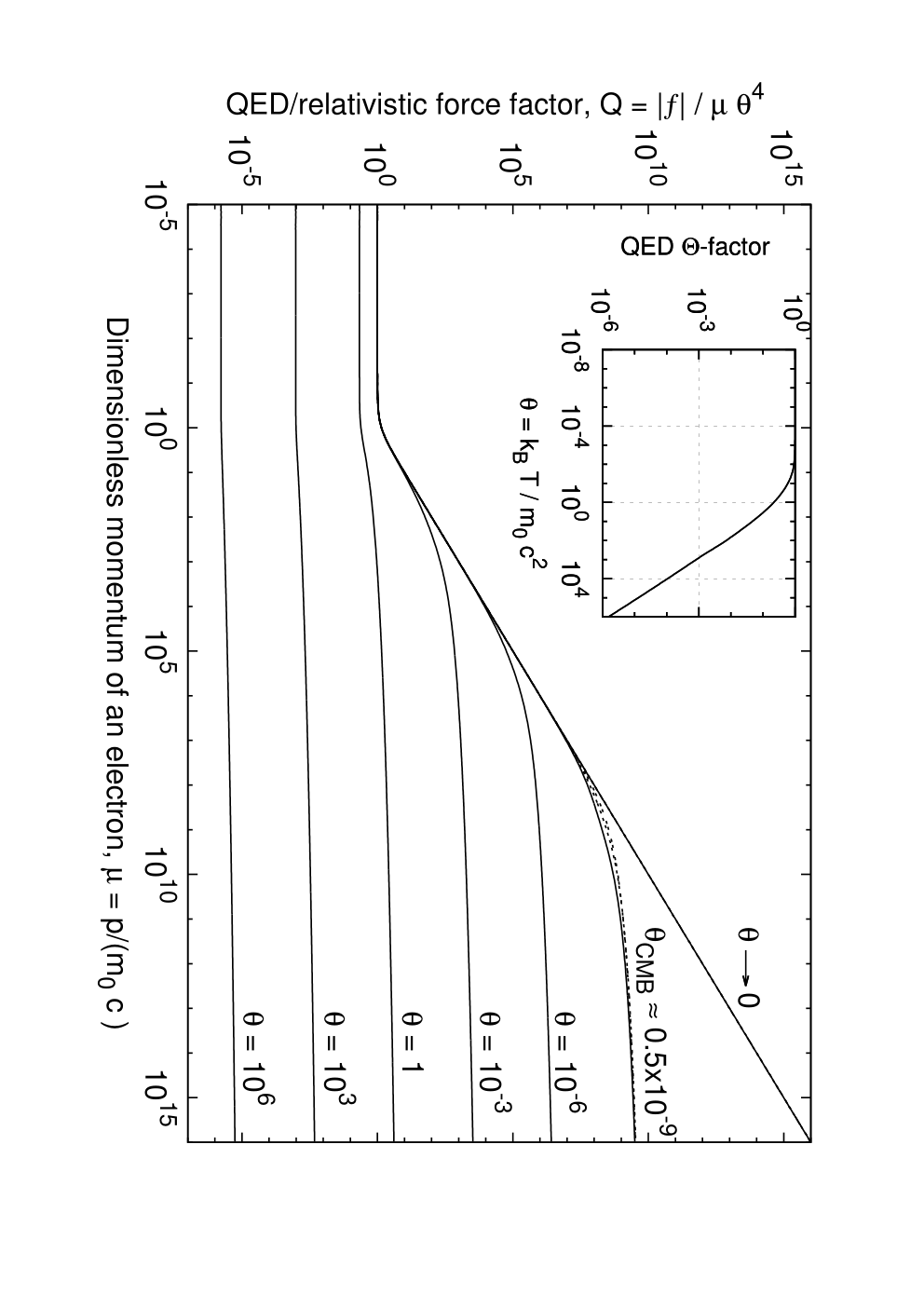
Eqs. (28),(30) together with Eq. (24)-(26) allow for specific investigation of the light pressure by Planck radiation on an electron. The force $f$ $vs$ $\mu$ in the entire momentum span, $\mu\in(0,\mu_{{}_{Pl}})$, and for various $\theta$, from $\theta\sim 10^{-9}$ to $10^{6}$, was numerically evaluated using Eq. (25) and depicted in Fig. 2 for the relativistic/QED factor $Q(\mu,\theta)=-f/\mu\theta^{4}$, where $-\mu\theta^{4}$ is the Thompson non-relativistic light pressure, Eq. (23), for $\gamma=1$; for $\mu,\theta\ll 1$, $Q=1$. In ultra-relativistic QED, or Compton domain, based on the behavior of $\sigma_{{}_{KN}}(\omega)$ at $\omega\rightarrow\infty$, Eq. (28), the asymptotics of $Q$ at $\mu\gg max(1,\theta^{-1})$ can be shown to be $Q\propto[\ln(\theta\mu)+O(1)]/\theta$. Using these numerical and asymptotic results, it would be greatly beneficial for further analysis to have their good analytic interpolation/approximation. Amazingly, this task is perfectly served by a remarkably simple formula good for the entire span $\mu\in(0,\mu_{Pl})$ and $\theta\in(0,\theta_{Pl})$:

where $q=10$ is a fitting parameter. Eq. (31) makes better than a few percents fit to the numerics over the entire span of momentum but a small area near $K_{C}\sim 1$, Fig. 2, where they are still very close; it can be viewed as a benchmark for any other possible approximations. In the limit $K_{C}\ll 1$, Eq. (31) is reduced to Eq. (23). For low-relativistic motion, $\mu\ll 1$, $\gamma\approx 1$, yet arbitrary temperature, the factor $\Theta(\theta)$ in Eq. (26), shown at the inset in Fig. 2, is now approximated using Eq. (31) as

Since $F\equiv dp/dt$, Eq. (15), or $f=d\mu/d\tau$ [see e. g. Eq. (23)], the averaged dynamics of electron motion, $\mu(\tau)$, for $\theta=const$ is implicitly described as $\tau=\int d\mu/f(\mu,\theta)$. It is readily integrated in the case of Thompson scattering, $K_{C}\ll 1$ yielding an explicit function $\mu(\tau)$, Eq. (24), whereas in general case, especially for the transition from Compton domain, $K_{C}\gg 1$ to the Thompson domain, the timeline becomes more complicated, yet still analytically solvable using another approximate model, which is very close to the Eq. (31) in the energy span covering the entire Compton and most of the Thompson domains [41]. In the context of this paper, an important issue is the relaxation time $\tau_{rlx}$ (or rate $\tau_{rlx}^{-1}$) $vs$ temperature $T$ of the electron distribution to its equilibrium state at a given $T$, and the momentum $\mu$ of a non-equilibrium electron. This problem is best handled by using a Fokker-Planck equation for the diffusion in the momentum space [46]. To that end, we consider a distribution function, $g^{(e)}(\mu,\tau)$ of electrons defined here as the number of electrons per element of solid angle $dO$, element of momentum, $d\mu$, within a unity of coordinate space, and a density number, $\rho^{(e)}(\mu,\tau)=$ $4\pi\mu^{2}$ $g^{(e)}$. Note that in application to cosmology, whereby one needs to consider the expanding space/universe, these functions reflect the distribution within the $expanding$ unity of coordinate space, i. e. in the spatial “unity box” expanding at the same rate as the Universe. Assuming then that (a) the electron distribution is isotropic, same as CMB, (b) the total number of electrons, in the unity of momentum space and the expanding unity of coordinate space is approximately invariant, $\int_{0}^{\infty}\rho^{(e)}d\mu=N_{\Sigma}=inv$, and (c) the thermal equilibrium of a relativistic gas at any $\theta$ is due to the Maxwell-Jüttner (MJ) distribution [47,48],

where $K_{2}$ is the modified Bessel function of the second order, with MJ being a relativistic generalization of the Maxwell-Boltzmann distribution,

we found a Fokker-Planck equation for the distribution function $g^{(e)}(\mu,\tau)$, in terms of dimensionless momentum $\mu$, factor $\gamma$, time $\tau$, temperature $\theta$, and force $f$, as

This equation is valid for time-dependant $\theta$ and for the expanding universe For our purposes here we will consider only the case $\theta=const=\theta_{eq}$ (and neglect the universe expansion), since the time involved is mush shorter than the age of universe for the effects of interest here. Eq. (35) is solved fully analytically for the non-relativistic case, $\mu\ll 1$, whereby any initial distribution function $g^{(e)}(\tau=0)$ is decomposed into Gaussian components, Eq. (34), each of which has its specific initial temperature, $\theta_{in}^{(e)}$ at $\tau=0$; in time, their distribution functions remain Gaussian, with their time-dependant effective temperature being as:

i. e. $t_{rlx}=t_{TR}/2=t_{C}/2\theta_{eq}^{4}$ (see eq. (24) and explanations therein). Eq. (36) still holds approximately for the entire Thompson domain for initial conditions close to the equilibrium (be reminded that the condition $K_{C}\ll 1$ automatically means $\theta_{eq}\ll 1$, while proximity to the equilibrium – that $\gamma_{in}=O(1)$ ). In general case of arbitrary initial conditions the relaxation rate becomes

References

- [1] M. Planck, Ann. d. Physik , 69-122 (1900).
- [2] P. Lebedev, Ann. d. Physik, , 433 (1901).
- [3] E. F. Nichols and G. F. Hull, Astroph. J., , 315 and 352 (1903).
- [4] P. Debye, Ann. d. Physik, , 57 (1909).
- [5] L. D. Landau and E. M. Lifshitz, “The Classical Theory of Fields”, Sect. 78, p. 219, 3-th Revised English Edition, Pergamon Press, Oxford, 1971 (translation of 1967 Russian edition, “The Theory of Field”).
- [6] A. Ashkin, Phys. Rev. Lett. , 156 (1970); also in Science, , 1081 (1981).
- [7] T.W. Hänsch and A. L. Schawlow, Opt. Commun. , 68 (1975).
- [8] “Laser Manipulation of Atoms and Ions” Eds. E. Arimondo, W.D. Phillips, and S. Strumina, North-Holland, 1992.
- [9] G. Grynberg and C. Robilliard, Phys. Rep. , 335 (2001).
- [10] A. E. Kaplan, Opt. Express, , 10035 (2009).
- [11] K. Vahala, M. Herrmann, S. Knünz, V. Batteiger, G. Saathoff, T. W. Hänsch, and T. Udem, Nature Phys., , 682 (2009).
- [12] H.A.H.Boot and R.B.R-S.Harvie, Nature , 1187 (1957).
- [13] A.V. Gaponov and M.A. Miller, Soviet Phys. JETP , 168 (1958).
- [14] T.W.B. Kibble, Phys. Rev. Lett. , 1054 (1966).
- [15] P.L. Kapitza and P.A. M. Dirac, Proc. Cambridge Philos. Soc. , 297 (1933).
- [16] M.V. Fedorov, Opt. Commun. , 205 (1974).
- [17] P.H. Bucksbaum, D.W. Schumacher, and M. Bashkansky, Phys. Rev. Lett. , 1182 (1988).
- [18] D.L. Frelmund, K. Aflatoonl and H. Batelan, Nature (London) , 142 (2001).
- [19] A. Ashkin, J. M. Dziedzic, J. E. Bjorkholm, and S. Chu, Opt. Lett. , 288 (1986).
- [20] R.R. Freeman, P.H. Bucksbaum, H. Milchberg, S. Darack, D. Schumacher and M.E. Geusic, Phys. Rev. Lett. ,1092 (1987).
- [21] E. Wells, I. Ben-Itzhak, and R.R. Jones, . , 023001 (2004).
- [22] D. Bauer, P. Mulser, and W.-H. Steeb, Phys. Rev. Lett. , 4622 (1995).
- [23] Z.-M. Sheng, K. Mima, Y.Sentoku, M. S. Jovanovic, T. Taguchi, J. Zhang, and J. Meyer-ter-Vehn, Phys. Rev. Lett. , 055004 (2002).
- [24] A.E. Kaplan and A.L. Pokrovsky, Phys. Rev. Lett. , 053601 (2005).
- [25] A.L. Pokrovsky and A.E. Kaplan, Phys. Rev. , 043401 (2005).
- [26] R. A. Alpher, H. A. Bethe, and G. Gamov, Phys. Rev. , 803 (1948).
- [27] R. A. Alpher and R. C. Herman, Phys. Rev. , 1737 (1948), also in Nature , 774 (1948).
- [28] A. A. Penzias and R. W. Wilson, Astroph. J. , 419 (1965).
- [29] S. Weinberg, ”Cosmology”, Oxford University Press, Oxford, 2008.
- [30] S. Dodelson, “Modern Cosmology”, Academic Press, NY, 2003.
- [31] Y. B. Zel’dovich and I. D. Novikov, ”Relativistic Astrophysics, Vol. 2: The Structure and Evolution of the Universe”, Univ. Chicago Press, Chicago, 1983.
- [32] A. S. Kompaneets, Sov. Phys. JETP , 730 (1957).
- [33] A. F. Illarionov and D. A. Kompaneets, , , 930 (1976).
- [34] Y. B. Zel’dovich and E. V. Levich, JETP Lett. , 35 (1970).
- [35] R. A. Sunyaev and Y. B. Zel’dovich, Astrophys. Space Sci. , 301 (1969); also , 3 (1970), Comm. Astroph. Space Phys. , 173 (1972), and Ann. Rev. Astron. Astrophys. , 537 (1980).
- [36] G. R. Blumenthal and R. J. Gould, Rev. Mod. Phys. , 217 (1970).
- [37] G. B. Rybicki and A. P. Lightman “Radiative Processes in Astrophysics”, Wiley, New York, 1979.
- [38] V.S. Berezinskii, S.V. Bulanov, V.A. Dogiel, V.L. Ginzburg (Ed.), and V.S. Ptuskin, “Astrophysics of Cosmic Rays”, North-Holland, Amsterdam (1990).
- [39] O. Klein and Y. Nishina, Z. Phys. , 853 (1929).
- [40] V.B. Beresteckii, E.M. Livshitz, and L.P. Pitaevskii, “Quantum Electrodynamics”, 2-nd ed., Pergamon, Oxford, 1982. Sect. 86, Eq. (86.16), p. 358.
- [41] A. E. Kaplan, to be published elsewhere.
- [42]
A. E. Kaplan, in “Einstein Collection. 1973,”
Ed. V. L. Ginzburg, publ. by “Nauka”,
Moscow, 1974, p. 396-400,
the Russian original is available at:
http://psi.ece.jhu.edu/~kaplan/PUBL/E.pdf - [43] L.D. Landau and E.M. Lifshitz, ”The Classical Theory of Fields”, 4-th Revised English Edition, Butterworth, Oxford, 1987, Sect. 10, p.31.
- [44] L. D. Landau and E. M. Lifshitz, “Fluid Mechanics”, Sects. 20 & 45, 2-nd ed., Pergamon Press, Oxfordi, 1987.
- [45] L. Lewin, “Dilogarithms and associated functions”. Macdonald, London, 1958. Dilogarithm (Spence) function is available in most of standard numeric math-packages.
- [46] E.M. Lifshitz and L. P. Pitaevskii, ”Physical Kinetics”, Pergamon Press, Oxford, 1981.
- [47] F. Jüttner, Ann. Physik, , 856-882 (1911).
- [48] J. L. Synge, “The Relativistic Gas”, North-Holland, 1957.
- [49] S. Atzeni and J. Meyer-ter-Vehn, ”The Physics of Inertial Fusion”, Oxford University Press, 2004
- [50] M. Tabak, D. S. Clark, S. P. Hatchett, M. H. Key, B. F. Lasinski, R. A. Snavely, S. C. Wilks, R. P. J. Town, R. Stephens, E. M. Campbell, R. Kodama, K. Mima, K. A. Tanaka, S. Atzeni, and R. Freeman, Phys. Plasmas , 057305 (2005).