Mortality Models based on the Transform $\log(-\log x)$

We aim to model curves like those presented in Figure 3. For this purpose, given the non-linear nature of the differences of $L(S(x))$, we borrow representations of mortality like those of James and Segal in [16] or Cairns et al. in [7] and use them to describe such differences. The structures of the methods of these authors are ease to implement and to interpret. In this paper we adopt the representation given by Cairns et al. and allow greater flexibility to age-parameters. Our model, which we called the SL model, for representing and forecasting mortality is, given $x_{0}$, $x_{\min}=x_{0}$, $x_{\max}$, $t_{0}$, and $t_{\min}=t_{0}+1$,

where $\kappa_{x}$ are age-specific constants and, $\alpha_{1,t}$ and $\alpha_{2,t}$ are stochastic processes that are assumed to be measurable at time $t$. Note that $\kappa_{x}$ varies linearly in [7], but in (4) it could vary non-linearly.

To project $L(S_{t}(x))-L(S_{t_{0}}(x))$, we adopt for the two-dimensional time series $\boldsymbol{\alpha}_{t}=(\alpha_{1,t},\alpha_{2,t})^{\prime}$ the dynamics given for the two-dimensional stochastic parameter vector from the CBD model [7], i.e. $\boldsymbol{\alpha}_{t}$ is modeled by the following two-dimensional random walk with drift:

where $\mathbf{a}$ is a constant $2\times 1$ vector, $\mathbf{A}$ is a deterministic $2\times 2$ upper triangular matrix, and $\mathbf{Z}_{t}$ is a two-dimensional standard normal random variable.

Note that from projections of $L(S_{t}(x))-L(S_{t_{0}}(x))$ one can easily compute any mortality variable using the relationships given in Section 2, say for instance survival probabilities, $q_{x,t}$, and $m_{x,t}$.

Next, vaying $t_{0}$ we get extensions of (4), i.e. $t_{0}$ can be considered as another parameter more in (4) and also $x_{0}$. Note that, fixing $t_{\min}$, $t_{0}$ can be chosen smaller than $t_{\min}-1$. Some of these features will be analyzed and exploited in the applications to be presented later.

Let us see numerical illustrations of $L(S_{t}(x))-L(S_{t_{0}}(x))$ when $t_{0}$ varies. Figure 4 shows curves like those exhibited in Figure 3 for French females but now for $t_{0}$ = 1951, 1952, 1953, and 1954. Note that if $t_{0}$ reaches 1955, then the curve corresponding to $t=1955$ does not have interest in the analysis. These new curves are lightly different among them, and it seems that all of them move upward when $t_{0}$ increases.

The corresponding curves of Figure 4 for French males are presented in Figure 5. They are a bit different from the French female curves. Now the lower curves hold concave shapes, but the upper curves are not always concave and present convex pieces.

The model (4), given $t_{0}$ and $x_{0}$, is fitted to computed values of $L(S_{t}(x))-L(S_{t_{0}}(x))$ using ordinary least squares (OLS). It consists in to minimize

As noticed by Brouhns et al. [6], models like (4) are not simple regression models since there are no observed covariates in the right-hand side. Hence alternative ways to find values of $\alpha_{1,t}$, $\alpha_{2,t}$, and $\kappa_{x}$ minimizing (6) are required. We notice that the uni-dimensional or elementary Newton method proposed by Goodman [12] can be used in this case. This method works like the iterative Newton method but considering in each iteration one parameter at a time. In this way each parameter is updated in the iteration $k$ before the iteration of the next parameter in the same iteration $k$. Iteration moves from $k$ to $k+1$ when all the parameters have iterated in the iteration $k$. This process continues until to find the convergence of the sequence of parameter estimates or another stopping condition.

The fitting of (4) to data showed that some parameters may require slow convergences. It was implemented by reducing the variations among iterations, for instance multiplying such variations by a factor $\gamma<1$. This is taken into account in the following iteration algorithm designed to minimize (6):

1. 1.

   Initializations:

   1. (a)

      Initialization of $\alpha_{1,t}$, $\alpha_{2,t}$, and $\kappa_{x}$: $\hat{\alpha}_{1,t}^{(0)}$, $\hat{\alpha}_{2,t}^{(0)}$, and $\hat{\kappa}_{x}^{(0)}$.

      A strategy to obtain these initial values is to fix $\kappa_{x}$ using a known function of $x$. Then one can find estimates $\hat{\alpha}_{1,t}$ and $\hat{\alpha}_{2,t}$ applying linear regressions of $L\big({S}_{t}(x)\big)-L\big({S}_{t_{0}}(x)\big)$ on $\kappa_{x}$ for each $t$.

   2. (b)

      Set the maximal number of iterations $k_{\max}$.

   3. (c)

      Set $k=1$.

2. 2.

   While not convergent and $k<k_{\max}$ do:

   1. (a)

      For $k$ do:

      $\displaystyle\hat{\alpha}_{1,t}^{(k)}=\hat{\alpha}_{1,t}^{(k-1)}+\gamma\sum_{t}\left(L\left({S}_{t}(x)\right)-L\left({S}_{t_{0}}(x)\right)-\hat{\alpha}_{1,t}^{(k-1)}-\hat{\alpha}_{2,t}^{(k-1)}\hat{\kappa}_{x}^{(k-1)}\right)$;

      $\displaystyle\hat{\alpha}_{2,t}^{(k)}=\hat{\alpha}_{2,t}^{(k-1)}+\gamma\frac{\sum_{t}\hat{\kappa}_{x}^{(k-1)}\left(L\left({S}_{t}(x)\right)-L\left({S}_{t_{0}}(x)\right)-\hat{\alpha}_{1,t}^{(k)}-\hat{\alpha}_{2,t}^{(k-1)}\hat{\kappa}_{x}^{(k-1)}\right)}{\sum_{t}\left(\hat{\kappa}_{x}^{(k-1)}\right)^{2}}$; and,

      $\displaystyle\hat{\kappa}_{x}^{(k)}=\hat{\kappa}_{x}^{(k-1)}+\gamma\frac{\sum_{x}\hat{\alpha}_{2,t}^{(k)}\left(L\left({S}_{t}(x)\right)-L\left({S}_{t_{0}}(x)\right)-\hat{\alpha}_{1,t}^{(k)}-\hat{\alpha}_{2,t}^{(k)}\hat{\kappa}_{x}^{(k-1)}\right)}{\sum_{x}\left(\hat{\alpha}_{2,t}^{(k)}\right)^{2}}$.

   2. (b)

      $k=k+1$.

The criterion of convergence is to reach $\big|\hat{v}^{(k)}-\hat{v}^{(k-1)}\big|<\epsilon$, being $v$ any of $\alpha_{1,t}$, $\alpha_{2,t}$, or $\kappa_{x}$, for a reasonably small value of $\epsilon$. When this stopping criterion is satisfied, the OLS estimates of $\alpha_{1,t}$, $\alpha_{2,t}$, and $\kappa_{x}$ using Newton’s method, $\hat{\alpha}_{1,t}$, $\hat{\alpha}_{2,t}$, and $\hat{\kappa}_{x}$, are the final iterative estimates $\hat{\alpha}^{(k)}_{1,t}$, $\hat{\alpha}^{(k)}_{2,t}$, and $\hat{\kappa}^{(k)}_{x}$. In applications to be presented later $\epsilon=10^{-8}$. On $k_{\max}$, the maximal number of iterations, we will fix it in 5,000.

In this paper we use sex-based mortality data from populations of Belgium (BE), France (FR), Italy (IT), Japan (JP), Sweden (SW), United Kingdom (UK), and United States (US). Data, obtained from Human Mortality Database (HMD) [13], correspond to ages from 60 to 94, and to years from 1960 to 2009. No adjustment is made to the data.

A typical dataset consists of the observed variable ${D}_{x,t}$ and the computed variable ${E}_{x,t}$ over the above-mentioned ranges of ages and years. ${D}_{x,t}$ is the number of deaths during calendar year $t$ aged $x$ last birthday and ${E}_{x,t}$ represents an estimated average, during calendar year $t$, of the number of people alive who were aged $x$ last birthday.

With these variables $m_{x,t}$ is estimated by (see e.g. [27])

and $q_{x,t}$ and $S_{t}(x)$ can then be computed using the relationships presented in previous Section. Recall that $S_{t}(x)$ is involved in the LS model, and we will see that $m_{x,t}$ and $q_{x,t}$ are taken into account in the LC and CBD models.

We compare mortality projections of the SL model with those of the LC and CBD models. These two last models are taken as benchmark models since they are well-known and extensively used. Brief descriptions of these models follow.

In this subsection we compare the in-sample and out-of-sample predictive abilities of the LS, LC, and CBD models with respect to data of sex-based $q_{x,t}$ of seven countries. We examine this mortality variable since it is commonly used in practice, for instance to build mortality tables and to compute annuities.

We focus on mortality at higher ages because it is related to population ageing. Age periods from $x_{\min}$ to $x_{\max}$ are analyzed taking $x_{\min}$ = 60, 65 and $x_{\max}$ = 89, 94.

Observed mortality from 1960 to 2009 is used to evaluate in-sample and out-of-sample mortality projection accuracies. This year period is divided in two, the first, from $t_{\min}$ = 1960 to $t_{\max}$ = 1989, to fit the models to data and the second, from 1990 to 2009, to forecast mortality. For the LS model we fix $t_{0}=t_{\min}-1$ in (4).

We examine both in-sample and out-of-sample projection accuracies of $q_{x,t}$ employing a couple of goodness-of-fit criteria often used to evaluate projection performance (see e.g. [18] and [9]). The first criterion is the mean squared error (MSE) defined as

where $X_{i}$ and $\hat{X}_{i}$ are the observed and estimated values of mortality in fitting or forecasting samples, and the second criterion is the mean absolute percentage error (MAPE) defined as

A smaller MSE or MAPE value indicates a better fit to the data on a given period. However, the lowest values of these indexes are not associated to the same model necessarily. We will come back on this issue later.

For each combination of the values of $x_{\min}$ and $x_{\max}$ mentioned above, we present values of MSE and MAPE in Tables 1, 2, 3, and 4. Each of these tables displays countries in rows and sex categories in columns. For each country, the CBD, LC, and LS models are nested. Values of MSE and MAPE are shown for fitting and forecasting year periods, nested in each category of sex. Additionally, in each combination of country and sex and fitting / forecasting year period, the lowest values of MSE and MAPE among the models studied are highlighted, which allow the identification of the models with the best fits. Besides, the values of MSE are displayed with two decimals and those of MAPE with one decimal, this may produce some confusion if a highlighted value equals other values, but there is no conflict since such selection was done using more decimals than those displayed.

A general finding through all these tables is that, as expected, the values of MSE or MAPE on forecasting periods are always much higher than their corresponding values on fitting periods. Also, as indicated above, for fitting as well as for forecasting periods, not always the model with the highest value of MSE is the model with the highest value of MAPE. Additionally, the distributions of the highlighted models are frequently different from a table to another, but in a few cases, for a pair of tables and a given country, one can find the same selection of models. Another finding is that the values of MSE or MAPE, over fitting or forecasting periods, are in general higher for males than for females, which suggests that the modelization of mortality is more difficult for males than for females.

On the fitting period, for females, the highlighted values are concentrated mainly on the LC model and a few cases on the LS model, and none of these values is associated to the CBD model. An interesting feature of the LC model is that it is highlighted almost everywhere when $x_{\max}$ is 94. Regarding males, the highlighted models are concentrated mainly on the CBD and LC models and a few cases on the LS model. Moreover, no model is predominant through all values of $x_{\min}$ and $x_{\max}$.

On the forecasting period, a first observation is that not always the best model over the fitting period corresponds to the best model over the forecasting period. This implies that the distribution of the highlighted values varies between these two periods. On females, we have a sharp presence of the SL model, excepting the case $x_{\min}$ = 60 and $x_{\max}$ = 94. It performs better than the benchmark models for US and UK, and gives the best mortality projection accuracies for JP and SW when $x_{\min}$ = 65 and $x_{\max}$ is 89 or 94. Highlighted values associated to the LC and CDB models appear in a few times. On males, there is a strong presence of the CBD model for an important number of countries through all values of $x_{\min}$ and $x_{\max}$, mainly BE, NE, SW, and US. The LC and SL models are found in a few cases. Nevertheless the scarce selection of the SL model as one of the best models for males, it gives the best mortality projection accuracies for UK for any value of $x_{\min}$ or $x_{\max}$.

The values of MSE and MAPE allow the identification of the best model among the LC, CBD, and LS models, but without any assessment on how well these models fit, i.e. is any of these models acceptable? For answering this question, we focus, for a given age $x$, on the rate of mortality improvement (MI) over the forecasting year period. This rate indicates how mortality rates change with respect to mortality rates of a particular group at a specific point in time.

Rates of MI are often applied to initial mortality levels to establish generational tables to obtain mortality estimates at any future point in time (see e.g. [20]). These rates are also analyzed in function of economical and medical factors to explore their dynamics (see e.g. [25]). In this paper rates of MI are used to assess the performance of the models.

The definition of the rate of MI is not unique (see e.g. [1] and [26]). These rates may be computed as arithmetic or logarithmic rates, they may be based on $q_{x,t}$ or on $m_{x,t}$, and they may be calculated with respect to a given year or to a previous year. We compute annual logarithmic rates of MI with respect to 1989 by, for $x=65$ and considering $x_{\min}=65$ and $x_{\max}=94$, for $t>1989$,

where ${q}_{65,1989}$ is the value of $q_{65,t}$ observed in 1989. Note that this definition can be seen as the cumulative rate of MI in year $t$ with respect to 1989. This rate is expected to be increasing over the years since in the last decades $q_{x,t}$ has shown downward trends.

Figure 6 shows the observed and projected rates of MI obtained for females and for each country. The corresponding rates for males are presented in Figure 7. Through all these figures the curves have upward trends with variations from one year to the next, which is an empirical evidence of the uncertainty of the rates involved. The dynamics of these curves are related to the main concern of the models applied in this article: each time that the curves of projected and observed rates are more separated, the model risk may be higher. In the worst cases the distances between those curves may be systematic and increasing.

On females, Figure 6, the observed rates for IT and US present little variation, and are overlapped by predicted rates given by the CBD and LC models for IT and the LC and SL models for US. On BE, the forecasted rates of the CBD and SL models tend to overlap the observed ones, whereas the forecasted rates of the LC model lightly overestimates the observed ones. For FR, JP, SW, and UK, the observed rates are hard to represent by the benchmark and new models since systematic differences between observed and predicted rates are found.

The behaviors of the forecasted rates for males, Figure 7, are quite different from those for females, Figure 6. On males, we now have through all the countries studied in this paper (excepting JP) that the forecasted rates tend to underestimate the observed rates. The best forecasted rates are found for FR and US, with the LC model for FR and the LS model for US. For the other countries the forecasted rates are away from the observed rates, these differences growing when time increases.

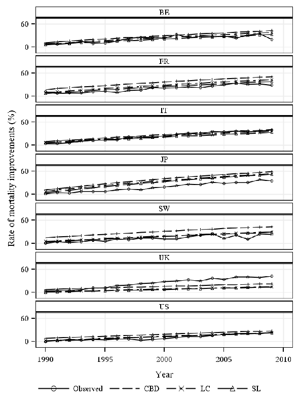
The projected and observed curves shown in Figures 6 and 7 are in general more separated in the last years of the forecasting period. Let us examine the differences among these curves in the two last years, 2008 and 2009, computing the next index of type MAPE.

Results of this index are shown in Table 5. They are organized by country, sex, and $x_{\min}$ and $x_{\max}$, so they contain the cases considered in Figures 6 and 7. The lowest values of $\textrm{MAPE}_{\Delta_{65,2008,2009}}$ among the models studied are highlighted. Smaller highlighted values indicate a better forecast of the data of 2008 and 2009, and a few of them are found only, for instance, considering those near 10.0 % or less, we have IT and US females and FR and US males, all of them representing 21.4 % of the cases. Besides, the SL model seems to be appropriate for mortality forecasting for US females aged 65 and over and for US males aged 60 and over. For US females aged 60 and over the forecasts given by the LS model seem also acceptable.

References

- [1] K. Andreev and J. Vaupel, Patterns of Mortality Improvement over Age and Time in Developed Countries: Estimation, Presentation and Implications for Mortality Forecasting. Paper presented at the Association of America 2005 Annual Meeting program, Philadelphia, Pennsylvania,March 31 - April 2, (2005).
- [2] P. Antolin and H. Blommestein, Governments and the Market for Longevity-Indexed Bonds. OECD Working Papers on Insurance and Private Pensions, (2007).
- [3] H. Booth, R. Hyndman, L. Tickle, and P. de Jong, Lee-Carter mortality forecasting: a multicountry comparison of variants and extensions. Demographic Research 15, (2006) 289-310.
- [4] H. Booth and L. Tickle, Mortality Modelling and Forecasting: a Review of Methods. Annals of Actuarial Science 3, (2008) 3-43.
- [5] W. Brass, Perspectives in Population Prediction: Illustrated by the Statistics of England and Wales. Journal of the Royal Statistical Society. Series A (General) 137, (1974) 532-583.
- [6] N. Brouhns, M. Denuit, and J. Vermunt, A Poisson log-bilinear regression approach to the construction of projected lifetables. Insurance: Mathematics and Economics 31, (2002) 373-393.
- [7] A. Cairns, D. Blake, and K. Dowd, A Two-Factor Model for Stochastic Mortality with Parameter Uncertainty: Theory and Calibration. The Journal of Risk and Insurance 73, (2006) 687-718.
- [8] A. Cairns, D. Blake, K. Dowd, G. Coughlan, D. Epstein, A. Ong, and I. Balevich, A Quantitative Comparison of Stochastic Mortality Models Using Data from England & Wales and the United States. North American Actuarial Journal 13, (2009) 1-35.
- [9] K. Chen, J. Liao, X. Shang, and J. Li, Discussion of “A Quantitative Comparison of Stochastic Mortality Models Using Data from England and Wales and the United States”. North American Actuarial Journal 13, (2009) 514-524.
- [10] P. de Jong and C. Marshall, Mortality projection based on the Wang transform. Astin Bulletin 37, (2007) 149-161.
- [11] A. Deaton and C. Paxson, Mortality, Income, and Income Inequality over Time in Britain and the United States. Perspectives on the Economics of Aging , (2004) 247-285.
- [12] L. Goodman, Simple models for the analysis of association in cross-classifications having ordered categories. Journal of the American Statistical Association 74, (1979) 537-552.
- [13] Human Mortality Database, http://www.mortality.org. (Accessed January 2015). University of California, Berkeley, Max Planck Institute for Demographic Research , (2015).
- [14] R. Hyndman, Booth, L. Tickle, and J. Maindonald, Forecasting mortality, fertility, migration and population data. Package ’demography’. (accessed February 2015) available at http://cran.r-project.org/web/packages/demography/demography.pdf , (2015).
- [15] R. Hyndman and M. Ullah, Robust forecasting of mortality and fertility rates: A functional data approach. Computational Statistics & Data Analysis 51, (2007) 4942-4956.
- [16] I. James and M. Segal, On a Method of Mortality Analysis Incorporating Age-Year Interaction, with Application to Prostate Cancer Mortality. Biometrics 38, (1982) 433-443.
- [17] R. Lee and L. Carter, Modeling and Forecasting U. S. Mortality. Journal of the American Statistical Association 87, (1992) 659-671.
- [18] R. Lee and T. Miller, Evaluating the Performance of the Lee-Carter Method for Forecasting Mortality. Demography 38, (2001) 537-549.
- [19] N. Li and R. Lee, Coherent mortality forecasts for a group of populations: An extension of the Lee-Carter method. Demography 42, (2005) 575-594.
- [20] OECD, Mortality Assumptions and Longevity Risk. Implications for pension funds and annuity providers. OECD Publishing (2014).
- [21] E. Pitacco, Survival models in a dynamic context: a survey. Insurance: Mathematics and Economics 35, (2004) 279-298.
- [22] E. Pitacco, M. Denuit, S. Haberman, and A. Olivieri, Modelling Longevity Dynamics for Pensions and Annuity Business. Oxford University Press (2009).
- [23] A. Renshaw and S. Haberman, A cohort-based extension to the Lee-Carter model formortality reduction factors. Insurance: Mathematics and Economics 38, (2006) 556-570.
- [24] S. Richards and I. Currie, Longevity risk and annuity pricing with the Lee-Carter model. British Actuarial Journal 15, (2009) 317-343.
- [25] RMS, Longevity Risk: Setting the Long Term Mortality Improvement Rate. What medical science tells us about future longevity risk. Risk Management Solutions white paper , (2012).
- [26] SOA, Global Mortality Improvement Experience and Projection Techniques. Society of Actuaries (2011).
- [27] J. Wilmoth, K. Andreev, D. Jdanov, and D. Glei, Methods Protocol for the Human Mortality Database. Version 5. Human Mortality Database , (2007).