Calculating broad neutron resonances in a cut-off Woods-Saxon potential
Abstract
In a cut-off Woods-Saxon (CWS) potential with realistic depth -matrix poles being far from the imaginary wave number axis form a sequence where the distances of the consecutive resonances are inversely proportional with the cut-off radius value, which is an unphysical parameter. Other poles lying closer to the imaginary wave number axis might have trajectories with irregular shapes as the depth of the potential increases. Poles being close repel each other, and their repulsion is responsible for the changes of the directions of the corresponding trajectories. The repulsion might cause that certain resonances become antibound and later resonances again when they collide on the imaginary axis. The interaction is extremely sensitive to the cut-off radius value, which is an apparent handicap of the CWS potential.
pacs
21.10.Pc and 25.40.Dn1 Introduction
Gamow shell model (GSM) [1] became a useful tool in analyzing drip line nuclei produced in laboratories with radioactive beam facilities. A most recent analysis of this type is that of the 7Be(p,)8B and the 7Li(n,)8Li reactions in Ref. [2]. The key elements of GSM are the Berggren-ensembles of single particle states. The Berggren-ensemble might include resonant and sometime antibound states beside the bound states and the scattering states along a complex path. The shape of the path determines the set of the -matrix pole states to be included in the ensemble. In order to have smooth contribution from the scattering states the shape of the path should go reasonably far from the poles. Therefore to know, where the poles are located has crucial importance.
The most common phenomenological nuclear potential used is the cut-off Woods-Saxon (CWS) potential. Two handicaps of the CWS potential are that the positions of the broad resonances do depend on the cut-off radius and the pole trajectories also strongly depend on this radius, which is an unphysical parameter. Moreover some of the trajectories show strange circulating shapes [3]. Two of us suggested an alternative potential, the SV potential [4] which goes to zero smoothly at a finite distance. With SV potential the strange circulating shapes are missing, therefore it was conjectured [3] that the circulation is due to the jump of the CWS at the cut-off radius. In spite of of these handicaps the popularity of using CWS potential is still survives, therefore in this work we study further the pole distribution and the pole trajectories in CWS potential.
2 Formalism
Very little is known about the positions of the broad resonances which correspond to poles lying farther from the real energy or wave-number axes. By varying the strength of the potential we can calculate pole trajectories on the complex wave number () plane. The decaying resonances lie in the fourth quadrant of the plane. The capturing resonances are mirror images of the decaying resonances in a real potential, therefore their trajectories are simply reflected to the imaginary -axis. The complex wave number of a Gamow resonance is with , and for a decaying resonance, and for a capturing resonance. The energy is proportional to , therefore the unbound poles lie on the second energy-sheet. Resonances lying close to the imaginary -axis, when , i.e. , are called as sub-threshold resonances [5]. We want to calculate poles of the -matrix in a given partial wave having orbital angular momentum . The partial wave solution satisfies the radial Schroedinger equation
| (1) |
where prime denotes the derivative with respect to (wrt) the radial distance . The function
| (2) |
is the so called squared local wave number.
In this work we consider a very simple case in which a spin-less neutral particle is scattered on a spherically symmetric target nucleus represented by a real CWS type nuclear potential . The first boundary condition (BC) for the solution is its regularity at :
| (3) |
The other BC is specified at large distance in the asymptotic region, at , i.e. beyond the cut-off radius , where
| (4) |
For a scattering state the asymptotic BC requires that the solution should be a combination of the incoming and outgoing free waves satisfying the Ricatti-Hankel differential equation:
| (5) |
Here is the element of the scattering matrix in the -th partial wave.
For the CWS potential the radial equation in Eq. (1) can be solved only numerically. At the numerical solution should match to that of the asymptotic equation in Eq. (5). We can calculate from the logarithmic derivative at :
| (6) |
were is the internal solution, which is regular at .
The value of the -matrix at a given wave number can be calculated as:
| (7) |
where bar denotes derivative wrt the argument .
3 Resonances as poles of the -matrix
For a resonance the asymptotic BC is defined differently. It is required that the solution and its derivative should be outgoing type and the logarithmic derivative of the external solution is
| (8) |
Both BC (in Eqs. (3) and (8)) can be satisfied simultaneously only at discrete complex eigenvalues, at the poles of . Here the complex eigenvalue is fixed by the zeros of the difference of the logarithmic derivatives of the internal and the external solutions
| (9) |
The computer programs GAMOW [6], and ANTI [7] find the zeros of , at certain matching radius . For a broad resonance the proper choice of this is difficult. The zero is searched by Newton iterations, and the iteration process often converges poorly or fails. Therefore we developed a new method in which we compare the logarithmic derivatives in a wide region in . This method is built into the program JOZSO11 1 The program name is chosen to honor the late József Zimányi to whom one of the authors (T. Vertse) is grateful for starting his carrier. [8]. We calculate in Eq. (9) at equidistant mesh-points with mesh size at , . The mesh points are taken from a region where the nuclear potential falls most rapidly. Then we search for the absolute minimum of the function of two real variables , and :
| (10) |
Absolute minima of the function in Eq. (10) should have a large negative value. The position of the absolute minimum is the pole position of . The minimum of the function is found by using the Powell’s method in Ref. [9]. To find the minima of the function first we explore the landscape of the function in a complex domain of our interest. We plot the function , which has peaks at the poles of on a grid (see e.g. Fig. 1).
4 Pole trajectories in CWS potential
The nuclear potential in Eq. (2) is in fm-2 units, like the is. It is more usual however, to give it the same units in which the energy is given, i.e. in MeV. It is also usual to give the potential as a product of its strength in MeV and its dimensionless radial shape:
| (11) |
where the later is
| (12) |
Here denotes the Heaviside step function, being zero for negative and unity for non-negative arguments. The parameters of the shape in Eq. (12) are the radius , the diffuseness and the cut-off radius .
Sometimes it is useful to draw the trajectories of the individual poles, i.e. to explore how the positions of the poles change when we keep the shape of the CWS potential fixed but vary the strength of the potential. By increasing the pole trajectory moves to the upper half of the -plane, where it becomes a bound state with negative real energy and with purely imaginary . Here the solution becomes a real function with finite number of zeros. The nodes number counts the zeros of the bound state wave function outside .
Antibound solutions belong to poles of on the negative wing of the imaginary -axis. They diverge without oscillations in the asymptotic region as . The poles of the lying off the imaginary -axis on the lower half of the -plane are resonances. For a resonance the wave function is complex and the tail of the wave function (in both the real and the imaginary parts) oscillates around -axis with exponentially growing amplitude as . Both parts have infinite number of zeros.
5 Numerical example
Here we study the positions of the poles for , where we have a centrifugal barrier. Among the resonances we have poles with small imaginary parts. These narrow resonances appear only if we have a barrier in the potential. As example we calculate the neutron single-particle resonances in the 208Pb system in the CWS potential used in Ref. [12] but without the spin-orbit term. The values of the potential parameters are: MeV, , , . Here we present only results, which show a typical example for the cases.

In Fig. 1 we present the surface calculated for fm for CWS potential. The peaks of the surface show the approximate pole positions of the resonances. They give only a hint for the location of the poles, and help us to give reasonably good starting values for finding the poles of more accurately, when we calculate the minima of the quantity in Eq. (10) for each pole. The positions of the three lowest lying poles in the domain , and are listed in Table 1. Decaying resonances are denoted by with , and capturing ones by with . We assign a sequence number to the poles as their value increase.
| 1 | 0.076 | -0.147 | 4 |
| 2 | 0.438 | -0.603 | 3 |
| 3 | 0.752 | -0.449 | 5 |
Note that the node number in the fourth column does not increase monotonously with in the first column. Observe also that the poles with and are sub-threshold resonances.
In the left corner of the landscape one can see a tiny pair of poles. They are the poles in Table 1 (). On the right and middle part of the figure we can see a mountain with almost equidistant peaks.
The resonance is a member of this peak-sequence lying closest to the imaginary axis. Below this pole lies the sub-threshold resonance with considerably larger value than the rest of the peaks forming the mountain.
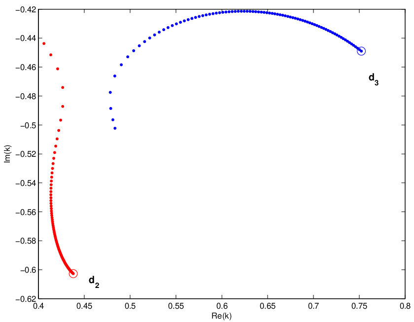
To understand the dynamics of the poles it is very useful to produce an animation (see Ref. [13]) in which the potential depth is changing by in each temporal step and we can see how the landscape changes in a given domain as a function of . In the animation we can conveniently follow the move of the poles as a function of . In Fig. 2 we show the trajectories of the poles with starting positions listed in Table 1. We plot their trajectories in a domain in the third and forth quadrants.

By increasing starting from MeV the pair in Fig. 2 moves downward and the pair upward. The third pair moves toward the imaginary axis and interacts with the second pair . The repulsive interaction between them is shown in a magnified scale in Fig. 3. The and resonances repel each other when they come close at MeV. The repulsion changes the direction of the trajectory slightly towards the imaginary axis, while turns down and move farther from the imaginary axis.
The repulsion produces some sort of avoided crossing of the resonance levels. For narrow resonances similar phenomenon was observed in axially deformed Woods-Saxon potential in Ref. [14] when the deformation was changed. The repulsive interaction is extremely sensitive to the value of . A small change from fm to fm reduced the closest distance between the resonances to half of the distance shown in Fig. 3.
Increasing the value further the pair of poles interacts with the pair and pushes it to the imaginary axis at about . After the collision the pair move upward and the pole collides in the origin with the pole. They form a double pole there. Increasing the strength further the pole becomes to be a bound pole with node number . The other pole what we still call as moves down along the imaginary axis. (In identifying the separating poles from the double pole in the origin, we shifted them a bit from the origin by applying a small imaginary potential strength.) At MeV antibound pole meets the upward moving antibound pole at about on the imaginary axis. After the collision of the two antibound poles they move off the axis, turns left, turns right and they become resonances again. The and resonances move along cucumber like paths symmetrically to the imaginary axis and at the ends of the paths they collide in the origin forming a double pole there. After that the pole becomes to be a bound state pole with node number , and pole starts moving down again along the imaginary axis as an antibound pole. We shall see that the pole plays the role of a bouncer, since it creates bound state poles from the double-poles in the origin.
An unexpected feature of the case is that resonances meet with pole twice and they form double pole twice on the imaginary axis. First when the cucumber-like path starts and the second time when they meet in the origin.
The same pattern is repeated again and again, i.e. the members of the symmetric pair of poles meet on the imaginary axis well below the origin and the member coming from the forth quadrant turns down, the other coming from the third quadrant turns up and collides higher with the bouncer () twice.
6 Summary
As a summary, we can conclude that for CWS potentials the pole positions are sensitive to the value of the cut-off radius and their interaction is extremely sensitive to it. The distance of the poles in the mountain is regulated by the value, as it was observed in Ref. [4] for . The larger the value is, the closer the peaks are to each other. The close lying poles might interact with each other. When the resonances come close to the imaginary axis they might become antibound states and they might interact with other antibound poles moving along the imaginary axis. The interactions between poles distort the pole trajectories. Such distorted trajectories have been observed earlier in Ref. [15] where the starting values of the trajectories were calculated for 18F. (Starting value of the trajectory is, when is very small). In that paper it was observed that the positions of the starting values of the resonances are governed by the value. In Fig. 8. of that reference the trajectory shows a loop. Strange circulating shapes were observed for also in Fig. 1. of Ref. [3] for the pole trajectories of the CWS for different values.
It is reasonable to assume that the repulsive interaction between poles is responsible for all these strange trajectory shapes. Large value of pushes the resonance pole too close to each other, where they interact. To reduce the possibility of this interaction we suggest to use a relatively small value for the cut-off radius not much larger than the range of the best fit SV potential.
Acknowledgement
Authors are grateful to I. Hornyák for valuable discussions. This work was supported by the OTKA Grant No. K112962.
References
- (1) N. Michel, W. Nazarewicz, M. Płoszajczak, and T. Vertse, J. Phys. G. 36, 013101 (2009).
- (2) K. Fossez, N. Michel, M. Płoszajczak, Y. Jaganathen, and R. M. Id Betan, Phys. Rev. C 91, 034609 (2015).
- (3) T. Vertse, R. G. Lovas, P. Salamon, and A. Rácz, AIP Conf. Proc. 1491, 113 (2012).
- (4) P. Salamon and T. Vertse, Phys. Rev. C 77, 037302 (2008).
- (5) A. M. Mukhamedzhanov, B. F. Irgaziev, V. Z. Goldberg, Yu. V. Orlov, and I. Qazi, Phys. Rev. C 81, 054314 (2010).
- (6) T. Vertse, K. F. Pál, Z. Balogh, Computer Physics Communications 27, 309 (1982).
- (7) L.Gr. Ixaru, M. Rizea, T. Vertse, Computer Physics Communications 85, 217 (1995).
- (8) Cs. Noszály, Á. Baran, P. Salamon, and T. Vertse, JOZSO, a renewed version of the computer code GAMOW for calculating broad neutron resonances in phenomenological nuclear potentials, to be submitted to Computer Physics Communications.
- (9) W. H. Press, B. P. Flannery, S. A. Teukolsky, W. T. Vetterling, Numerical Recipes, Cambridge University Press, Cambridge, 1987.
- (10) J. Darai, A. Rácz, P. Salamon, and R. G. Lovas, Phys. Rev. C 86, 014314 (2012).
- (11) A. Rácz, P. Salamon, and T. Vertse, Phys. Rev. C 84, 037602 (2011).
- (12) P. Curutchet, T. Vertse, and R. J. Liotta, Phys. Rev. C 39, 1020 (1989).
- (13) www.atomki.hu/atomki/TheorPhys/TrajAnimL2R15.avi
- (14) L. S. Ferreira, E. Maglione, and R. J. Liotta, Phys. Rev. Lett. 78, 1640 (1997).
- (15) P. Salamon, R. G. Lovas, R. M. Id Betan, T. Vertse, and L. Balkay, Phys. Rev. C 89, 054609 (2014).
Published in Eur. Phys. J. A (2015) 51: 76.
DOI 10.1140/epja/i2015-15076-1