跳到论文正文
W Papers独立论文阅读器 arXiv:1502.07108 论文正文 计算阅读时间 · 0%
引用这篇论文根据当前论文元数据生成,正式投稿前建议核对。


License: arXiv.org perpetual non-exclusive license
arXiv:1502.07108v1 [hep-ph] 25 Feb 2015

Parton distributions at low xx and gluon- and quark average multiplicities

Abstract: 

We shown the general approach for Q2Q^{2} evolution of parton densities and fragmentation functions at low xx based on the diagonalization. The diagonalization leads to the two components in the Q2Q^{2} evolution, each of which contains a nonperturbative parameter. The values of the parameters can be found by fits of the experimental data for the deep-inelastic scattering structure function F2F_{2} and for average jet multiplicities. One of the components contains the all large logarithms ln⁡(1/x)\ln(1/x) and produce the basic contribution at small xx region. The second one is regular at low xx but its contribution is very important to have a good agreement with experimental data.

††conference: XXII International Baldin Seminar on High Energy Physics Problems,
15-20 September 2014
JINR, Dubna, Russia

1 Introduction

The evaluation of the cross-sections for hadron-hadron iteractions needs the sufficiently precise knowledge of parton distribution functions (PDFs) and parton fragmentation functions (FFs), which are the important part of any cross-section. The properties of PDFs and FFs can be taken from processes of the deep-inelatic scattering (DIS) and e+​e−e^{+}e^{-}-collisions, respectively. In this report we will concentrate only for the high-energy limits of PDFs and FFs, which are needed for modern experiments studied on LHC collider.

1.1 PDFs

The experimental data from HERA on the DIS structure function (SF) F2F_{2} [1]-[3], its derivative ∂ln⁡F2/∂ln⁡(1/x)\partial\ln F_{2}/\partial\ln(1/x) [4] and the heavy quark parts F2c​cF_{2}^{cc} and F2b​bF_{2}^{bb} [5] enable us to enter into a very interesting kinematical range for testing the theoretical ideas on the behavior of quarks and gluons carrying a very low fraction of momentum of the proton, the so-called small-xx region. In this limit one expects that the conventional treatment based on the Dokshitzer–Gribov–Lipatov–Altarelli–Parisi (DGLAP) equations [6] does not account for contributions to the cross section which are leading in αs​ln⁡(1/x)\alpha_{s}\ln(1/x) and, moreover, the parton densities are becoming large and need to develop a high density formulation of QCD. However, the reasonable agreement between HERA data and the next-to-leading-order (NLO) and next-to-next-to-leading-order (NNLO) approximations of perturbative QCD has been observed for Q2≥2Q^{2}\geq 2 GeV2 (see reviews in [7] and references therein) and, thus, perturbative QCD could describe the evolution of F2F_{2} and its derivatives up to very low Q2Q^{2} values, traditionally explained by soft processes.

The standard program to study the xx behavior of quarks and gluons is carried out by comparison of data with the numerical solution of the DGLAP equation [6]11 1 At small xx there is another approach based on the Balitsky–Fadin–Kuraev–Lipatov (BFKL) equation [8], whose application is out of the scope of this work. by fitting the parameters of the PDF xx-profile at some initial Q02Q_{0}^{2} and the QCD energy scale Λ\Lambda [9]-[12]. However, for analyzing exclusively the low-xx region, there is the alternative of doing a simpler analysis by using some of the existing analytical solutions of DGLAP evolution in the low-xx limit [13]–[16]. This was done so in [13] where it was pointed out that the HERA small-xx data can be interpreted in terms of the so-called doubled asymptotic scaling (DAS) phenomenon related to the asymptotic behavior of the DGLAP evolution discovered many years ago [17].

The study of [13] was extended in [14, 15, 16] to include the finite parts of anomalous dimensions of Wilson operators 22 2 In the standard DAS approximation [17] only the singular parts of the anomalous dimensions were used.. This has led to predictions [15, 16] of the small-xx asymptotic PDF form in the framework of the DGLAP dynamics starting at some Q02Q^{2}_{0} with the flat function

fa​(Q02)=Aa(hereafter ​a=q,g),\displaystyle f_{a}(Q^{2}_{0})~=~A_{a}~~~~(\mbox{hereafter }a=q,g), (1)

where faf_{a} are the parton distributions multiplied by xx and AaA_{a} are unknown parameters to be determined from the data.

1.2 FFs and average jet multiplicities

Collisions of particles and nuclei at high energies usually produce many hadrons and their production is a typical process where nonperturbative phenomena are involved. However, for particular observables, this problem can be avoided. In particular, the counting of hadrons in a jet that is initiated at a certain scale QQ belongs to this class of observables. Hence, if the scale QQ is large enough, this would in principle allow perturbative QCD to be predictive without the need to consider phenomenological models of hadronization. Nevertheless, such processes are dominated by soft-gluon emissions, and it is a well-known fact that, in such kinematic regions of phase space, fixed-order perturbation theory fails, rendering the usage of resummation techniques indispensable. As we shall see, the computation of average jet multiplicities (AJMs) indeed requires small-xx resummation, as was already realized a long time ago [18]. In Ref. [18], it was shown that the singularities for x∼0x\sim 0, which are encoded in large logarithms of the kind 1/x​lnk⁡(1/x)1/x\ln^{k}(1/x), spoil perturbation theory, and also render integral observables in xx ill-defined, disappear after resummation. Usually, resummation includes the singularities from all orders according to a certain logarithmic accuracy, for which it restores perturbation theory.

Small-xx resummation has recently been carried out for timelike splitting fuctions in the MS¯\overline{\mathrm{MS}} factorization scheme, which is generally preferable to other schemes, yielding fully analytic expressions. In a first step, the next-to-leading-logarithmic (NLL) level of accuracy has been reached [19, 20]. In a second step, this has been pushed to the next-to-next-to-leading-logarithmic (NNLL), and partially even to the next-to-next-to-next-to-leading-logarithmic (N3LL), level [21]. Thanks to these results, we were able in [22, 23] to analytically compute the NNLL contributions to the evolutions of the gluon and quark AJMs with normalization factors evaluated to NLO and approximately to next-to-next-to-next-to-order (N3LO) in the αs\sqrt{\alpha_{s}} expansion. The previous literature contains a NLL result on the small-xx resummation of timelike splitting fuctions obtained in a massive-gluon scheme. Unfortunately, this is unsuitable for the combination with available fixed-order corrections, which are routinely evaluated in the MS¯\overline{\mathrm{MS}} scheme. A general discussion of the scheme choice and dependence in this context may be found in Refs. [24].

The gluon and quark AJMs, which we denote as ⟨nh​(Q2)⟩g\langle n_{h}(Q^{2})\rangle_{g} and ⟨nh​(Q2)⟩q\langle n_{h}(Q^{2})\rangle_{q}, respectively, represent the average numbers of hadrons in a jet initiated by a gluon or a quark at scale QQ. In the past, analytic predictions were obtained by solving the equations for the generating functionals in the modified leading-logarithmic approximation (MLLA) in Ref. [25] through N3LO in the expansion parameter αs\sqrt{\alpha_{s}}, i.e. through 𝒪⁡(αs3/2)\mathcal{O}(\alpha_{s}^{3/2}). However, the theoretical prediction for the ratio r⁡(Q2)=⟨nh​(Q2)⟩g/⟨nh​(Q2)⟩qr(Q^{2})=\langle n_{h}(Q^{2})\rangle_{g}/\langle n_{h}(Q^{2})\rangle_{q} given in Ref. [25] is about 10% higher than the experimental data at the scale of the Z0Z^{0} boson. An alternative approach was proposed in Ref. [26], where a differential equation for the gluon-to-quark AJM ratio was obtained in the MLLA within the framework of the colour-dipole model, and the constant of integration, which is supposed to encode nonperturbative contributions, was fitted to experimental data. A constant offset to the gluon and quark AJMs jet multiplicities was also introduced in Ref. [27].

Recently, we proposed a new formalism [28, 22, 23] that solves the problem of the apparent good convergence of the perturbative series and does not require any ad-hoc offset, once the effects due to the mixing between quarks and gluons are fully included. Our result is a generalization of the result obtained in Ref. [25]. In our new approach, the nonperturbative informations to the gluon-to-quark AJM ratio are encoded in the initial conditions of the evolution equations.

This contribution is organized as follows. Section 2 contains general formulae for the Q2Q^{2}-evolution of PDFs and FFs. The generalized DAS approach is presented in Section 3. Sections 4 and 5 contain basic formulae of Q2Q^{2}-dependence of FFs at low xx and the AJMs, respectively. In Section 6 we compare our formulae with the experimental data for the DIS SF F2F_{2} and the AJMs and present the obtained results. Some discussions can be found in the conclusions. The procedure of the diagonalization and its results for PDF and SF Mellin moments can be found in AppendixA.

2 Approach

Here we breifly touch on some points concerning theoretical part of our analysis.

2.1 Strong coupling constant

The strong coupling constant is determined from the renormalization group equation. Moreover, the perturbative coupling constant as​(Q2)a_{s}(Q^{2}) is different at the leading-order (LO), NLO and NNLO approximations. Indeed, from the renormalization group equation we can obtain the following equations for the coupling constant

1asLO​(Q2)−1asLO​(MZ2)=β0​ln⁡(Q2MZ2)\displaystyle\frac{1}{a_{s}^{\rm LO}(Q^{2})}-\frac{1}{a_{s}^{\rm LO}(M_{Z}^{2})}\,=\,\beta_{0}\ln{\left(\frac{Q^{2}}{M_{Z}^{2}}\right)} (2)

at the LO approximationm and

1asNLO​(Q2)−1asNLO​(MZ2)+b1​ln⁡[asNLO​(Q2)​(1+b1​asNLO​(MZ2))asNLO​(MZ2)​(1+b1​asNLO​(Q2))]=β0​ln⁡(Q2MZ2)\displaystyle\frac{1}{a_{s}^{\rm NLO}(Q^{2})}-\frac{1}{a_{s}^{\rm NLO}(M_{Z}^{2})}\,+\,b_{1}\ln{\left[\frac{a_{s}^{\rm NLO}(Q^{2})(1+b_{1}a_{s}^{\rm NLO}(M_{Z}^{2}))}{a_{s}^{\rm NLO}(M_{Z}^{2})(1+b_{1}a_{s}^{\rm NLO}(Q^{2}))}\right]}\,=\,\beta_{0}\ln{\left(\frac{Q^{2}}{M_{Z}^{2}}\right)} (3)

at the NLO approximation.

At NNLO level asNNLO​(Q2)≡as​(Q2)a_{s}^{\rm NNLO}(Q^{2})\equiv a_{s}(Q^{2}) is more complicated and it is given by

1as​(Q2)−1as​(MZ2)+b1​ln⁡[as​(Q2)as​(MZ2)​1+b1​as​(MZ2)+b2​as2​(MZ2)1+b1​as​(Q2)+b2​as2​(Q2)]+(b2−b122)⋅I=β0​ln⁡(Q2MZ2).\frac{1}{a_{s}(Q^{2})}-\frac{1}{a_{s}(M_{Z}^{2})}+b_{1}\ln{\left[\frac{a_{s}(Q^{2})}{a_{s}(M_{Z}^{2})}\sqrt{\frac{1+b_{1}a_{s}(M_{Z}^{2})+b_{2}a_{s}^{2}(M_{Z}^{2})}{1+b_{1}a_{s}(Q^{2})+b_{2}a_{s}^{2}(Q^{2})}}\right]}+\left(b_{2}-\frac{b_{1}^{2}}{2}\right)\cdot I=\beta_{0}\ln{\left(\frac{Q^{2}}{M_{Z}^{2}}\right)}\,. (4)

The expression for II looks:

I={2Δ​(arctan⁡b1+2​b2​as​(Q2)Δ−arctan⁡b1+2​b2​as​(MZ2)Δ)for f=3,4,5;Δ>0,1−Δ​ln⁡[b1+2​b2​as​(Q2)−−Δb1+2​b2​as​(Q2)+−Δ⋅b1+2​b2​as​(MZ2)+−Δb1+2​b2​as​(MZ2)−−Δ]for f=6;Δ<0,I=\cases{\displaystyle{\frac{2}{\sqrt{\Delta}}}\left(\arctan{\displaystyle{\frac{b_{1}+2b_{2}a_{s}(Q^{2})}{\sqrt{\Delta}}}}-\arctan{\displaystyle{\frac{b_{1}+2b_{2}a_{s}(M_{Z}^{2})}{\sqrt{\Delta}}}}\right)&for $f=3,4,5;\Delta>0$,\cr\displaystyle{\frac{1}{\sqrt{-\Delta}}}\ln{\left[\frac{b_{1}+2b_{2}a_{s}(Q^{2})-\sqrt{-\Delta}}{b_{1}+2b_{2}a_{s}(Q^{2})+\sqrt{-\Delta}}\cdot\frac{b_{1}+2b_{2}a_{s}(M_{Z}^{2})+\sqrt{-\Delta}}{b_{1}+2b_{2}a_{s}(M_{Z}^{2})-\sqrt{-\Delta}}\right]}&for $f=6;\quad\Delta<0$,\cr}

where Δ=4​b2−b12\Delta=4b_{2}-b_{1}^{2} and bi=βi/β0b_{i}=\beta_{i}/\beta_{0} are read off from the QCD β\beta-function:

β⁡(as)=−β0​as2−β1​as3−β2​as4+…=−β0​as2​(1+b1​as+b2​as2+…),\beta(a_{s})~=~-\beta_{0}a_{s}^{2}-\beta_{1}a_{s}^{3}-\beta_{2}a_{s}^{4}+\ldots=-\beta_{0}a_{s}^{2}\Biggl(1+b_{1}a_{s}+b_{2}a_{s}^{2}+\ldots\Biggr)\,, (5)

where

β0=11−23​f,β1=102−383​f,β2=28572−503318​f+32554​f2,\beta_{0}=11-\frac{2}{3}f,~~\beta_{1}=102-\frac{38}{3}f,~~\beta_{2}=\frac{2857}{2}-\frac{5033}{18}f+\frac{325}{54}f^{2}, (6)

with ff being the number of active quark flavours.

2.2 PDFs and DIS SF F2F_{2}

The DIS SF can be represented as a sum of two terms:

F2​(x,Q2)=F2N​S​(x,Q2)+F2S​(x,Q2),F_{2}(x,Q^{2})=F_{2}^{NS}(x,Q^{2})+F_{2}^{S}(x,Q^{2})\,, (7)

the nonsinglet (NS) and singlet (S) parts. At this point let’s introduce PDFs, the gluon distribution function fg​(x,Q2)f_{g}(x,Q^{2}) and the singlet and nonsinglet quark distribution functions fS​(x,Q2)f_{S}(x,Q^{2}) and fN​S​(x,Q2)f_{NS}(x,Q^{2}) 33 3 Unlike the standard case, here PDFs are multiplied by xx.:

𝐟S​(x,Q2)\displaystyle{\bf f}_{S}(x,Q^{2}) ≡\displaystyle\equiv ∑if𝐟i​(x,Q2)=V⁡(x,Q2)+S⁡(x,Q2),\displaystyle\sum_{i}^{f}{\bf f}_{i}(x,Q^{2})=V(x,Q^{2})+S(x,Q^{2})\,,
𝐟N​S​(x,Q2)\displaystyle{\bf f}_{NS}(x,Q^{2}) ≡\displaystyle\equiv ∑ifei2​𝐟iN​S​(x,Q2),𝐟iN​S​(x,Q2)=𝐟i​(x,Q2)−1f​𝐟S​(x,Q2),\displaystyle\sum_{i}^{f}e^{2}_{i}\,{\bf f}^{NS}_{i}(x,Q^{2}),~~{\bf f}^{NS}_{i}(x,Q^{2})={\bf f}_{i}(x,Q^{2})-\frac{1}{f}\,{\bf f}_{S}(x,Q^{2})\,, (8)

where V⁡(x,Q2)=𝐮v​(x,Q2)+𝐝v​(x,Q2)V(x,Q^{2})={\bf u}_{v}(x,Q^{2})+{\bf d}_{v}(x,Q^{2}) is the distribution of valence quarks and S⁡(x,Q2)S(x,Q^{2}) is a sum of sea parton distributions set equal to each other.

There is a direct relation between SF moments  Mn​(Q2)M_{n}(Q^{2}) and those of PDFs

Mj(n,Q2)=∫01dxxn−2F2j(x,Q2),𝐟j(n,Q2)=∫01dxxn−2𝐟j(x,Q2),(j=NS,S,G),M^{j}(n,Q^{2})~=~\int_{0}^{1}dxx^{n-2}F^{j}_{2}(x,Q^{2}),~~{\bf f}_{j}(n,Q^{2})~=~\int_{0}^{1}dxx^{n-2}{\bf f}_{j}(x,Q^{2}),~~~(j=NS,S,G), (9)

which has the following form

MnN​S​(Q2)\displaystyle M_{n}^{NS}(Q^{2}) =\displaystyle= CN​S​(n,a¯s​(Q2))⋅𝐟N​S​(n,Q2),\displaystyle C_{NS}(n,\overline{a}_{s}(Q^{2}))\cdot{\bf f}_{NS}(n,Q^{2})\,, (10)
MnS​(Q2)\displaystyle M_{n}^{S}(Q^{2}) =\displaystyle= e⁡(CS​(n,a¯s​(Q2))⋅𝐟S​(n,Q2)+Cg​(n,a¯s​(Q2))⋅𝐟G​(n,Q2)),\displaystyle e\,\biggl(C_{S}(n,\overline{a}_{s}(Q^{2}))\cdot{\bf f}_{S}(n,Q^{2})+C_{g}(n,\overline{a}_{s}(Q^{2}))\cdot{\bf f}_{G}(n,Q^{2})\biggr)\,,~~~~~~ (11)

with Cj​(n,a¯s​(Q2))C_{j}(n,\overline{a}_{s}(Q^{2})) (j=N​S,S,G)(j=NS,S,G) are the Wilson coefficient functions. The constant ee depends on weak and electromagnetic charges and is fixed for electromagnetic charges to

e=1f​∑qfeq2.e~=~\frac{1}{f}\,\sum_{q}^{f}e^{2}_{q}\,. (12)

Note that the NS and valence quark parts are negledgible at low xx and, thus, F2S​(x,Q2)=F2​(x,Q2)F_{2}^{S}(x,Q^{2})=F_{2}(x,Q^{2}) and S⁡(x,Q2)=𝐟S​(n,Q2)≡𝐟q​(n,Q2)S(x,Q^{2})={\bf f}_{S}(n,Q^{2})\equiv{\bf f}_{q}(n,Q^{2}).

2.3 Q2Q^{2}-dependence of SF moments

The coefficient functions Cq​(n,as​(Q2))≡CS​(n,as​(Q2))C_{q}(n,a_{s}(Q^{2}))\equiv C_{S}(n,a_{s}(Q^{2})) and Cg​(n,as​(Q2))C_{g}(n,a_{s}(Q^{2})) are further expressed through the functions Bq(i)​(n)B^{(i)}_{q}(n) and Bg(i)​(n)B^{(i)}_{g}(n), respectively, which are known exactly [29, 30] 44 4 For the integral and even complex nn values, the coefficients Ba(i)​(n)B^{(i)}_{a}(n) and Za,b(i)​(n)Z^{(i)}_{a,b}(n) (a,b=q,g)(a,b=q,g) can be obtained using the analytic continuation [31].

Ca​(n,as​(Q2))=1−δag+as⋅Ba(1)​(n)+as2⋅Ba(2)​(n)+𝒪⁡(as3),(a=(q,g))C_{a}(n,a_{s}(Q^{2}))=1-\delta^{g}_{a}+a_{s}\cdot B^{(1)}_{a}(n)+a_{s}^{2}\cdot B_{a}^{(2)}(n)+{\cal O}(a_{s}^{3})\,,~~~(a=(q,g))\, (13)

where δag\delta^{g}_{a} is the Kroneker symbol.

The Q2Q^{2}-evolution of the PDF moments can be calculated within a framework of perturbative QCD (see e.g. [30, 32]). After diagonalization (see Appendix A), we see that the quark and gluon densities contain the so called "+""+"- and "−""-"-components

𝐟a​(n,Q2)=𝐟a+​(n,Q2)+𝐟a−​(n,Q2)​(a=q,g),{\bf f}_{a}(n,Q^{2})={\bf f}_{a}^{+}(n,Q^{2})+{\bf f}_{a}^{-}(n,Q^{2})~~~(a=q,g), (14)

which in-turn evaluated already independently:

𝐟a±​(n,Q2)=𝐟~a±​(n,Q02)⋅[as​(Q2)as​(Q02)]γ±(0)​(n)2​β0⋅Ha±​(n,Q2),{\bf f}_{a}^{\pm}(n,Q^{2})={\bf\tilde{f}}_{a}^{\pm}(n,Q_{0}^{2})\cdot\left[\frac{a_{s}(Q^{2})}{a_{s}(Q^{2}_{0})}\right]^{\frac{\gamma_{\pm}^{(0)}(n)}{2\beta_{0}}}\cdot H_{a}^{\pm}(n,Q^{2})\,, (15)

where

γ±(0)​(n)=12​(γq​q(0)​(n)+γg​g(0)​(n)±(γq​q(0)​(n)−γg​g(0)​(n))+4​γq​g(0)​(n)​γg​q(0)​(n))\gamma_{\pm}^{(0)}(n)~=~\frac{1}{2}\biggl(\gamma_{qq}^{(0)}(n)+\gamma_{gg}^{(0)}(n)\pm\sqrt{\Bigl(\gamma_{qq}^{(0)}(n)-\gamma_{gg}^{(0)}(n)\Bigr)+4\gamma_{qg}^{(0)}(n)\gamma_{gq}^{(0)}(n)}\biggr) (16)

is the anomalous dimensions of the "+""+"- and "−""-"-components, which are obtained from the elements of the martix of the LO anomalous quark and gluon anomalous dimensions.

At LO, the normalization coefficients 𝐟~a±​(n,Q02){\bf\tilde{f}}_{a}^{\pm}(n,Q_{0}^{2}) have the form

𝐟~a±​(n,Q02)=𝐟a±​(n,Q02),{\bf\tilde{f}}_{a}^{\pm}(n,Q_{0}^{2})~=~{\bf f}_{a}^{\pm}(n,Q_{0}^{2}), (17)

where 55 5 To conrary [30] we replace α~n\tilde{\alpha}_{n} by βn\beta_{n}. Another expressions for the projectors αn\alpha_{n}, βn\beta_{n} and ϵn\epsilon_{n} can be found in [33].

𝐟q−​(n,Q02)\displaystyle{\bf f}_{q}^{-}(n,Q_{0}^{2}) =\displaystyle= 𝐟S​(n,Q02)⋅αn+𝐟g​(n,Q02)⋅βn,𝐟g−​(n,Q02)=𝐟g​(n,Q02)⋅(1−αn)+𝐟q​(n,Q02)⋅ϵn,\displaystyle{\bf f}_{S}(n,Q_{0}^{2})\cdot\alpha_{n}+{\bf f}_{g}(n,Q_{0}^{2})\cdot\beta_{n},~~{\bf f}_{g}^{-}(n,Q_{0}^{2})~=~{\bf f}_{g}(n,Q_{0}^{2})\cdot(1-\alpha_{n})+{\bf f}_{q}(n,Q_{0}^{2})\cdot\epsilon_{n},~~
𝐟a+​(n,Q02)\displaystyle{\bf f}_{a}^{+}(n,Q_{0}^{2}) =\displaystyle= 𝐟a​(n,Q02)−𝐟a−​(n,Q02)\displaystyle{\bf f}_{a}(n,Q_{0}^{2})-{\bf f}_{a}^{-}(n,Q_{0}^{2}) (18)

and

αn=γq​q(0)​(n)−γ+(0)​(n)γ−(0)​(n)−γ+(0)​(n),βn=γq​g(0)​(n)γ−(0)​(n)−γ+(0)​(n),ϵn=γg​q(0)​(n)γ−(0)​(n)−γ+(0)​(n).\alpha_{n}\,=\,\frac{\gamma_{qq}^{(0)}(n)-\gamma_{+}^{(0)}(n)}{\gamma_{-}^{(0)}(n)-\gamma_{+}^{(0)}(n)},~~\beta_{n}\,=\,\frac{\gamma_{qg}^{(0)}(n)}{\gamma_{-}^{(0)}(n)-\gamma_{+}^{(0)}(n)},~~\epsilon_{n}\,=\,\frac{\gamma_{gq}^{(0)}(n)}{\gamma_{-}^{(0)}(n)-\gamma_{+}^{(0)}(n)}. (19)

Above LO, the normalization factors 𝐟~a±​(n,Q02){\bf\tilde{f}}_{a}^{\pm}(n,Q_{0}^{2}) become to be

𝐟~a±​(n,Q02)\displaystyle{\bf\tilde{f}}_{a}^{\pm}(n,Q_{0}^{2}) =\displaystyle= 𝐟a±​(n,Q02)⋅(1−as​(Q02)​Z±⁣±(1)​(n)−as2​(Q02)​Z±⁣±(2)​(n))\displaystyle{\bf f}_{a}^{\pm}(n,Q_{0}^{2})\cdot\biggl(1-a_{s}(Q^{2}_{0})Z_{\pm\pm}^{(1)}(n)-a_{s}^{2}(Q^{2}_{0})Z_{\pm\pm}^{(2)}(n)\biggr) (20)
+𝐟a∓(n,Q02)⋅as(Q02)(Z∓±,a(1)(n)+as(Q02)Z∓±,a(2)(n)),\displaystyle+{\bf f}_{a}^{\mp}(n,Q_{0}^{2})\cdot a_{s}(Q^{2}_{0})\,\biggl(Z_{\mp\pm,a}^{(1)}(n)+a_{s}(Q^{2}_{0})Z_{\mp\pm,a}^{(2)}(n)\biggr),

where (see Appendix A, where Z±⁣±(i)=−V±⁣±(i)Z^{(i)}_{\pm\pm}=-V^{(i)}_{\pm\pm}, Z∓±,a(i)=−V∓±,a(i)Z_{\mp\pm,a}^{(i)}=-V_{\mp\pm,a}^{(i)}, (i=1,2)(i=1,2))

Z±⁣±(1)​(n)\displaystyle Z_{\pm\pm}^{(1)}(n) =\displaystyle= 12​β0[γ±⁣±(1)(n)−γ±(0)(n)b1],Z±∓,q(1)(n)=12​β0+γ±(0)​(n)−γ∓(0)​(n)γ±⁣∓(1)(n),\displaystyle\frac{1}{2\beta_{0}}\,\biggl[\gamma_{\pm\pm}^{(1)}(n)-\gamma_{\pm}^{(0)}(n)\,b_{1}\biggr]\,,~~Z_{\pm\mp,q}^{(1)}(n)~=~\frac{1}{2\beta_{0}+\gamma_{\pm}^{(0)}(n)-\gamma_{\mp}^{(0)}(n)}\,\gamma_{\pm\mp}^{(1)}(n)\,,~~ (21)
Z±⁣±(2)​(n)\displaystyle Z_{\pm\pm}^{(2)}(n) =\displaystyle= 14​β0[γ±⁣±(2)(n)−(γ±⁣±(1)(n)−γ±(0)(n)Z±⁣±(1)(n))b1+γ±(0)(n)(b12−b2)−∑i=±γ±i(1)(n)Zi±,q(1)],\displaystyle\frac{1}{4\beta_{0}}\,\biggl[\gamma^{(2)}_{\pm\pm}(n)-\Bigl(\gamma^{(1)}_{\pm\pm}(n)-\gamma^{(0)}_{\pm}(n)Z_{\pm\pm}^{(1)}(n)\Bigr)b_{1}+\gamma^{(0)}_{\pm}(n)(b^{2}_{1}-b_{2})-\sum_{i=\pm}\gamma^{(1)}_{\pm i}(n)Z_{i\pm,q}^{(1)}\biggr]\,,
Z±∓,q(2)(n)\displaystyle Z_{\pm\mp,q}^{(2)}(n) =\displaystyle= 14​β0+γ±(0)​(n)−γ∓(0)​(n)[γ±⁣∓(2)(n)−(γ±⁣∓(1)(n)−γ±(0)(n)Z±⁣∓(1)(n))b1−∑i=±γ±i(1)(n)Zi∓,q(1)]\displaystyle\frac{1}{4\beta_{0}+\gamma_{\pm}^{(0)}(n)-\gamma_{\mp}^{(0)}(n)}\,\biggl[\gamma^{(2)}_{\pm\mp}(n)-\Bigl(\gamma^{(1)}_{\pm\mp}(n)-\gamma^{(0)}_{\pm}(n)Z_{\pm\mp}^{(1)}(n)\Bigr)b_{1}-\sum_{i=\pm}\gamma^{(1)}_{\pm i}(n)Z_{i\mp,q}^{(1)}\biggr]

and

Z±±,g(i)(n)=Z±±,q(i)(n)=Z±⁣±(i)(n),Z±∓,g(i)(n)=Z±∓,q(i)(n)⋅γq​q(0)​(n)−γ∓(0)​(n)γq​q(0)​(n)−γ±(0)​(n),(i=1,2)Z_{\pm\pm,g}^{(i)}(n)~=~Z_{\pm\pm,q}^{(i)}(n)~=~Z_{\pm\pm}^{(i)}(n),~~Z_{\pm\mp,g}^{(i)}(n)~=~Z_{\pm\mp,q}^{(i)}(n)\cdot\frac{\gamma_{qq}^{(0)}(n)-\gamma_{\mp}^{(0)}(n)}{\gamma_{qq}^{(0)}(n)-\gamma_{\pm}^{(0)}(n)},~~(i=1,2) (22)

Here γ±⁣±(k)​(n)\gamma_{\pm\pm}^{(k)}(n) and γ±⁣∓(k)​(n)\gamma_{\pm\mp}^{(k)}(n) are the elemens of matrices of anomalous dimensions, which have been obtained after diagonalization from γa​b(k)​(n)\gamma_{ab}^{(k)}(n) (a,b=q,g)(a,b=q,g) (latter taken in the exact form from  [34]):

γ−⁣−(k)​(n)\displaystyle\gamma_{--}^{(k)}(n) =\displaystyle= γq​q(k)​(n)⋅αn+γq​g(k)​(n)⋅ϵn+γg​q(k)​(n)⋅βn+γg​g(k)​(n)⋅(1−αn),\displaystyle\gamma_{qq}^{(k)}(n)\cdot\alpha_{n}+\gamma_{qg}^{(k)}(n)\cdot\epsilon_{n}+\gamma_{gq}^{(k)}(n)\cdot\beta_{n}+\gamma_{gg}^{(k)}(n)\cdot(1-\alpha_{n}),
γ−⁣+(k)​(n)\displaystyle\gamma_{-+}^{(k)}(n) =\displaystyle= γ−⁣−(k)​(n)−(γq​q(k)​(n)+1−αnβn​γq​g(k)​(n)),γ+⁣+(k)​(n)=γq​q(k)​(n)+γg​g(k)​(n)−γ−⁣−(k)​(n),\displaystyle\gamma_{--}^{(k)}(n)-\left(\gamma_{qq}^{(k)}(n)+\frac{1-\alpha_{n}}{\beta_{n}}\,\gamma_{qg}^{(k)}(n)\right),~~\gamma_{++}^{(k)}(n)=\gamma_{qq}^{(k)}(n)+\gamma_{gg}^{(k)}(n)-\gamma_{--}^{(k)}(n),
γ+⁣−(k)​(n)\displaystyle\gamma_{+-}^{(k)}(n) =\displaystyle= γ+⁣+(k)​(n)−(γq​q(k)​(n)−αnβn​γq​g(k)​(n)).\displaystyle\gamma_{++}^{(k)}(n)-\left(\gamma_{qq}^{(k)}(n)-\frac{\alpha_{n}}{\beta_{n}}\,\gamma_{qg}^{(k)}(n)\right). (23)

The function Ha±​(n,Q2)H_{a}^{\pm}(n,Q^{2}) up to NNLO may be represented as

Ha±(n,Q2)=1+as(Q2)(Z±⁣±(1)(n)−Z±∓,a(1)(n))+as2(Q2)(Z~±⁣±(2)(n)−Z~±∓,a(2)(n))+𝒪(as3(Q2)),H_{a}^{\pm}(n,Q^{2})~=~1+a_{s}(Q^{2})\biggl(Z_{\pm\pm}^{(1)}(n)-Z_{\pm\mp,a}^{(1)}(n)\biggr)+a_{s}^{2}(Q^{2})\biggl(\tilde{Z}_{\pm\pm}^{(2)}(n)-\tilde{Z}_{\pm\mp,a}^{(2)}(n)\biggr)+{\cal O}\left(a_{s}^{3}(Q^{2})\right)\,, (24)

where (see [30] and Appendix A)

Z~±⁣±(2)​(n)\displaystyle\tilde{Z}_{\pm\pm}^{(2)}(n) =\displaystyle= Z±⁣±(2)(n)+∑i=±Z±i,q(1)Zi±,q(1),Z~±∓,q(2)(n)=Z±∓,q(2)(n)+∑i=±Z±i,q(1)Zi∓,q(1),\displaystyle Z_{\pm\pm}^{(2)}(n)+\sum_{i=\pm}Z_{\pm i,q}^{(1)}Z_{i\pm,q}^{(1)},~~\tilde{Z}_{\pm\mp,q}^{(2)}(n)~=~Z_{\pm\mp,q}^{(2)}(n)+\sum_{i=\pm}Z_{\pm i,q}^{(1)}Z_{i\mp,q}^{(1)},
Z~±∓.g(2)(n)\displaystyle\tilde{Z}_{\pm\mp.g}^{(2)}(n) =\displaystyle= Z~±∓,q(2)(n)⋅γq​q(0)​(n)−γ∓(0)​(n)γq​q(0)​(n)−γ±(0)​(n).\displaystyle\tilde{Z}_{\pm\mp,q}^{(2)}(n)\cdot\frac{\gamma_{qq}^{(0)}(n)-\gamma_{\mp}^{(0)}(n)}{\gamma_{qq}^{(0)}(n)-\gamma_{\pm}^{(0)}(n)}. (25)

2.4 Fragmentation functions and their evolution

When one considers AJM observables, the basic equation is the one governing the evolution of FFs Da​(x,μ2)D_{a}(x,\mu^{2}) for the gluon–quark-singlet system a=g,qa=g,q. In Mellin space, it reads:

μ2​∂∂μ2​(Dq​(ω,μ2)Dg​(ω,μ2))=(Pq​q​(ω,as)Pg​q​(ω,as)Pq​g​(ω,as)Pg​g​(ω,as))​(Dq​(ω,μ2)Dg​(ω,μ2)),\mu^{2}\frac{\partial}{\partial\mu^{2}}\left(\begin{array}[]{l}D_{q}(\omega,\mu^{2})\\ D_{g}(\omega,\mu^{2})\end{array}\right)=\left(\begin{array}[]{ll}P_{qq}(\omega,a_{s})&P_{gq}(\omega,a_{s})\\ P_{qg}(\omega,a_{s})&P_{gg}(\omega,a_{s})\end{array}\right)\left(\begin{array}[]{l}D_{q}(\omega,\mu^{2})\\ D_{g}(\omega,\mu^{2})\end{array}\right), (26)

where Pa​b​(ω,as)P_{ab}(\omega,a_{s}), with a,b=g,qa,b=g,q, are the timelike splitting functions, 66 6 Pa,b=−γτa,b/2P_{a,b}=-\gamma^{\tau}_{a,b}/2, where γa,bτ\gamma^{\tau}_{a,b} are the timelike anomalous dimensions. ω=n−1\omega=n-1, with nn being the standard Mellin moments with respect to xx. The standard definition of the hadron AJMs corresponds to the first Mellin moment, with ω=0\omega=0 (see, e.g., Ref. [35]):

⟨nh​(Q2)⟩a≡[∫01d​x​xω​Da​(x,Q2)]ω=0=Da​(ω=0,Q2),(a=g,q).\langle n_{h}(Q^{2})\rangle_{a}\equiv\left[\int_{0}^{1}dx\,x^{\omega}D_{a}(x,Q^{2})\right]_{\omega=0}=D_{a}(\omega=0,Q^{2}),~~~(a=g,q)\,. (27)

The timelike splitting functions Pa​b​(ω,as)P_{ab}(\omega,a_{s}) in Eq. (26) may be computed perturbatively in asa_{s},

Pa,b​(ω,as)=∑k=0∞ask+1​Pa​b(k)​(ω).P_{a,b}(\omega,a_{s})=\sum_{k=0}^{\infty}a_{s}^{k+1}P_{ab}^{(k)}(\omega). (28)

The functions Pa​b(k)​(ω)P_{ab}^{(k)}(\omega) for k=0,1,2k=0,1,2 in the MS¯\overline{\mathrm{MS}} scheme may be found in Refs. [36, 37, 38] through NNLO and in Refs. [19, 20, 21] with small-xx resummation through NNLL accuracy.

2.5 Diagonalization of FFs

As it was in the spacelike case (see subsection 2.3 and Appendix A), it is not in general possible to diagonalize Eq. (26) because the contributions to the timelike-splitting-function matrix do not commute at different orders. The usual approach is then to write a series expansion about the LO solution, which can in turn be diagonalized. One thus starts by choosing a basis in which the timelike-splitting-function matrix is diagonal at LO (see, e.g., Ref. [30] and Appendix A),

P⁡(ω,as)=(P+⁣+​(ω,as)P−⁣+​(ω,as)P+⁣−​(ω,as)P−⁣−​(ω,as))=as​(P+⁣+(0)​(ω)00P−⁣−(0)​(ω))+as2​P(1)​(ω)+𝒪⁡(as3),P(\omega,a_{s})=\left(\begin{array}[]{ll}P_{++}(\omega,a_{s})&P_{-+}(\omega,a_{s})\\ P_{+-}(\omega,a_{s})&P_{--}(\omega,a_{s})\end{array}\right)=a_{s}\left(\begin{array}[]{ll}P^{(0)}_{++}(\omega)&0\\ 0&P^{(0)}_{--}(\omega)\end{array}\right)+a_{s}^{2}P^{(1)}(\omega)+\mathcal{O}(a_{s}^{3}), (29)

with eigenvalues P±⁣±(0)​(ω)P_{\pm\pm}^{(0)}(\omega). In one important simplification of QCD, namely 𝒩=4{\mathcal{N}}=4 super Yang-Mills theory, this basis is actually more natural than the (g,q)(g,q) basis because the diagonal splitting functions P±⁣±(k)​𝒩=4​(ω)P^{(k){\mathcal{N}}=4}_{\pm\pm}(\omega) may there be expressed in all orders of perturbation theory as one universal function Puni(k)​(ω)P_{\rm uni}^{(k)}(\omega) with shifted arguments [39].

It is convenient to represent the change of FF basis order by order for k≥0k\geq 0 as [30] 77 7 The difference in the diagonalization to compare with the spacelike case considered above is following: γq​g(i)↔−2​Pg​q(i)\gamma^{(i)}_{qg}\leftrightarrow-2P^{(i)}_{gq} and, thus, βω↔ϵω\beta_{\omega}\leftrightarrow\epsilon_{\omega}. :

D+​(ω,μ02)=(1−αω)​Ds​(ω,μ02)−ϵω​Dg​(ω,μ02),D−​(ω,μ02)=αω​Ds​(ω,μ02)+ϵω​Dg​(ω,μ02).D^{+}(\omega,\mu_{0}^{2})=(1-\alpha_{\omega})D_{s}(\omega,\mu_{0}^{2})-\epsilon_{\omega}D_{g}(\omega,\mu_{0}^{2}),~~D^{-}(\omega,\mu_{0}^{2})=\alpha_{\omega}D_{s}(\omega,\mu_{0}^{2})+\epsilon_{\omega}D_{g}(\omega,\mu_{0}^{2}). (30)

This implies for the components of the timelike-splitting-function matrix that

P−⁣−(k)​(ω)\displaystyle P^{(k)}_{--}(\omega) =\displaystyle= αω​Pq​q(k)​(ω)+ϵω​Pq​g(k)​(ω)+βω​Pg​q(k)​(ω)+(1−αω)​Pg​g(k)​(ω),\displaystyle\alpha_{\omega}P^{(k)}_{qq}(\omega)+\epsilon_{\omega}P^{(k)}_{qg}(\omega)+\beta_{\omega}P^{(k)}_{gq}(\omega)+(1-\alpha_{\omega})P^{(k)}_{gg}(\omega),
P−⁣+(k)​(ω)\displaystyle P^{(k)}_{-+}(\omega) =\displaystyle= P−⁣−(k)​(ω)−(Pq​q(k)​(ω)+1−αωϵω​Pg​q(k)​(ω)),P+⁣+(k)​(ω)​Pq​q(k)​(ω)+Pg​g(k)​(ω)−P−⁣−(k)​(ω),\displaystyle P^{(k)}_{--}(\omega)-\left(P^{(k)}_{qq}(\omega)+\frac{1-\alpha_{\omega}}{\epsilon_{\omega}}P^{(k)}_{gq}(\omega)\right),~~P^{(k)}_{++}(\omega)P^{(k)}_{qq}(\omega)+P^{(k)}_{gg}(\omega)-P^{(k)}_{--}(\omega),
P+⁣−(k)​(ω)\displaystyle P^{(k)}_{+-}(\omega) =\displaystyle= P+⁣+(k)​(ω)−(Pq​q(k)​(ω)−αωϵω​Pg​q(k)​(ω))=Pg​g(k)​(ω)−(P−⁣−(k)​(ω)−αωϵω​Pg​q(k)​(ω)),\displaystyle P^{(k)}_{++}(\omega)-\left(P^{(k)}_{qq}(\omega)-\frac{\alpha_{\omega}}{\epsilon_{\omega}}P^{(k)}_{gq}(\omega)\right)=P^{(k)}_{gg}(\omega)-\left(P^{(k)}_{--}(\omega)-\frac{\alpha_{\omega}}{\epsilon_{\omega}}P^{(k)}_{gq}(\omega)\right),\quad (31)

where αω\alpha_{\omega}, βω\beta_{\omega} and ϵω\epsilon_{\omega} are given in Eq. (19).

Note, howerver, that the approach (29) is not so conveninet in FF case, because we would like to keep the diagonal part of P⁡(ω,as)P(\omega,a_{s}) matrix without an expansion on asa_{s}. So. below our approach to solve Eq. (26) differs from the usual one (see [30]) We write the solution expanding about the diagonal part of the all-order timelike-splitting-function matrix in the plus-minus basis, instead of its LO contribution. For this purpose, we rewrite Eq. (29) in the following way:

P⁡(ω,as)=(P+⁣+​(ω,as)00P−⁣−​(ω,as))+as2​(0P−⁣+(1)​(ω)P+⁣−(1)​(ω)0)+(0𝒪⁡(as3)𝒪⁡(as3)0).P(\omega,a_{s})=\left(\begin{array}[]{ll}P_{++}(\omega,a_{s})&0\\ 0&P_{--}(\omega,a_{s})\end{array}\right)+a_{s}^{2}\left(\begin{array}[]{ll}0&P^{(1)}_{-+}(\omega)\\ P^{(1)}_{+-}(\omega)&0\end{array}\right)\ +\left(\begin{array}[]{ll}0&\mathcal{O}(a_{s}^{3})\\ \mathcal{O}(a_{s}^{3})&0\end{array}\right). (32)

In general, the solution to Eq. (26) in the plus-minus basis can be formally written as

D(μ2)=Tμ2{exp∫μ02μ2d​μ¯2μ¯2P(μ¯2)}D(μ02),D(\mu^{2})=T_{\mu^{2}}\left\{\exp{\int_{\mu_{0}^{2}}^{\mu^{2}}\frac{d\bar{\mu}^{2}}{\bar{\mu}^{2}}P(\bar{\mu}^{2})}\right\}D(\mu_{0}^{2}), (33)

where Tμ2T_{\mu^{2}} denotes the path ordering with respect to μ2\mu^{2} and

D=(D+D−).D=\left(\begin{array}[]{l}D^{+}\\ D^{-}\end{array}\right). (34)

As anticipated, we make the following ansatz to expand about the diagonal part of the timelike-splitting-function matrix in the plus-minus basis:

Tμ2{exp∫μ02μ2d​μ¯2μ¯2P(μ¯2)}=Z−1(μ2)exp[∫μ02μ2d​μ¯2μ¯2PD(μ¯2)]Z(μ02),T_{\mu^{2}}\left\{\exp{\int_{\mu_{0}^{2}}^{\mu^{2}}\frac{d\bar{\mu}^{2}}{\bar{\mu}^{2}}P(\bar{\mu}^{2})}\right\}=Z^{-1}(\mu^{2})\exp\left[\int_{\mu_{0}^{2}}^{\mu^{2}}\frac{d\bar{\mu}^{2}}{\bar{\mu}^{2}}P^{D}(\bar{\mu}^{2})\right]Z(\mu_{0}^{2}), (35)

where

PD​(ω)=(P+⁣+​(ω)00P−⁣−​(ω))P^{D}(\omega)=\left(\begin{array}[]{ll}P_{++}(\omega)&0\\ 0&P_{--}(\omega)\end{array}\right) (36)

is the diagonal part of Eq. (32) and ZZ is a matrix in the plus-minus basis which has a perturbative expansion of the form

Z⁡(μ2)=1+as​(μ2)​Z(1)+𝒪⁡(as2).Z(\mu^{2})=1+a_{s}(\mu^{2})Z^{(1)}+\mathcal{O}(a_{s}^{2}). (37)

Changing integration variable in Eq. (35), we obtain

Tas{exp∫as​(μ02)as​(μ2)d​a¯sβ⁡(a¯s)P(a¯s)}=Z−1(as(μ2))exp[∫as​(μ02)as​(μ2)d​a¯sβ⁡(a¯s)PD(a¯s)]Z(as(μ02)).T_{a_{s}}\left\{\exp{\int_{a_{s}(\mu_{0}^{2})}^{a_{s}(\mu^{2})}\frac{d\bar{a}_{s}}{\beta(\bar{a}_{s})}P(\bar{a}_{s})}\right\}=Z^{-1}(a_{s}(\mu^{2}))\exp\left[\int_{a_{s}(\mu_{0}^{2})}^{a_{s}(\mu^{2})}\frac{d\bar{a}_{s}}{\beta(\bar{a}_{s})}P^{D}(\bar{a}_{s})\right]Z(a_{s}(\mu_{0}^{2})). (38)

Substituting then Eq. (37) into Eq. (38), differentiating it with respect to asa_{s}, and keeping only the first term in the asa_{s} expansion, we obtain the following condition for the Z(1)Z^{(1)} matrix (see Section 8.1 for the similar procedure in the spacelike case):

Z(1)+[P(0)​Dβ0,Z(1)]=P(1)​O​Dβ0,P(1)​O​D​(ω)=(0P−⁣+(1)​(ω)P+⁣−(1)​(ω)0).Z^{(1)}+\left[\frac{P^{(0)D}}{\beta_{0}},Z^{(1)}\right]=\frac{P^{(1)OD}}{\beta_{0}},~~P^{(1)OD}(\omega)=\left(\begin{array}[]{ll}0&P^{(1)}_{-+}(\omega)\\ P^{(1)}_{+-}(\omega)&0\end{array}\right). (39)

Solving it, we find:

Z±⁣±(1)​(ω)=0,Z±⁣∓(1)​(ω)=P±⁣∓(1)​(ω)β0+P±⁣±(0)​(ω)−P∓⁣∓(0)​(ω).Z_{\pm\pm}^{(1)}(\omega)=0,\qquad Z_{\pm\mp}^{(1)}(\omega)=\frac{P_{\pm\mp}^{(1)}(\omega)}{\beta_{0}+P_{\pm\pm}^{(0)}(\omega)-P_{\mp\mp}^{(0)}(\omega)}. (40)

At this point, an important comment is in order. In the conventional approach to solve Eq.(26), one expands about the diagonal LO matrix given in Eq. (29), while here we expand about the all-order diagonal part of the matrix given in Eq. (32). The motivation for us to do this arises from the fact that the functional dependence of P±⁣±​(ω,as)P_{\pm\pm}(\omega,a_{s}) on asa_{s} is different after resummation.

Now reverting the change of basis specified in Eq. (30), we find the gluon and quark-singlet fragmentation functions to be given by

Dg​(ω,μ2)=−αωϵω​D+​(ω,μ2)+(1−αωϵω)​D−​(ω,μ2),Dq​(ω,μ2)=D+​(ω,μ2)+D−​(ω,μ2).D_{g}(\omega,\mu^{2})=-\frac{\alpha_{\omega}}{\epsilon_{\omega}}D^{+}(\omega,\mu^{2})+\left(\frac{1-\alpha_{\omega}}{\epsilon_{\omega}}\right)D^{-}(\omega,\mu^{2}),~~~D_{q}(\omega,\mu^{2})=D^{+}(\omega,\mu^{2})+D^{-}(\omega,\mu^{2}). (41)

As expected, this suggests to write the gluon and quark-singlet fragmentation functions in the following way:

Da(ω,μ2)≡Da+(ω,μ2)+Da−(ω,μ2),a=g,q,D_{a}(\omega,\mu^{2})\equiv D_{a}^{+}(\omega,\mu^{2})+D_{a}^{-}(\omega,\mu^{2}),\qquad a=g,q, (42)

where Da+​(ω,μ2)D_{a}^{+}(\omega,\mu^{2}) evolves like a plus component and Da−​(ω,μ2)D_{a}^{-}(\omega,\mu^{2}) like a minus component.

We now explicitly compute the functions Da±​(ω,μ2)D_{a}^{\pm}(\omega,\mu^{2}) appearing in Eq. (42). To this end, we first substitute Eq. (35) into Eq. (33). Using Eqs. (36) and (40), we then obtain

D+​(ω,μ2)\displaystyle D^{+}(\omega,\mu^{2}) =\displaystyle= D~+​(ω,μ02)​T^+​(ω,μ2,μ02)−as​(μ2)​Z−⁣+(1)​(ω)​D~−​(ω,μ02)​T^−​(ω,μ2,μ02),\displaystyle\tilde{D}^{+}(\omega,\mu_{0}^{2})\hat{T}_{+}(\omega,\mu^{2},\mu_{0}^{2})-a_{s}(\mu^{2})Z^{(1)}_{-+}(\omega)\tilde{D}^{-}(\omega,\mu_{0}^{2})\hat{T}_{-}(\omega,\mu^{2},\mu_{0}^{2}),
D−​(ω,μ2)\displaystyle D^{-}(\omega,\mu^{2}) =\displaystyle= D~−​(ω,μ02)​T^−​(ω,μ2,μ02)−as​(μ2)​Z+⁣−(1)​(ω)​D~+​(ω,μ02)​T^+​(ω,μ2,μ02),\displaystyle\tilde{D}^{-}(\omega,\mu_{0}^{2})\hat{T}_{-}(\omega,\mu^{2},\mu_{0}^{2})-a_{s}(\mu^{2})Z^{(1)}_{+-}(\omega)\tilde{D}^{+}(\omega,\mu_{0}^{2})\hat{T}_{+}(\omega,\mu^{2},\mu_{0}^{2}), (43)

where

D~±​(ω,μ02)=D±​(ω,μ02)+as​(μ02)​Z∓⁣±(1)​(ω)​D∓​(ω,μ02),\tilde{D}^{\pm}(\omega,\mu_{0}^{2})=D^{\pm}(\omega,\mu_{0}^{2})+a_{s}(\mu_{0}^{2})Z_{\mp\pm}^{(1)}(\omega)D^{\mp}(\omega,\mu_{0}^{2}), (44)

and

T^±​(ω,μ2,μ02)=exp⁡[∫as​(μ02)as​(μ2)d​a¯sβ⁡(a¯s)​P±⁣±​(ω,a¯s)]\hat{T}_{\pm}(\omega,\mu^{2},\mu_{0}^{2})=\exp\left[\int^{a_{s}(\mu^{2})}_{a_{s}(\mu_{0}^{2})}\frac{d\bar{a}_{s}}{\beta(\bar{a}_{s})}\,P_{\pm\pm}(\omega,\bar{a}_{s})\right] (45)

has a RG-type exponential form. Finally, inserting Eq. (43) into Eq. (41), we find by comparison with Eq. (42) that

Da±​(ω,μ2)=D~a±​(ω,μ02)​T^±​(ω,μ2,μ02)​Ha±​(ω,μ2),D_{a}^{\pm}(\omega,\mu^{2})=\tilde{D}_{a}^{\pm}(\omega,\mu_{0}^{2})\hat{T}_{\pm}(\omega,\mu^{2},\mu_{0}^{2})\,H_{a}^{\pm}(\omega,\mu^{2}), (46)

where

D~g+​(ω,μ02)=−αωϵω​D~q+​(ω,μ02),D~g−​(ω,μ02)=1−αωϵω​D~q−​(ω,μ02),\displaystyle\tilde{D}_{g}^{+}(\omega,\mu_{0}^{2})=-\frac{\alpha_{\omega}}{\epsilon_{\omega}}\tilde{D}_{q}^{+}(\omega,\mu_{0}^{2}),~~\tilde{D}_{g}^{-}(\omega,\mu_{0}^{2})=\frac{1-\alpha_{\omega}}{\epsilon_{\omega}}\tilde{D}_{q}^{-}(\omega,\mu_{0}^{2}),~~
D~q+​(ω,μ02)=D~+​(ω,μ02),D~q−​(ω,μ02)=D~−​(ω,μ02),\displaystyle\tilde{D}_{q}^{+}(\omega,\mu_{0}^{2})=\tilde{D}^{+}(\omega,\mu_{0}^{2}),~~\tilde{D}_{q}^{-}(\omega,\mu_{0}^{2})=\tilde{D}^{-}(\omega,\mu_{0}^{2}), (47)

and Ha±​(ω,μ2)H_{a}^{\pm}(\omega,\mu^{2}) are perturbative functions given by

Ha±(ω,μ2)=1−as(μ2)Z±∓,a(1)(ω)+𝒪(as2).H_{a}^{\pm}(\omega,\mu^{2})=1-a_{s}(\mu^{2})Z_{\pm\mp,a}^{(1)}(\omega)+\mathcal{O}(a_{s}^{2}). (48)

At 𝒪⁡(αs)\mathcal{O}(\alpha_{s}), we have

Z±∓,g(1)(ω)=−Z±⁣∓(1)(ω)(1−αωαω)±1,Z±∓,q(1)(ω)=Z±⁣∓(1)(ω),Z_{\pm\mp,g}^{(1)}(\omega)=-Z_{\pm\mp}^{(1)}(\omega){\left(\frac{1-\alpha_{\omega}}{\alpha_{\omega}}\right)}^{\pm 1},\qquad Z_{\pm\mp,q}^{(1)}(\omega)=Z_{\pm\mp}^{(1)}(\omega), (49)

where Z±⁣∓(1)​(ω)Z_{\pm\mp}^{(1)}(\omega) is given by Eq. (40).

3 Generalized DAS approach

The flat initial condition (1) corresponds to the case when parton density tend to some constant value at x→0x\to 0 and at some initial value Q02Q^{2}_{0}. The main ingredients of the results [15, 16], are:

\color

red A.   Both, the gluon and quark singlet densities are presented in terms of two components ("+""+" and "−""-") which are obtained from the analytic Q2Q^{2}-dependent expressions of the corresponding ("+""+" and "−""-") PDF moments.

\color

red B.   The twist-two part of the "−""-" component is constant at small xx at any values of Q2Q^{2}, whereas the one of the "+""+" component grows at Q2≥Q02Q^{2}\geq Q^{2}_{0} as

∼eσNLO,σNLO=2​[|d^+|​sNLO−(d^+⁣++|d^+|​b1)​pNLO]​ln⁡(1x),ρNLO=σNLO2​ln⁡(1/x),\sim e^{\sigma_{\rm NLO}},~~~\sigma_{\rm NLO}=2\sqrt{\left[\left|\hat{d}_{+}\right|s_{\rm NLO}-\left(\hat{d}_{++}+\left|\hat{d}_{+}\right|b_{1}\right)p_{\rm NLO}\right]\ln\left(\frac{1}{x}\right)}\ ,~~~\rho_{\rm NLO}=\frac{\sigma_{\rm NLO}}{2\ln(1/x)}\ , (50)

where σ\sigma and ρ\rho are the generalized Ball–Forte variables,

sNLO=ln⁡(asNLO​(Q02)asNLO​(Q2)),pNLO=asNLO​(Q02)−asNLO​(Q2),d^+=−12β0,d^+⁣+=41227​β0.s_{\rm NLO}=\ln\left(\frac{a^{\rm NLO}_{s}(Q^{2}_{0})}{a^{\rm NLO}_{s}(Q^{2})}\right),~~p_{\rm NLO}=a^{\rm NLO}_{s}(Q^{2}_{0})-a^{\rm NLO}_{s}(Q^{2}),~~~\hat{d}_{+}=-\frac{12}{\beta_{0}},~~~\hat{d}_{++}=\frac{412}{27\beta_{0}}. (51)

and β0\beta_{0} and β1\beta_{1} are given in Eq. (6)

3.1 Parton distributions and the structure function F2F_{2}

The results for parton densities and F2F_{2} are following:

  • •

    The structure function F2F_{2} has the form:

    F2LO​(x,Q2)\displaystyle F_{2}^{\rm LO}(x,Q^{2}) =\displaystyle= e​fq,,LO​(x,Q2),fa,LO​(x,Q2)=fa,LO+​(x,Q2)+fa,LO−​(x,Q2)\displaystyle e\,f_{q,,{\rm LO}}(x,Q^{2}),~~~f_{a,{\rm LO}}(x,Q^{2})~=~f_{a,{\rm LO}}^{+}(x,Q^{2})+f_{a,{\rm LO}}^{-}(x,Q^{2}) (52)

    at the LO approximation, where ee is the average charge square (12), and

    F2NLO​(x,Q2)\displaystyle F_{2}^{\rm NLO}(x,Q^{2}) =\displaystyle= e⁡(fq,NLO​(x,Q2)+23​f​asNLO​(Q2)​fg,NLO​(x,Q2)),\displaystyle e\,\left(f_{q,{\rm NLO}}(x,Q^{2})+\frac{2}{3}fa^{\rm NLO}_{s}(Q^{2})f_{g,{\rm NLO}}(x,Q^{2})\right),
    fa,NLO​(x,Q2)\displaystyle f_{a,{\rm NLO}}(x,Q^{2}) =\displaystyle= fa,NLO+​(x,Q2)+fa,NLO−​(x,Q2)\displaystyle f_{a,{\rm NLO}}^{+}(x,Q^{2})+f_{a,{\rm NLO}}^{-}(x,Q^{2}) (53)

    at the NLO approximation.

  • •

    The small-xx asymptotic results for the LO parton densities fa,LO±f^{\pm}_{a,{\rm LO}} are

    fg,LO+​(x,Q2)\displaystyle f^{+}_{g,{\rm LO}}(x,Q^{2}) =\displaystyle= (Ag+49Aq)I~0(σLO)e−d¯+​sLO+O(ρLO),\displaystyle\biggl(A_{g}+\frac{4}{9}A_{q}\biggl)\tilde{I}_{0}(\sigma_{\rm LO})\;e^{-\overline{d}_{+}s_{\rm LO}}~+~O(\rho_{\rm LO}), (54)
    fq,LO+​(x,Q2)\displaystyle f^{+}_{q,{\rm LO}}(x,Q^{2}) =\displaystyle= f9(Ag+49Aq)ρLOI~1(σLO)e−d¯+​sLO+O(ρLO),\displaystyle\frac{f}{9}\biggl(A_{g}+\frac{4}{9}A_{q}\biggl)\rho_{\rm LO}\tilde{I}_{1}(\sigma_{\rm LO})\;e^{-\overline{d}_{+}s_{\rm LO}}~+~O(\rho_{\rm LO}), (55)
    fg,LO−​(x,Q2)\displaystyle f^{-}_{g,{\rm LO}}(x,Q^{2}) =\displaystyle= −49​Aq​e−d−​sLO+O⁡(x),fq,LO−​(x,Q2)=Aq​e−d−​sLO+O⁡(x),\displaystyle-\frac{4}{9}A_{q}e^{-d_{-}s_{\rm LO}}~+~O(x),~~f^{-}_{q,{\rm LO}}(x,Q^{2})~=~A_{q}e^{-d_{-}s_{\rm LO}}~+~O(x), (56)

    where 88 8 The dependence on the colour factors CA=3C_{A}=3, CF=4/3C_{F}=4/3 in Eqs. (51), (57) and (66) can be found in [16].

    d¯+=1+20​f27​β0,d−=16​f27​β0\overline{d}_{+}=1+\frac{20f}{27\beta_{0}},~~d_{-}=\frac{16f}{27\beta_{0}} (57)

    are the regular parts of the anomalous dimensions d+​(n)d_{+}(n) and d−​(n)d_{-}(n), respectively, in the limit n→1n\to 199 9 We denote the singular and regular parts of a given quantity k⁡(n)k(n) in the limit n→1n\to 1 by k^/(n−1)\hat{k}/(n-1) and k¯\overline{k}, respectively.. Here nn is the variable in Mellin space. The functions I~ν\tilde{I}_{\nu} (ν=0,1\nu=0,1) are related to the modified Bessel function IνI_{\nu} and to the Bessel function JνJ_{\nu} by:

    I~ν​(σ)={Iν​(σ), if ​s≥0i−ν​Jν​(i​σ),i2=−1, if ​s≤0.\tilde{I}_{\nu}(\sigma)=\left\{\begin{array}[]{ll}I_{\nu}(\sigma),&\mbox{ if }s\geq 0\\ i^{-\nu}J_{\nu}(i\sigma),\ i^{2}=-1,&\mbox{ if }s\leq 0\end{array}\right.. (58)

    At the LO, the variables σLO\sigma_{\rm LO} and ρLO\rho_{\rm LO} are given by Eq. (50) when p=0p=0, i.e.

    σLO=2​|d^+|​sLO​ln⁡(1x),ρLO=σLO2​ln⁡(1/x),\sigma_{\rm LO}=2\sqrt{\left|\hat{d}_{+}\right|s_{\rm LO}\ln\left(\frac{1}{x}\right)}\ ,~~~\rho_{\rm LO}=\frac{\sigma_{\rm LO}}{2\ln(1/x)}\ , (59)

    and the variable sLOs_{\rm LO} is given by Eq. (51) with asLO​(Q2)a_{s}^{\rm LO}(Q^{2}) as in Eq. (2).

  • •

    The small-xx asymptotic results for the NLO parton densities fa±f^{\pm}_{a} are

    fg,NLO+​(x,Q2)\displaystyle f^{+}_{g,{\rm NLO}}(x,Q^{2}) =\displaystyle= Ag,NLO+​(Q2,Q02)​I~0​(σNLO)​e−d¯+​sNLO−D¯+​pNLO+O⁡(ρNLO),\displaystyle A_{g,{\rm NLO}}^{+}(Q^{2},Q_{0}^{2})\tilde{I}_{0}(\sigma_{\rm NLO})\;e^{-\overline{d}_{+}s_{\rm NLO}-\overline{D}_{+}p_{\rm NLO}}~+~O(\rho_{\rm NLO}), (60)
    fq,NLO+​(x,Q2)\displaystyle f^{+}_{q,{\rm NLO}}(x,Q^{2}) =\displaystyle= Aq,NLO+[(1−d¯+⁣−qasNLO(Q2))ρNLOI~1(σNLO)\displaystyle A_{q,{\rm NLO}}^{+}\Biggl[\left(1-\overline{d}_{+-}^{q}a^{\rm NLO}_{s}(Q^{2})\right)\rho_{\rm NLO}\tilde{I}_{1}(\sigma_{\rm NLO}) (61)
    +20asNLO(Q2)I0(σNLO)]e−d¯+​(1)​sNLO−D¯+​pNLO+O(ρNLO),\displaystyle+20a^{\rm NLO}_{s}(Q^{2})I_{0}(\sigma_{\rm NLO})\Biggr]\;e^{-\overline{d}_{+}(1)s_{\rm NLO}-\overline{D}_{+}p_{\rm NLO}}~+~O(\rho_{\rm NLO}),~~~~~~~~
    fg,NLO−​(x,Q2)\displaystyle f^{-}_{g,{\rm NLO}}(x,Q^{2}) =\displaystyle= Ag,NLO−​(Q2,Q02)​e−d−​(1)​sNLO−D−​pNLO+O⁡(x),\displaystyle A_{g,{\rm NLO}}^{-}(Q^{2},Q_{0}^{2})e^{-d_{-}(1)s_{\rm NLO}-D_{-}p_{\rm NLO}}~+~O(x), (62)
    fq,NLO−​(x,Q2)\displaystyle f^{-}_{q,{\rm NLO}}(x,Q^{2}) =\displaystyle= Aq,NLO−​e−d−​(1)​sNLO−D−​pNLO+O⁡(x),\displaystyle A_{q,{\rm NLO}}^{-}e^{-d_{-}(1)s_{\rm NLO}-D_{-}p_{\rm NLO}}~+~O(x), (63)

    where (b1=β1/β0)(b_{1}=\beta_{1}/\beta_{0})

    D±=d±⁣±−d±​b1D_{\pm}=d_{\pm\pm}-d_{\pm}b_{1} (64)

    and similar for D^+\hat{D}_{+} and D¯+\overline{D}_{+},

    Ag,NLO+​(Q2,Q02)\displaystyle A_{g,{\rm NLO}}^{+}(Q^{2},Q_{0}^{2}) =\displaystyle= (1−80​f81​asNLO​(Q))​Ag\displaystyle\left(1-\frac{80f}{81}a^{\rm NLO}_{s}(Q)\right)A_{g}
    +49​(1+(3+f27)​asNLO​(Q0)−80​f81​asNLO​(Q))​Aq,\displaystyle+\frac{4}{9}\left(1+\Bigl(3+\frac{f}{27}\Bigr)a_{s}^{\rm NLO}(Q_{0})-\frac{80f}{81}a_{s}^{\rm NLO}(Q)\right)A_{q},
    Ag,NLO−​(Q2,Q02)\displaystyle\qquad A_{g,{\rm NLO}}^{-}(Q^{2},Q_{0}^{2}) =\displaystyle= Ag−Ag,NLO+​(Q02,Q2).\displaystyle A_{g}-A_{g,{\rm NLO}}^{+}(Q^{2}_{0},Q^{2})\,. (65)

    The coupling constant as​(Q2)a_{s}(Q^{2}) is introduced in Eq. (3). The variables d^+\hat{d}_{+}, d^+⁣+\hat{d}_{++} d¯+\overline{d}_{+} and d−d_{-} are diven in Eqs. (51) and (57), respectively. The nonzero variables d¯+⁣+\overline{d}_{++}, d−⁣−d_{--} and d+⁣−ad_{+-}^{a} (a=q,g)(a=q,g) have the form

    d¯+⁣+\displaystyle\overline{d}_{++} =\displaystyle= 8β0​(36​ζ3+33​ζ2−164312+2​f9​[689−4​ζ2−13​f243]),d¯+⁣−g=80​f61,d¯−⁣+g=−3−f27,\displaystyle\frac{8}{\beta_{0}}\left(36\zeta_{3}+33\zeta_{2}-\frac{1643}{12}+\frac{2f}{9}\left[\frac{68}{9}-4\zeta_{2}-\frac{13f}{243}\right]\right),~\overline{d}_{+-}^{g}=\frac{80f}{61},~\overline{d}_{-+}^{g}=-3-\frac{f}{27},
    d−⁣−\displaystyle d_{--} =\displaystyle= 169​β0​(2​ζ3−3​ζ2+134+f⁡[4​ζ2−2318+13​f243]),d+⁣−q=23−12​ζ2−13​f81,\displaystyle\frac{16}{9\beta_{0}}\left(2\zeta_{3}-3\zeta_{2}+\frac{13}{4}+f\left[4\zeta_{2}-\frac{23}{18}+\frac{13f}{243}\right]\right),~~d_{+-}^{q}=23-12\zeta_{2}-\frac{13f}{81}\,, (66)

    with ζ3\zeta_{3} and ζ2\zeta_{2} are Eller functions.

4 Resummation in FFs

As already mentioned in Introduction, reliable computations of AJMs require resummed analytic expressions for the splitting functions because one has to evaluate the first Mellin moment (corresponding to ω=0\omega=0), which is a divergent quantity in the fixed-order perturbative approach. As is well known, resummation overcomes this problem, as demonstrated in the pioneering works by Mueller [18] and others [40].

In particular, as we shall see in previous subsection, resummed expressions for the first Mellin moments of the timelike splitting functions in the plus-minus basis appearing in Eq. (29) are required in our approach. Up to the NNLL level in the MS¯\overline{\mathrm{MS}} scheme, these may be extracted from the available literature [18, 19, 20, 21] in closed analytic form using the relations in Eq. (31).

For future considerations, we remind the reader of an assumpion already made in Ref. [20] according to which the splitting functions P−⁣−(k)​(ω)P^{(k)}_{--}(\omega) and P+⁣−(k)​(ω)P^{(k)}_{+-}(\omega) are supposed to be free of singularities in the limit ω→0\omega\to 0. In fact, this is expected to be true to all orders. This is certainly true at the LL and NLL levels for the timelike splitting functions, as was verified in [20]. This is also true at the NNLL level, as may be explicitly checked by inserting the results of Ref. [21] in Eq. (31). Moreover, this is true through NLO in the spacelike case [15] and holds for the LO and NLO singularities [41, 42, 39] to all orders in the framework of the BFKL dynamics [8], a fact that was exploited in various approaches (see, e.g., Refs. [43] and references cited therein). We also note that the timelike splitting functions share a number of simple properties with their spacelike counterparts. In particular, the LO splitting functions are the same, and the diagonal splitting functions grow like ln⁡ω\ln\omega for ω→∞\omega\to\infty at all orders. This suggests the conjecture that the double-logarithm resummation in the timelike case and the BFKL resummation in the spacelike case are only related via the plus components. The minus components are devoid of singularities as ω→0\omega\to 0 and thus are not resummed. Now that this is known to be true for the first three orders of resummation, one has reason to expect this to remain true for all orders.

Using the relationships between the components of the splitting functions in the two bases given in Eq. (31), we find that the absence of singularities for ω=0\omega=0 in P−⁣−​(ω,as)P_{--}(\omega,a_{s}) and P+⁣−​(ω,as)P_{+-}(\omega,a_{s}) implies that the singular terms are related as

Pg​qsing​(ω,as)=−ϵωαω​Pg​gsing​(ω,as),Pq​gsing​(ω,as)=−αωϵω​Pq​qsing​(ω,as),P_{gq}^{\rm sing}(\omega,a_{s})=-\frac{\epsilon_{\omega}}{\alpha_{\omega}}P_{gg}^{\rm sing}(\omega,a_{s}),~~~P_{qg}^{\rm sing}(\omega,a_{s})=-\frac{\alpha_{\omega}}{\epsilon_{\omega}}P_{qq}^{\rm sing}(\omega,a_{s}), (67)

where, through the NLL level, 1010 10 To have a possibility to compare different approximations, it is convenient to keep the general forms of the colour factors CA=3C_{A}=3, CF=4/3C_{F}=4/3 in the present and the next sections.

−αωϵω=CACF​[1−ω6​(1+2​TFCA−4​CF​TFCA2)]+𝒪⁡(ω2).-\frac{\alpha_{\omega}}{\epsilon_{\omega}}=\frac{C_{A}}{C_{F}}\left[1-\frac{\omega}{6}\left(1+2\frac{T_{F}}{C_{A}}-4\,\frac{C_{F}T_{F}}{C_{A}^{2}}\right)\right]+\mathcal{O}(\omega^{2}). (68)

An explicit check of the applicability of the relationships in Eqs. (67) for Pi​j​(ω,as)P_{ij}(\omega,a_{s}) with i,j=g,gi,j=g,g themselves is performed in the Appendix of Ref. [23]. Of course, the relationships in Eqs. (67) may be used to fix the singular terms of the off-diagonal timelike splitting functions Pq​g​(ω,as)P_{qg}(\omega,a_{s}) and Pg​q​(ω,as)P_{gq}(\omega,a_{s}) using known results for the diagonal timelike splitting functions Pq​q​(ω,as)P_{qq}(\omega,a_{s}) and Pg​g​(ω,as)P_{gg}(\omega,a_{s}). Since Refs. [19, 38] became available during the preparation of Ref. [20], the relations in Eqs. (67) provided an important independent check rather than a prediction.

We take here the opportunity to point out that Eqs. (46) and (47) together with Eq. (68) support the motivations for the numerical effective approach that we used in Ref. [28, 23] to study the gluon-to-quark AJM ratio. In fact, according to the findings of Ref. [28, 23], substituting ω=ωeff\omega=\omega_{\mathrm{eff}}, where

ωeff=2​2​CA​as,\omega_{\mathrm{eff}}=2\sqrt{2C_{A}a_{s}}, (69)

into Eq. (68) exactly reproduces the result for the average gluon-to-quark jet multiplicity ratio r⁡(Q2)r(Q^{2}) obtained in Ref. [44]. In the next section, we shall obtain improved analytic formulae for the ratio r⁡(Q2)r(Q^{2}) and also for the average gluon and quark jet multiplicities.

Here we would also like to note that, at first sight, the substitution ω=ωeff\omega=\omega_{\rm eff} should induce a Q2Q^{2} dependence to the diagonalization matrix. This is not the case, however, because to double-logarithmic accuracy the Q2Q^{2} dependence of as​(Q2)a_{s}(Q^{2}) can be neglected, so that the factor αω/ϵω\alpha_{\omega}/\epsilon_{\omega} does not recieve any Q2Q^{2} dependence upon the substitution ω=ωeff\omega=\omega_{\rm eff}. This supports the possibility to use this substitution in our analysis and gives an explanation of the good agreement with other approaches, e.g. that of Ref. [44]. Nevertheless, this substitution only carries a phenomenological meaning. It should only be done in the factor αω/ϵω\alpha_{\omega}/\epsilon_{\omega}, but not in the RG exponents of Eq. (45), where it would lead to a double-counting problem. In fact, the dangerous terms are already resummed in Eq. (45).

In order to be able to obtain the AJMs, we have to first evaluate the first Mellin momoments of the timelike splitting functions in the plus-minus basis. According to Eq. (31) together with the results given in Refs. [18, 21], we have

P+⁣+NNLL​(ω=0)=γ0​(1−K1​γ0+K2​γ02),P_{++}^{\mathrm{NNLL}}(\omega=0)=\gamma_{0}(1-K_{1}\gamma_{0}+K_{2}\gamma_{0}^{2}), (70)

where

γ0\displaystyle\gamma_{0} =\displaystyle= P+⁣+LL​(ω=0)=2​CA​as,K1=112​[11+4​TFCA​(1−2​CFCA)],\displaystyle P_{++}^{\mathrm{LL}}(\omega=0)=\sqrt{2C_{A}a_{s}},~~~~~K_{1}~=~\frac{1}{12}\left[11+4\frac{T_{F}}{C_{A}}\left(1-\frac{2C_{F}}{C_{A}}\right)\right], (71)
K2\displaystyle K_{2} =\displaystyle= 1288​[1193−576​ζ2−56​TFCA​(5+2​CFCA)]+16​TF2CA2​(1+4​CFCA−12​CF2CA2),\displaystyle\frac{1}{288}\left[1193-576\zeta_{2}-56\frac{T_{F}}{C_{A}}\left(5+2\frac{C_{F}}{C_{A}}\right)\right]+16\frac{T^{2}_{F}}{C^{2}_{A}}\left(1+4\frac{C_{F}}{C_{A}}-12\frac{C^{2}_{F}}{C^{2}_{A}}\right),\quad (72)

and

P−⁣+NNLL​(ω=0)=−CFCA​Pq​gN​N​L​L​(ω=0),P_{-+}^{\mathrm{NNLL}}(\omega=0)=-\frac{C_{F}}{C_{A}}\,P_{qg}^{NNLL}(\omega=0), (73)

where

Pq​gNNLL​(ω=0)=163​TF​as−23​TF​[17−4​TFCA​(1−2​CFCA)]​(2​CA​as3)1/2.P_{qg}^{\mathrm{NNLL}}(\omega=0)=\frac{16}{3}T_{F}a_{s}-\frac{2}{3}T_{F}\left[17-4\,\frac{T_{F}}{C_{A}}\left(1-\frac{2C_{F}}{C_{A}}\right)\right]{\left(2C_{A}a_{s}^{3}\right)}^{1/2}. (74)

For the P+⁣−P_{+-} component, we obtain

P+⁣−NNLL​(ω=0)=𝒪⁡(as2).P_{+-}^{\mathrm{NNLL}}(\omega=0)=\mathcal{O}(a_{s}^{2}). (75)

Finally, as for the P−⁣−P_{--} component, we note that its LO expression produces a finite, nonvanishing term for ω=0\omega=0 that is of the same order in asa_{s} as the NLL-resummed results in Eq. (70), which leads us to use the following expression for the P−⁣−P_{--} component:

P−⁣−NNLL​(ω=0)=−8​TF​CF3​CA​as+𝒪⁡(as2),P_{--}^{\mathrm{NNLL}}(\omega=0)=-\frac{8T_{F}C_{F}}{3C_{A}}\,a_{s}+\mathcal{O}(a_{s}^{2}), (76)

at NNLL accuracy.

We can now perform the integration in Eq. (45) through the NNLL level, which yields

T^±NNLL​(0,Q2,Q02)\displaystyle\hat{T}_{\pm}^{\mathrm{NNLL}}(0,Q^{2},Q^{2}_{0}) =\displaystyle= T±NNLL​(Q2)T±NNLL​(Q02),T−NNLL​(Q2)=T−NLL​(Q2)=(as​(Q2))d−,\displaystyle\frac{T_{\pm}^{\mathrm{NNLL}}(Q^{2})}{T_{\pm}^{\mathrm{NNLL}}(Q^{2}_{0})},~~T_{-}^{\mathrm{NNLL}}(Q^{2})=T_{-}^{\mathrm{NLL}}(Q^{2})=\left(a_{s}(Q^{2})\right)^{d_{-}}, (77)
T+NNLL​(Q2)\displaystyle T_{+}^{\mathrm{NNLL}}(Q^{2}) =\displaystyle= exp⁡{4​CAβ0​γ0​(Q2)​[1+(b1−2​CA​K2)​as​(Q2)]}​(as​(Q2))d+,\displaystyle\exp\left\{\frac{4C_{A}}{\beta_{0}\gamma^{0}(Q^{2})}\left[1+\left(b_{1}-2C_{A}K_{2}\right)a_{s}(Q^{2})\right]\right\}\left(a_{s}(Q^{2})\right)^{d_{+}}, (78)

where

b1=β1β0,d−=8​TF​CF3​CA​β0,d+=2​CA​K1β0.b_{1}=\frac{\beta_{1}}{\beta_{0}},\qquad d_{-}=\frac{8T_{F}C_{F}}{3C_{A}\beta_{0}},\qquad d_{+}=\frac{2C_{A}K_{1}}{\beta_{0}}. (79)

5 Multiplicities

According to Eqs. (45) and (46), the ±⁣∓\pm\mp components are not involved in the AJM Q2Q^{2} evolution, which is performed at ω=0\omega=0 using the resummed expressions for the plus and minus components given in Eq. (70) and (76), respectively. We are now ready to define the average gluon and quark jet multiplicities in our formalism, namely

⟨nh​(Q2)⟩a≡Da​(0,Q2)=Da+​(0,Q2)+Da−​(0,Q2),(a=g,q).\langle n_{h}(Q^{2})\rangle_{a}\equiv D_{a}(0,Q^{2})=D_{a}^{+}(0,Q^{2})+D_{a}^{-}(0,Q^{2}),~~~(a=g,q)\,. (80)

On the other hand, from Eqs. (46) and (47), it follows that

r+(Q2)≡Dg+​(0,Q2)Dq+​(0,Q2)=−limω→0αωϵωHg+​(ω,Q2)Hq+​(ω,Q2),r−(Q2)≡Dg−​(0,Q2)Dq−​(0,Q2)=limω→01−αωϵωHg−​(ω,Q2)Hq−​(ω,Q2).r_{+}(Q^{2})\equiv\frac{D_{g}^{+}(0,Q^{2})}{D_{q}^{+}(0,Q^{2})}=-\lim_{\omega\rightarrow 0}\frac{\alpha_{\omega}}{\epsilon_{\omega}}\,\frac{H^{+}_{g}(\omega,Q^{2})}{H^{+}_{q}(\omega,Q^{2})},~~r_{-}(Q^{2})\equiv\frac{D_{g}^{-}(0,Q^{2})}{D_{q}^{-}(0,Q^{2})}=\lim_{\omega\rightarrow 0}\frac{1-\alpha_{\omega}}{\epsilon_{\omega}}\,\frac{H^{-}_{g}(\omega,Q^{2})}{H^{-}_{q}(\omega,Q^{2})}. (81)

Using these definitions and again Eq. (46), we may write general expressions for the gluon and quark AJMs:

⟨nh​(Q2)⟩g\displaystyle\langle n_{h}(Q^{2})\rangle_{g} =\displaystyle= D~g+​(0,Q02)​T^+res​(0,Q2,Q02)​Hg+​(0,Q2)+D~q−​(0,Q02)​r−​(Q2)​T^−res​(0,Q2,Q02)​Hq−​(0,Q2),\displaystyle\tilde{D}_{g}^{+}(0,Q_{0}^{2})\hat{T}_{+}^{\mathrm{res}}(0,Q^{2},Q_{0}^{2})H^{+}_{g}(0,Q^{2})+\tilde{D}_{q}^{-}(0,Q_{0}^{2})r_{-}(Q^{2})\hat{T}_{-}^{\mathrm{res}}(0,Q^{2},Q_{0}^{2})H^{-}_{q}(0,Q^{2}),
⟨nh​(Q2)⟩s\displaystyle\langle n_{h}(Q^{2})\rangle_{s} =\displaystyle= D~g+​(0,Q02)r+​(Q2)​T^+res​(0,Q2,Q02)​Hg+​(0,Q2)+D~q−​(0,Q02)​T^−res​(0,Q2,Q02)​Hq−​(0,Q2).\displaystyle\frac{\tilde{D}_{g}^{+}(0,Q_{0}^{2})}{r_{+}(Q^{2})}\hat{T}_{+}^{\mathrm{res}}(0,Q^{2},Q_{0}^{2})H^{+}_{g}(0,Q^{2})+\tilde{D}_{q}^{-}(0,Q_{0}^{2})\hat{T}_{-}^{\mathrm{res}}(0,Q^{2},Q_{0}^{2})H^{-}_{q}(0,Q^{2}). (82)

At the LO in asa_{s}, the coefficients of the RG exponents are given by

r+​(Q2)=CACF,r−​(Q2)=0,Hs±​(0,Q2)=1,D~a±​(0,Q02)=Da±​(0,Q02).r_{+}(Q^{2})=\frac{C_{A}}{C_{F}},\qquad r_{-}(Q^{2})=0,\qquad H^{\pm}_{s}(0,Q^{2})=1,\qquad\tilde{D}_{a}^{\pm}(0,Q_{0}^{2})=D_{a}^{\pm}(0,Q_{0}^{2}). (83)

It would, of course, be desirable to include higher-order corrections in Eqs. (83). However, this is highly nontrivial because the general perturbative structures of the functions Ha±​(ω,μ2)H^{\pm}_{a}(\omega,\mu^{2}) and Z±∓,a(ω,as)Z_{\pm\mp,a}(\omega,a_{s}), which would allow us to resum those higher-order corrections, are presently unknown. Fortunatly, some approximations can be made. On the one hand, it is well-known that the plus components by themselves represent the dominant contributions to both the gluon and quark AJMs (see, e.g., Ref. [45] for the gluon case and Ref. [46] for the quark case). On the other hand, Eq. (81) tells us that Dg−​(0,Q2)D^{-}_{g}(0,Q^{2}) is suppressed with respect to Dq−​(0,Q2)D^{-}_{q}(0,Q^{2}) because αω∼1+𝒪⁡(ω)\alpha_{\omega}\sim 1+\mathcal{O}(\omega). These two observations suggest that keeping r−​(Q2)=0r_{-}(Q^{2})=0 also beyond LO should represent a good approximation. Nevertheless, we shall explain below how to obtain the first nonvanishing contribution to r−​(Q2)r_{-}(Q^{2}). Furthermore, we notice that higher-order corrections to Ha±​(0,Q2)H^{\pm}_{a}(0,Q^{2}) and D~a±​(0,Q02)\tilde{D}^{\pm}_{a}(0,Q_{0}^{2}) just represent redefinitions of Da±​(0,Q02)D^{\pm}_{a}(0,Q_{0}^{2}) by constant factors apart from running-coupling effects. Therefore, we assume that these corrections can be neglected.

Note that the resummation of the ±⁣±\pm\pm components was performed similarly to Eq. (45) for the case of parton distribution functions in Ref. [15]. Such resummations are very important because they reduce the Q2Q^{2} dependences of the considered results at fixed order in perturbation theory by properly taking into account terms that are potentially large in the limit ω→0\omega\to 0 [47, 48]. We anticipate similar properties in the considered case, too, which is in line with our approximations. Some additional support for this may be obtained from 𝒩=4\mathcal{N}=4 super Yang-Mills theory, where the diagonalization can be performed exactly in any order of perturbation theory because the coupling constant and the corresponding martices for the diagonalization do not depended on Q2Q^{2}. Consequently, there are no Z±∓,a(k)(ω)Z_{\pm\mp,a}^{(k)}(\omega) terms, and only P±⁣±(k)​(ω)P_{\pm\pm}^{(k)}(\omega) terms contribute to the integrand of the RG exponent. Looking at the r.h.s. of Eqs. (44) and (48), we indeed observe that the corrections of 𝒪⁡(as)\mathcal{O}(a_{s}) would cancel each other if the coupling constant were scale independent.

We now discuss higher-order corrections to r+​(Q2)r_{+}(Q^{2}). As already mentioned above, we introduced in Ref. [28] an effective approach to perform the resummation of the first Mellin moment of the plus component of the anomalous dimension. In that approach, resummation is performed by taking the fixed-order plus component and substituting ω=ωeff\omega=\omega_{\mathrm{eff}}, where ωeff\omega_{\mathrm{eff}} is given in Eq. (69). We now show that this approach is exact to 𝒪⁡(as)\mathcal{O}(\sqrt{a_{s}}). We indeed recover Eq. (71) by substituting ω=ωeff\omega=\omega_{\mathrm{eff}} in the leading singular term of the LO splitting function P+⁣+​(ω,as)P_{++}(\omega,a_{s}),

P+⁣+LO​(ω)=4​CA​asω+𝒪⁡(ω0).P^{\mathrm{LO}}_{++}(\omega)=\frac{4C_{A}a_{s}}{\omega}+\mathcal{O}(\omega^{0}). (84)

We may then also substitute ω=ωeff\omega=\omega_{\mathrm{eff}} in Eq. (81) before taking the limit in ω=0\omega=0. Using also Eq. (68), we thus find

r+​(Q2)=CACF​[1−2​as​(Q2)​CA3​(1+2​TFCA−4​CF​TFCA2)]+𝒪⁡(as),r_{+}(Q^{2})=\frac{C_{A}}{C_{F}}\left[1-\frac{\sqrt{2a_{s}(Q^{2})C_{A}}}{3}\left(1+2\frac{T_{F}}{C_{A}}-4\frac{C_{F}T_{F}}{C_{A}^{2}}\right)\right]+\mathcal{O}(a_{s}), (85)

which coincides with the result obtained by Mueller in Ref. [44]. For this reason and because, in Ref. [49], the gluon and quark AJMs evolve with only one RG exponent, we inteprete the result in Eq. (5) of Ref. [25] as higher-order corrections to Eq. (85). Complete analytic expressions for all the coefficients of the expansion through 𝒪⁡(as3/2)\mathcal{O}(a_{s}^{3/2}) may be found in Appendix 1 of Ref. [25]. This interpretation is also explicitely confirmed in Chapter 7 of Ref. [50] through 𝒪⁡(as)\mathcal{O}(a_{s}).

Since we showed that our approach reproduces exact analytic results at 𝒪⁡(as)\mathcal{O}(\sqrt{a_{s}}), we may safely apply it to predict the first non-vanishing correction to r−​(Q2)r_{-}(Q^{2}) defined in Eq. (81), which yields

r−​(Q2)=−4​TF3​2​as​(Q2)CA+𝒪⁡(as).r_{-}(Q^{2})=-\frac{4T_{F}}{3}\sqrt{\frac{2a_{s}(Q^{2})}{C_{A}}}+\mathcal{O}(a_{s}). (86)

However, contributions beyond 𝒪⁡(αs)\mathcal{O}(\sqrt{\alpha_{s}}) obtained in this way cannot be trusted, and further investigation is required. Therefore, we refrain from considering such contributions here.

For the reader’s convenience, we list here expressions with numerical coefficients for r+​(Q2)r_{+}(Q^{2}) through 𝒪⁡(as3/2)\mathcal{O}(a_{s}^{3/2}) and for r−​(Q2)r_{-}(Q^{2}) through 𝒪⁡(as)\mathcal{O}(\sqrt{a_{s}}) in QCD with nf=5n_{f}=5:

r+​(Q2)\displaystyle r_{+}(Q^{2}) =\displaystyle= 2.25−2.18249​as​(Q2)−27.54​as​(Q2)+10.8462​as3/2​(Q2)+𝒪⁡(as2),\displaystyle 2.25-2.18249\,\sqrt{a_{s}(Q^{2})}-27.54\,a_{s}(Q^{2})+10.8462\,a_{s}^{3/2}(Q^{2})+\mathcal{O}(a_{s}^{2}), (87)
r−​(Q2)\displaystyle r_{-}(Q^{2}) =\displaystyle= −2.72166​as​(Q2)+𝒪⁡(as).\displaystyle-2.72166\,\sqrt{a_{s}(Q^{2})}+\mathcal{O}(a_{s}). (88)

We denote the approximation in which Eqs. (77)–(78) and (83) are used as LO+NNLL\mathrm{LO}+\mathrm{NNLL}, the improved approximation in which the expression for r+​(Q2)r_{+}(Q^{2}) in Eq. (83) is replaced by Eq. (87), i.e. Eq. (5) in Ref. [25], as N3​LOapprox+NNLL\mathrm{N}^{3}\mathrm{LO}_{\mathrm{approx}}+\mathrm{NNLL}, and our best approximation in which, on top of that, the expression for r−​(Q2)r_{-}(Q^{2}) in Eq. (83) is replaced by Eq. (88) as N3​LOapprox+NLO+NNLL\mathrm{N}^{3}\mathrm{LO}_{\mathrm{approx}}+\mathrm{NLO}+\mathrm{NNLL}. We shall see in the next Section, where we compare with the experimental data and extract the strong-coupling constant, that the latter two approximations are actually very good and that the last one yields the best results, as expected.

In all the approximations considered here, we may summarize our main theoretical results for the gluon and quark AJMs in the following way:

⟨nh​(Q2)⟩g\displaystyle\langle n_{h}(Q^{2})\rangle_{g} =\displaystyle= n1​(Q02)​T^+res​(0,Q2,Q02)+n2​(Q02)​r−​(Q2)​T^−res​(0,Q2,Q02),\displaystyle n_{1}(Q_{0}^{2})\hat{T}_{+}^{\mathrm{res}}(0,Q^{2},Q_{0}^{2})+n_{2}(Q_{0}^{2})\,r_{-}(Q^{2})\hat{T}_{-}^{\mathrm{res}}(0,Q^{2},Q_{0}^{2}),
⟨nh​(Q2)⟩s\displaystyle\langle n_{h}(Q^{2})\rangle_{s} =\displaystyle= n1​(Q02)​T^+res​(0,Q2,Q02)r+​(Q2)+n2​(Q02)​T^−res​(0,Q2,Q02),\displaystyle n_{1}(Q_{0}^{2})\frac{\hat{T}_{+}^{\mathrm{res}}(0,Q^{2},Q_{0}^{2})}{r_{+}(Q^{2})}+n_{2}(Q_{0}^{2})\,\hat{T}_{-}^{\mathrm{res}}(0,Q^{2},Q_{0}^{2}), (89)

where

n1​(Q02)=r+​(Q02)​Dg​(0,Q02)−r−​(Q02)​Ds​(0,Q02)r+​(Q02)−r−​(Q02),n2​(Q02)=r+​(Q02)​Ds​(0,Q02)−Dg​(0,Q02)r+​(Q02)−r−​(Q02).n_{1}(Q_{0}^{2})=r_{+}(Q_{0}^{2})\frac{D_{g}(0,Q_{0}^{2})-r_{-}(Q_{0}^{2})D_{s}(0,Q_{0}^{2})}{r_{+}(Q_{0}^{2})-r_{-}(Q_{0}^{2})},~~n_{2}(Q_{0}^{2})=\frac{r_{+}(Q_{0}^{2})D_{s}(0,Q_{0}^{2})-D_{g}(0,Q_{0}^{2})}{r_{+}(Q_{0}^{2})-r_{-}(Q_{0}^{2})}. (90)

The gluon-to-quark AJM ratio may thus be written as

r⁡(Q2)≡⟨nh​(Q2)⟩g⟨nh​(Q2)⟩s=r+​(Q2)​[1+r−​(Q2)​R​(Q02)​T^−res​(0,Q2,Q02)/T^+res​(0,Q2,Q02)1+r+​(Q2)​R​(Q02)​T^−res​(0,Q2,Q02)/T^+res​(0,Q2,Q02)],r(Q^{2})\equiv\frac{\langle n_{h}(Q^{2})\rangle_{g}}{\langle n_{h}(Q^{2})\rangle_{s}}=r_{+}(Q^{2})\left[\frac{1+r_{-}(Q^{2})R(Q_{0}^{2})\hat{T}_{-}^{\mathrm{res}}(0,Q^{2},Q^{2}_{0})/\hat{T}_{+}^{\mathrm{res}}(0,Q^{2},Q^{2}_{0})}{1+r_{+}(Q^{2})R(Q_{0}^{2})\hat{T}_{-}^{\mathrm{res}}(0,Q^{2},Q^{2}_{0})/\hat{T}_{+}^{\mathrm{res}}(0,Q^{2},Q^{2}_{0})}\right], (91)

where

R⁡(Q02)=n2​(Q02)n1​(Q02).R(Q_{0}^{2})=\frac{n_{2}(Q_{0}^{2})}{n_{1}(Q_{0}^{2})}. (92)

It follows from the definition of T^±res​(0,Q2,Q02)\hat{T}^{\mathrm{res}}_{\pm}(0,Q^{2},Q_{0}^{2}) in Eq. (77) and from Eq. (90) that, for Q2=Q02Q^{2}=Q_{0}^{2}, Eqs. (89) and (91) become

⟨nh​(Q02)⟩g=Dg​(0,Q02),⟨nh​(Q02)⟩q=Ds​(0,Q02),r⁡(Q02)=Dg​(0,Q02)Ds​(0,Q02).\langle n_{h}(Q_{0}^{2})\rangle_{g}=D_{g}(0,Q_{0}^{2}),\qquad\langle n_{h}(Q_{0}^{2})\rangle_{q}=D_{s}(0,Q_{0}^{2}),\qquad r(Q_{0}^{2})=\frac{D_{g}(0,Q_{0}^{2})}{D_{s}(0,Q_{0}^{2})}. (93)

These represent the initial conditions for the Q2Q^{2} evolution at an arbitrary initial scale Q0Q_{0}. In fact, Eq. (89) is independ of Q02Q_{0}^{2}, as may be observed by noticing that

T^±res​(0,Q2,Q02)=T^±res​(0,Q2,Q12)​T^±res​(0,Q12,Q02),\hat{T}_{\pm}^{\mathrm{res}}(0,Q^{2},Q_{0}^{2})=\hat{T}_{\pm}^{\mathrm{res}}(0,Q^{2},Q_{1}^{2})\hat{T}_{\pm}^{\mathrm{res}}(0,Q_{1}^{2},Q_{0}^{2}), (94)

for an arbitrary scale Q1Q_{1} (see also Ref. [51] for a detailed discussion of this point).

In the approximations with r−​(Q2)=0r_{-}(Q^{2})=0 [22], i.e. the LO+NNLL\mathrm{LO}+\mathrm{NNLL} and N3​LOapprox+NNLL\mathrm{N}^{3}\mathrm{LO}_{\mathrm{approx}}+\mathrm{NNLL} ones, our general results in Eqs. (89), and (91) collapse to

⟨nh​(Q2)⟩g\displaystyle\langle n_{h}(Q^{2})\rangle_{g} =\displaystyle= Dg​(0,Q02)​T^+res​(0,Q2,Q02),\displaystyle D_{g}(0,Q_{0}^{2})\hat{T}_{+}^{\mathrm{res}}(0,Q^{2},Q_{0}^{2}),
⟨nh​(Q2)⟩s\displaystyle\langle n_{h}(Q^{2})\rangle_{s} =\displaystyle= Dg​(0,Q02)​T^+res​(0,Q2,Q02)r+​(Q2)+[Ds​(0,Q02)−Dg​(0,Q02)r+​(Q02)]​T^−res​(0,Q2,Q02),\displaystyle D_{g}(0,Q_{0}^{2})\frac{\hat{T}_{+}^{\mathrm{res}}(0,Q^{2},Q_{0}^{2})}{r_{+}(Q^{2})}+\left[D_{s}(0,Q_{0}^{2})-\frac{D_{g}(0,Q_{0}^{2})}{{r_{+}(Q_{0}^{2})}}\right]\hat{T}_{-}^{\mathrm{res}}(0,Q^{2},Q_{0}^{2}),
r⁡(Q2)\displaystyle r(Q^{2}) =\displaystyle= r+​(Q2)[1+r+​(Q2)r+​(Q02)​(Ds​(0,Q02)​r+​(Q02)Dg​(0,Q02)−1)​T^−res​(0,Q2,Q02)T^+res​(0,Q2,Q02)].\displaystyle\frac{r_{+}(Q^{2})}{\left[1+\frac{r_{+}(Q^{2})}{r_{+}(Q_{0}^{2})}\left(\frac{D_{s}(0,Q^{2}_{0})r_{+}(Q_{0}^{2})}{D_{g}(0,Q^{2}_{0})}-1\right)\frac{\hat{T}_{-}^{\mathrm{res}}(0,Q^{2},Q^{2}_{0})}{\hat{T}_{+}^{\mathrm{res}}(0,Q^{2},Q^{2}_{0})}\right]}. (95)

The NNLL-resummed expressions for the gluon and quark AJMs given by Eq. (89) only depend on two nonperturbative constants, namely Dg​(0,Q02)D_{g}(0,Q^{2}_{0}) and Ds​(0,Q02)D_{s}(0,Q^{2}_{0}). These allow for a simple physical interpretation. In fact, according to Eq. (93), they are the average gluon and quark jet multiplicities at the arbitrary scale Q0Q_{0}. We should also mention that identifying the quantity r+​(Q2)r_{+}(Q^{2}) with the one computed in Ref. [25], we assume the scheme dependence to be negligible. This should be justified because of the scheme independence through NLL established in Ref. [20].

We note that the Q2Q^{2} dependence of our results is always generated via as​(Q2)a_{s}(Q^{2}) according to Eq. (5). This allows us to express Eq. (77) entirely in terms of αs​(Q2)\alpha_{s}(Q^{2}). In fact, substituting the QCD values for the color factors and choosing nf=5n_{f}=5 in the formulae given in Refs. [22, 23], we may write at NNLL

T^±res​(Q2,Q02)=T±res​(Q2)T±res​(Q02),T−res​(Q2)=αsd1​(Q2),T+res​(Q2)=exp⁡[d2+d3​αs​(Q2)αs​(Q2)]​αsd4​(Q2),\hat{T}_{\pm}^{\mathrm{res}}(Q^{2},Q_{0}^{2})=\frac{T_{\pm}^{\mathrm{res}}(Q^{2})}{T_{\pm}^{\mathrm{res}}(Q^{2}_{0})},~~T_{-}^{\mathrm{res}}(Q^{2})=\alpha^{d_{1}}_{s}(Q^{2}),~~T_{+}^{\mathrm{res}}(Q^{2})=\exp\left[\frac{d_{2}+d_{3}\alpha_{s}(Q^{2})}{\sqrt{\alpha_{s}(Q^{2})}}\right]\alpha^{d_{4}}_{s}(Q^{2}), (96)

where

d1=0.38647,d2=2.65187,d3=−3.87674,d4=0.97771.d_{1}=0.38647,\qquad d_{2}=2.65187,\qquad d_{3}=-3.87674,\qquad d_{4}=0.97771. (97)
Refer to caption
Figure 1: F2​(x,Q2)F_{2}(x,Q^{2}) as a function of xx for different Q2Q^{2} bins. The experimental points are from H1 [1] (open points) and ZEUS [2] (solid points) at Q2≥1.5Q^{2}\geq 1.5 GeV2. The solid curve represents the NLO fit. The dashed curve (hardly distinguishable from the solid one) represents the LO fit.

6 Comparison with experimental data

Here we compare our formulae with experimental data for DIS SF F2​(x,Q2)F_{2}(x,Q^{2}) and for the AJMs. In the DIS case, we limite ourselves by consideration only the SF F2​(x,Q2)F_{2}(x,Q^{2}). The comparison of the generalized DAS approach predictions with the data for the slope ∂ln⁡F2/∂ln⁡(1/x)\partial\ln F_{2}/\partial\ln(1/x) [4] and for the heavy parts of F2F_{2} [5] can be found in Refs. [52, 48] and [53], respectively (see also the review [54]). An estimation of the cross-sections of very high-energy neutrino and nucleon scattering has been found in [55].

6.1 DIS SF F2F_{2}

Using the results of section 3 we have analyzed HERA data for F2F_{2} at small xx from the H1 and ZEUS Collaborations [1, 2, 3].

In order to keep the analysis as simple as possible, we fix f=4f=4 and αs​(MZ2)=0.1166\alpha_{s}(M^{2}_{Z})=0.1166 (i.e., Λ(4)=284\Lambda^{(4)}=284 MeV) in agreement with the more recent ZEUS results [2].

Refer to caption
Figure 2: xx dependence of F2​(x,Q2)F_{2}(x,Q^{2}) in bins of Q2Q^{2}. The experimental data from H1 (open points) and ZEUS (solid points) are compared with the NLO fits for Q2≥0.5Q^{2}\geq 0.5 GeV2 implemented with the canonical (solid lines), frozen (dot-dashed lines), and analytic (dashed lines) versions of the strong-coupling constant. For comparison, also the results obtained in Ref. [16] through a fit based on the renormalon model of higher-twist terms are shown (dotted lines).
Table 1: The result of the LO and NLO fits to H1 and ZEUS data for different low Q2Q^{2} cuts. In the fits ff is fixed to 4 flavors.
AgA_{g} AqA_{q} Q02​[GeV2]Q_{0}^{2}~[{\rm GeV}^{2}] χ2/n.o.p.\chi^{2}/n.o.p.
Q2≥1.5​GeV2Q^{2}\geq 1.5{\rm GeV}^{2}
LO 0.784±\pm.016 0.801±\pm.019 0.304±\pm.003 754/609
LO&\&an. 0.932±\pm.017 0.707±\pm.020 0.339±\pm.003 632/609
LO&\&fr. 1.022±\pm.018 0.650±\pm.020 0.356±\pm.003 547/609
NLO -0.200±\pm.011 0.903±\pm.021 0.495±\pm.006 798/609
NLO&\&an. 0.310±\pm.013 0.640±\pm.022 0.702±\pm.008 655/609
NLO&\&fr. 0.180±\pm.012 0.780±\pm.022 0.661±\pm.007 669/609
Q2≥0.5​GeV2Q^{2}\geq 0.5{\rm GeV}^{2}
LO 0.641±\pm.010 0.937±\pm.012 0.295±\pm.003 1090/662
LO&\&an. 0.846±\pm.010 0.771±\pm.013 0.328±\pm.003 803/662
LO&\&fr. 1.127±\pm.011 0.534±\pm.015 0.358±\pm.003 679/662
NLO -0.192±\pm.006 1.087±\pm.012 0.478±\pm.006 \colorred 1229/662
NLO&\&an. 0.281±\pm.008 0.634±\pm.016 0.680±\pm.007 \colorred 633/662
NLO&\&fr. 0.205±\pm.007 0.650±\pm.016 0.589±\pm.006 \colorred 670/662

As it is possible to see in Fig. 1 (see also [15, 16]), the twist-two approximation is reasonable at Q2≥2Q^{2}\geq 2 GeV2. At smaller Q2Q^{2}, some modification of the approximation should be considered. In Ref. [16] we have added the higher twist corrections. For renormalon model of higher twists, we have found a good agreement with experimental data at essentially lower Q2Q^{2} values: Q2≥0.5Q^{2}\geq 0.5 GeV2 (see Figs. 4 and 5 in Ref. [16]), but we have added 4 additional parameters: amplitudes of twist-4 and twist-6 corrections to quark and gluon densities.

Moreover, the results of fits in [16] have an important property: they are very similar in LO and NLO approximations of perturbation theory. The similarity is related to the fact that the small-xx asymptotics of the NLO corrections are usually large and negative (see, for example, αs\alpha_{s}-corrections [41, 42] to BFKL kernel [8]1111 11 It seems that it is a property of any processes in which gluons, but not quarks play a basic role.). Then, the LO form ∼αs​(Q2)\sim\alpha_{s}(Q^{2}) for some observable and the NLO one ∼αs​(Q2)​(1−K​αs​(Q2))\sim\alpha_{s}(Q^{2})(1-K\alpha_{s}(Q^{2})) with a large value of KK are similar, because ΛNLO≫ΛLO\Lambda_{\rm NLO}\gg\Lambda_{\rm LO}1212 12 The equality of αs​(MZ2)\alpha_{s}(M_{Z}^{2}) at LO and NLO approximations, where MZM_{Z} is the ZZ-boson mass, relates ΛNLO\Lambda_{\rm NLO} and ΛLO\Lambda_{\rm LO}: ΛNLO(4)=284\Lambda^{(4)}_{\rm NLO}=284 MeV (as in [2]) corresponds to ΛLO=112\Lambda_{\rm LO}=112 MeV (see [16]). and, thus, αs​(Q2)\alpha_{s}(Q^{2}) at LO is considerably smaller then αs​(Q2)\alpha_{s}(Q^{2}) at NLO for HERA Q2Q^{2} values.

In other words, performing some resummation procedure (such as Grunberg’s effective-charge method [56]), one can see that the results up to NLO approximation may be represented as ∼αs​(Qeff2)\sim\alpha_{s}(Q^{2}_{\rm eff}), where Qeff2≫Q2Q^{2}_{\rm eff}\gg Q^{2}. Indeed, from different studies [57, 58, 59], it is well known that at small-xx values the effective argument of the coupling constant is higher then Q2Q^{2}. As it was shown in [60], the usage of the effective scale in the generalized DAS approach improves the agreement with data for SF F2​(x,Q2)F_{2}(x,Q^{2}).

Here, to improve the agreement at small Q2Q^{2} values without additional parameters, we modify the QCD coupling constant. We consider two modifications, which effectively increase the argument of the coupling constant at small Q2Q^{2} values (in agreement with [57, 58, 59]).

In one case, which is more phenomenological, we introduce freezing of the coupling constant by changing its argument Q2→Q2+Mρ2Q^{2}\to Q^{2}+M^{2}_{\rho}, where MρM_{\rho} is the ρ\rho-meson mass (see [61]). Thus, in the formulae of the Section 2 we should do the following replacement:

as​(Q2)→afr​(Q2)≡as​(Q2+Mρ2)a_{s}(Q^{2})\to a_{\rm fr}(Q^{2})\equiv a_{s}(Q^{2}+M^{2}_{\rho}) (98)

The second possibility incorporates the Shirkov–Solovtsov idea [62]-[65] about analyticity of the coupling constant that leads to the additional its power dependence. Then, in the formulae of the previous section the coupling constant as​(Q2)a_{s}(Q^{2}) should be replaced as follows:

aanLO​(Q2)=as​(Q2)−1β0​ΛLO2Q2−ΛLO2\displaystyle a^{\rm LO}_{\rm an}(Q^{2})\,=\,a_{s}(Q^{2})-\frac{1}{\beta_{0}}\frac{\Lambda^{2}_{\rm LO}}{Q^{2}-\Lambda^{2}_{\rm LO}} (99)

at the LO approximation and

aan​(Q2)=as​(Q2)−12​β0​Λ2Q2−Λ2+…,\displaystyle a_{\rm an}(Q^{2})\,=\,a_{s}(Q^{2})-\frac{1}{2\beta_{0}}\frac{\Lambda^{2}}{Q^{2}-\Lambda^{2}}+\ldots\,, (100)

at the NLO approximation, where the symbol …\ldots stands for terms which have negligible contributions at Q≥1Q\geq 1 GeV [62]1313 13 Note that in [63, 65] more accurate, but essentially more cumbersome approximations of aa​n​(Q2)a_{an}(Q^{2}) have been proposed. We limit ourselves by above simple form (99), (100) and plan to add the other modifications in our future investigations..

Figure 2 and Table 1 show a strong improvement of the agreement with experimental data for F2F_{2} (χ2\chi^{2} values decreased almost 2 times!).

6.1.1 H1&\&ZEUS data

Refer to caption
Figure 3: xx dependence of F2​(x,Q2)F_{2}(x,Q^{2}) in bins of Q2Q^{2}. The combined experimental data from H1 and ZEUS Collaborations [3] are compared with the NLO fits for Q2≥0.5Q^{2}\geq 0.5 GeV2 implemented with the standard (solid lines), frozen (dot-dashed lines), and analytic (dashed lines) versions of the strong coupling constant.

Here we have analyzed the very precise H1&\&ZEUS data for F2F_{2} [3]. As can be seen from Fig. 3 and Table 2, the twist-two approximation is reasonable for Q2≥4Q^{2}\geq 4 GeV2. At lower Q2Q^{2} we observe that the fits in the cases with “frozen” and analytic strong coupling constants are very similar (see also [66]) and describe the data in the low Q2Q^{2} region significantly better than the standard fit (χ2\chi^{2} values decreased 2÷\div 3 times!) Nevertheless, for Q2≤1.5Q^{2}\leq 1.5 GeV2 there is still some disagreement with the data, which needs to be additionally studied. In particular, the BFKL resummation [8] may be important here [67]. It can be added in the generalized DAS approach according to the discussion in Ref. [54].

Table 2: The results of LO and NLO fits to H1 &\& ZEUS data [3], with various lower cuts on Q2Q^{2}; in the fits the number of flavors ff is fixed to 4.
AgA_{g} AqA_{q} Q02​[GeV2]Q_{0}^{2}~[{\rm GeV}^{2}] χ2/n.d.f.\chi^{2}/n.d.f.
Q2≥5​GeV2Q^{2}\geq 5{\rm GeV}^{2}
LO 0.623±\pm0.055 1.204±\pm0.093 0.437±\pm0.022 1.00
LO&\&an. 0.796±\pm0.059 1.103±\pm0.095 0.494±\pm0.024 0.85
LO&\&fr. 0.782±\pm0.058 1.110±\pm0.094 0.485±\pm0.024 0.82
NLO -0.252±\pm0.041 1.335±\pm0.100 0.700±\pm0.044 1.05
NLO&\&an. 0.102±\pm0.046 1.029±\pm0.106 1.017±\pm0.060 0.74
NLO&\&fr. -0.132±\pm0.043 1.219±\pm0.102 0.793±\pm0.049 0.86
Q2≥3.5​GeV2Q^{2}\geq 3.5{\rm GeV}^{2}
LO 0.542±\pm0.028 1.089±\pm0.055 0.369±\pm0.011 1.73
LO&\&an. 0.758±\pm0.031 0.962±\pm0.056 0.433±\pm0.013 1.32
LO&\&fr. 0.775±\pm0.031 0.950±\pm0.056 0.432±\pm0.013 1.23
NLO -0.310±\pm0.021 1.246±\pm0.058 0.556±\pm0.023 1.82
NLO&\&an. 0.116±\pm0.024 0.867±\pm0.064 0.909±\pm0.330 1.04
NLO&\&fr. -0.135±\pm0.022 1.067±\pm0.061 0.678±\pm0.026 1.27
Q2≥2.5​GeV2Q^{2}\geq 2.5{\rm GeV}^{2}
LO 0.526±\pm0.023 1.049±\pm0.045 0.352±\pm0.009 1.87
LO&\&an. 0.761±\pm0.025 0.919±\pm0.046 0.422±\pm0.010 1.38
LO&\&fr. 0.794±\pm0.025 0.900±\pm0.047 0.425±\pm0.010 1.30
NLO -0.322±\pm0.017 1.212±\pm0.048 0.517±\pm0.018 2.00
NLO&\&an. 0.132±\pm0.020 0.825±\pm0.053 0.898±\pm0.026 1.09
NLO&\&fr. -0.123±\pm0.018 1.016±\pm0.051 0.658±\pm0.021 1.31
Q2≥0.5​GeV2Q^{2}\geq 0.5{\rm GeV}^{2}
LO 0.366±\pm0.011 1.052±\pm0.016 0.295±\pm0.005 5.74
LO&\&an. 0.665±\pm0.012 0.804±\pm0.019 0.356±\pm0.006 3.13
LO&\&fr. 0.874±\pm0.012 0.575±\pm0.021 0.368±\pm0.006 2.96
NLO -0.443±\pm0.008 1.260±\pm0.012 0.387±\pm0.010 \colorred 6.62
NLO&\&an. 0.121±\pm0.008 0.656±\pm0.024 0.764±\pm0.015 \colorred 1.84
NLO&\&fr. -0.071±\pm0.007 0.712±\pm0.023 0.529±\pm0.011 \colorred 2.79

6.2 Average multiplicity and experimendal data

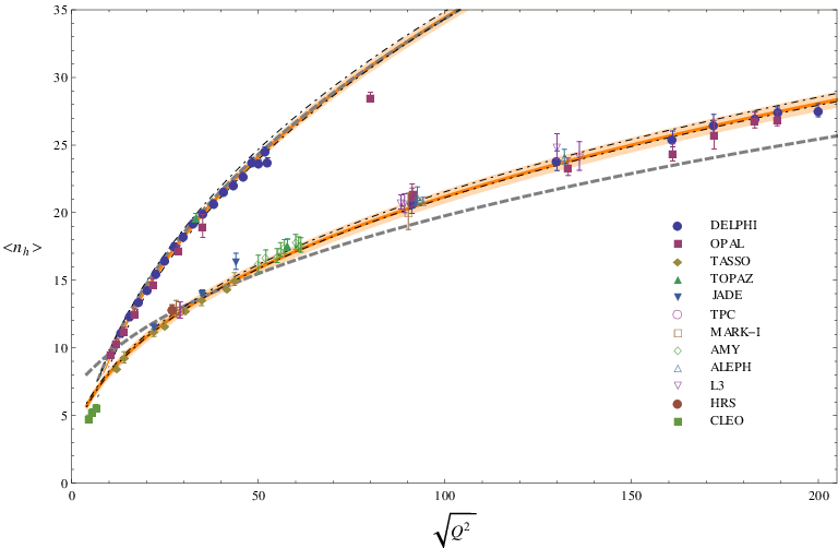
Now we show the results in [23] obtained from a global fit to the available experimental data of our formulas in Eq. (89) in the LO+NNLL\mathrm{LO}+\mathrm{NNLL}, N3​LOapprox+NNLL\mathrm{N}^{3}\mathrm{LO}_{\mathrm{approx}}+\mathrm{NNLL}, and N3​LOapprox+NLO+NNLL\mathrm{N}^{3}\mathrm{LO}_{\mathrm{approx}}+\mathrm{NLO}+\mathrm{NNLL} approximations, so as to extract the nonperturbative constants Dg​(0,Q02)D_{g}(0,Q^{2}_{0}) and Ds​(0,Q02)D_{s}(0,Q^{2}_{0}). We have to make a choice for the scale Q0Q_{0}, which, in principle, is arbitrary. In [23], we adopted Q0=50Q_{0}=50 GeV.

LO+NNLL\mathrm{LO}+\mathrm{NNLL} N3​LOapprox+NNLL\mathrm{N}^{3}\mathrm{LO}_{\mathrm{approx}}+\mathrm{NNLL} N3​LOapprox+NLO+NNLL\mathrm{N}^{3}\mathrm{LO}_{\mathrm{approx}}+\mathrm{NLO}+\mathrm{NNLL}
⟨nh​(Q02)⟩g\langle n_{h}(Q_{0}^{2})\rangle_{g} 24.31±0.8524.31\pm 0.85 24.02±0.3624.02\pm 0.36 24.17±0.3624.17\pm 0.36
⟨nh​(Q02)⟩q\langle n_{h}(Q_{0}^{2})\rangle_{q} 15.49±0.9015.49\pm 0.90 15.83±0.3715.83\pm 0.37 15.89±0.3315.89\pm 0.33
χdof2\chi_{\mathrm{dof}}^{2} \colorred 18.09 \colorred 3.71 \colorred 2.92
Table 3: Fit results for ⟨nh​(Q02)⟩g\langle n_{h}(Q_{0}^{2})\rangle_{g} and ⟨nh​(Q02)⟩q\langle n_{h}(Q_{0}^{2})\rangle_{q} at Q0=50Q_{0}=50 GeV with 90% CL errors and minimum values of χdof2\chi_{\mathrm{dof}}^{2} achieved in the LO+NNLL\mathrm{LO}+\mathrm{NNLL}, N3​LOapprox+NNLL\mathrm{N}^{3}\mathrm{LO}_{\mathrm{approx}}+\mathrm{NNLL}, and N3​LOapprox+NLO+NNLL\mathrm{N}^{3}\mathrm{LO}_{\mathrm{approx}}+\mathrm{NLO}+\mathrm{NNLL} approximations.

The gluon and quark AJMs extracted from experimental data strongly depend on the choice of jet algorithm. We adopt the selection of experimental data from Ref. [68] performed in such a way that they correspond to compatible jet algorithms. Specifically, these include the gluon AJM measurements in Refs. [68]-[72] and quark ones in Refs. [69, 73], which include 27 and 51 experimental data points, respectively. The results for ⟨nh​(Q02)⟩g\langle n_{h}(Q_{0}^{2})\rangle_{g} and ⟨nh​(Q02)⟩q\langle n_{h}(Q_{0}^{2})\rangle_{q} at Q0=50Q_{0}=50 GeV together with the χdof2\chi_{\mathrm{dof}}^{2} values obtained in our LO+NNLL\mathrm{LO}+\mathrm{NNLL}, N3​LOapprox+NNLL\mathrm{N}^{3}\mathrm{LO}_{\mathrm{approx}}+\mathrm{NNLL}, and N3​LOapprox+NLO+NNLL\mathrm{N}^{3}\mathrm{LO}_{\mathrm{approx}}+\mathrm{NLO}+\mathrm{NNLL} fits are listed in Table 3. The errors correspond to 90% CL as explained above. All these fit results are in agreement with the experimental data. Looking at the χdof2\chi_{\mathrm{dof}}^{2} values, we observe that the qualities of the fits improve as we go to higher orders, as they should. The improvement is most dramatic in the step from LO+NNLL\mathrm{LO}+\mathrm{NNLL} to N3​LOapprox+NNLL\mathrm{N}^{3}\mathrm{LO}_{\mathrm{approx}}+\mathrm{NNLL}, where the errors on ⟨nh​(Q02)⟩g\langle n_{h}(Q_{0}^{2})\rangle_{g} and ⟨nh​(Q02)⟩q\langle n_{h}(Q_{0}^{2})\rangle_{q} are more than halved. The improvement in the step from N3​LOapprox+NNLL\mathrm{N}^{3}\mathrm{LO}_{\mathrm{approx}}+\mathrm{NNLL} to N3​LOapprox+NLO+NNLL\mathrm{N}^{3}\mathrm{LO}_{\mathrm{approx}}+\mathrm{NLO}+\mathrm{NNLL}, albeit less pronounced, indicates that the inclusion of the first correction to r−​(Q2)r_{-}(Q^{2}) as given in Eq. (86) is favored by the experimental data. We have verified that the values of χdof2\chi_{\mathrm{dof}}^{2} are insensitive to the choice of Q0Q_{0}, as they should. Furthermore, the central values converge in the sense that the shifts in the step from N3​LOapprox+NNLL\mathrm{N}^{3}\mathrm{LO}_{\mathrm{approx}}+\mathrm{NNLL} to N3​LOapprox+NLO+NNLL\mathrm{N}^{3}\mathrm{LO}_{\mathrm{approx}}+\mathrm{NLO}+\mathrm{NNLL} are considerably smaller than those in the step from LO+NNLL\mathrm{LO}+\mathrm{NNLL} to N3​LOapprox+NNLL\mathrm{N}^{3}\mathrm{LO}_{\mathrm{approx}}+\mathrm{NNLL} and that, at the same time, the central values after each step are contained within error bars before that step. In the fits presented so far, the strong-coupling constant was taken to be the central value of the world avarage, αs(5)​(mZ2)=0.1184\alpha_{s}^{(5)}(m_{Z}^{2})=0.1184 [74]. In the next Section, we shall include αs(5)​(mZ2)\alpha_{s}^{(5)}(m_{Z}^{2}) among the fit parameters.

Refer to caption
Figure 4: The average gluon (upper curves) and quark (lower curves) jet multiplicities evaluated from Eq. (5.10), respectively, in the LO+NNLL\mathrm{LO}+\mathrm{NNLL} (dashed/gray lines) and N3​LOapprox+NLO+NNLL\mathrm{N}^{3}\mathrm{LO}_{\mathrm{approx}}+\mathrm{NLO}+\mathrm{NNLL} (solid/orange lines) approximations using the corresponding fit results for ⟨nh​(Q02)⟩g\langle n_{h}(Q_{0}^{2})\rangle_{g} and ⟨nh​(Q02)⟩q\langle n_{h}(Q_{0}^{2})\rangle_{q} from Table 3 are compared with the experimental data included in the fits. The experimental and theoretical uncertainties in the N3​LOapprox+NLO+NNLL\mathrm{N}^{3}\mathrm{LO}_{\mathrm{approx}}+\mathrm{NLO}+\mathrm{NNLL} results are indicated by the shaded/orange bands and the bands enclosed between the dot-dashed curves, respectively.

In Fig. 4, we show as functions of QQ the gluon and quark AJMs evaluated from Eq. (89) at LO+NNLL\mathrm{LO}+\mathrm{NNLL} and N3​LOapprox+NLO+NNLL\mathrm{N}^{3}\mathrm{LO}_{\mathrm{approx}}+\mathrm{NLO}+\mathrm{NNLL} using the corresponding fit results for ⟨nh​(Q02)⟩g\langle n_{h}(Q_{0}^{2})\rangle_{g} and ⟨nh​(Q02)⟩q\langle n_{h}(Q_{0}^{2})\rangle_{q} at Q0=50Q_{0}=50 GeV from Table 3. For clarity, we refrain from including in Fig. 4 the N3​LOapprox+NNLL\mathrm{N}^{3}\mathrm{LO}_{\mathrm{approx}}+\mathrm{NNLL} results, which are very similar to the N3​LOapprox+NLO+NNLL\mathrm{N}^{3}\mathrm{LO}_{\mathrm{approx}}+\mathrm{NLO}+\mathrm{NNLL} ones already presented in Ref. [22]. In the N3​LOapprox+NLO+NNLL\mathrm{N}^{3}\mathrm{LO}_{\mathrm{approx}}+\mathrm{NLO}+\mathrm{NNLL} case, Fig. 4 also displays two error bands, namely the experimental one induced by the 90% CL errors on the respective fit parameters in Table 3 and the theoretical one, which is evaluated by varying the scale parameter between Q/2Q/2 and 2​Q2Q.

Refer to caption
Figure 5: The average gluon-to-quark jet multiplicity ratio evaluated from Eq. (5.12) in the LO+NNLL\mathrm{LO}+\mathrm{NNLL} (dashed/gray lines) and N3​LOapprox+NLO+NNLL\mathrm{N}^{3}\mathrm{LO}_{\mathrm{approx}}+\mathrm{NLO}+\mathrm{NNLL} (solid/orange lines) approximations using the corresponding fit results for ⟨nh​(Q02)⟩g\langle n_{h}(Q_{0}^{2})\rangle_{g} and ⟨nh​(Q02)⟩q\langle n_{h}(Q_{0}^{2})\rangle_{q} from Table 3 are compared with experimental data. The experimental and theoretical uncertainties in the N3​LOapprox+NLO+NNLL\mathrm{N}^{3}\mathrm{LO}_{\mathrm{approx}}+\mathrm{NLO}+\mathrm{NNLL} result are indicated by the shaded/orange bands and the bands enclosed between the dot-dashed curves, respectively. The prediction given by Eq. (5.8) [25] is indicated by the continuous/gray line.

While our fits rely on individual measurements of the gluon and quark AJMs, the experimental literature also reports determinations of their ratio; see Refs. [27, 68, 70, 72, 75], which essentially cover all the available measurements. In order to find out how well our fits describe the latter and thus to test the global consistency of the individual measurements, we compare in Fig. 5 the experimental data on the gluon-to-quark AJM ratio with our evaluations of Eq. (91) in the LO+NNLL\mathrm{LO}+\mathrm{NNLL} and N3​LOapprox+NLO+NNLL\mathrm{N}^{3}\mathrm{LO}_{\mathrm{approx}}+\mathrm{NLO}+\mathrm{NNLL} approximations using the corresponding fit results from Table 3. As in Fig. 4, we present in Fig. 5 also the experimental and theoretical uncertainties in the N3​LOapprox+NLO+NNLL\mathrm{N}^{3}\mathrm{LO}_{\mathrm{approx}}+\mathrm{NLO}+\mathrm{NNLL} result. For comparison, we include in Fig. 5 also the prediction of Ref. [25] given by Eq. (87).

Looking at Fig. 5, we observe that the experimental data are very well described by the N3​LOapprox+NLO+NNLL\mathrm{N}^{3}\mathrm{LO}_{\mathrm{approx}}+\mathrm{NLO}+\mathrm{NNLL} result for QQ values above 10 GeV, while they somewhat overshoot it below. This discrepancy is likely to be due to the fact that, following Ref. [68], we excluded the older data from Ref. [27] from our fits because they are inconsistent with the experimental data sample compiled in Ref. [68].

The Monte Carlo analysis of Ref. [26] suggests that the average gluon and quark jet multiplicities should coincide at about Q=4Q=4 GeV. As is evident from Fig. 5, this agrees with our N3​LOapprox+NLO+NNLL\mathrm{N}^{3}\mathrm{LO}_{\mathrm{approx}}+\mathrm{NLO}+\mathrm{NNLL} result reasonably well given the considerable uncertainties in the small-Q2Q^{2} range discussed above.

Refer to caption
Figure 6: High-QQ extension of Fig. 5.

As is obvious from Fig. 5, the approximation of r⁡(Q2)r(Q^{2}) by r+​(Q2)r_{+}(Q^{2}) given in Eq. (87) [25] leads to a poor approximation of the experimental data, which reach up to QQ values of about 50 GeV. It is, therefore, interesting to study the high-Q2Q^{2} asymptotic behavior of the average gluon-to-quark jet ratio. This is done in Fig. 6, where the N3​LOapprox+NLO+NNLL\mathrm{N}^{3}\mathrm{LO}_{\mathrm{approx}}+\mathrm{NLO}+\mathrm{NNLL} result including its experimental and theoretical uncertainties is compared with the approximation by Eq. (87) way up to Q=100Q=100 TeV. We observe from Fig. 6 that the approximation approaches the N3​LOapprox+NLO+NNLL\mathrm{N}^{3}\mathrm{LO}_{\mathrm{approx}}+\mathrm{NLO}+\mathrm{NNLL} result rather slowly. Both predictions agree within theoretical errors at Q=100Q=100 TeV, which is one order of magnitude beyond LHC energies, where they are still about 10% below the asymptotic value CA/CF=2.25C_{A}/C_{F}=2.25.

6.2.1 Determination of strong-coupling constant from average multiplicity

N3​LOapprox+NNLL\mathrm{N}^{3}\mathrm{LO}_{\mathrm{approx}}+\mathrm{NNLL} N3​LOapprox+NLO+NNLL\mathrm{N}^{3}\mathrm{LO}_{\mathrm{approx}}+\mathrm{NLO}+\mathrm{NNLL}
⟨nh​(Q02)⟩g\langle n_{h}(Q_{0}^{2})\rangle_{g} 24.18±0.3224.18\pm 0.32 24.22±0.3324.22\pm 0.33
⟨nh​(Q02)⟩q\langle n_{h}(Q_{0}^{2})\rangle_{q} 15.86±0.3715.86\pm 0.37 15.88±0.3515.88\pm 0.35
αs(5)​(mZ2)\alpha_{s}^{(5)}(m_{Z}^{2}) 0.1242±0.00460.1242\pm 0.0046 0.1199±0.00440.1199\pm 0.0044
χdof2\chi_{\mathrm{dof}}^{2} \colorred 2.84 \colorred 2.85
Table 4: Fit results for ⟨nh​(Q02)⟩g\langle n_{h}(Q_{0}^{2})\rangle_{g} and ⟨nh​(Q02)⟩q\langle n_{h}(Q_{0}^{2})\rangle_{q} at Q0=50Q_{0}=50 GeV and for αs(5)​(mZ2)\alpha_{s}^{(5)}(m_{Z}^{2}) with 90% CL errors and minimum values of χdof2\chi_{\mathrm{dof}}^{2} achieved in the N3​LOapprox+NNLL\mathrm{N}^{3}\mathrm{LO}_{\mathrm{approx}}+\mathrm{NNLL} and N3​LOapprox+NLO+NNLL\mathrm{N}^{3}\mathrm{LO}_{\mathrm{approx}}+\mathrm{NLO}+\mathrm{NNLL} approximations.

In the previous Section, we took αs(5)​(mZ2)\alpha_{s}^{(5)}(m_{Z}^{2}) to be a fixed input parameter for our fits. Motivated by the excellent goodness of our N3​LOapprox+NNLL\mathrm{N}^{3}\mathrm{LO}_{\mathrm{approx}}+\mathrm{NNLL} and N3​LOapprox+NLO+NNLL\mathrm{N}^{3}\mathrm{LO}_{\mathrm{approx}}+\mathrm{NLO}+\mathrm{NNLL} fits, we now include it among the fit parameters, the more so as the fits should be sufficiently sensitive to it in view of the wide Q2Q^{2} range populated by the experimental data fitted to. We fit to the same experimental data as before and again put Q0=50Q_{0}=50 GeV. The fit results are summarized in Table 4. We observe from Table 4 that the results of the N3​LOapprox+NNLL\mathrm{N}^{3}\mathrm{LO}_{\mathrm{approx}}+\mathrm{NNLL} [51] and N3​LOapprox+NLO+NNLL\mathrm{N}^{3}\mathrm{LO}_{\mathrm{approx}}+\mathrm{NLO}+\mathrm{NNLL} fits for ⟨nh​(Q02)⟩g\langle n_{h}(Q_{0}^{2})\rangle_{g} and ⟨nh​(Q02)⟩q\langle n_{h}(Q_{0}^{2})\rangle_{q} are mutually consistent. They are also consistent with the respective fit results in Table 3. As expected, the values of χdof2\chi_{\mathrm{dof}}^{2} are reduced by relasing αs(5)​(mZ2)\alpha_{s}^{(5)}(m_{Z}^{2}) in the fits, from 3.71 to 2.84 in the N3​LOapprox+NNLL\mathrm{N}^{3}\mathrm{LO}_{\mathrm{approx}}+\mathrm{NNLL} approximation and from 2.95 to 2.85 in the N3​LOapprox+NLO+NNLL\mathrm{N}^{3}\mathrm{LO}_{\mathrm{approx}}+\mathrm{NLO}+\mathrm{NNLL} one. The three-parameter fits strongly confine αs(5)​(mZ2)\alpha_{s}^{(5)}(m_{Z}^{2}), within an error of 3.7% at 90% CL in both approximations. The inclusion of the r−​(Q2)r_{-}(Q^{2}) term has the beneficial effect of shifting αs(5)​(mZ2)\alpha_{s}^{(5)}(m_{Z}^{2}) closer to the world average, 0.1184±0.00070.1184\pm 0.0007 [74]. In fact, our N3​LOapprox+NLO+NNLL\mathrm{N}^{3}\mathrm{LO}_{\mathrm{approx}}+\mathrm{NLO}+\mathrm{NNLL} value, 0.1199±0.00440.1199\pm 0.0044 at 90% CL, which corresponds to 0.1199±0.00260.1199\pm 0.0026 at 68% CL, is in excellent agreement with the former. Note that similar αs(5)​(mZ2)\alpha_{s}^{(5)}(m_{Z}^{2}) valu has been otained recently [76] in an extension of the MLLA approach.

7 Conclusions

We have shown the Q2Q^{2}-dependences of the SF F2F_{2} at small-xx values and of AJMs in the framework of perturbative QCD. We would like to stress that a good agreement wit the experimental data for the variables cannot be obtained without a proper consideration of the cotributions of both the “++” and “−-” components.

The “++” components contain all large logarithms ln⁡(1/x)\ln(1/x) as far as DIS SF F2F_{2} and also for the average jet multiplicities. The large logarithms are resummed using famous BFKL approach [8] in the PDF case and another famous MLLA approach [50] in the FF case. 1414 14 Note, however, that in the case of DIS SF F2F_{2} we use obly the first two orders of the perturbation theory and our “++” component resum by DGLAP equation [6]. The resummation leads to the Bessel-like form of the “++” component. Including all orders of the perturbation theory should lead to a power-like form as it was predicted in the framework of BFKL approach [8] (see discussion in [54]). Nevertheless, the contributions of the “−-” components are very important to have a good agreement with experimental data: they come with the additional free parameters. Moreover, the “−-” components have other shapes to compare with the “++” ones. For example, in the AJM case the “−-” component is responsable for the difference in the Q2Q^{2}-dependences of quark and gluon multiplicities. Indeed, the “−-” component gives essential contribution to the quark AJM but not to the gluon one.

In the case of DIS SF F2F_{2}, our results are in very good agreement with precise HERA data at Q2≥2÷3Q^{2}\geq 2\div 3 GeV2, where perturbative theory can be applicable. The application of the “frozen” and analytic coupling constants αfr​(Q2)\alpha_{\rm fr}(Q^{2}) and αan​(Q2)\alpha_{\rm an}(Q^{2}) improves the agreement with the recent HERA data [3] for small Q2Q^{2} values, Q2≥0.5Q^{2}\geq 0.5 GeV2.

Prior to our analysis in Ref. [22, 23], experimental data on the gluon and quark AJMs could not be simultaneously described in a satisfactory way mainly because the theoretical formalism failed to account for the difference in hadronic contents between gluon and quark jets, although the convergence of perturbation theory seemed to be well under control [25]. This problem was solved by including the “−-” components governed by T^−res​(0,Q2,Q02)\hat{T}_{-}^{\mathrm{res}}(0,Q^{2},Q_{0}^{2}) in Eqs. (89) and (91). This was done for the first time in Ref. [22]. The quark-singlet “−-” component comes with an arbitrary normalization and has a slow Q2Q^{2} dependence. Consequently, its numerical contribution may be approximately mimicked by a constant introduced to the average quark jet multiplicity as in Ref. [27].

Motivated by the goodness of our fits in [22, 23] with fixed value of αs(5)​(mZ2)\alpha_{s}^{(5)}(m_{Z}^{2}), we then included αs(5)​(mZ2)\alpha_{s}^{(5)}(m_{Z}^{2}) among the fit parameters, which yielded a further reduction of χdof2\chi_{\mathrm{dof}}^{2}. The fit results are listed in Table 4.

Acknowledgments
This work was supported by RFBR grant 13-02-01005-a. Author thanks the Organizing Committee of XXII International Baldin Seminar on High Energy Physics Problems for invitation.

References

  • [1] C. Adloff et al. [H1 Collaboration], Nucl. Phys. B 497 (1997) 3; Eur. Phys. J. C 21 (2001) 33.
  • [2] S. Chekanov et al. [ZEUS Collaboration], Eur. Phys. J. C 21 (2001) 443.
  • [3] F. D. Aaron et al. [H1 and ZEUS Collaboration], JHEP 1001 (2010) 109.
  • [4] B. Surrow [H1 and ZEUS Collaboration], Phenomenological studies of inclusive e p scattering at low momentum transfer Q**2, hep-ph/0201025; C. Adloff et al. [H1 Collaboration], Phys. Lett. B 520 (2001) 183; T. Lastovicka [H1 Collaboration], Acta Phys. Polon. B 33 (2002) 2835; J. Gayler [H1 Collaboration], Acta Phys. Polon. B 33 (2002) 2841.
  • [5] F. D. Aaron et al. [H1 Collaboration], Phys. Lett. B 686 (2010) 91; Eur. Phys. J. C 65 (2010) 89; H. Abramowicz et al. [ZEUS collaboration], Eur. Phys. J. C 69 (2010) 347; S. Chekanov et al. [ZEUS Collaboration], Eur. Phys. J. C 65 (2010) 65; K. Lipka [H1 Collaboration and ZEUS Collaboration], Nucl. Phys. Proc. Suppl. 191 (2009) 163; H. Abramowicz et al. [H1 and ZEUS Collaborations], Eur. Phys. J. C 73 (2013) 2, 2311.
  • [6] V. N. Gribov and L. N. Lipatov, Sov. J. Nucl. Phys. 15 (1972) 438, 675; L. N. Lipatov, Sov. J. Nucl. Phys. 20 (1975) 94; G. Altarelli and G. Parisi, Nucl. Phys. B 126 (1977) 298; Yu. L. Dokshitzer, Sov. Phys. JETP 46 (1977) 641.
  • [7] A. M. Cooper-Sarkar, R. C. E. Devenish, and A. De Roeck, Int. J. Mod. Phys. A 13 (1998) 3385; A. V. Kotikov, Phys. Part. Nucl. 38 (2007) 1. [Erratum-ibid. 38 (2007) 828]; S. Alekhin et al., “HERAFitter, Open Source QCD Fit Project,” arXiv:1410.4412 [hep-ph]; J. Butterworth et al., “Les Houches 2013: Physics at TeV Colliders: Standard Model Working Group Report,” arXiv:1405.1067 [hep-ph]; P. Belov et al. [HERAFitter developers’ team Collaboration], Eur. Phys. J. C 74 (2014) 10, 3039.
  • [8] L. N. Lipatov, Sov. J. Nucl. Phys. 23 (1976) 338; E. A. Kuraev, L. N. Lipatov, and V. S. Fadin, Phys. Lett. B 60 (1975) 50; Sov. Phys. JETP 44 (1976) 443; 45 (1977) 199; Ya. Ya. Balitzki and L. N. Lipatov, Sov. J. Nucl. Phys. 28 (1978) 822; L. N. Lipatov, Sov. Phys. JETP 63 (1986) 904.
  • [9] J. Gao, M. Guzzi, J. Huston, H. L. Lai, Z. Li, P. Nadolsky, J. Pumplin and D. Stump et al., Phys. Rev. D 89 (2014) 3, 033009; A. D. Martin, W. J. Stirling, R. S. Thorne and G. Watt, Eur. Phys. J. C 64 (2009) 653; A. D. Martin, A. J. T. M. Mathijssen, W. J. Stirling, R. S. Thorne, B. J. A. Watt and G. Watt, Eur. Phys. J. C 73 (2013) 2, 2318; S. Alekhin, J. Blumlein and S. Moch, Phys. Rev. D 86 (2012) 054009; Phys. Rev. D 89 (2014) 5, 054028; R. D. Ball, V. Bertone, L. Del Debbio, S. Forte, A. Guffanti, J. I. Latorre, S. Lionetti and J. Rojo et al., Phys. Lett. B 707 (2012) 66; R. D. Ball, V. Bertone, S. Carrazza, C. S. Deans, L. Del Debbio, S. Forte, A. Guffanti and N. P. Hartland et al., Nucl. Phys. B 867 (2013) 244.
  • [10] P. Jimenez-Delgado and E. Reya, Phys. Rev. D 80 (2009) 114011; Phys. Rev. D 79 (2009) 074023; Phys. Rev. D 89 (2014) 7, 074049.
  • [11] A. V. Kotikov, G. Parente, and J. Sanchez Guillen, Z. Phys. C 58 (1993) 465; G. Parente, A. V. Kotikov, and V. G. Krivokhizhin, Phys. Lett. B 333 (1994) 190; A. L. Kataev, A. V. Kotikov, G. Parente, and A. V. Sidorov, Phys. Lett. B 388 (1996) 179; Phys. Lett. B 417 (1998) 374; A. L. Kataev, G. Parente, and A. V. Sidorov, Nucl. Phys. B 573 (2000) 405; A. V. Kotikov and V. G. Krivokhijine, Phys. At. Nucl. 68 (2005) 1873; B. G. Shaikhatdenov, A. V. Kotikov, V. G. Krivokhizhin and G. Parente, Phys. Rev. D 81 (2010) 034008; A. V. Kotikov, V. G. Krivokhizhin and B. G. Shaikhatdenov, arXiv:1411.1236 [hep-ph].
  • [12] A. V. Kotikov, V. G. Krivokhizhin and B. G. Shaikhatdenov, Phys. Atom. Nucl. 75 (2012) 507; A. V. Sidorov and O. P. Solovtsova, Mod. Phys. Lett. A 29 (2014) 36, 1450194;
  • [13] R. D. Ball and S. Forte, Phys. Lett. B 336 (1994) 77.
  • [14] L. Mankiewicz, A. Saalfeld, and T. Weigl, Phys. Lett. B 393 (1997) 175.
  • [15] A. V. Kotikov and G. Parente, Nucl. Phys. B 549 (1999) 242; Nucl. Phys. (Proc. Suppl.) A 99 (2001) 196. [hep-ph/0010352].
  • [16] A. Yu. Illarionov, A. V. Kotikov, and G. Parente, Phys. Part. Nucl. 39 (2008) 307; Nucl. Phys. (Proc. Suppl.) 146 (2005) 234.
  • [17] A. De Rújula, S. L. Glashow, H. D. Politzer, S.B. Treiman, F. Wilczek, and A. Zee, Phys. Rev. D 10, 1649 (1974) 1649.
  • [18] A. H. Mueller, Phys. Lett. B 104 (1981) 161.
  • [19] A. Vogt, JHEP 1110 (2011) 025.
  • [20] S. Albino, P. Bolzoni, B. A. Kniehl and A. V. Kotikov, Nucl. Phys. B 855 (2012) 801.
  • [21] C.-H. Kom, A. Vogt and K. Yeats, JHEP 1210 (2012) 033.
  • [22] P. Bolzoni, B. A. Kniehl and A. V. Kotikov, Phys. Rev. Lett. 109 (2012) 242002.
  • [23] P. Bolzoni, B. A. Kniehl and A. V. Kotikov, Nucl. Phys. B 875 (2013) 18.
  • [24] S. Albino, P. Bolzoni, B. A. Kniehl and A. Kotikov, arXiv:1107.1142 [hep-ph]; Nucl. Phys. B 851 (2011) 86.
  • [25] A. Capella, I. M. Dremin, J. W. Gary, V. A. Nechitailo and J. Tran Thanh Van, Phys. Rev. D 61 (2000) 074009.
  • [26] P. Eden and G. Gustafson, JHEP 9809 (1998) 015 [hep-ph/9805228].
  • [27] P. Abreu et al. [DELPHI Collaboration], Phys. Lett. B 449 (1999) 383 [hep-ex/9903073].
  • [28] P. Bolzoni, arXiv:1206.3039 [hep-ph], DOI: 10.3204/DESY-PROC-2012-02/96.
  • [29] J.A.M. Vermaseren, A. Vogt, S. Moch, Nucl.Phys.B724 (2005) 3.
  • [30] A. J. Buras, Rev. Mod. Phys. 52 (1980) 199.
  • [31] D. I. Kazakov and A. V. Kotikov, Nucl. Phys. B 307 (1988) 721 [Erratum-ibid. B 345 (1990) 299]; Phys. Lett. B 291 (1992) 171; A. V. Kotikov, Phys. Atom. Nucl. 57 (1994) 133 [Yad. Fiz. 57 (1994) 142]; A. V. Kotikov and V. N. Velizhanin, Analytic continuation of the Mellin moments of deep inelastic structure functions, hep-ph/0501274.
  • [32] F.J. Yndurain, Quantum Chromodynamics (An Introduaction to the Theory of Quarks and Gluons).-Berlin, Springer-Verlag (1983).
  • [33] A. V. Kotikov, Phys. Atom. Nucl. 56 (1993) 1276.
  • [34] J.A.M. Vermaseren, A. Vogt, S. Moch, Nucl.Phys.B688 (2004) 101.
  • [35] R. K. Ellis, W. J. Stirling and B. R. Webber, Camb. Monogr. Part. Phys. Nucl. Phys. Cosmol. 8 (1996) 1.
  • [36] M. Glück, E. Reya and A. Vogt, Phys. Rev. D 48 (1993) 116 [Erratum-ibid. D 51 (1995) 1427].
  • [37] S. Moch and A. Vogt, Phys. Lett. B 659 (2008) 290.
  • [38] A. A. Almasy, S. Moch and A. Vogt, Nucl. Phys. B 854 (2012) 133.
  • [39] A. V. Kotikov and L. N. Lipatov, Nucl. Phys. B 661 (2003) 19; in: Proc. of the XXXV Winter School, Repino, S’Peterburg, 2001 (hep-ph/0112346).
  • [40] B. I. Ermolaev and V. S. Fadin, Pis’ma Zh. Eksp. Teor. Fiz. 33 (1981) 285 [JETP Lett. 33 (1981) 269]; Yu. L. Dokshitzer, V. S. Fadin and V. A. Khoze, Z. Phys. C 15 (1982) 325; Phys. Lett. B 115 (1982) 242; Z. Phys. C 18 (1983) 37.
  • [41] V. S. Fadin and L. N. Lipatov, Phys. Lett. B 429 (1998) 127; G. Camici and M. Ciafaloni, Phys. Lett. B430 (1998) 349.
  • [42] A. V. Kotikov and L. N. Lipatov, Nucl. Phys. B 582 (2000) 19.
  • [43] M. Ciafaloni, D. Colferai, G. P. Salam and A. M. Stasto, JHEP 0708 (2007) 046; G. Altarelli, R. D. Ball and S. Forte, Nucl. Phys. B 799 (2008) 199.
  • [44] A. H. Mueller, Nucl. Phys. B 241 (1984) 141.
  • [45] M. Schmelling, Phys. Scripta 51 (1995) 683.
  • [46] I. M. Dremin and J. W. Gary, Phys. Rept. 349 (2001) 301.
  • [47] A. Yu. Illarionov, A. V. Kotikov and G. Parente, Phys. Part. Nucl. 39 (2008) 307.
  • [48] G. Cvetic, A. Yu. Illarionov, B. A. Kniehl and A. V. Kotikov, Phys. Lett. B 679 (2009) 350; A. V. Kotikov and B. G. Shaikhatdenov, Phys. Part. Nucl. 44 (2013) 543; AIP Conf. Proc. 1606 (2014) 159 [arXiv:1402.3703 [hep-ph]].
  • [49] I. M. Dremin and J. W. Gary, Phys. Lett. B 459 (1999) 341.
  • [50] Yu. L. Dokshitzer, V. A. Khoze, A. H. Mueller and S. I. Troyan, Basics of perturbative QCD, Editions Frontières, edited by J. Tran Thanh Van, (Fong and Sons Printers Pte. Ltd., Singapore, 1991).
  • [51] P. Bolzoni, arXiv:1211.5550 [hep-ph].
  • [52] A. V. Kotikov and G. Parente, J. Exp. Theor. Phys. 97 (2003) 859.
  • [53] A. Y. .Illarionov and A. V. Kotikov, Phys. Atom. Nucl. 75 (2012) 1234; A. Y. Illarionov, B. A. Kniehl and A. V. Kotikov, Phys. Lett. B 663 (2008) 66.
  • [54] A. V. Kotikov, PoS Baldin -ISHEPP-XXI (2012) 033 [arXiv:1212.3733 [hep-ph]].
  • [55] A. Y. .Illarionov, B. A. Kniehl and A. V. Kotikov, Phys. Rev. Lett. 106 (2011) 231802.
  • [56] G. Grunberg, Phys. Rev. D 29 (1984) 2315; Phys. Lett. B 95 (1980) 70.
  • [57] Yu. L. Dokshitzer and D. V. Shirkov, Z. Phys. C 67 (1995) 449; A. V. Kotikov, JETP Lett. 59 (1994) 1; Phys. Lett. B 338 (1994) 349; W. K. Wong, Phys. Rev. D 54 (1996) 1094.
  • [58] S. J. Brodsky, V. S. Fadin, V. T. Kim, L.N. Lipatov, G.B. Pivovarov, JETP. Lett. 70 (1999) 155; M. Ciafaloni, D. Colferai, and G. P. Salam, Phys. Rev. D 60 (1999) 114036 ; JHEP 07 (2000) 054; R. S. Thorne, Phys. Lett. B 474 (2000) 372; Phys. Rev. D 60 (1999) 054031; 64 (2001) 074005; G. Altarelli, R. D. Ball, and S. Forte, Nucl. Phys. B 621 (2002) 359.
  • [59] Bo Andersson et al., Eur. Phys. J. C 25 (2002) 77.
  • [60] A. V. Kotikov and B. G. Shaikhatdenov, arXiv:1402.4349 [hep-ph], Phys. Atom. Nucl. (2015) in press.
  • [61] G. Curci, M. Greco, and Y. Srivastava, Phys. Rev. Lett. 43 (1979) 834; Nucl. Phys. B 159 (1979) 451; M. Greco, G. Penso, and Y. Srivastava, Phys. Rev. D 21 (1980) 2520; PLUTO Collab. (C. Berger et al.), Phys. Lett. B 100 (1981) 351; N. N. Nikolaev and B. M. Zakharov, Z. Phys. C 49 (1991) 607; 53 (1992) 331; B. Badelek, J. Kwiecinski, and A. Stasto, Z. Phys. C 74 (1997) 297.
  • [62] D. V. Shirkov and I. L. Solovtsov, Phys. Rev. Lett 79 (1997) 1209; Theor. Math. Phys. 120 (1999) 1220.
  • [63] A. V. Nesterenko, Phys. Rev. D 64 (2001) 116009; Int. J. Mod. Phys. A18 (2003) 5475; A. V. Nesterenko and J. Papavassiliou, Phys. Rev. D 71 (2005) 016009; J. Phys. G 32 (2006) 1025; G. Cvetic, C. Valenzuela, and I. Schmidt, Nucl. Phys. Proc. Suppl. 164 (2007) 308; G. Cvetic and C. Valenzuela, J. Phys. G 32 (2006) L27; Phys. Rev. D 74 (2006) 114030; Phys. Rev. D 77 (2008) 074021; A. P. Bakulev, S. V. Mikhailov, and N. G. Stefanis, Phys. Rev. D 72 (2005) 074014; Phys. Rev. D 75 (2007) 056005; G. Cvetic and A. V. Kotikov, J. Phys. G 39 (2012) 065005.
  • [64] R. S. Pasechnik, D. V. Shirkov, and O. V. Teryaev, Phys. Rev. D 78 (2008) 071902; R. S. Pasechnik, D. V. Shirkov, O. V. Teryaev, O. P. Solovtsova and V. L. Khandramai, Phys. Rev. D 81 (2010) 016010; V. L. Khandramai, R. S. Pasechnik, D. V. Shirkov, O. P. Solovtsova and O. V. Teryaev, Phys. Lett. B 706 (2012) 340; A. V. Kotikov and B. G. Shaikhatdenov, Phys. Part. Nucl. 45 (2014) 26 [arXiv:1212.6834 [hep-ph]].
  • [65] G. Cvetic and C. Valenzuela, Braz. J. Phys. 38 (2008) 371; A. P. Bakulev, S. V. Mikhailov, Resummation in (F)APT arXiv:0803.3013 [hep-ph]; N. G. Stefanis, Phys. Part. Nucl. 44 (2013) 494.
  • [66] A. V. Kotikov, A. V. Lipatov, and N. P. Zotov, J. Exp. Theor. Phys. 101 (2005) 811.
  • [67] H. Kowalski, L. N. Lipatov and D. A. Ross, Phys. Part. Nucl. 44 (2013) 547.
  • [68] J. Abdallah et al. [DELPHI Collaboration], Eur. Phys. J. C 44 (2005) 311.
  • [69] K. Nakabayashi et al. [TOPAZ Collaboration], Phys. Lett. B 413 (1997) 447.
  • [70] G. Abbiendi et al. [OPAL Collaboration], Eur. Phys. J. C 11 (1999) 217.
  • [71] G. Abbiendi et al. [OPAL Collaboration], Eur. Phys. J. C 37 (2004) 25.
  • [72] M. Siebel, Ph.D. Thesis No. WUB-DIS 2003-11, Bergische Universität Wuppertal, November 2003.
  • [73] S. Kluth et al. [JADE Collaboration], hep-ex/0305023; M. Althoff et al. [TASSO Collaboration], Z. Phys. C 22 (1984) 307; W. Braunschweig et al. [TASSO Collaboration], Z. Phys. C 45 (1989) 193; H. Aihara et al. [TPC/Two Gamma Collaboration], Phys. Lett. B 184 (1987) 299; P. C. Rowson et al., Phys. Rev. Lett. 54 (1985) 2580; M. Derrick et al., Phys. Rev. D 34 (1986) 3304; H. W. Zheng et al. [AMY Collaboration], Phys. Rev. D 42 (1990) 737; G. S. Abrams et al., Phys. Rev. Lett. 64 (1990) 1334; D. Decamp et al. [ALEPH Collaboration], Phys. Lett. B 234 (1990) 209; Phys. Lett. B 273 (1991) 181; D. Buskulic et al. [ALEPH Collaboration], Z. Phys. C 69 (1995) 15; Z. Phys. C 73 (1997) 409; R. Barate et al. [ALEPH Collaboration], Phys. Rept. 294 (1998) 1; P. Abreu et al. [DELPHI Collaboration], Z. Phys. C 50 (1991) 185; Z. Phys. C 52 (1991) 271; Eur. Phys. J. C 5 (1998) 585; Phys. Lett. B 372 (1996) 172; Phys. Lett. B 416 (1998) 233; Eur. Phys. J. C 18 (2000) 203 [Erratum-ibid. C 25 (2002) 493]; B. Adeva et al. [L3 Collaboration], Phys. Lett. B 259 (1991) 199; Z. Phys. C 55 (1992) 39; M. Z. Akrawy et al. [OPAL Collaboration], Z. Phys. C 47 (1990) 505; P. D. Acton et al. [OPAL Collaboration], Phys. Lett. B 291 (1992) 503; Z. Phys. C 53 (1992) 539; K. Ackerstaff et al. [OPAL Collaboration], Eur. Phys. J. C 7 (1999) 369; Z. Phys. C 75 (1997) 193; M. Acciarri et al. [L3 Collaboration], Phys. Lett. B 371 (1996) 137; G. Alexander et al. [OPAL Collaboration], Z. Phys. C 72 (1996) 191; G. Abbiendi et al. [OPAL Collaboration], Eur. Phys. J. C 16 (2000) 185.
  • [74] J. Beringer et al. [Particle Data Group Collaboration], Phys. Rev. D 86 (2012) 010001.
  • [75] M. S. Alam et al. [CLEO Collaboration], Phys. Rev. D 56 (1997) 17; Phys. Rev. D 46 (1992) 4822; H. Albrecht et al. [ARGUS Collaboration], Z. Phys. C 54 (1992) 13; D. Acosta et al. [CDF Collaboration], Phys. Rev. Lett. 94 (2005) 171802; M. Derrick et al., Phys. Lett. B 165 (1985) 449; W. Braunschweig et al. [TASSO Collaboration], Z. Phys. C 45 (1989) 1; G. Alexander et al. [OPAL Collaboration], Phys. Lett. B 265, 462 (1991); Phys. Lett. B 388 (1996) 659; P. D. Acton et al. [OPAL Collaboration], Z. Phys. C 58, 387 (1993); R. Akers et al. [OPAL Collaboration], Z. Phys. C 68, 179 (1995); O. Biebel [OPAL Collaboration], in DPF‘96: The Minneapolis Meeting, edited by K. Heller, J. K. Nelson, and D. Reeder (World Scientific Publishing Co. Pte. Ltd., Singapore, 1998), Volume 1, p. 354–356; D. Buskulic et al. [ALEPH Collaboration], Phys. Lett. B 384 (1996) 353; P. Abreu et al. [DELPHI Collaboration], Z. Phys. C 70 (1996) 179; K. Ackerstaff et al. [OPAL Collaboration], Eur. Phys. J. C 1 (1998) 479; G. Abbiendi et al. [OPAL Collaboration], Phys. Rev. D 69 (2004) 032002.
  • [76] R. Perez-Ramos and D. d’Enterria, JHEP 1408 (2014) 068; arXiv:1410.4818 [hep-ph]; arXiv:1412.2102 [hep-ph].

8 Appendix A

For diagonalization of quark and gluon interaction it is neseccary to introduce the corresponding matrix UU, which diagonalize exactly the LO AD

U^−1​(γq​q(0)​(n)γg​q(0)​(n)γq​g(0)​(n)γg​g(0)​(n))​U^=(γ−(0)​(n)00γ+(0)​(n))(U^−1​U^=1),\displaystyle\hat{U}^{-1}\left(\begin{array}[]{cc}\gamma^{(0)}_{qq}(n)&\gamma^{(0)}_{gq}(n)\\ \gamma^{(0)}_{qg}(n)&\gamma^{(0)}_{gg}(n)\end{array}\right)\hat{U}~=~\left(\begin{array}[]{cc}\gamma^{(0)}_{-}(n)&0\\ 0&\gamma^{(0)}_{+}(n)\end{array}\right)~~~~~\left(\hat{U}^{-1}\hat{U}=1\right),

where

U^=(αnαn−1βnβn),U^−1=(11−αnβn−11​αnβn)\displaystyle\hat{U}~=~\left(\begin{array}[]{cc}\alpha_{n}&\alpha_{n}-1\\ \beta_{n}&\beta_{n}\end{array}\right),~~\hat{U}^{-1}~=~\left(\begin{array}[]{cc}1&\frac{1-\alpha_{n}}{\beta_{n}}\\ -1&\frac{1\alpha_{n}}{\beta_{n}}\end{array}\right)

and αn\alpha_{n} and βn\beta_{n} have been defined in the main text, in Eq. (19).

At higher orders the anomalous dimensions are transformed as follows

U^−1​(γq​q(i)​(n)γg​q(i)​(n)γq​g(i)​(n)γg​g(i)​(n))​U^=(γ−⁣−(n)​(j)γ−⁣+(i)​(n)γ+⁣−(i)​(n)γ+⁣+(i)​(n)),\displaystyle\hat{U}^{-1}\left(\begin{array}[]{cc}\gamma^{(i)}_{qq}(n)&\gamma^{(i)}_{gq}(n)\\ \gamma^{(i)}_{qg}(n)&\gamma^{(i)}_{gg}(n)\end{array}\right)\hat{U}~=~\left(\begin{array}[]{cc}\gamma^{(n)}_{--}(j)&\gamma^{(i)}_{-+}(n)\\ \gamma^{(i)}_{+-}(n)&\gamma^{(i)}_{++}(n)\end{array}\right)~,

where exact representations for γ±⁣±(i)​(n)\gamma^{(i)}_{\pm\pm}(n) and γ±⁣∓(i)​(n)\gamma^{(i)}_{\pm\mp}(n) were given in the main text, in Eq. (23).

8.1 Diagonalization of the renormalization group exponent

Consider the renormalization group exponent (hereafter in the Appendix A a¯s=as​(Q2)\overline{a}_{s}=a_{s}(Q^{2}) and as=as​(Q02)a_{s}=a_{s}(Q^{2}_{0}))

W^​(as,a¯s)≡Tas​exp⁡[∫a¯sasd​a′a′​γ^​(a′)2​β​(a′)],\hat{W}(a_{s},\overline{a}_{s})\equiv T_{a_{s}}\,\exp\,\left[\int^{a_{s}}_{\overline{a}_{s}}\,\frac{da^{\prime}}{a^{\prime}}\frac{\hat{\gamma}(a^{\prime})}{2\beta(a^{\prime})}\right], (A16)

in the following form

W^​(as,a¯s)=V^​(as)​exp⁡[γ^(0)​(n)2​β0​ln⁡a¯sas]​V^−1​(a¯s)≡V^​(as)​W^(0)​(as,a¯s)​V^−1​(a¯s),\hat{W}(a_{s},\overline{a}_{s})=\hat{V}(a_{s})\,\exp\,\left[\frac{\hat{\gamma}^{(0)}(n)}{2\beta_{0}}\ln\frac{\overline{a}_{s}}{a_{s}}\right]\,\hat{V}^{-1}(\overline{a}_{s})\equiv\hat{V}(a_{s})\,\hat{W}^{(0)}(a_{s},\overline{a}_{s})\,\hat{V}^{-1}(\overline{a}_{s}), (A17)

where the matrix V^​(as)\hat{V}(a_{s}) contains high order coefficients.

To find the matrix V^​(as)\hat{V}(a_{s}), it is better to find the derivation

dd​as​W^​(as,a¯s).\frac{d}{da_{s}}\,\hat{W}(a_{s},\overline{a}_{s})\,. (A18)

The l.h.s. of (A17) leads to

dd​as​W^​(as,a¯s)=γ^​(as)2​β​(as)​V^​(as)​W^(0)​(as,a¯s)​V^−1​(a¯s).\frac{d}{da_{s}}\,\hat{W}(a_{s},\overline{a}_{s})=\frac{\hat{\gamma}(a_{s})}{2\beta(a_{s})}\,\hat{V}(a_{s})\,\hat{W}^{(0)}(a_{s},\overline{a}_{s})\,\hat{V}^{-1}(\overline{a}_{s}). (A19)

For the r.h.s. of (A17), we have

dd​as​W^​(as,a¯s)=[dd​as​V^​(as)−V^​(as)​γ^(0)​(n)2​β0​1as]​W^(0)​(as,a¯s)​V^−1​(a¯s).\frac{d}{da_{s}}\,\hat{W}(a_{s},\overline{a}_{s})=\left[\frac{d}{da_{s}}\,\hat{V}(a_{s})-\hat{V}(a_{s})\,\frac{\hat{\gamma}^{(0)}(n)}{2\beta_{0}}\,\frac{1}{a_{s}}\right]\,\hat{W}^{(0)}(a_{s},\overline{a}_{s})\,\hat{V}^{-1}(\overline{a}_{s}). (A20)

Thus, the matrix V^​(as)\hat{V}(a_{s}) obeys the following equation

dd​as​V^​(as)+1as​[γ^(0)​(n)2​β0,V^​(as)]=(γ^​(as)2​β​(as)+γ^(0)​(n)2​β0​1as)​V^​(as),\frac{d}{da_{s}}\,\hat{V}(a_{s})+\frac{1}{a_{s}}\,\left[\frac{\hat{\gamma}^{(0)}(n)}{2\beta_{0}},\hat{V}(a_{s})\right]=\left(\frac{\hat{\gamma}(a_{s})}{2\beta(a_{s})}+\frac{\hat{\gamma}^{(0)}(n)}{2\beta_{0}}\,\frac{1}{a_{s}}\right)\,\hat{V}(a_{s})\,, (A21)

where the second term in the l.h.s. is the commutator of the matrices γ^(0)​(n)\hat{\gamma}^{(0)}(n) and V^​(as)\hat{V}(a_{s}).

Now we consider LO, NLO and NNLO approximataions separately.

8.1.1 LO

At LO, the matrix V^​(as)=I\hat{V}(a_{s})=I and the renormalization group exponent have the form

W^​(as,a¯s)=W^(0)​(as,a¯s)=((a¯sas)d−​(n)00(a¯sas)d+​(n)),\displaystyle\hat{W}(a_{s},\overline{a}_{s})=\hat{W}^{(0)}(a_{s},\overline{a}_{s})=\left(\begin{array}[]{cc}{\left(\frac{\overline{a}_{s}}{a_{s}}\right)}^{d_{-}(n)}&0\\ 0&{\left(\frac{\overline{a}_{s}}{a_{s}}\right)}^{d_{+}(n)}\end{array}\right),

where

d±​(n)=γ±(0)​(n)2​β0d_{\pm}(n)=\frac{\gamma^{(0)}_{\pm}(n)}{2\beta_{0}} (A25)

8.1.2 NLO

At NLO, the matrices V^​(as)\hat{V}(a_{s}) and V^−1​(as)\hat{V}^{-1}(a_{s}) has the form

V^​(as)=I+as​V^(1),V^−1​(as)=I−as​V^(1),\hat{V}(a_{s})=I+a_{s}\hat{V}^{(1)},~~\hat{V}^{-1}(a_{s})=I-a_{s}\hat{V}^{(1)}, (A26)

and the Eq. (A21) can be replaced by one

2​V^(1)​(n)+[γ^(0)​(n)β0,V^(1)​(n)]=−γ^(1)​(n)β0+γ^(0)​(n)​β1β022\hat{V}^{(1)}(n)+\,\left[\frac{\hat{\gamma}^{(0)}(n)}{\beta_{0}},\hat{V}^{(1)}(n)\right]=-\frac{\hat{\gamma}^{(1)}(n)}{\beta_{0}}+\frac{\hat{\gamma}^{(0)}(n)\beta_{1}}{\beta^{2}_{0}} (A27)

Applying the matrices U^−1\hat{U}^{-1} and U^\hat{U} to left and right sides of above equation, respectively, and using Eq. (8) for i=1i=1 and the representation

U^−1​V^(i)​(n)​U^=(V−⁣−(i)​(n)V−⁣+(i)​(n)V+⁣−(i)​(n)V+⁣+(i)​(n)),\displaystyle\hat{U}^{-1}\hat{V}^{(i)}(n)\hat{U}~=~\left(\begin{array}[]{cc}V^{(i)}_{--}(n)&V^{(i)}_{-+}(n)\\ V^{(i)}_{+-}(n)&V^{(i)}_{++}(n)\end{array}\right)~,

for i=1i=1, we have the following matrix equation

(2​V−⁣−(1)​(n)V−⁣+(1)​(n)⋅2​β0+γ−(0)​(n)−γ+(0)​(n)β0V+⁣−(1)​(n)⋅2​β0+γ+(0)​(n)−γ−(0)​(n)β02​V+⁣+(1)​(n))=−1β0​(Γ−⁣−(1)​(n)Γ−⁣+(1)​(n)Γ+⁣−(1)​(n)Γ+⁣+(1)​(n)),\displaystyle\left(\begin{array}[]{cc}2V^{(1)}_{--}(n)&V^{(1)}_{-+}(n)\cdot\frac{2\beta_{0}+\gamma^{(0)}_{-}(n)-\gamma^{(0)}_{+}(n)}{\beta_{0}}\\ V^{(1)}_{+-}(n)\cdot\frac{2\beta_{0}+\gamma^{(0)}_{+}(n)-\gamma^{(0)}_{-}(n)}{\beta_{0}}&2V^{(1)}_{++}(n)\end{array}\right)~=~-\frac{1}{\beta_{0}}\,\left(\begin{array}[]{cc}\Gamma^{(1)}_{--}(n)&\Gamma^{(1)}_{-+}(n)\\ \Gamma^{(1)}_{+-}(n)&\Gamma^{(1)}_{++}(n)\end{array}\right)\,,

where

Γ±⁣±(1)​(n)=γ±⁣±(1)​(n)−γ±(0)​(n)​b1,Γ±⁣∓(1)​(n)=γ±⁣∓(1)​(n)\Gamma^{(1)}_{\pm\pm}(n)=\gamma^{(1)}_{\pm\pm}(n)-\gamma^{(0)}_{\pm}(n)b_{1},~~\Gamma^{(1)}_{\pm\mp}(n)=\gamma^{(1)}_{\pm\mp}(n) (A36)

The Eq. (8.1.2) leads to the results

V±⁣±(1)​(n)=−Γ±⁣±(1)​(n)2​β0,V±⁣∓(1)​(n)=−γ±⁣∓(1)​(n)2​β0+γ±(0)​(n)−γ∓(0)​(n)V^{(1)}_{\pm\pm}(n)~=~-\frac{\Gamma^{(1)}_{\pm\pm}(n)}{2\beta_{0}},~~~V^{(1)}_{\pm\mp}(n)~=~-\frac{\gamma^{(1)}_{\pm\mp}(n)}{2\beta_{0}+\gamma^{(0)}_{\pm}(n)-\gamma^{(0)}_{\mp}(n)} (A37)

8.1.3 NNLO

At NNLO, the matrices V^​(as)\hat{V}(a_{s}) and V^−1​(as)\hat{V}^{-1}(a_{s}) has the form

V^​(as)=I+as​V^(1)+as2​V^(2),V^−1​(as)=I−as​V^(1)−as2​V~^(2),V~^(2)=V^(2)−V^(1)⋅V^(1)\hat{V}(a_{s})=I+a_{s}\hat{V}^{(1)}+a^{2}_{s}\hat{V}^{(2)},~~\hat{V}^{-1}(a_{s})=I-a_{s}\hat{V}^{(1)}-a^{2}_{s}\hat{\tilde{V}}^{(2)},~~\hat{\tilde{V}}^{(2)}=\hat{V}^{(2)}-\hat{V}^{(1)}\cdot\hat{V}^{(1)} (A38)

and the Eq. (A21) can be replaced by one

4​V^(2)​(n)+[γ^(0)​(n)β0,V^(2)​(n)]=−1β0​[γ^(2)​(n)+γ^(1)​(n)​(V^(1)​(n)−b1)−γ^(0)​(n)​(b1​V^(1)​(n)+b~2)]4\hat{V}^{(2)}(n)+\,\left[\frac{\hat{\gamma}^{(0)}(n)}{\beta_{0}},\hat{V}^{(2)}(n)\right]=-\frac{1}{\beta_{0}}\,\left[\hat{\gamma}^{(2)}(n)+\hat{\gamma}^{(1)}(n)\left(\hat{V}^{(1)}(n)-b_{1}\right)-\hat{\gamma}^{(0)}(n)\left(b_{1}\hat{V}^{(1)}(n)+\tilde{b}_{2}\right)\right] (A39)

Applying the matrices U^−1\hat{U}^{-1} and U^\hat{U} to left and right sides of above equation, respectively, and using Eqs. (8) and (8.1.2) for i=1i=1 and i=2i=2, we have the following matrix equation

(4​V−⁣−(2)​(n)V−⁣+(2)​(n)⋅4​β0+γ−(0)​(n)−γ+(0)​(n)β0V+⁣−(2)​(n)⋅4​β0+γ+(0)​(n)−γ−(0)​(n)β04​V+⁣+(2)​(n))=−1β0​(Γ−⁣−(2)​(n)Γ−⁣+(2)​(n)Γ+⁣−(1)​(n)Γ+⁣+(2)​(n)),\displaystyle\left(\begin{array}[]{cc}4V^{(2)}_{--}(n)&V^{(2)}_{-+}(n)\cdot\frac{4\beta_{0}+\gamma^{(0)}_{-}(n)-\gamma^{(0)}_{+}(n)}{\beta_{0}}\\ V^{(2)}_{+-}(n)\cdot\frac{4\beta_{0}+\gamma^{(0)}_{+}(n)-\gamma^{(0)}_{-}(n)}{\beta_{0}}&4V^{(2)}_{++}(n)\end{array}\right)~=~-\frac{1}{\beta_{0}}\,\left(\begin{array}[]{cc}\Gamma^{(2)}_{--}(n)&\Gamma^{(2)}_{-+}(n)\\ \Gamma^{(1)}_{+-}(n)&\Gamma^{(2)}_{++}(n)\end{array}\right)\,,

where

Γ±⁣±(2)​(n)\displaystyle\Gamma^{(2)}_{\pm\pm}(n) =\displaystyle= γ±⁣±(2)(n)+∑i=±γ±i(1)(n)Vi±(1)(n)−b1(γ±⁣±(1)(n)+γ±(0)(n)V±⁣±(1)(n))−(b2−b12)γ±(0)(n),\displaystyle\gamma^{(2)}_{\pm\pm}(n)+\sum_{i=\pm}\gamma^{(1)}_{\pm i}(n)V^{(1)}_{i\pm}(n)-b_{1}\left(\gamma^{(1)}_{\pm\pm}(n)+\gamma^{(0)}_{\pm}(n)V^{(1)}_{\pm\pm}(n)\right)-\left(b_{2}-b_{1}^{2}\right)\gamma^{(0)}_{\pm}(n),
Γ±⁣∓(2)​(n)\displaystyle\Gamma^{(2)}_{\pm\mp}(n) =\displaystyle= γ±⁣∓(2)(n)+∑i=±γ±i(1)(n)Vi∓(1)(n)−b1(γ±⁣∓(1)(n)+γ±(0)(n)V±⁣∓(1)(n))\displaystyle\gamma^{(2)}_{\pm\mp}(n)+\sum_{i=\pm}\gamma^{(1)}_{\pm i}(n)V^{(1)}_{i\mp}(n)-b_{1}\left(\gamma^{(1)}_{\pm\mp}(n)+\gamma^{(0)}_{\pm}(n)V^{(1)}_{\pm\mp}(n)\right) (A45)

The Eq. (8.1.3) leads to the results

V±⁣±(2)​(n)=−Γ±⁣±(2)​(n)4​β0,V±⁣∓(2)​(n)=−Γ±⁣∓(2)​(n)4​β0+γ±(0)​(n)−γ∓(0)​(n)V^{(2)}_{\pm\pm}(n)~=~-\frac{\Gamma^{(2)}_{\pm\pm}(n)}{4\beta_{0}},~~~V^{(2)}_{\pm\mp}(n)~=~-\frac{\Gamma^{(2)}_{\pm\mp}(n)}{4\beta_{0}+\gamma^{(0)}_{\pm}(n)-\gamma^{(0)}_{\mp}(n)} (A46)

Taking in brascets the relation between V~^(2)\hat{\tilde{V}}^{(2)} and V^(2)\hat{V}^{(2)} given in the last relation of (A38), we have

V~±⁣±(2)(n)=V±⁣±(2)(n)−∑i=±V±i(1)(n)Vi±(1)(n),V~±⁣∓(2)(n)=V±⁣∓(2)(n)−∑i=±V±i(1)(n)Vi∓(1)(n),\tilde{V}^{(2)}_{\pm\pm}(n)~=~V^{(2)}_{\pm\pm}(n)-\sum_{i=\pm}V^{(1)}_{\pm i}(n)V^{(1)}_{i\pm}(n),~~~\tilde{V}^{(2)}_{\pm\mp}(n)~=~V^{(2)}_{\pm\mp}(n)-\sum_{i=\pm}V^{(1)}_{\pm i}(n)V^{(1)}_{i\mp}(n), (A47)

8.2 Q2Q^{2} evolution of parton distributions

In the matrix form, the Q2Q^{2} evolution of parton distributions

[𝐟q​(Q2),𝐟g​(Q2)]=[𝐟q​(Q02),𝐟g​(Q02)]⋅W^​(as,a¯s)\left[{\bf f}_{q}(Q^{2}),{\bf f}_{g}(Q^{2})\right]=\left[{\bf f}_{q}(Q^{2}_{0}),{\bf f}_{g}(Q^{2}_{0})\right]\cdot\hat{W}(a_{s},\overline{a}_{s}) (A48)

can be represented in the form

[𝐟q​(Q2),𝐟g​(Q2)]=[𝐟q​(Q02),𝐟g​(Q02)]​U^⋅(U^−1​W^​(as,a¯s)​U^)​U^−1.\left[{\bf f}_{q}(Q^{2}),{\bf f}_{g}(Q^{2})\right]=\left[{\bf f}_{q}(Q^{2}_{0}),{\bf f}_{g}(Q^{2}_{0})\right]\hat{U}\cdot\left(\hat{U}^{-1}\hat{W}(a_{s},\overline{a}_{s})\hat{U}\right)\hat{U}^{-1}\,. (A49)

The first part in the r.h.s. is

[𝐟q​(Q02),𝐟g​(Q02)]​U^=[𝐟q​(Q02)​αn+𝐟g​(Q02)​βn,𝐟q​(Q02)​(αn−1)+𝐟g​(Q02)​βn]≡[𝐟S−​(Q02),−𝐟S+​(Q02)],\left[{\bf f}_{q}(Q^{2}_{0}),{\bf f}_{g}(Q^{2}_{0})\right]\hat{U}=\left[{\bf f}_{q}(Q^{2}_{0})\alpha_{n}+{\bf f}_{g}(Q^{2}_{0})\beta_{n},{\bf f}_{q}(Q^{2}_{0})\left(\alpha_{n}-1\right)+{\bf f}_{g}(Q^{2}_{0})\beta_{n}\right]\equiv\left[{\bf f}_{S}^{-}(Q^{2}_{0}),-{\bf f}_{S}^{+}(Q^{2}_{0})\right]\,, (A50)

where (see also (18) in the main text)

𝐟q−​(Q02)=𝐟q​(Q02)​αn+𝐟g​(Q02)​βn,𝐟q+​(Q02)=𝐟q​(Q02)​(1−αn)−𝐟g​(Q02)​βn.{\bf f}_{q}^{-}(Q^{2}_{0})~=~{\bf f}_{q}(Q^{2}_{0})\alpha_{n}+{\bf f}_{g}(Q^{2}_{0})\beta_{n},~~{\bf f}_{q}^{+}(Q^{2}_{0})~=~{\bf f}_{q}(Q^{2}_{0})\left(1-\alpha_{n}\right)-{\bf f}_{g}(Q^{2}_{0})\beta_{n}\,. (A51)

8.2.1 LO

At the LO, the renormalization group exponent U^−1​W^​(as,a¯s)​U^\hat{U}^{-1}\hat{W}(a_{s},\overline{a}_{s})\hat{U} has the diagonal form (8.1.1) and, thus, we have

[𝐟q​(Q02),𝐟g​(Q02)]​U^⋅(U^−1​W^​(as,a¯s)​U^)=[𝐟q−​(Q02)​(a¯sas)d−​(n),−𝐟q+​(Q02)​(a¯sas)d+​(n)],\left[{\bf f}_{q}(Q^{2}_{0}),{\bf f}_{g}(Q^{2}_{0})\right]\hat{U}\cdot\left(\hat{U}^{-1}\hat{W}(a_{s},\overline{a}_{s})\hat{U}\right)~=~\left[{\bf f}_{q}^{-}(Q^{2}_{0}){\left(\frac{\overline{a}_{s}}{a_{s}}\right)}^{d_{-}(n)},-{\bf f}_{q}^{+}(Q^{2}_{0}){\left(\frac{\overline{a}_{s}}{a_{s}}\right)}^{d_{+}(n)}\right]\,, (A52)

Then, for the Q2Q^{2} evolution of parton distributions we have

[𝐟q​(Q2),𝐟g​(Q2)]=[𝐟q−​(Q02)​(a¯sas)d−​(n),−𝐟q+​(Q02)​(a¯sas)d+​(n)]⋅(11−αnβn−1αnβn)\displaystyle\hskip-28.45274pt\left[{\bf f}_{q}(Q^{2}),{\bf f}_{g}(Q^{2})\right]~=~\left[{\bf f}_{q}^{-}(Q^{2}_{0}){\left(\frac{\overline{a}_{s}}{a_{s}}\right)}^{d_{-}(n)},-{\bf f}_{q}^{+}(Q^{2}_{0}){\left(\frac{\overline{a}_{s}}{a_{s}}\right)}^{d_{+}(n)}\right]\cdot\left(\begin{array}[]{cc}1&\frac{1-\alpha_{n}}{\beta_{n}}\\ -1&\frac{\alpha_{n}}{\beta_{n}}\end{array}\right)
=[𝐟q−​(Q02)​(a¯sas)d−​(n)+𝐟q+​(Q02)​(a¯sas)d+​(n),𝐟q−​(Q02)​1−αnβn​(a¯sas)d−​(n)​𝐟q+​(Q02)​αnβn​(a¯sas)d+​(n)]\displaystyle\hskip-28.45274pt=\left[{\bf f}_{q}^{-}(Q^{2}_{0}){\left(\frac{\overline{a}_{s}}{a_{s}}\right)}^{d_{-}(n)}+{\bf f}_{q}^{+}(Q^{2}_{0}){\left(\frac{\overline{a}_{s}}{a_{s}}\right)}^{d_{+}(n)},{\bf f}_{q}^{-}(Q^{2}_{0})\frac{1-\alpha_{n}}{\beta_{n}}{\left(\frac{\overline{a}_{s}}{a_{s}}\right)}^{d_{-}(n)}{\bf f}_{q}^{+}(Q^{2}_{0})\frac{\alpha_{n}}{\beta_{n}}{\left(\frac{\overline{a}_{s}}{a_{s}}\right)}^{d_{+}(n)}\right]
≡[∑i=±𝐟qi(Q02)(a¯sas)di​(n),∑i=±𝐟qi(Q02)(a¯sas)di​(n)],\displaystyle\hskip-28.45274pt\equiv\left[\sum_{i=\pm}{\bf f}_{q}^{i}(Q^{2}_{0}){\left(\frac{\overline{a}_{s}}{a_{s}}\right)}^{d_{i}(n)},\sum_{i=\pm}{\bf f}_{q}^{i}(Q^{2}_{0}){\left(\frac{\overline{a}_{s}}{a_{s}}\right)}^{d_{i}(n)}\right]\,, (A56)

where (see also (18) in the main text)

𝐟g−​(Q02)\displaystyle{\bf f}_{g}^{-}(Q^{2}_{0}) =\displaystyle= 𝐟q−​(Q02)​1−αnβn=𝐟q​(Q02)​ϵn+𝐟g​(Q02)​(1−αn),\displaystyle{\bf f}_{q}^{-}(Q^{2}_{0})\,\frac{1-\alpha_{n}}{\beta_{n}}~=~{\bf f}_{q}(Q^{2}_{0})\epsilon_{n}+{\bf f}_{g}(Q^{2}_{0})\left(1-\alpha_{n}\right),
𝐟g+​(Q02)\displaystyle{\bf f}_{g}^{+}(Q^{2}_{0}) =\displaystyle= 𝐟q+​(Q02)​αnβn=−𝐟q​(Q02)​ϵn+𝐟g​(Q02)​αn,\displaystyle{\bf f}_{q}^{+}(Q^{2}_{0})\,\frac{\alpha_{n}}{\beta_{n}}~=~-{\bf f}_{q}(Q^{2}_{0})\epsilon_{n}+{\bf f}_{g}(Q^{2}_{0})\alpha_{n}\,, (A57)

because

ϵn=αn​(1−αn)βn.\epsilon_{n}~=~\frac{\alpha_{n}(1-\alpha_{n})}{\beta_{n}}\,. (A58)

8.2.2 NLO

At the NLO, the renormgroup exponent U^−1​W^​(as,a¯s)​U^\hat{U}^{-1}\hat{W}(a_{s},\overline{a}_{s})\hat{U} has the form

U^−1​W^​(as,a¯s)​U^=(I+as​V^(1))⋅U^−1​W^(0)​(as,a¯s)​U^⋅(I−a¯s​V^(1))\hat{U}^{-1}\hat{W}(a_{s},\overline{a}_{s})\hat{U}=\left(I+a_{s}\hat{V}^{(1)}\right)\cdot\hat{U}^{-1}\hat{W}^{(0)}(a_{s},\overline{a}_{s})\hat{U}\cdot\left(I-\overline{a}_{s}\hat{V}^{(1)}\right) (A59)

Thus, it is convenient to consider firstly the part

[𝐟q​(Q02),𝐟g​(Q02)]​U^⋅(I+as​V^(1))\left[{\bf f}_{q}(Q^{2}_{0}),{\bf f}_{g}(Q^{2}_{0})\right]\hat{U}\cdot\left(I+a_{s}\hat{V}^{(1)}\right) (A60)

Following to (A50) we can rewrite it as

[𝐟q​(Q02),𝐟g​(Q02)]​U^⋅(I+as​V^(1))=[𝐟q−​(Q02),−𝐟q+​(Q02)]⋅(I+as​V^(1))=[𝐟~S−​(Q02),−𝐟~S+​(Q02)],\left[{\bf f}_{q}(Q^{2}_{0}),{\bf f}_{g}(Q^{2}_{0})\right]\hat{U}\cdot\left(I+a_{s}\hat{V}^{(1)}\right)=\left[{\bf f}_{q}^{-}(Q^{2}_{0}),-{\bf f}_{q}^{+}(Q^{2}_{0})\right]\cdot\left(I+a_{s}\hat{V}^{(1)}\right)=\left[{\bf\tilde{f}}_{S}^{-}(Q^{2}_{0}),-{\bf\tilde{f}}_{S}^{+}(Q^{2}_{0})\right]\,, (A61)

where (see also (20) in the main text)

𝐟~q±(n,Q02)=𝐟q±(n,Q02)(1+asV±⁣±(1)(n))−𝐟q∓(n,Q02)asV∓±,S(1)(n){\bf\tilde{f}}_{q}^{\pm}(n,Q^{2}_{0})~=~{\bf f}_{q}^{\pm}(n,Q^{2}_{0})\left(1+a_{s}V^{(1)}_{\pm\pm}(n)\right)-{\bf f}_{q}^{\mp}(n,Q^{2}_{0})a_{s}V^{(1)}_{\mp\pm,S}(n) (A62)

and

V(i)∓±,S=V(i)∓⁣±,V~(2)∓±,S=V~(2)∓⁣±V^{(i)}_{\mp\pm,S}~=~V^{(i)}_{\mp\pm},~~\tilde{V}^{(2)}_{\mp\pm,S}~=~\tilde{V}^{(2)}_{\mp\pm} (A63)

We introduce notations V(i)∓±,SV^{(i)}_{\mp\pm,S} and V~(2)∓±,S\tilde{V}^{(2)}_{\mp\pm,S} in (A63), because the corresponding ones in the gluon case are different (see Eq.(A74) below).

The a¯s\overline{a}_{s}-part of (A59) has the form

U^−1​W^(0)​(as,a¯s)​U^​(I−a¯s​V^(1))=((a¯sas)d−​(n)​(1−a¯s​V−⁣−(1))−a¯s​(a¯sas)d−​(n)​V−⁣+(1)−a¯s​(a¯sas)d+​(n)​V+⁣−(1)(a¯sas)d+​(n)​(1−a¯s​V+⁣+(1)))\displaystyle\hat{U}^{-1}\hat{W}^{(0)}(a_{s},\overline{a}_{s})\hat{U}\left(I-\overline{a}_{s}\hat{V}^{(1)}\right)=\left(\begin{array}[]{cc}{\left(\frac{\overline{a}_{s}}{a_{s}}\right)}^{d_{-}(n)}\left(1-\overline{a}_{s}V^{(1)}_{--}\right)&-\overline{a}_{s}{\left(\frac{\overline{a}_{s}}{a_{s}}\right)}^{d_{-}(n)}V^{(1)}_{-+}\\ -\overline{a}_{s}{\left(\frac{\overline{a}_{s}}{a_{s}}\right)}^{d_{+}(n)}V^{(1)}_{+-}&{\left(\frac{\overline{a}_{s}}{a_{s}}\right)}^{d_{+}(n)}\left(1-\overline{a}_{s}V^{(1)}_{++}\right)\end{array}\right)

Thus, we have

[𝐟q​(Q02),𝐟g​(Q02)]​U^⋅(U^−1​W^​(as,a¯s)​U^)\displaystyle\hskip-28.45274pt\left[{\bf f}_{q}(Q^{2}_{0}),{\bf f}_{g}(Q^{2}_{0})\right]\hat{U}\cdot\left(\hat{U}^{-1}\hat{W}(a_{s},\overline{a}_{s})\hat{U}\right)
=[𝐟~q−(Q02)(a¯sas)d−​(n)(1−a¯sV−⁣−(1))+a¯s𝐟~q+(Q02)(a¯sas)d+​(n)V+⁣−(1),\displaystyle\hskip-28.45274pt~=~\Biggl[{\bf\tilde{f}}_{q}^{-}(Q^{2}_{0}){\left(\frac{\overline{a}_{s}}{a_{s}}\right)}^{d_{-}(n)}\left(1-\overline{a}_{s}V^{(1)}_{--}\right)+\overline{a}_{s}{\bf\tilde{f}}_{q}^{+}(Q^{2}_{0}){\left(\frac{\overline{a}_{s}}{a_{s}}\right)}^{d_{+}(n)}V^{(1)}_{+-},
−{𝐟~q+(Q02)(a¯sas)d+​(n)(1−a¯sV+⁣+(1))+a¯s𝐟~q−(Q02)(a¯sas)d−​(n)V−⁣+(1)}].\displaystyle\hskip-28.45274pt~~~-\left\{{\bf\tilde{f}}_{q}^{+}(Q^{2}_{0}){\left(\frac{\overline{a}_{s}}{a_{s}}\right)}^{d_{+}(n)}\left(1-\overline{a}_{s}V^{(1)}_{++}\right)+\overline{a}_{s}{\bf\tilde{f}}_{q}^{-}(Q^{2}_{0}){\left(\frac{\overline{a}_{s}}{a_{s}}\right)}^{d_{-}(n)}V^{(1)}_{-+}\right\}\Biggr]\,. (A67)

Then, to obtain the Q2Q^{2} evolution of parton distributions 𝐟S​(Q2){\bf f}_{S}(Q^{2}) and 𝐟G​(Q2){\bf f}_{G}(Q^{2}) we should product the r.h.s. of (A67) on the matrix U^−1\hat{U}^{-1}. By analogy with the calculations at LO, we have for quark density

𝐟q​(Q2)\displaystyle{\bf f}_{q}(Q^{2}) =\displaystyle= 𝐟~q−​(Q02)​(a¯sas)d−​(n)​(1−a¯s​V−⁣−(1))+a¯s​𝐟~q+​(Q02)​(a¯sas)d+​(n)​V+⁣−(1)\displaystyle{\bf\tilde{f}}_{q}^{-}(Q^{2}_{0}){\left(\frac{\overline{a}_{s}}{a_{s}}\right)}^{d_{-}(n)}\left(1-\overline{a}_{s}V^{(1)}_{--}\right)+\overline{a}_{s}{\bf\tilde{f}}_{q}^{+}(Q^{2}_{0}){\left(\frac{\overline{a}_{s}}{a_{s}}\right)}^{d_{+}(n)}V^{(1)}_{+-} (A68)
+𝐟~q+​(Q02)​(a¯sas)d+​(n)​(1−a¯s​V+⁣+(1))+a¯s​𝐟~q−​(Q02)​(a¯sas)d−​(n)​V−⁣+(1).\displaystyle+{\bf\tilde{f}}_{q}^{+}(Q^{2}_{0}){\left(\frac{\overline{a}_{s}}{a_{s}}\right)}^{d_{+}(n)}\left(1-\overline{a}_{s}V^{(1)}_{++}\right)+\overline{a}_{s}{\bf\tilde{f}}_{q}^{-}(Q^{2}_{0}){\left(\frac{\overline{a}_{s}}{a_{s}}\right)}^{d_{-}(n)}V^{(1)}_{-+}\,.

Taking together terms in the front of (a¯s/as)d±(\overline{a}_{s}/a_{s})^{d_{\pm}}, we have

𝐟q​(Q2)=𝐟~q−​(Q02)​(a¯sas)d−​(n)​(1−a¯s​[V−⁣−(1)−V−⁣+(1)])+𝐟~q+​(Q02)​(a¯sas)d+​(n)​(1−a¯s​[V+⁣+(1)−V+⁣−(1)]),{\bf f}_{q}(Q^{2})={\bf\tilde{f}}_{q}^{-}(Q^{2}_{0}){\left(\frac{\overline{a}_{s}}{a_{s}}\right)}^{d_{-}(n)}\left(1-\overline{a}_{s}\left[V^{(1)}_{--}-V^{(1)}_{-+}\right]\right)+{\bf\tilde{f}}_{q}^{+}(Q^{2}_{0}){\left(\frac{\overline{a}_{s}}{a_{s}}\right)}^{d_{+}(n)}\left(1-\overline{a}_{s}\left[V^{(1)}_{++}-V^{(1)}_{+-}\right]\right)\,, (A69)

or in more compact form

𝐟q​(n,Q2)\displaystyle{\bf f}_{q}(n,Q^{2}) =\displaystyle= ∑i=±𝐟qi(n,Q2),𝐟qi(n,Q2)=𝐟~qi(n,Q02)(a¯sas)di​(n)Hqi(n,Q2),\displaystyle\sum_{i=\pm}{\bf f}_{q}^{i}(n,Q^{2}),~~{\bf f}_{q}^{i}(n,Q^{2})~=~{\bf\tilde{f}}_{q}^{i}(n,Q^{2}_{0}){\left(\frac{\overline{a}_{s}}{a_{s}}\right)}^{d_{i}(n)}H_{q}^{i}(n,Q^{2}),
Hq±​(n,Q2)\displaystyle H_{q}^{\pm}(n,Q^{2}) =\displaystyle= 1−a¯s[V±⁣±(1)(n)−V±∓,q(1)(n)],.\displaystyle 1-\overline{a}_{s}\left[V^{(1)}_{\pm\pm}(n)-V^{(1)}_{\pm\mp,q}(n)\right],\,. (A70)

For gluon density we have

𝐟g​(Q2)\displaystyle{\bf f}_{g}(Q^{2}) =\displaystyle= 𝐟~q−​(Q02)​1−αnβn​(a¯sas)d−​(n)​(1−a¯s​V−⁣−(1))+a¯s​𝐟~q+​(Q02)​1−αnβn​(a¯sas)d+​(n)​V+⁣−(1)\displaystyle{\bf\tilde{f}}_{q}^{-}(Q^{2}_{0})\,\frac{1-\alpha_{n}}{\beta_{n}}\,{\left(\frac{\overline{a}_{s}}{a_{s}}\right)}^{d_{-}(n)}\left(1-\overline{a}_{s}V^{(1)}_{--}\right)+\overline{a}_{s}{\bf\tilde{f}}_{q}^{+}(Q^{2}_{0})\,\frac{1-\alpha_{n}}{\beta_{n}}\,{\left(\frac{\overline{a}_{s}}{a_{s}}\right)}^{d_{+}(n)}V^{(1)}_{+-} (A71)
−𝐟~q+​(Q02)​αnβn​(a¯sas)d+​(n)​(1−a¯s​V+⁣+(1))−a¯s​𝐟~q−​(Q02)​αnβn​(a¯sas)d−​(n)​V−⁣+(1).\displaystyle-{\bf\tilde{f}}_{q}^{+}(Q^{2}_{0})\,\frac{\alpha_{n}}{\beta_{n}}\,{\left(\frac{\overline{a}_{s}}{a_{s}}\right)}^{d_{+}(n)}\left(1-\overline{a}_{s}V^{(1)}_{++}\right)-\overline{a}_{s}{\bf\tilde{f}}_{q}^{-}(Q^{2}_{0})\,\frac{\alpha_{n}}{\beta_{n}}\,{\left(\frac{\overline{a}_{s}}{a_{s}}\right)}^{d_{-}(n)}V^{(1)}_{-+}\,.

Taking together terms in the front of (a¯s/as)d±(\overline{a}_{s}/a_{s})^{d_{\pm}}, we have

𝐟g​(Q2)\displaystyle{\bf f}_{g}(Q^{2}) =\displaystyle= 𝐟~q−​(Q02)​1−αnβn​(a¯sas)d−​(n)​(1−a¯s​[V−⁣−(1)−αnαn−1​V−⁣+(1)])\displaystyle{\bf\tilde{f}}_{q}^{-}(Q^{2}_{0})\,\frac{1-\alpha_{n}}{\beta_{n}}\,{\left(\frac{\overline{a}_{s}}{a_{s}}\right)}^{d_{-}(n)}\left(1-\overline{a}_{s}\left[V^{(1)}_{--}-\frac{\alpha_{n}}{\alpha_{n}-1}V^{(1)}_{-+}\right]\right) (A72)
−𝐟~q+​(Q02)​αnβn​(a¯sas)d+​(n)​(1−a¯s​[V+⁣+(1)−αn−1αn​V+⁣−(1)]),\displaystyle-{\bf\tilde{f}}_{q}^{+}(Q^{2}_{0})\,\frac{\alpha_{n}}{\beta_{n}}\,{\left(\frac{\overline{a}_{s}}{a_{s}}\right)}^{d_{+}(n)}\left(1-\overline{a}_{s}\left[V^{(1)}_{++}-\frac{\alpha_{n}-1}{\alpha_{n}}V^{(1)}_{+-}\right]\right)\,,

or in more compact form

𝐟g(n,Q2)=∑i=±𝐟gi(n,Q2),𝐟gi(n,Q2)=𝐟~gi(n,Q02)(a¯sas)di​(n)Hgi(n,Q2),\displaystyle\hskip-28.45274pt{\bf f}_{g}(n,Q^{2})~=~\sum_{i=\pm}{\bf f}_{g}^{i}(n,Q^{2}),~~{\bf f}_{g}^{i}(n,Q^{2})~=~{\bf\tilde{f}}_{g}^{i}(n,Q^{2}_{0}){\left(\frac{\overline{a}_{s}}{a_{s}}\right)}^{d_{i}(n)}H_{g}^{i}(n,Q^{2}),
Hg±(n,Q2)=1−a¯s[V±⁣±(1)(n)−V±∓,g(1)](n),\displaystyle\hskip-28.45274ptH_{g}^{\pm}(n,Q^{2})=1-\overline{a}_{s}\left[V^{(1)}_{\pm\pm}(n)-V^{(1)}_{\pm\mp,g}\right](n), (A73)

where

V−+,g(1)(n)=V−⁣+(1)(n)αnαn−1,V+−,g(1)(n)=V+⁣−(1)(n)αn−1αnV^{(1)}_{-+,g}(n)=V^{(1)}_{-+}(n)\frac{\alpha_{n}}{\alpha_{n}-1},~V^{(1)}_{+-,g}(n)=V^{(1)}_{+-}(n)\frac{\alpha_{n}-1}{\alpha_{n}} (A74)

and (see also (20) in the main text)

𝐟~g−​(n,Q02)\displaystyle{\bf\tilde{f}}_{g}^{-}(n,Q^{2}_{0}) =\displaystyle= 𝐟~q−​(n,Q02)​1−αnβn=𝐟q−​(n,Q02)​1−αnβn​(1+as​V−⁣−(1)​(n))−𝐟q+​(n,Q02)​as​V+⁣−(1)​(n)​1−αnβn\displaystyle{\bf\tilde{f}}_{q}^{-}(n,Q^{2}_{0})\,\frac{1-\alpha_{n}}{\beta_{n}}\,={\bf f}_{q}^{-}(n,Q^{2}_{0})\,\frac{1-\alpha_{n}}{\beta_{n}}\,\left(1+a_{s}V^{(1)}_{--}(n)\right)-{\bf f}_{q}^{+}(n,Q^{2}_{0})a_{s}V^{(1)}_{+-}(n)\,\frac{1-\alpha_{n}}{\beta_{n}}
=\displaystyle= 𝐟g−​(n,Q02)​(1+as​V−⁣−(1)​(n))−𝐟g+​(n,Q02)​as​V+⁣−(1)​(n)​αn−1αn\displaystyle{\bf f}_{g}^{-}(n,Q^{2}_{0})\left(1+a_{s}V^{(1)}_{--}(n)\right)-{\bf f}_{g}^{+}(n,Q^{2}_{0})a_{s}V^{(1)}_{+-}(n)\,\frac{\alpha_{n}-1}{\alpha_{n}}
=\displaystyle= 𝐟g−(n,Q02)(1+asV−⁣−(1)(n))−𝐟g+(Q02)asV+−,g(1)(n),\displaystyle{\bf f}_{g}^{-}(n,Q^{2}_{0})\left(1+a_{s}V^{(1)}_{--}(n)\right)-{\bf f}_{g}^{+}(Q^{2}_{0})a_{s}V^{(1)}_{+-,g}(n)\,,
𝐟~g+​(n,Q02)\displaystyle{\bf\tilde{f}}_{g}^{+}(n,Q^{2}_{0}) =\displaystyle= −𝐟~q+​(n,Q02)​αnβn=−𝐟q+​(n,Q02)​αnβn​(1+as​V+⁣+(1)​9​n​0)+𝐟q−​(n,Q02)​as​V−⁣+(1)​(n)​αnβn\displaystyle-{\bf\tilde{f}}_{q}^{+}(n,Q^{2}_{0})\,\frac{\alpha_{n}}{\beta_{n}}\,=-{\bf f}_{q}^{+}(n,Q^{2}_{0})\,\frac{\alpha_{n}}{\beta_{n}}\,\left(1+a_{s}V^{(1)}_{++}9n0\right)+{\bf f}_{q}^{-}(n,Q^{2}_{0})a_{s}V^{(1)}_{-+}(n)\,\frac{\alpha_{n}}{\beta_{n}} (A75)
=\displaystyle= 𝐟g+​(n,Q02)​(1+as​V+⁣+(1)​(n))−𝐟g−​(n,Q02)​as​V−⁣+(1)​(n)​αnαn−1\displaystyle{\bf f}_{g}^{+}(n,Q^{2}_{0})\left(1+a_{s}V^{(1)}_{++}(n)\right)-{\bf f}_{g}^{-}(n,Q^{2}_{0})a_{s}V^{(1)}_{-+}(n)\,\frac{\alpha_{n}}{\alpha_{n}-1}
=\displaystyle= 𝐟g+(n,Q02)(1+asV+⁣+(1)(n))−𝐟g−(n,Q02)asV−+,g(1)(n),\displaystyle{\bf f}_{g}^{+}(n,Q^{2}_{0})\left(1+a_{s}V^{(1)}_{++}(n)\right)-{\bf f}_{g}^{-}(n,Q^{2}_{0})a_{s}V^{(1)}_{-+,g}(n)\,,

or by analogy with (A62), in the general form,

𝐟~g±(n,Q02)=𝐟g±(n,Q02)(1+asV±⁣±(1)(n))−𝐟g∓(n,Q02)asV∓±,G(1)(n),{\bf\tilde{f}}_{g}^{\pm}(n,Q^{2}_{0})={\bf f}_{g}^{\pm}(n,Q^{2}_{0})\left(1+a_{s}V^{(1)}_{\pm\pm}(n)\right)-{\bf f}_{g}^{\mp}(n,Q^{2}_{0})a_{s}V^{(1)}_{\mp\pm,G}(n)\,, (A76)

8.2.3 NNLO

At the NNLO, we can perform an analysis, which is very similar to the one in the previous subsection for the NLO approfimation. The one difference is the terms ∼as2\sim a^{2}_{s} and ∼a¯s2\sim\overline{a}^{2}_{s} for the matrices V^\hat{V} and V^−1\hat{V}^{-1} (see Eq. (A38)).

So, the final resuls have the form (a=q,g)(a=q,g)

𝐟a​(n,Q2)\displaystyle{\bf f}_{a}(n,Q^{2}) =\displaystyle= ∑i=±𝐟ai(n,Q2),𝐟ai(n,Q2)=𝐟~ai(n,Q02)(a¯sas)di​(n)Hai(n,Q2),\displaystyle\sum_{i=\pm}{\bf f}_{a}^{i}(n,Q^{2}),~~{\bf f}_{a}^{i}(n,Q^{2})~=~{\bf\tilde{f}}_{a}^{i}(n,Q^{2}_{0}){\left(\frac{\overline{a}_{s}}{a_{s}}\right)}^{d_{i}(n)}H_{a}^{i}(n,Q^{2}), (A77)
Ha±​(n,Q2)\displaystyle H_{a}^{\pm}(n,Q^{2}) =\displaystyle= 1−a¯s[V±⁣±(1)(n)−V±∓,a(1)(n)]−a¯s2[V~±⁣±(2)(n)−V~±∓,a(2)(n)],\displaystyle 1-\overline{a}_{s}\left[V^{(1)}_{\pm\pm}(n)-V^{(1)}_{\pm\mp,a}(n)\right]-\overline{a}^{2}_{s}\left[\tilde{V}^{(2)}_{\pm\pm}(n)-\tilde{V}^{(2)}_{\pm\mp,a}(n)\right],
𝐟~a±​(n,Q02)\displaystyle{\bf\tilde{f}}_{a}^{\pm}(n,Q^{2}_{0}) =\displaystyle= 𝐟a±(n,Q02)(1+asV±⁣±(1)(n)+as2V±⁣±(2)(n))−𝐟a∓(n,Q02)(asV∓±,a(1)(n)+as2V∓±,a(2)(n)).\displaystyle{\bf f}_{a}^{\pm}(n,Q^{2}_{0})\left(1+a_{s}V^{(1)}_{\pm\pm}(n)+a^{2}_{s}V^{(2)}_{\pm\pm}(n)\right)-{\bf f}_{a}^{\mp}(n,Q^{2}_{0})\left(a_{s}V^{(1)}_{\mp\pm,a}(n)+a^{2}_{s}V^{(2)}_{\mp\pm,a}(n)\right)\,.~~

8.3 Q2Q^{2}-dependence of Mellin moments

The Q2Q^{2}-dependence of the singlet part MnS​(Q2)M_{n}^{S}(Q^{2}) of the Mellin moments can be obtained using the PDF Q2Q^{2}-dependence (see the previous subsection of the Appendix) and the relation between the parton densities and the (singlet part of) the Mellin moments given by Eqs. (10) and (11).

Sometimes, it is convenient to obtain directly the Q2Q^{2}-dependence of the Mellin moments MnS​(Q2)M_{n}^{S}(Q^{2}). In the matrix form, it has the form (A49)

MnS​(Q2)=[𝐟q​(Q2),𝐟g​(Q2)]​(Cq​(n,a¯s)Cg​(n,a¯s))=[𝐟q​(Q02),𝐟g​(Q02)]​U^⋅(U^−1​W^​(as,a¯s)​U^)​U^−1​(Cq​(n,a¯s)Cg​(n,a¯s)),M_{n}^{S}(Q^{2})=\left[{\bf f}_{q}(Q^{2}),{\bf f}_{g}(Q^{2})\right]\left(\begin{array}[]{c}C_{q}(n,\overline{a}_{s})\\ C_{g}(n,\overline{a}_{s})\end{array}\right)=\left[{\bf f}_{q}(Q^{2}_{0}),{\bf f}_{g}(Q^{2}_{0})\right]\hat{U}\cdot\left(\hat{U}^{-1}\hat{W}(a_{s},\overline{a}_{s})\hat{U}\right)\hat{U}^{-1}\left(\begin{array}[]{c}C_{q}(n,\overline{a}_{s})\\ C_{g}(n,\overline{a}_{s})\end{array}\right)\,, (A78)

where

U^−1​(Cq​(n,a¯s)Cg​(n,a¯s))=(C−​(n,a¯s)−C+​(n,a¯s))\displaystyle\hat{U}^{-1}\left(\begin{array}[]{c}C_{q}(n,\overline{a}_{s})\\ C_{g}(n,\overline{a}_{s})\end{array}\right)~=~\left(\begin{array}[]{c}C_{-}(n,\overline{a}_{s})\\ -C_{+}(n,\overline{a}_{s})\end{array}\right)

and

C±​(n,a¯s)=1+a¯s​B±(1)​(n)+a¯s2​B±(2)​(n)C_{\pm}(n,\overline{a}_{s})~=~1+\overline{a}_{s}B^{(1)}_{\pm}(n)+\overline{a}^{2}_{s}B^{(2)}_{\pm}(n) (A84)

with

B+(i)​(n)\displaystyle B^{(i)}_{+}(n) =\displaystyle= Bq(i)​(n)−αnβn​Bg(i)​(n),(i=1,2)\displaystyle B_{q}^{(i)}(n)-\frac{\alpha_{n}}{\beta_{n}}\,B_{g}^{(i)}(n)\,,~~~(i=1,2)
B−(i)​(n)\displaystyle B^{(i)}_{-}(n) =\displaystyle= Bq(i)​(n)+1−αnβn​Bg(i)​(n)=B+(i)​(n)+1βn​Bg(i)​(n);\displaystyle B_{q}^{(i)}(n)+\frac{1-\alpha_{n}}{\beta_{n}}\,B_{g}^{(i)}(n)~=~B_{+}^{(i)}(n)+\frac{1}{\beta_{n}}\,B_{g}^{(i)}(n)\,; (A85)

The basic idea is to split the Q02Q^{2}_{0}-dependence to the initial conditions 𝐟q±​(Q02){\bf f}_{q}^{\pm}(Q^{2}_{0}) (A51) and above LO to 𝐟~q±​(n,Q02){\bf\tilde{f}}_{q}^{\pm}(n,Q^{2}_{0}) (A62) and (A77). The Q2Q^{2}-dependence combines the PDF one from the previous subsection and the one in (A84) and (A85). As it was above, we will consider LO, NLO and NNLO cases separately.

Mote here that the Mellin moments MnS​(Q02)M_{n}^{S}(Q^{2}_{0}) can be easy extracted from above equation (A78)

MnS​(Q02)\displaystyle M_{n}^{S}(Q^{2}_{0}) =\displaystyle= [𝐟q​(Q02),𝐟g​(Q02)]​(Cq​(n,as)Cg​(n,as))=[𝐟q​(Q02),𝐟g​(Q02)]​U^⋅U^−1​(Cq​(n,as)Cg​(n,as))\displaystyle\left[{\bf f}_{q}(Q^{2}_{0}),{\bf f}_{g}(Q^{2}_{0})\right]\left(\begin{array}[]{c}C_{q}(n,a_{s})\\ C_{g}(n,a_{s})\end{array}\right)~=~\left[{\bf f}_{q}(Q^{2}_{0}),{\bf f}_{g}(Q^{2}_{0})\right]\hat{U}\cdot\hat{U}^{-1}\left(\begin{array}[]{c}C_{q}(n,a_{s})\\ C_{g}(n,a_{s})\end{array}\right)
=\displaystyle= [𝐟q−(Q02),−𝐟q+(Q02)](C−​(n,as)−C+​(n,as))=∑i=±𝐟qi(Q02)Ci(n,as),\displaystyle\left[{\bf f}_{q}^{-}(Q^{2}_{0}),-{\bf f}_{q}^{+}(Q^{2}_{0})\right]\left(\begin{array}[]{c}C_{-}(n,a_{s})\\ -C_{+}(n,a_{s})\end{array}\right)~=~\sum_{i=\pm}\,{\bf f}_{q}^{i}(Q^{2}_{0})C_{i}(n,a_{s})\,,

where Ci​(n,as)C_{i}(n,a_{s}) are given by (A84).

8.3.1 LO

Here

MnS(Q2)=[𝐟q−(Q2),𝐟q+(Q2)]((a¯sas)d−​(n)00(a¯sas)d+​(n))(1−1)=∑i=±Mn(S,i)(Q2),M_{n}^{S}(Q^{2})~=~\left[{\bf f}_{q}^{-}(Q^{2}),{\bf f}_{q}^{+}(Q^{2})\right]\,\left(\begin{array}[]{cc}{\left(\frac{\overline{a}_{s}}{a_{s}}\right)}^{d_{-}(n)}&0\\ 0&{\left(\frac{\overline{a}_{s}}{a_{s}}\right)}^{d_{+}(n)}\end{array}\right)\,\left(\begin{array}[]{c}1\\ -1\end{array}\right)\\ ~=~\sum_{i=\pm}\,M_{n}^{(S,i)}(Q^{2})\,,

where

Mn(S,±)​(Q2)=𝐟qi​(Q02)​(a¯sas)d±​(n)M_{n}^{(S,\pm)}(Q^{2})~=~{\bf f}_{q}^{i}(Q^{2}_{0}){\left(\frac{\overline{a}_{s}}{a_{s}}\right)}^{d_{\pm}(n)} (A94)

8.3.2 NLO

Here we have Eq. (A59)

U^−1​W^​(as,a¯s)​U^=(I+as​V^(1))⋅U^−1​W^(0)​(as,a¯s)​U^⋅(I−a¯s​V^(1)),\hat{U}^{-1}\hat{W}(a_{s},\overline{a}_{s})\hat{U}=\left(I+a_{s}\hat{V}^{(1)}\right)\cdot\hat{U}^{-1}\hat{W}^{(0)}(a_{s},\overline{a}_{s})\hat{U}\cdot\left(I-\overline{a}_{s}\hat{V}^{(1)}\right)\,,

which leads to Q02Q_{0}^{2}-part (A61))

[𝐟q​(Q02),𝐟g​(Q02)]​U^⋅(I+as​V^(1))=[𝐟~q−​(Q02),−𝐟~q+​(Q02)],\left[{\bf f}_{q}(Q^{2}_{0}),{\bf f}_{g}(Q^{2}_{0})\right]\hat{U}\cdot\left(I+a_{s}\hat{V}^{(1)}\right)~=~\left[{\bf\tilde{f}}_{q}^{-}(Q^{2}_{0}),-{\bf\tilde{f}}_{q}^{+}(Q^{2}_{0})\right]\,,

with 𝐟~q±​(n,Q02){\bf\tilde{f}}_{q}^{\pm}(n,Q^{2}_{0}) given by (A62).

The Q2Q^{2}-dependent part consists from

U^−1​W^(0)​(as,a¯s)​U^​(I−a¯s​V^(1))\hat{U}^{-1}\hat{W}^{(0)}(a_{s},\overline{a}_{s})\hat{U}\left(I-\overline{a}_{s}\hat{V}^{(1)}\right)

given by the r.h.s. of Eq. (8.2.2) and U^−1​C^​(n,a¯s)\hat{U}^{-1}\hat{C}(n,\overline{a}_{s}) give by the Eqs. (8.3) with the NLO coefficints (A84).

So, we have

U^−1​W^(0)​(as,a¯s)​U^​(I−a¯s​V^(1))​U^−1​C^​(n,a¯s)\displaystyle\hat{U}^{-1}\hat{W}^{(0)}(a_{s},\overline{a}_{s})\hat{U}\left(I-\overline{a}_{s}\hat{V}^{(1)}\right)\hat{U}^{-1}\hat{C}(n,\overline{a}_{s})
=((a¯sas)d−​(n)​(1−a¯s​V−⁣−(1))−a¯s​(a¯sas)d−​(n)​V−⁣+(1)−a¯s​(a¯sas)d+​(n)​V+⁣−(1)(a¯sas)d+​(n)​(1−a¯s​V+⁣+(1)))​(1+a¯s​B−(1)−(1+a¯s​B+(1)))\displaystyle=\left(\begin{array}[]{cc}{\left(\frac{\overline{a}_{s}}{a_{s}}\right)}^{d_{-}(n)}\left(1-\overline{a}_{s}V^{(1)}_{--}\right)&-\overline{a}_{s}{\left(\frac{\overline{a}_{s}}{a_{s}}\right)}^{d_{-}(n)}V^{(1)}_{-+}\\ -\overline{a}_{s}{\left(\frac{\overline{a}_{s}}{a_{s}}\right)}^{d_{+}(n)}V^{(1)}_{+-}&{\left(\frac{\overline{a}_{s}}{a_{s}}\right)}^{d_{+}(n)}\left(1-\overline{a}_{s}V^{(1)}_{++}\right)\end{array}\right)\,\left(\begin{array}[]{c}1+\overline{a}_{s}B_{-}^{(1)}\\ -\Bigl(1+\overline{a}_{s}B_{+}^{(1)}\Bigr)\end{array}\right)
=((a¯sas)d−​(n)​(1+a¯s​[B−(1)−V−⁣−(1)+V−⁣+(1)])−(a¯sas)d+​(n)​(1+a¯s​[B+(1)−V+⁣+(1)+V+⁣−(1)]))\displaystyle=\left(\begin{array}[]{c}{\left(\frac{\overline{a}_{s}}{a_{s}}\right)}^{d_{-}(n)}\left(1+\overline{a}_{s}\left[B_{-}^{(1)}-V^{(1)}_{--}+V^{(1)}_{-+}\right]\right)\\ -{\left(\frac{\overline{a}_{s}}{a_{s}}\right)}^{d_{+}(n)}\left(1+\overline{a}_{s}\left[B_{+}^{(1)}-V^{(1)}_{++}+V^{(1)}_{+-}\right]\right)\end{array}\right)

For the Mellin moments MnS​(Q2)M_{n}^{S}(Q^{2}) we have product Q2Q^{2} and Q02Q_{0}^{2} parts:

MnS(Q2)=∑i=±Mn(S,i)(Q2),M_{n}^{S}(Q^{2})~=~\sum_{i=\pm}\,M_{n}^{(S,i)}(Q^{2})\,, (A103)

where

Mn(S,±)​(Q2)=𝐟~qi​(Q02)​(a¯sas)d±​(n)​(1+a¯s​R±(1))M_{n}^{(S,\pm)}(Q^{2})~=~{\bf\tilde{f}}_{q}^{i}(Q^{2}_{0}){\left(\frac{\overline{a}_{s}}{a_{s}}\right)}^{d_{\pm}(n)}\left(1+\overline{a}_{s}R_{\pm}^{(1)}\right) (A104)

and

R±(1)=B±(1)−V±⁣±(1)+V±⁣∓(1)R_{\pm}^{(1)}~=~B_{\pm}^{(1)}-V^{(1)}_{\pm\pm}+V^{(1)}_{\pm\mp} (A105)

Note that the eqs (A104)–(A105) can be rewriten as

Mn(S,±)​(Q2)=Mn(S,±)​(Q02)​(a¯sas)d±​(n)​(1+a¯s​R±(1))(1+as​R±(1)),M_{n}^{(S,\pm)}(Q^{2})~=~M_{n}^{(S,\pm)}(Q^{2}_{0}){\left(\frac{\overline{a}_{s}}{a_{s}}\right)}^{d_{\pm}(n)}\frac{\left(1+\overline{a}_{s}R_{\pm}^{(1)}\right)}{\left(1+a_{s}R_{\pm}^{(1)}\right)}\,, (A106)

where

Mn(S,±)​(Q02)\displaystyle M_{n}^{(S,\pm)}(Q^{2}_{0}) =\displaystyle= 𝐟~q±​(Q02)​(1+as​[B±(1)−V±⁣±(1)+V±⁣∓(1)])\displaystyle{\bf\tilde{f}}_{q}^{\pm}(Q^{2}_{0})\left(1+a_{s}\left[B_{\pm}^{(1)}-V^{(1)}_{\pm\pm}+V^{(1)}_{\pm\mp}\right]\right) (A107)
=\displaystyle= 𝐟q±​(Q02)​(1+as​[B±(1)+V±⁣∓(1)])+𝐟S∓​(Q02)​as​V∓⁣±(1)\displaystyle{\bf f}_{q}^{\pm}(Q^{2}_{0})\left(1+a_{s}\left[B_{\pm}^{(1)}+V^{(1)}_{\pm\mp}\right]\right)+{\bf f}_{S}^{\mp}(Q^{2}_{0})a_{s}V^{(1)}_{\mp\pm}

8.3.3 NNLO

Repeating the calculations in the previous case, we have

MnS(Q2)=∑i=±Mn(S,i)(Q2),M_{n}^{S}(Q^{2})~=~\sum_{i=\pm}\,M_{n}^{(S,i)}(Q^{2})\,, (A108)

where

Mn(S,±)​(Q2)=𝐟~qi​(Q02)​(a¯sas)d±​(n)​(1+a¯s​R±(1)+a¯s2​R±(2)),M_{n}^{(S,\pm)}(Q^{2})~=~{\bf\tilde{f}}_{q}^{i}(Q^{2}_{0}){\left(\frac{\overline{a}_{s}}{a_{s}}\right)}^{d_{\pm}(n)}\left(1+\overline{a}_{s}R_{\pm}^{(1)}+\overline{a}^{2}_{s}R_{\pm}^{(2)}\right)\,, (A109)

where 𝐟~qi​(Q02){\bf\tilde{f}}_{q}^{i}(Q^{2}_{0}) and R±(1)R_{\pm}^{(1)} are given by (A77) and (A105), respectively, and

R±(2)=B±(2)−B±(1)​(V±⁣±(1)−V±⁣∓(1))−V~±⁣±(2)+V~±⁣∓(2)R_{\pm}^{(2)}~=~B_{\pm}^{(2)}-B_{\pm}^{(1)}\Bigl(V^{(1)}_{\pm\pm}-V^{(1)}_{\pm\mp}\Bigr)-\tilde{V}^{(2)}_{\pm\pm}+\tilde{V}^{(2)}_{\pm\mp} (A110)

with V~±⁣±(2)\tilde{V}^{(2)}_{\pm\pm} and V~±⁣∓(2)\tilde{V}^{(2)}_{\pm\mp} given by Eqs. (A47).

The eqs (A109)–(A110) can be rewriten as

Mn(S,±)​(Q2)=Mn(S,±)​(Q02)​(a¯sas)d±​(n)​(1+a¯s​R±(1)+a¯s2​R±(2))(1+as​R±(1)+as2​R±(2)),M_{n}^{(S,\pm)}(Q^{2})~=~M_{n}^{(S,\pm)}(Q^{2}_{0}){\left(\frac{\overline{a}_{s}}{a_{s}}\right)}^{d_{\pm}(n)}\frac{\left(1+\overline{a}_{s}R_{\pm}^{(1)}+\overline{a}^{2}_{s}R_{\pm}^{(2)}\right)}{\left(1+a_{s}R_{\pm}^{(1)}+a^{2}_{s}R_{\pm}^{(2)}\right)}\,, (A111)

where

Mn(S,±)​(Q02)=𝐟~q±​(Q02)​(1+as​R±(1)+as2​R±(2))\displaystyle M_{n}^{(S,\pm)}(Q^{2}_{0})={\bf\tilde{f}}_{q}^{\pm}(Q^{2}_{0})\left(1+a_{s}R_{\pm}^{(1)}+a^{2}_{s}R_{\pm}^{(2)}\right) (A112)
=𝐟q±​(Q02)​(1+as​[B±(1)+V±⁣∓(1)]+as2​[B±(2)+B±(1)​V±⁣∓(1)+V~±⁣∓(2)])+𝐟S∓​(Q02)​[as​V∓⁣±(1)+as2​V~±⁣∓(2)]\displaystyle={\bf f}_{q}^{\pm}(Q^{2}_{0})\left(1+a_{s}\left[B_{\pm}^{(1)}+V^{(1)}_{\pm\mp}\right]+a_{s}^{2}\left[B_{\pm}^{(2)}+B_{\pm}^{(1)}V^{(1)}_{\pm\mp}+\tilde{V}^{(2)}_{\pm\mp}\right]\right)+{\bf f}_{S}^{\mp}(Q^{2}_{0})\left[a_{s}V^{(1)}_{\mp\pm}+a_{s}^{2}\tilde{V}^{(2)}_{\pm\mp}\right]