∎
Behavioral modulation of the coexistence between Apis melifera and Varroa destructor: A defense against colony colapse disorder?
Abstract
Colony Collapse Disorder has become a global problem for beekeepers and for the crops which depend on bee polination. Multiple factors are known to increase the risk of colony colapse, and the ectoparasitic mite Varroa destructor that parasitizes honey bees is among the main threats to colony health. Although this mite is unlikely to, by itself, cause the collapse of hives, it plays an important role as it is a vector for many viral diseases. Such diseases are among the likely causes for Colony Collapse Disorder.
The effects of V. destructor infestation are disparate in different parts of the world. Greater morbidity - in the form of colony losses - has been reported in colonies of European honey bees (EHB) in Europe, Asia and North America. However, this mite has been present in Brasil for many years and yet there are no reports of Africanized honey bee (AHB) colonies losses.
Studies carried out in Mexico showed that some resistance behaviors to the mite - especially grooming and hygienic behavior - appear to be different in each subspecies. Could those difference in behaviors explain why the AHB are less susceptible to Colony Collapse Disorder?
In order to answer this question, we propose a mathematical model of the coexistence dynamics of these two species, the bee and the mite, to analyze the role of resistance behaviors in the overall health of the colony, and, as a consequence, its ability to face epidemiological challenges.
Keywords:
Honeybees Colony Collapse Disorder Varroa destructor basic reproduction number1 Introduction
Since 2007 American beekeepers reported heavier and widespread losses of bee colonies. And this goes beyond American borders — many Europeans beekeepers complain of the same problem. This mysterious phenomenon was called ”Colony Collapse Disorder” (CCD) — the official description of a syndrome in which many bee colonies died in the winter and spring of 2006/2007. Diseases and parasites, in-hive chemicals, agricultural insecticides, genetically modified crops, changed cultural practices and cool brood are pointed as some of the possible causes for CCD (Oldroyd, 2007).
The ectoparasitic mite Varroa destructor that parasitize honey bees has become a global problem and is considered as one of the important burdens on bee colonies and a cause for CCD. The Varroa mite is suspected of having caused the collapse of millions of Apis mellifera honey bee colonies worldwide. However, the effects caused by V. destructor infestation vary in different parts of the world. More intense losses have been reported in European honey bee colonies (EHB) of Europe, Asia and North America (Calderón et al, 2010).
The life cycle of V. destructor is tightly linked with the bee’s. Immature mites develop together with immature bees, parasitizing them from an early stage. The mite’s egg-laying behavior is coupled with the bee’s and thus depends on its reproductive cycle. Since worker brood rearing and thus Varroa reproduction occurs all year round in tropical climates, it could be expected that the impact of the parasite would be even worse in tropical regions. But Varroa destructor has been present in Brazil for more than 30 years and yet no collapses due to this mite, have been recorded (Carneiro et al, 2007). It is worth noting that the dominant variety of bees in Brazil is the Africanized honey bee (AHB) which since its introduction in 1956, has spread to the entire country(Pinto et al, 2012).
African bees and their hybrids are more resistant to the mite V.destructor than European bee subspecies (Medina and Martin, 1999; Pinto et al, 2012). A review by Arechavaleta-Velasco and Guzman-Novoa (2001) in Mexico showed that EHB was twice as attractive to V.destructor than AHB. The removal of naturally infested brood, which is termed hygienic behavior, was reported as four times higher in AHB than in EHB, and AHB workers were more efficient in grooming mites from their bodies.
These behaviors are important factors in keeping the mites infestation low in the honey bee colonies.
1.1 Resistance behaviors of the bee against the parasite
Two main resistance behaviors, namely grooming and hygienic behavior(Spivak, 1996), are mechanisms employed by the honey bees to control parasitism in the hive.
The grooming behavior is when a worker bee is able to groom herself with her legs and mandibles to remove the mite and then injure or kill it. (Vandame et al, 2000).
Hygienic behavior is a mechanism through which worker bee broods are uncapped leading to the death of the pupae. This behavior is believed to confer resistance to Varroa infestation since worker bees are more likely to uncap an infested brood, than an uninfested one. It has been demonstrated that the smell of the mite by itself is capable of activating this behavior. (Corrêa-Marques et al, 1998).
The hygienic behavior serves to combat other illnesses or parasites to which the brood is susceptible. It is also not a completely accurate mechanism. Correa-Marques and De Jong (1998), report that the majority (53%) of the uncapped cells display apparently no signs of parasitism or other abnormality which would justify the killing of the brood. Thus, in our model we define two parameters for the hygienic behavior: , for the generic hygienic behavior, which may kill uninfested pupae, and for the sucess rate in uncapping infested brood cells.
Africanized honey bees have been shown to be more competent in hygienic behavior than European honey bees. Vandame et al (2000) found in Mexico that the EHB are able to remove just of infested brood while AHB removed up 32.5.
The main goal of this paper is to propose a model capable of describing the dynamics of infestation by V. destructor in bee colonies taking into consideration bee’s resistance mechanisms to mite infestation — grooming and hygienic behavior. In addition, through simulations, we show how the resistance behaviors contribute to the reduction infestation levels and may even lead to the complete elimination of the parasite from the colony.
2 Mathematical model

Previous work by Ratti et al (2012) models the population dynamics of bee and mites together with the acute bee paralysis virus. Here we focus solely on the host-parasite interactions trying to understand the resilience of colonies in Brazil and the role of the more efficient resistance behaviors displayed by AHB to explain the lower infestation rates and incidence of collapses in their colonies.
Vandame et al (2002) discusses the cost-benefit of resistance mechanism of bee against mite. The grooming behavior performed by adult bees, includes detecting and eliminating mites from their own body (auto-grooming) or from the body of another bee (allo-grooming). The hygienic behavior occurs when adult bees detect the presence of the mite offspring still in the cells and in order to prevent the mites from spreading in the colony, the worker bees kill the infested brood. Their study compared the results for two subspecies of bees - Africanized and European - to examine whether these two mechanisms could explain the observed low compatibility between Africanized bees and the mite Varroa destructor, in Mexico. The results showed that grooming and hygienic behavior appears most intense in Africanized bees than in Europeans bees.
The model proposed is shown in the diagram of figure 1, and detailed in the system of differential equations below:
| (1) |
In the proposed model, , , and represent the non-infested immature bees, infested immature bees, non-infested adult worker bees and infested adult worker bees, respectively.
Daily birth rate for bees is denoted by , is the maturation rate, i.e., the inverse of number of days an immature bee requires to turn in adult, this rate is the same for both infested and non-infested immature bees. is the mortality rate for adult bees, is the mortality rate induced by the presence of mites in the colony bees. The parameters , e are the rate of removal of infested pupae via hygienic behavior, the general hygienic rate (affecting uninfested pupae) and grooming rate, respectively.
| Parameters | Meaning | Value | Unit | Reference |
|---|---|---|---|---|
| Bee daily birth rate | 2500 | Pereira et al,2002 | ||
| Maturation rate | Pereira et al,2002 | |||
| Generic hygienic behavior | - | - | ||
| Hygienic behavior towards infested brood | - | - | ||
| Grooming | - | - | ||
| Mortality rate | (Khoury et al, 2011) | |||
| Mite induced mortality | (Ratti et al, 2012) |
Choosing parameters
Some of the parameters associated with the bees life cycle, used for the simulations, can be found in the literature, as shown in table 1. For the resistance behavior parameters, , and , very little information is available. Therefore we decided to study the variation of these parameters within ranges which allowed for the system to switch between a mite-free equilibrium to one of coexistence. These ranges also reflected observations described in the literature (Mondragón et al, 2005; Vandame et al, 2002; Arechavaleta-Velasco and Guzman-Novoa, 2001).
| Parameter | Maximum value | Minimum value |
|---|---|---|
The three unknown parameters representing resistance behaviors , , – grooming, proper hygienic behavior and wrong hygienic behavior – where studied with respect to the existence of a coexistence equilibrium.
3 Results
In order to understand the dynamics of the proposed model of mite infestation of bee colonies, we proceed to analyze it.
3.1 Basic reproduction number of the infested bees
An effective way to look at boundary beyond which coexistence of mites and bees is possible, is to look at the of infestation. For our model, the basic reproduction number, or of infested bees, can be thought of as the number of new infestations that one infested bee when introduced into the colony generates on average over the course of its infestation period or while it is not groomed, in an otherwise uninfested population.


Deriving using the next generation method:
To calculate the basic reproduction number of infested bees, we will use the next-generation matrix (Van den Driessche and Watmough, 2002), where the whole population is divided into compartments in which there are infested compartments.
In this method, is defined as the spectral radius, or the largest eigenvalue, of the next generation matrix.
Let , be the number or proportion of individuals in the compartment. Then
where is the rate of appearance of new infections in compartment and . Where is the rate of transfer of individuals out of the compartment, and represents the rate of transfer of individuals into compartment by all other means.
The next generation matrix is then defined by , where and can be formed by the partial derivatives of and .
and
where is the disease free equilibrium.
In our model, and the infested compartments are:
| (2) |
Now we write the matrices F and V , substituting the mite-free equilibrium values, and .
Let the next-generation matrix be the matrix product . Then
Now we can find the basic reproduction number, , which is the largest eigenvalue of the matrix .
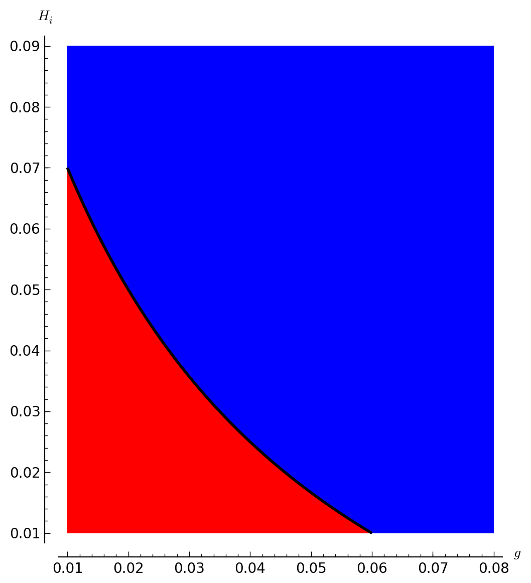
| (3) |
3.2 Well-Posed and Boundedness
For sake of simplicity, we denote
| (4) |
in such a way that the system (1) rewrites
| (5a) | |||
| (5b) | |||
| (5c) | |||
| (5d) | |||
We assume that all the coefficients presented in table 1 are all positive, that is:
| (6) |
The previous system of equations is written
| (7) |
The right-hand side of (7) is not properly defined in the points where . However, the following result demonstrates that this has no consequence on the solutions, as the latter stays away from this part of the subspace. For subsequent use, we denote the subset of those elements such that .
Theorem 1 (Well-posedness and boundedness).
If , then there exists a unique solution of (7) defined on such that . Moreover, for any , , and
| (8a) | |||
| (8b) | |||
where by definition , . Also,
| (9) |
and
| (10) |
Define as the largest set included in and fulfilling the inequalities of Theorem 1, that is:
| (11) |
Theorem 1 shows that the compact set is positively invariant and attracts all the trajectories. Therefore, in order to study the asymptotics of system (5), it is sufficient to consider the trajectories of (5) that are in .
3.3 Equilibria
Theorem 2 (Equilibria and asymptotic behavior).
Define
| (12) |
If , then there exists a unique equilibrium point of system (7) in , that corresponds to a mite-free situation. It is globally asymptotically stable, and given by
| (13) |
If , then there exists two equilibrium points in , namely and a coexistence equilibrium defined by
| (14) |
Moreover, for all initial conditions in except in a zero measure set, the trajectories tend towards .
Recall that , in such a way that
| (15) |
The point , that is , is the point of a transcritical bifurcation, that appears when gets larger than 1. For larger values, two equilibria are found analytically, a mite-free one, that is unstable, and a coexistence equilibrium which is stable. We’ve shown (Theorem 2) that the latter is globally asymptotically stable if , and conjecture that the same property holds for in the interval . Using as bifurcation parameter, the bifurcation appears for , after substituting the parameter values.
If we solve numerically the system from (5), we confirm the existence of two equilibria when crosses the bifurcation value of . The instability and stability of the mite-free and coexistence equilibria, respectively is shown in the simulation of figure 6.


4 Discussion and Conclusions
Coexistence of bees and Varroa mites in nature is an undeniable fact. However, this coexistence is fraught with dangers for the bees, since Varroa mites can be vectors of lethal viral diseases. These deleterious effects for the health of the individual workers and the whole colony, has led to the evolution of resistance behaviors such as the hygienic behavior and grooming.
Those behaviors are not entirely without cost to the bees, exacerbated hygienic behavior – when both and are intensified – can exert a substantial toll on the fitness of the queen. So it is safe to say that this parasitic relationship has evolved within a vary narrow range of parameters. Even if the mite-free equilibrium is advantageous to the colony, maintaining it may be too expensive to the bees.
[we need some discussion regarding the conditions for stability of , or the invasibility of the colony by mites]
On the other hand, in the absence of viral diseases, mite parasitism seems to be fairly harmless. If we look at the expression for the of infestation (3), we can see that the mite-induced bee mortality, , (not by viral diseases), must be kept low or risk destabilizing the co-existence equilibrium.
Africanized Honey bees, having evolved more effective resistance behaviors, are more resistant to CCD by their ability to keep infestation levels lower than those of their European counterparts(Moretto et al, 1991; Moretto et al, 1993). Unfortunately, the lack of more detailed experiments measuring the rates of grooming and higienic behaviors in both groups (EHB and AHB), makes it hard to position them accurately in the parameter space of the model presented.
Finally, we hope that the model presented here along with its demonstrated dynamical properties will serve as a solid foundation for the development of other models including viral dynamics and other aspects of bee colony health.
5 Appendix – Proofs of the theorems
Proof of Theorem 1.
Clearly, the right-hand side of the system of equations is globally Lipschitz on any subset of where is bounded away from zero. The existence and uniqueness of the solution of system (5) is then obtained for each trajectory staying at finite distance of this boundary. We will show that the two formulas provided in the statement are valid for each trajectory departing initially from a point where . As a consequence, the fact that all trajectories are defined on infinite horizon will ensue.
Summing up the first two equations in (5) yields, for any point inside :
| (16) |
Integrating this differential inequality between any two points and of a trajectory for which , , one gets
| (17) |
where the right-hand side is in any case positive for any .
Similarly, one has
| (18) |
and therefore
| (19) |
This proves in particular that the inequalities in (8a) hold for any portion of trajectory remaining inside .
We now consider the evolution of . Similarly to what was done for , one has
| (20) |
Therefore,
| (21) |
Integrating the lower bound of extracted from (17) yields the conclusion that any solution departing from indeed remains in as long as it is defined. On the other hand, we saw previously that trajectories remaining in could be extended on the whole semi-axis . Therefore, any trajectory departing from a point in can be extended to , and remains in for any . In particular, (8a) holds for any trajectory departing inside .
Let us now achieve the proof by bounding from above. One has
| (22) |
and thus
| (23) |
Using (19) then permits to achieve the proof of (8b), and finally the proof of (8).
Let us now prove (9). One deduces from (5a) and (5b) and the bounds established earlier the differential inequalities
| (24a) | |||
| (24b) | |||
The auxiliary linear time-invariant system
| (25) |
is monotone, as the state matrix involved is a Metzler matrix (?). Moreover, it is asymptotically stable, as the associated characteristic polynomial is equal to
| (26) |
and thus Hurwitz because . Therefore, all trajectories of (25) tend towards the unique equilibrium:
| (27) | |||||
Invoking Kamke’s Theorem, see e.g. (Coppel, 1965, Theorem 10, p. 29), one deduces from (24) and the monotony of (25) the following comparison result, that holds for all trajectories of (31):
| (28) |
This gives (9).
Proof of Theorem 2.
The proof is organized as follows.
- 1.
We first write system (5) under the form of an I/O system, namely
(30a) (30b) (30c) (30d) (30e) where , resp. , is the input, resp. the output, closed by the unitary feedback (30f) For subsequent use of the theory of monotone systems, one determines, for any (nonnegative) constant value of , the equilibrium values of for equation (30a)-(30d), and the corresponding values of as given by (30e).
- 2.
The equilibrium points of system (5) are then exactly (and easily) obtained by solving the fixed point problem among the solutions of the previous problem.
unique equilibrium points when , and there exist exactly two equilibrium points when . points.
- 3.
One then shows that the I/O system defined by (30a)-(30e) is anti-monotone with respect to certain order relation, and the study of the stability of these equilibria shows that it admits single-valued I/S and I/O characteristics, as in (Angeli and Sontag, 2004).
- 4.
Using this properties, the stability of the equilibria of the system obtained by closing the loop (30a)-(30e) by (30f) is then established using arguments similar to Angeli and Sontag (2003).
1. For fixed , the equilibrium equations of the I/O system (30) are given by
| (31a) | |||
| (31b) | |||
| (31c) | |||
| (31d) | |||
| (31e) | |||
Summing up the first and third identities gives
| (32) |
and thus necessarily:
| (33) |
The case yields , and then by (31a), and therefore has to be zero from (31b). Also, , by (31d), and then . in (11) and should be discarded. obtained point is located outside and has to be discarded; or
The case yields , and then by (31d) or (31c), and . There remains the two following conditions:
| (34) |
which yield
| (35) |
unconditionally.
Let us now look for possible values of in . From (33) and (31a)-(31c), one deduces
| (36) |
Using (33) on the one hand and summing the two identities (31b)-(31d) on the other hand, yields
| (37) |
This permits to express as a function of , namely:
| (38) |
Using this formula together with (33), (31d) and (36) now allows to find an equation involving only the unknown , namely:
| (39) |
Simplifying (as ) gives:
| (40) |
The previous condition is clearly affine in . It writes
| (41) |
which, after developing and simplifying, can be expressed as:
| (42) |
and finally
| (43) |
For , this equation admits a solution in if and only if
| (44) |
and the latter is given as
| (45) |
The state and output values may then be expressed explicitly as functions of . In particular, one has
| (46) |
(31) admits exactly one solution in for any ; admits a supplementary solution in for any . The following tables summarize the number of solutions of (31) for all nonnegative values of .
| Values of | Number of distinct solutions of (31) |
|---|---|
| 2 | |
| 1 |
| Values of | Number of distinct solutions of (31) |
|---|---|
| 3 | |
| 2 | |
| 1 |
2. The equilibrium points of system (5) are exactly those points for which for some nonnegative scalar , where is one of the output values corresponding to previously computed. We now examine in more details the solutions of this equation.
For the value in the previous computations, one should have , due to (45); but on the other hand for , due to (46). Therefore this point does not correspond to an equilibrium point of system (31).
The value yields a unique equilibrium point. Indeed, , so should be zero too, and the unique solution is given by
| (47) |
This corresponds to the equilibrium denoted in the statement.
Let us consider now the case of . For this case to be considered, it is necessary that , that is . The value of should be such that (see (46))
| (48) |
that is
| (49) |
or again
| (50) |
after replacing by its value defined in (12). The corresponding value of
| (51) |
given by (45), is clearly contained in when . Therefore, when , there also exists a second equilibrium. The latter is given by:
| (52a) | |||
| (52b) | |||
| (52c) | |||
and corresponds to defined in the statement.
diagonal that comes from the loop closing.
3. Let be the cone in defined as the product of orthants . We endow the state space with this order. In other words, for any and in , means:
| (53) |
With this structure, one may verify that the system (30a)-(30e) has the following monotonicity properties (Hirsch, 1988; Smith, 2008)
- •
For any function locally integrable and taking on positive values almost everywhere, for any ,
(54) where by definition denotes the value at time of the point in the trajectory departing at time from and subject to input .
- •
The Jacobian matrix of the I/O system is
(55) which is irreducible when and . The system is therefore strongly monotone in (notice that does not contain points for which ), and also on the invariant subset .
- •
The input-to-state map is monotone, that is: for any inputs , for any ,
(56) - •
The state-to-output map is anti-monotone, that is: for any ,
(57)
monotone (due to the irreducibility of the Jacobian matrix) for any constant value of .
In order to construct I/S and I/O characteristics for system (31), we now examine the stability of the equilibria of system (31) for any fixed value of . As shown by Theorem 1, all trajectories are precompact.
When , it has been previously established that for any there exists at most one equilibrium in to the I/O system (31). The strong monotonicity property of this system depicted above then implies that this equilibrium is globally attractive (Hirsch, 1988, Theorem 10.3). Therefore, system (31) possesses I/S and I/O characteristics. As for any value of , this equilibrium corresponds to zero output, the I/O characteristics is zero. Applying the results of Angeli and Sontag (2004), one gets that the closed-loop system equilibrium is an almost globally attracting equilibrium for system (5).
Let us now consider the case where . We first show that the equilibrium point with and (34) is locally unstable. Notice that this point is located on a branch of solution parametrized by and departing from for . The Jacobian matrix (55) taken at this point is
| (58) |
This matrix is block triangular, with diagonal blocks
| (59) |
The first of them is clearly Hurwitz, while the second, whose characteristic polynomial is
| (60) |
(where is defined in (44)) is not Hurwitz when and , and has a positive root for . Therefore, the corresponding equilibrium of the I/O system (30) is unstable for these values of .
The other solution, given as a function of by (52), is located on a branch of solution parametrized by and departing from for . As the other solution is unstable for , one can deduce from Hirsch (1988, Theorem 10.3) that these solutions are locally asymptotically stable.
One may now associate to any the corresponding unique locally asymptotically stable equilibrium point, and the corresponding output value, defining therefore respectively an I/S characteristic and an I/O characteristic for system (30).
For any scalar , for almost any , one has
| (61) |
and, from the monotony properties, for any scalar-valued continuous function , for almost any :
| (62) |
Using the fact that is anti-monotone and that for the closed-loop system, one deduces, as e.g. in Gouzé (1988) that, for the solutions of the latter,
| (63) |
Here , defined by (46), is a linear decreasing map. When its slope is smaller than 1, then the sequences in the left and right of (63) tend towards the fixed point that corresponds to the output value at , see (50).
This slope value, see (46), is equal to
| (64) |
and it thus smaller than 1 if and only if , which is an hypothesis of the statement.
Acknowledgements.
The authors would like to thank Fundação Getulio Vargas for financial support in the form of a scholarship to Joyce de Figueiró Santos. They are also grateful for valuable comments by Moacyr A. H. Silva, Max O. Souza and Jair Koiler on an early version of the manuscript.Compliance with Ethical Standards
Conflict of Interest: The authors declare that they have no conflict of interest.
References
- Angeli and Sontag (2004) Angeli D, Sontag E (2004) Interconnections of monotone systems with steady-state characteristics. In: Optimal control, stabilization and nonsmooth analysis, Springer, pp 135–154
- Angeli and Sontag (2003) Angeli D, Sontag ED (2003) Monotone control systems. Automatic Control, IEEE Transactions on 48(10):1684–1698
- Arechavaleta-Velasco and Guzman-Novoa (2001) Arechavaleta-Velasco ME, Guzman-Novoa E (2001) Relative effect of four characteristics that restrain the population growth of the mite Varroa destructor in honey bee ( Apis mellifera ) colonies. Apidologie 32(2):157–174, DOI 10.1051/apido:2001121, URL http://www.apidologie.org/index.php?option=com_article&access=standard&Itemid=129&url=/articles/apido/pdf/2001/02/velasco.pdf, 00000
- Calderón et al (2010) Calderón RA, Veen JWv, Sommeijer MJ, Sanchez LA (2010) Reproductive biology of varroa destructor in africanized honey bees (apis mellifera). Experimental and Applied Acarology 50(4):281–297, DOI 10.1007/s10493-009-9325-4, URL http://link.springer.com/article/10.1007/s10493-009-9325-4, 00010
- Carneiro et al (2007) Carneiro FE, Torres RR, Strapazzon R, Ramírez SA, Guerra Jr JCV, Koling DF, Moretto G (2007) Changes in the reproductive ability of the mite varroa destructor (anderson e trueman) in africanized honey bees (apis mellifera l.) (hymenoptera: Apidae) colonies in southern brazil. Neotropical Entomology 36(6):949–952, DOI 10.1590/S1519-566X2007000600018, URL http://www.scielo.br/scielo.php?pid=S1519-566X2007000600018&script=sci_arttext, 00022
- Coppel (1965) Coppel WA (1965) Stability and asymptotic behavior of differential equations, vol 11. Heath Boston
- Corrêa-Marques et al (1998) Corrêa-Marques MH, David DE, others (1998) Uncapping of worker bee brood, a component of the hygienic behavior of africanized honey bees against the mite varroa jacobsoni oudemans. Apidologie 29(3):283–289, URL http://hal.archives-ouvertes.fr/docs/00/89/14/94/PDF/hal-00891494.pdf
- Van den Driessche and Watmough (2002) Van den Driessche P, Watmough J (2002) Reproduction numbers and sub-threshold endemic equilibria for compartmental models of disease transmission. Mathematical biosciences 180(1):29–48, URL http://www.sciencedirect.com/science/article/pii/S0025556402001086
- Gouzé (1988) Gouzé JL (1988) A criterion of global convergence to equilibrium for differential systems. Application to Lotka-Volterra systems. Research Report RR-0894, URL https://hal.inria.fr/inria-00075661
- Hirsch (1988) Hirsch MW (1988) Stability and convergence in strongly monotone dynamical systems. J reine angew Math 383(1):53
- Khoury et al (2011) Khoury DS, Myerscough MR, Barron AB (2011) A quantitative model of honey bee colony population dynamics. PLoS ONE 6(4):e18,491, DOI 10.1371/journal.pone.0018491, URL http://dx.doi.org/10.1371/journal.pone.0018491
- Medina and Martin (1999) Medina LM, Martin SJ (1999) A comparative study of varroa jacobsoni reproduction in worker cells of honey bees (apis mellifera) in england and africanized bees in yucatan, mexico. Experimental & Applied Acarology 23(8):659–667, DOI 10.1023/A:1006275525463, URL http://link.springer.com/article/10.1023/A%3A1006275525463
- Mondragón et al (2005) Mondragón L, Spivak M, Vandame R (2005) A multifactorial study of the resistance of honeybees Apis mellifera to the mite Varroa destructor over one year in mexico. Apidologie 36(3):345–358, DOI 10.1051/apido:2005022, URL http://www.apidologie.org/index.php?option=com_article&access=standard&Itemid=129&url=/articles/apido/pdf/2005/03/M4080.pdf, 00000
- Moretto et al (1991) Moretto G, Gonçalves LS, De Jong D, Bichuette MZ, others (1991) The effects of climate and bee race on varroa jacobsoni oud infestations in brazil. Apidologie 22(3):197–203, URL http://hal.archives-ouvertes.fr/docs/00/89/09/07/PDF/hal-00890907.pdf
- Moretto et al (1993) Moretto G, Gonçalves LS, De Jong D (1993) Heritability of africanized and european honey bee defensive behavior against the mite varroa jacobsoni. Revista Brasileira de Genetica 16:71–71
- Oldroyd (2007) Oldroyd BP (2007) What’s killing american honey bees? PLoS Biol 5(6):e168, DOI 10.1371/journal.pbio.0050168, URL http://dx.doi.org/10.1371/journal.pbio.0050168, 00205
- Pereira et al (2002) Pereira FdM, Lopes MTR, Camargo RCR, Vilela SLO (2002) Organização social e desenvolvimento das abelhas apis mellifera. URL http://sistemasdeproducao.cnptia.embrapa.br/FontesHTML/Mel/SPMel/organizacao.htm
- Pinto et al (2012) Pinto FA, Puker A, Barreto LMRC, Message D (2012) The ectoparasite mite varroa destructor anderson and trueman in southeastern brazil apiaries: effects of the hygienic behavior of africanized honey bees on infestation rates. Arquivo Brasileiro de Medicina Veterinária e Zootecnia 64(5):1194–1199, DOI 10.1590/S0102-09352012000500017, URL http://www.scielo.br/scielo.php?script=sci_abstract&pid=S0102-09352012000500017&lng=en&nrm=iso&tlng=en
- Ratti et al (2012) Ratti V, Kevan PG, Eberl HJ (2012) A mathematical model for population dynamics in honeybee colonies infested with varroa destructor and the acute bee paralysis virus. Canadian Applied Mathematics Quarterly
- Smith (2008) Smith HL (2008) Monotone dynamical systems: an introduction to the theory of competitive and cooperative systems, vol 41. American Mathematical Soc.
- Spivak (1996) Spivak M (1996) Honey bee hygienic behavior and defense against varroa jacobsoni. Apidologie 27:245–260, URL http://www.apidologie.org/index.php?option=com_article&access=standard&Itemid=129&url=/articles/apido/pdf/1996/04/Apidologie_0044-8435_1996_27_4_ART0007.pdf
- Vandame et al (2000) Vandame R, Colin ME, Morand S, Otero-Colina G (2000) Levels of compatibility in a new host-parasite association: Apis mellifera/Varroa jacobsoni. Canadian Journal of Zoology 78(11):2037–2044, DOI 10.1139/z00-109, URL http://www.nrcresearchpress.com/doi/abs/10.1139/z00-109, 00023
- Vandame et al (2002) Vandame R, Morand S, Colin ME, Belzunces LP (2002) Parasitism in the social bee Apis mellifera : quantifying costs and benefits of behavioral resistance to Varroa destructor mites. Apidologie 33(5):433–445, DOI 10.1051/apido:2002025, URL http://www.apidologie.org/index.php?Itemid=129&option=com_article&access=doi&doi=10.1051/apido:2002025&type=pdf, 00000