Accuracy of spike-train Fourier reconstruction for colliding nodes

Andrey Akinshin¹, Dmitry Batenkov², Yosef Yomdin³ Affiliation: ¹³Department of Mathematics,
The Weizmann Institute of Science, Rehovot 76100, Israel Affiliation: ¹Laboratory of Inverse Problems of Mathematical Physics,
Sobolev Institute of Mathematics SB RAS, Novosibirsk 630090, Russia Affiliation: ²Department of Computer Science,
Technion — Israel Institute of Technology, Haifa 32000, Israel Affiliation: ¹ Email: andrey.akinshin@weizmann.ac.il Affiliation: ² Email: yosef.yomdin@weizmann.ac.il Affiliation: ³ Email: batenkov@cs.technion.ac.il

Abstract

We consider signal reconstruction problem for signals $F$ of the form $F(x)=\left(x\right)=\sum_{j=1}^{d}a_{j}\delta\left(x-x_{j}\right),$ from their Fourier transform ${\cal F}(F)(s)=\int_{-\infty}^{\infty}F(x)e^{-isx}dx.$ We assume ${\cal F}(F)(s)$ to be known for each $s\in[-N,N],$ with an absolute error not exceeding $\epsilon>0$ . We give an absolute lower bound (which is valid with any reconstruction method) for the “worst case” error of reconstruction of $F$ from ${\cal F}(F),$ in situations where the nodes $x_{j}$ are known to form an $l$ elements cluster of a size $h\ll 1$ . Using “decimation” algorithm of [7, 6] we provide an upper bound for the reconstruction error, essentially of the same form as the lower one. Roughly, our main result states that for $h$ of order $\frac{1}{N}\epsilon^{\frac{1}{2l-1}}$ the worst case reconstruction error of the cluster nodes is of the same order $\frac{1}{N}\epsilon^{\frac{1}{2l-1}}$ , and hence the inside configuration of the cluster nodes (in the worst case scenario) cannot be reconstructed at all. On the other hand, decimation algorithm reconstructs $F$ with the accuracy of order $\frac{1}{N}\epsilon^{\frac{1}{2l}}$ .

I Introduction

In this paper, we provide lower and upper bounds for the Fourier reconstruction error, in the presence of noise, of spike-train signals in the case of “almost colliding” (or clustering) nodes. The lower bound is obtained via the analysis of the behavior of the Fourier transform under perturbation of the nodes and amplitudes in the cluster, and so it is valid (in the worst case scenario) for any reconstruction method. The upper bound follows from the accuracy analysis of “decimation” reconstruction algorithm, as given in [7, 6].

We hope that our analysis may clarify some aspects of the “Super-resolution problem” for spike-train signals with clustering nodes, as it appears in many old and recent publications on the subject (see, as a very small sample, [13, 12, 17, 19, 23, 20], recent publications [1, 7, 6, 2, 4, 5, 9, 8, 11, 15, 16, 18, 21, 10, 22, 3, 14, 26], and references therein).

Let us assume that the signal $F(x)$ is a spike-train, i.e. it is a priori known to be a linear combination of $d$ shifted $\delta$ -functions:

F(x)=F_{A,X}\left(x\right)=\sum_{j=1}^{d}a_{j}\delta\left(x-x_{j}\right),

(1)

where $A=(a_{1},\ldots,a_{d})\in{\mathbb{R}}^{d},\ X=X_{d}=(x_{1},\ldots,x_{d})\in{\mathbb{R}}^{d}.$ We shall always assume that $x_{1}\leq x_{2}\leq\ldots\leq x_{d}$ . As for the measurements, we assume that the Fourier transform

{\cal F}(F)(s)=\int_{-\infty}^{\infty}F(x)e^{-isx}dx

(2)

is known for each $s\in[-N,N],$ with an absolute error not exceeding $\epsilon>0$ . So our input measurement is a function $\Phi(s)$ satisfying $|\Phi(s)-{\cal F}(F)(s)|\leq\epsilon$ for $s\in[-N,N]$ .

The first goal of the present paper is to study the “worst case” accuracy of reconstruction of $F$ from $\Phi(s)$ in situations where the nodes $x_{j}$ are known to form a cluster of a size $h\ll 1$ , while being near-uniformly positioned inside the cluster. We give an absolute lower bound for the reconstruction error of the nodes $x_{j}$ from the measured function $\Phi(s),$ which is valid independently of the reconstruction method applied.

Our second goal is to give an upper bound for the reconstruction error of the nodes $x_{j}$ , under the same assumptions as above. We show that the decimation algorithm, combined with a homotopy continuation solving of the resulting algebraic equations, as described in [7, 6], produces an error of essentially the same order of magnitude as the lower bound.

Shortly, our main result is as follows:

1. If certain $l$ nodes of $F$ form a cluster of a size $h\sim\frac{1}{N}\epsilon^{\frac{1}{2l-1}}$ , while being near-uniformly positioned inside the cluster, then the worst case reconstruction error $\Delta$ of the cluster nodes is at least $Ch$ .

2. If for the same signal $F$ the measurements error is smaller than $\epsilon_{1}\sim\epsilon^{\frac{2l}{2l-1}}$ then the decimation algorithm reconstructs the cluster nodes with the error $\Delta$ being at most $ch,\ c\ll C.$

The “practical” conclusion could be that the inside configuration of the cluster nodes cannot be reconstructed at all from the Fourier transform ${\cal F}(F)(s),$ known with the error $\epsilon,$ for $s\in[-N,N],$ if the cluster size $h$ is smaller than $\frac{1}{N}\epsilon^{\frac{1}{2l-1}}$ . However, slightly reducing (to $\epsilon_{1}$ ) the allowed magnitude of the measurements error, we can accurately and robustly reconstruct the cluster nodes via the decimation algorithm.

The reconstruction error $\Delta\sim\frac{1}{N}\epsilon^{\frac{1}{2l-1}}$ would make practical reconstruction of two colliding nodes very difficult, and of three or more virtually impossible. However, our bound is the worst case one, and one can hope that for a random noise a typical reconstruction accuracy may be much better.

Let us stress that our result is pretty close to the main result of [13], where Fourier sampling of atomic measures on non-uniform grids is studied. In particular, the connection of the form $\epsilon=C(Nh)^{2l-1}$ between the noise, the bandwidth, and the clustering geometry which can be stably recovered, appears also in [13]. Very recently similar bounds were obtained for superresolution of positive sources in [22], and for a Fourier recovery of sparse vectors in [10]. There are also apparent similarities with the classical result of Slepian in [24]. Compare a discussion in [9] of the role of sparsity and clustering, as they appear in the superresolution problem, and, in particular, the discussion in Sections 1.7 and 3.2 of [9] of the “absolute lower bounds” for the reconstruction error. We plan to further investigate the above connections.

II Main result

To state our results we have to make some “normalizing” assumptions on the signal $F$ to be recovered. Indeed, if some amplitudes $a_{j}$ are small, the reconstruction accuracy of the corresponding nodes drops, while larger $a_{j}$ imply higher accuracy. So we shall assume that the amplitudes $A=(a_{1},\ldots,a_{d})$ of the signal $F$ satisfy the following assumption $A(m,M)$ :

0<m\leq|a_{j}|\leq M<\infty,\ j=1,\ldots,d.

Definition II.1

A signal $F_{A,X}$ as given by (1) is said to form an $(l,h,\rho)$ -cluster $X$ if there is an interval $I\subset{\mathbb{R}}$ of length $h$ which contains exactly $l$ nodes $X_{l}=\{x_{\kappa},x_{\kappa+1},\ldots,x_{\kappa+l-1}\}$ of $F$ , while the minimal distance between the nodes in $X_{l}$ is at least $\rho h$ , $\rho>0$ .

Definition II.2

For two ordered subsets $V=(v_{1},\ldots,v_{q})$ , and $W=(w_{1},\ldots,w_{q})$ in ${\mathbb{R}}$ the distance $d(V,W)$ is defined as

d(V,W)={\rm max\,}_{s=1}^{q}|v_{s}-w_{s}|=||v_{s}-w_{s}||_{l^{\infty}}\geq\\ \geq\frac{1}{\sqrt{q}}||v_{s}-w_{s}||_{l^{2}}.

The following theorem is the first main result of the paper:

Theorem II.1

Let a signal $F^{0}=F_{A^{0},X^{0}},$ satisfying assumption $A(m,M)$ , form an $(l,h,\rho)$ -cluster $X^{0}_{l}=\{x^{0}_{\kappa},x^{0}_{\kappa+1},\ldots,x^{0}_{\kappa+l-1}\}.$ Then there exist parameters $A^{1},X^{1}$ , satisfying assumption $A(\frac{m}{2},2M)$ , such that the distance $d(X^{0}_{l},X^{1}_{l})$ between $X^{0}_{l}$ and $X^{1}_{l}=\{x^{1}_{\kappa},x^{1}_{\kappa+1},\ldots,x^{1}_{\kappa+l-1}\}$ is at least $C_{1}h$ , while for $F^{1}=F_{A^{1},X^{1}},$ and for each $s\in{\mathbb{R}}$ with $|s|\leq\frac{1}{2\pi h}$ we have

|{\cal F}(F^{0})(s)-{\cal F}(F^{1})(s)|\leq C_{2}(hs)^{2l-1}.

(3)

In particular, for $s\in[-N,N],\ N\leq\frac{1}{2\pi h},$ this difference does not exceed $C_{2}(hN)^{2l-1}.$ Here the constants $C_{1}$ and $C_{2}$ depend only on $m,M,l,\rho.$

The proof of Theorem II.1 is given in Section III below. From this result we immediately deduce the following:

Corollary II.1

Assume that the noise $N(s)$ in the Fourier sampling ${\cal F}(s)$ on $[-N,N]$ may be an arbitrary function with the only restriction that $|N(s)|\leq\epsilon,$ where $0<\epsilon\ll 1$ , and put $h_{\epsilon}=\frac{1}{N}(\frac{\epsilon}{C_{2}})^{\frac{1}{2l-1}}.$ Let $F^{0}$ be any signal, satisfying assumption $A(m,M)$ , and forming an $(l,h_{\epsilon},\rho)$ -cluster $X^{0}_{l}$ . Let $F^{1}$ be the new signal produced from $F^{0}$ as in Theorem II.1. Then for any reconstruction algorithm $\cal R$ the worst-case error in reconstruction of the nodes of either $X^{0}_{l}$ , or of $X^{1}_{l}$ is not smaller than $\frac{1}{2}C_{1}h_{\epsilon}$ .

Proof: We pick an “adversary” noise $N(s)$ to be identically zero for the sampling of $F^{0}$ and to be equal to $N(s)={\cal F}(F^{0})(s)-{\cal F}(F^{1})(s)$ for the sampling of $F^{1}$ In both cases, by our choice of $h_{\epsilon}$ and by Theorem II.1, we have $|N(s)|\leq\epsilon,\ s\in[-N,N]$ . Notice that for sufficiently small $\epsilon$ we have $h_{\epsilon}\ll{1\over N}$ , and hence the condition $N\leq\frac{1}{2\pi h}$ of Theorem II.1 is satisfied. The measurement results $\Phi(s)$ are identical for $F^{0}$ and $F^{1}$ , and whatever reconstruction $(\hat{A},\hat{X})$ of the signal parameters the algorithm $\cal R$ produces from $\Phi(s)$ , either the distance $d(X^{0}_{l},\hat{X}_{l}),$ or $d(X^{1}_{l},\hat{X}_{l}),$ is at least $\frac{1}{2}d(X^{0}_{l},X^{1}_{l})$ which, by Theorem II.1, is not smaller than $\frac{1}{2}C_{1}h_{\epsilon}$ . $\square$

As for the upper bound on the reconstruction error, we announce the following result:

Theorem II.2

Let a signal $F^{0}=F_{A^{0},X^{0}},$ satisfying assumption $A(m,M)$ , form an $(l,h,\rho)$ -cluster $X^{0}_{l}=\{x^{0}_{\kappa},x^{0}_{\kappa+1},\ldots,x^{0}_{\kappa+l-1}\}.$ Let the measurements error $\epsilon$ satisfy $\epsilon\leq\epsilon_{1}=C_{3}(hN)^{2l}.$ Then solving the corresponding decimated Prony system of [6] produces the reconstructed cluster nodes $\bar{X}^{0}_{l}$ with the error at most $\frac{1}{10}\rho h$ , i.e. $d(X^{0},\bar{X}^{0})\leq\frac{1}{10}\rho h$ .

In particular, since by the assumptions the distance between the cluster nodes is at least $\rho h,$ the number of the nodes, and the inner geometry of the cluster can be robustly restored.

The proof of Theorem II.2 is based on a combination of the Jacobian estimates in [7, 6] with the “Quantitative Inverse Function theorem” (Theorem III.2 below). We plan to present the details separately.

III Proof of Theorem II.1

We prove Theorem II.1 in several steps. First, for signals $F$ as above we express the Fourier transform ${\cal F}(F)$ through the moments $m_{k}(F)$ .

III-A Fourier transform ${\cal F}(F)$ and moments $m_{k}(F)$

For signals $F$ of form (1) their Fourier transform ${\cal F}(F)$ can be easily computed explicitly. Let the moments $m_{k}(F)$ be defined by

\begin{array}[]{c}m_{k}(F_{A,X})=\int_{-\infty}^{\infty}x^{k}F_{A,X}(x)dx=\\ =\sum_{j=1}^{d}a_{j}x_{j}^{k},\ k=0,1,\ldots.\end{array}

(1)

Proposition III.1

For $F=F_{A,X}=\sum_{j=1}^{d}a_{j}\delta(x-x_{j})$ we have

{\cal F}(F)(s)=\sum_{k=0}^{\infty}{{m_{k}(F)}\over{k!}}\tilde{s}^{k},\ \text{w}here\ \ \tilde{s}=-2\pi is.

(2)

Proof:

\begin{array}[]{c}{\cal F}(F)(s)=\int_{-\infty}^{\infty}e^{-2\pi isx}F(x)dx=\sum_{j=1}^{d}a_{j}e^{-2\pi ix_{j}s}=\\ =\sum_{j=1}^{d}a_{j}\sum_{k=0}^{\infty}{1\over{k!}}(-2\pi ix_{j}s)^{k}=\\ =\sum_{k=0}^{\infty}{1\over{k!}}(-2\pi is)^{k}\sum_{j=1}^{d}a_{j}x_{j}^{k}=\\ =\sum_{k=0}^{\infty}{1\over{k!}}m_{k}(F)\tilde{s}^{k}.\ \ \square\end{array}

Thus the Taylor coefficients of the Fourier transform ${\cal F}(F)(s)$ are the consecutive moments $m_{k}(F)$ divided by $k!$ This fact provides us an “Algebraic-Geometric” approach to the Fourier reconstruction: to produce the signal $F^{1}$ starting with $F^{0}$ we analyze the behavior of the moments $m_{k}(F)$ , and keep them the same for $F^{0}$ and $F^{1}$ for $k=0,1,\ldots,2l-2.$ This analysis strongly relies on recent results in [7, 4, 5] on the geometry of the “Prony mapping”, which is formed by the moments $m_{k}(F)$ .

III-B Reduction of Theorem II.1 to a geometric lemma

The following result is proved in Section III-C below:

Lemma III.1

Let a signal $F^{0}=F_{A^{0},X^{0}},$ satisfying assumption $A(m,M)$ , form an $(d,1,\rho)$ -cluster $X^{0}=\{x^{0}_{1},\ldots,x^{0}_{d}\}.$ In other words, all the $d$ nodes of $F^{0}$ are $\rho$ -uniformly distributed in the interval $[-\frac{1}{2},\frac{1}{2}]$ . Then there exist parameters $A^{1},X^{1}$ , satisfying assumption $A(\frac{m}{2},2M)$ , with $X^{1}=(x^{1}_{1},\ldots,x^{1}_{d})\subset[-1,1]$ , such that

1. The distance $d(X^{0},X^{1})$ between the nodes sets $X^{0}$ and $X^{1}$ is at least $C_{1}(m,M,d)>0.$

2. $m_{k}(F^{0})=m_{k}(F^{1}),\ k=0,1,\ldots,2d-2,$ where $F_{1}=F_{A^{1},X^{1}}$ .

Now we can complete the proof of Theorem II.1. Let a signal $F^{0}=F_{A^{0},X^{0}},$ satisfying assumption $A(m,M)$ , form an $(l,h,\rho)$ -cluster $X^{0}_{l}=(x^{0}_{\kappa},x^{0}_{\kappa+1},\ldots,x^{0}_{\kappa+l-1}).$ We rescale the cluster $X^{0}_{l}$ to $X^{\prime 0}_{l}$ in the interval $[-\frac{1}{2},\frac{1}{2}]$ , with the same amplitudes $A^{0}_{l}$ . Then we apply Lemma III.1 (where we put $d=l$ ), and find the amplitudes $A^{1}_{l}$ and the nodes $X^{\prime 1}_{l}$ in the interval $[-1,1]$ , with the same moments as $X^{\prime 0}_{l}$ up to $2l-2$ . Applying the inverse scaling, and obtain the cluster $X^{1}_{l}\subset[-h,h]$ . Clearly, if the moments were equal before shrinking, they will remain equal afterwards. We extend the cluster $X^{1}_{l}$ with the amplitudes $A^{1}_{l}$ to the required parameters $A^{1},X^{1}$ , adding the non-cluster nodes of $X^{0}$ with their original amplitudes. By Lemma III.1 the distance $d(X^{0}_{l},X^{1}_{l})$ is at least $C_{1}h,$ while $m_{k}(F^{0})=m_{k}(F^{1}),\ k=0,1,\ldots,2l-2.$

It remains to show that $|{\cal F}(F_{A,X})(s)-{\cal F}(F_{\bar{A},\bar{X}})(s)|\leq C_{2}(hs)^{2l-1}.$ By Proposition III.1 we have

{\cal F}(F_{A,X})(s)-{\cal F}(F_{\bar{A},\bar{X}})(s)=\sum_{k=0}^{\infty}\frac{\gamma_{k}}{k!}\tilde{s}^{k},

(3)

where $\gamma_{k}=m_{k}(F_{A,X})-m_{k}(F_{\bar{A},\bar{X}}),$ and $\tilde{s}=-2\pi is.$ But by our construction $\gamma_{k}=0,\ k=0,1,\ldots,2l-2.$ On the other hand, since both $X_{l}$ and $\bar{X}_{l}$ are inside $[-h,h]$ , while the amplitudes are bounded by $2M,$ we have for any $k$ that $|\gamma_{k}|\leq 4lMh^{k}:=C_{3}h^{k}.$ So in fact, for $|s|\leq\frac{1}{2\pi h}$ we get

\begin{array}[]{c}\displaystyle|{\cal F}(F_{A,X})(s)-{\cal F}(F_{\bar{A},\bar{X}})(s)|\leq\sum_{k=2l-1}^{\infty}\frac{C_{3}}{k!}|\tilde{s}h|^{k}\leq\\ \displaystyle\leq C_{3}(2\pi sh)^{2l-1}\sum_{q=0}^{\infty}\frac{1}{(2l-1+q)!}(2\pi sh)^{q}\leq\\ \displaystyle\leq\frac{2C_{3}(2\pi)^{2l-1}}{(2l-1)!}(sh)^{2l-1}=C_{2}(sh)^{2l-1},\end{array}

where we put $C_{2}=\frac{2C_{3}(2\pi)^{2l-1}}{(2l-1)!}$ . This completes the proof of Theorem II.1. $\square$

III-C Proof of Lemma III.1

Let a signal $F^{0}=F_{A^{0},X^{0}},$ satisfying assumption $A(m,M)$ , be given, such that all the $d$ nodes of $F$ are $\rho$ -uniformly distributed in the interval $[-\frac{1}{2},\frac{1}{2}]$ . We have to show that there exist parameters $A^{1},X^{1}$ , satisfying assumption $A(\frac{m}{2},2M)$ , with $X^{1}_{d}=(x^{1}_{1},\ldots,x^{1}_{d})\subset[-1,1]$ , such that the system of equations

\begin{array}[]{c}m_{k}(F^{0})=m_{k}(F^{1}),\ F^{1}=F_{A^{1},X^{1}},\\ k=0,1,\ldots,2d-2\end{array}

(4)

is satisfied, while the distance $d(X^{0}_{d},X^{1}_{d})$ is at least $C_{1}(m,M,d)>0.$ In other words, we have to show that the projection of the set $Q\subset{\mathbb{R}}^{d}\times{\mathbb{R}}^{d}$ consisting of $A^{1},X^{1}$ which satisfy (4), is large enough.

Let us recall a definition of the Prony mapping $PM:{\mathbb{R}}^{d}\times{\mathbb{R}}^{d}\to{\mathbb{R}}^{2d}$ , given in [5]. It is provided by

PM(A,X)=\left(m_{0}(F_{A,X}),\ldots,m_{2d-1}(F_{A,X})\right)\in{\mathbb{R}}^{2d}.

(5)

Put $m^{0}_{k}=m_{k}(F_{A,X}).$ Then $PM(A^{0},X^{0})=(m^{0}_{0},m^{0}_{1},\ldots,m^{0}_{2d-1}).$ We shall denote by

\begin{array}[]{c}\mu=(\mu_{0},\ldots,\mu_{2d-1})=\\ =(m_{0}-m^{0}_{0},\ m_{1}-m^{0}_{1},\ \ldots,\ m_{2d-1}-m^{0}_{2d-1})\end{array}

the coordinates in ${\mathbb{R}}^{2d}$ , with the origin shifted to $\mu^{0}=PM(A^{0},X^{0})$ . The following result can be easily derived from Theorem 4.5 of [4]:

Theorem III.1

At each point $(A^{0},X^{0})\in{\mathbb{R}}^{d}\times{\mathbb{R}}^{d}$ satisfying conditions of Lemma III.1, the Jacobian $JPM=JPM(A^{0},X^{0})$ of the Prony mapping $PM$ is invertible, the norm of its inverse $JPM^{-1}$ is bounded from above by the constant $C_{5}(m,M,d,\rho)$ , and for each $\mu\in{\mathbb{C}}^{2d}$ we have $||JPM^{-1}(\mu)||\geq C_{6}||\mu||,$ with a positive $C_{6}=C_{6}(m,M,d,\rho).$

Let $L=O\mu_{2d-1}$ be the last coordinate axis in ${\mathbb{R}}^{2d}$ , and let

P_{X}:{\mathbb{R}}^{d}\times{\mathbb{R}}^{d}\to{\mathbb{R}}^{d}

denote the projection of the signal parameters $A,X$ to the nodes coordinates $X$ . Then for each $\mu\in L$ we have $||P\circ JPM^{-1}(\mu)||\geq C_{7}||\mu||,$ with a positive $C_{7}=C_{7}(m,M,d,\rho).$

Proof: The first three statements of Theorem III.1 follow directly from Theorem 4.5 of [4]. The last statement follows from the fact that for the fixed nodes the restriction of the first $d$ coordinates of the Prony mapping $PM$ , and hence, of its Jacobian $JPM$ , to the coefficients $A$ is a non-degenerate linear mapping to ${\mathbb{R}}^{d}$ , with the Vandermonde matrix on the nodes $X$ . Hence, the pre-image $JPM^{-1}(L)$ cannot be contained in ${\mathbb{R}}^{d}\times\{0\}\subset{\mathbb{R}}^{d}\times{\mathbb{R}}^{d}$ . Otherwise at least one of the first $d$ moments would change along $L$ . In fact, it is easy to show that the line $JPM^{-1}(L)$ forms a positive angle with ${\mathbb{R}}^{d}\times\{0\}$ , which is bounded from below by a constant depending only on $m,M,d,\rho$ . But this is equivalent to the last statement of Theorem III.1. $\square$

On the other hand, using the standard solution procedure of the Prony system, one can easily show the following fact:

Proposition III.2

There are constants $R_{1}=R_{1}(m,M,d,\rho)$ and $C_{8}=C_{8}(m,M,d,\rho),$ such that for each point $(A^{0},X^{0})\in{\mathbb{R}}^{d}\times{\mathbb{R}}^{d}$ , satisfying conditions of Lemma III.1, the first and the second derivatives of the Prony mapping $PM$ are bounded by $C_{8}$ in the ball $B_{R_{1}}$ in ${\mathbb{R}}^{d}\times{\mathbb{R}}^{d}$ centered at $(A^{0},X^{0})$ .

With these two preparatory results we now apply the following “Quantitative Inverse Function Theorem” (see. e.g. [25]):

Theorem III.2

Let $G:(B^{m}_{1},0)\to({\mathbb{R}}^{m},0)$ be a twice differentiable mapping of the unit ball $B^{m}_{1}$ at the origin in ${\mathbb{R}}^{m}$ to ${\mathbb{R}}^{m}$ , with $G(0)=0$ , such that the Jacobian $J=JG(0)$ is invertible, and $||J^{-1}||\leq K_{1}<\infty.$ Assume that the second derivatives of $G$ are bounded by $K_{2}$ in the ball $B^{m}_{1}.$ Then the inverse mapping $G^{-1}$ exists in the ball $B^{m}_{R_{2}}$ of radius $R_{2}$ , centered at $0\in{\mathbb{R}}^{m}$ , and satisfies there the condition

\begin{array}[]{c}||G^{-1}(x)-J^{-1}(x)||\leq C_{9}(m,K_{1},K_{2})||x||^{2},\\ \text{f}or\ \ x\in B^{m}_{R_{2}},\end{array}

(6)

with $R_{2}=R_{2}(m,K_{1},K_{2})$ and $C_{9}=C_{9}(m,K_{1},K_{2})$ depending only on $m,K_{1},$ and $K_{2}$ .

We apply Theorem III.2, properly rescaled, to the the Prony mapping $PM$ in the ball $B_{R_{1}}$ in ${\mathbb{R}}^{d}\times{\mathbb{R}}^{d}$ centered at $(A^{0},X^{0})$ , with the bounds provided by Theorem III.1 and Proposition III.2. We conclude that in the ball $B_{R_{3}}$ of radius $R_{3}$ at the point $\mu^{0}=PM(A^{0},X^{0})\in{\mathbb{R}}^{2d}$ the inverse $PM^{-1}$ exists and satisfies

||PM^{-1}(\mu)-J^{-1}(\mu)||\leq C_{10}||\mu||^{2},

(7)

where $J=JPM$ is the Jacobian of the Prony mapping $PM$ at $(A^{0},X^{0})$ , and the constants $R_{3}$ and $C_{10}$ depend only on $m,M,d,\rho$ .

From the last statement of Theorem III.1 we get for $\mu\in L=O\mu_{2d-1}$

||P\circ J^{-1}(\mu)||\geq C_{11}||\mu||,

(8)

with $P$ the projection of the signal parameters $A,X$ to the nodes $X$ , and $C_{11}=C_{11}(m,M,d,\rho)$ a positive constant.

Finally we put $\mu^{1}=(0,\ldots,0,\eta)$ , with $\eta={\rm min\,}\bigl(R_{3},\frac{C_{11}}{2C_{10}}\bigr)$ , and take $(A^{1},X^{1})$ to be the inverse image $PM^{-1}(\mu^{1})$ . By the construction we have

m_{k}(F^{0})=m_{k}(F^{1}),\ k=0,1,\ldots,2d-2.

(9)

On the other hand, $X^{1}=P(PM^{-1}(\mu^{1}))=P(J^{-1}(\mu^{1})-w),$ where $w=J^{-1}(\mu^{1})-PM^{-1}(\mu^{1})$ , and hence, by (7), we have $||w||\leq C_{10}||\mu^{1}||^{2}=C_{10}\eta^{2}.$ By (8) we get $||P\circ J^{-1}(\mu^{1})||\geq C_{11}\eta$ , and therefore

\begin{array}[]{c}||X^{1}||=||P(J^{-1}(\mu^{1})-w)||\geq C_{11}\eta-C_{10}\eta^{2}=\\ =\eta(C_{11}-C_{10}\eta)\geq\eta\frac{C_{11}}{2}:=C_{12}.\end{array}

The norm $||X^{1}||$ of $X^{1}$ here is the $l^{2}$ norm with respect to the coordinates in ${\mathbb{R}}^{d}$ centered at $X^{0}$ . Hence $\frac{1}{\sqrt{l}}||X^{1}||$ bounds from below the distance $d(X^{0},X^{1})$ . This completes the proof of Lemma III.1, with $C_{1}=\frac{1}{\sqrt{l}}C_{12}$ . $\square$ .

Remark. In this paper we consider only the curve $PM^{-1}(L)$ where the first $2l-2$ moments $m_{k}$ take equal value. In the direction of this curve the magnification of the measurements error is maximal. In fact, for each $q=1,\ldots,2l-2$ there is a stratum $\Sigma_{q}$ in ${\mathbb{R}}^{d}\times{\mathbb{R}}^{d}$ , of dimension $2l-q-1$ , where the first $q$ moments $m_{k}$ take equal value. In the direction of this stratum the error magnification is of order $q+1$ . The geometry of the strata $\Sigma_{q}$ plays important role in the understanding of the error magnification patterns which occur in the Fourier reconstruction of spike-trains. We plan to present the results in this direction separately.

Some examples

The following examples illustrate the shape and behavior of the signals $F^{0}_{q}$ and $F^{1}_{q},\ q=1,3,5,$ for which the difference $DF_{q}(s)={\cal F}(F^{0}_{q})(s)-{\cal F}(F^{1}_{q})(s)$ between their Fourier transforms is of order $q$ in $s$ . As it was explained above, the geometry of the strata $\Sigma_{q}$ , containing $F_{q}$ plays important role in the error magnification which occurs in the Fourier reconstruction of spike-trains.

We consider signals with $d=3$ nodes of the form (1): $F_{q}(x)=\sum_{j=1}^{3}a_{qj}\delta(x-x_{qj})$ . Their specific parameters are shown in table I. In this table we assume $h$ to be fixed, and put $\eta=\tilde{\eta}h$ , with $\tilde{\eta}$ being the “free parameter along the stratum $\Sigma_{q}$ ”. The maximal distance between the nodes of $F^{0}_{q}$ and $F^{1}_{q}$ in each case is $2\eta$ .

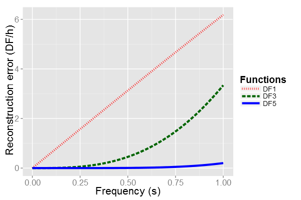
Table II shows the difference between the moments $m_{0},m_{1},m_{2},m_{3},m_{4}$ of $F^{0}_{q}$ and $F^{1}_{q}$ . We see that this difference is zero exactly for the first $q$ moments, $q=1,3,5$ . Figure 1 shows the difference $DF_{q}(s)={\cal F}(F^{0}_{q})(s)-{\cal F}(F^{1}_{q})(s)$ , for the frequency $s\in[0,1]$ . The normalized difference presented on the ordinate is $\frac{DF}{h}$ . In this figure we fix $\eta=0.05,h=0.1$ .

TABLE I: Signals parameters

	$a_{1}$	$a_{2}$	$a_{3}$	$x_{1}$	$x_{2}$	$x_{3}$
$F^{0}_{1}$	1	1	1	$-h-\eta$	$-\eta$	$+h+\eta$
$F^{1}_{1}$	1	1	1	$-h-\eta$	$+\eta$	$+h+\eta$
$F^{0}_{3}$	1	1	1	$-h-\eta$	$-\eta$	$+h+2\eta$
$F^{1}_{3}$	1	1	1	$-h-2\eta$	$+\eta$	$+h+\eta$
$F^{0}_{5}$	$-1-3\tilde{\eta}$	$2+3\tilde{\eta}$	$-1$	$-h-\eta$	$-\eta$	$h+2\eta$
$F^{1}_{5}$	$-1$	$2+3\tilde{\eta}$	$-1-3\tilde{\eta}$	$-h-2\eta$	$+\eta$	$+h+\eta$

TABLE II: Moments differences

	$\Delta m_{0}$	$\Delta m_{1}$	$\Delta m_{2}$	$\Delta m_{3}$	$\Delta m_{4}$
$F_{1}$	0	$2\eta$	0	$2\eta^{3}$	0
$F_{3}$	0	0	0	$6h^{2}\eta+18h\eta^{2}+16\eta^{3}$	0
$F_{5}$	0	0	0	0	0

Refer to caption — Fig. 1: Fourier differences $DF$ of the signals from Table I.

Acknowledgment

This research was supported by the ISF Grant No. 779/13.

References

[1] J.-M. Azaïs, Y. de Castro, and F. Gamboa, “Spike detection from inaccurate samplings,” Applied and Computational Harmonic Analysis, in press. [Online]. Available: http://www.sciencedirect.com/science/article/pii/S106352031400044X
[2] D. Batenkov, N. Sarig, and Y. Yomdin, “Accuracy of algebraic Fourier reconstruction for shifts of several signals,” Sampling Theory in Signal and Image Processing, vol. 13, no. 2, pp. 151–173, 2014.
[3] D. Batenkov and Y. Yomdin, “Algebraic signal sampling, Gibbs phenomenon and Prony-type systems.” in Proceedings of the 10th International Conference on Sampling Theory and Applications (SAMPTA), 2013.
[4] ——, “On the accuracy of solving confluent Prony systems,” SIAM J.Appl.Math., vol. 73, no. 1, pp. 134–154, 2013.
[5] ——, “Geometry and Singularities of the Prony mapping,” Journal of Singularities, vol. 10, pp. 1–25, 2014.
[6] D. Batenkov, “Accurate solution of near-colliding Prony systems via decimation and homotopy continuation,” arXiv:1501.00160 [cs, math], Dec. 2014, arXiv: 1501.00160. [Online]. Available: http://arxiv.org/abs/1501.00160
[7] ——, “Numerical stability bounds for algebraic systems of Prony type and their accurate solution by decimation,” arXiv preprint arXiv:1409.3137, 2014. [Online]. Available: http://arxiv.org/abs/1409.3137
[8] E. J. Candès and C. Fernandez-Granda, “Super-Resolution from Noisy Data,” Journal of Fourier Analysis and Applications, vol. 19, no. 6, pp. 1229–1254, Dec. 2013. [Online]. Available: http://link.springer.com/article/10.1007/s00041-013-9292-3
[9] ——, “Towards a Mathematical Theory of Super-resolution,” Communications on Pure and Applied Mathematics, vol. 67, no. 6, pp. 906–956, Jun. 2014. [Online]. Available: http://onlinelibrary.wiley.com/doi/10.1002/cpa.21455/abstract
[10] L. Demanet and N. Nguyen, “The recoverability limit for superresolution via sparsity,” Preprint, 2014.
[11] L. Demanet, D. Needell, and N. Nguyen, “Super-resolution via superset selection and pruning,” in Proceedings of the 10th International Conference on Sampling Theory and Applications (SAMPTA), 2013.
[12] D. L. Donoho and P. B. Stark, “Uncertainty principles and signal recovery,” SIAM J. Appl.Math., vol. 49, pp. 906–931, 1989.
[13] D. Donoho, “Superresolution via sparsity constraints,” SIAM Journal on Mathematical Analysis, vol. 23, no. 5, pp. 1309–1331, 1992.
[14] V. Duval and G. Peyré, “Exact support recovery for sparse spikes deconvolution,” arXiv preprint arXiv:1306.6909, 2013. [Online]. Available: http://arxiv.org/abs/1306.6909
[15] C. Fernandez-Granda, “Support detection in super-resolution,” in Proc. of 10th Sampling Theory and Applications (SAMPTA), 2013, pp. 145–148. [Online]. Available: http://arxiv.org/abs/1302.3921
[16] R. Heckel, V. I. Morgenshtern, and M. Soltanolkotabi, “Super-Resolution Radar,” arXiv:1411.6272 [cs, math], Nov. 2014, arXiv: 1411.6272. [Online]. Available: http://arxiv.org/abs/1411.6272
[17] S. Levy and P. K. Fullagar, “Reconstruction of a sparse spike train from a portion of its spectrum and application to high-resolution deconvolution,” Geophysics, vol. 46, no. 9, pp. 1235–1243, 1981.
[18] W. Liao and A. Fannjiang, “MUSIC for Single-Snapshot Spectral Estimation: Stability and Super-resolution,” arXiv:1404.1484 [cs, math], Apr. 2014. [Online]. Available: http://arxiv.org/abs/1404.1484
[19] C. W. McCutchen, “Superresolution in microscopy and the Abbe resolution limit,” J. Opt. Soc. Am., vol. 57, no. 10, pp. 1190–1190, 1967.
[20] K. Minami, S. Kawata, and S. Minami, “Superresolution of Fourier Transform spectra by autoregressive model fitting with singular value decomposition,” Appl. Optics, vol. 24, pp. 162–167, 1985.
[21] A. Moitra, “The Threshold for Super-resolution via Extremal Functions,” arXiv:1408.1681 [cs, math, stat], Aug. 2014, arXiv: 1408.1681. [Online]. Available: http://arxiv.org/abs/1408.1681
[22] V. I. Morgenshtern and E. J. Candes, “Stable super-resolution of positive sources: the discrete setup,” Preprint, 2014.
[23] J. Odendaal, E. Barnard, and C. W. I. Pistorius, “Two-dimensional superresolution radar imaging using the MUSIC algorithm,” IEEE Transactions on Antennas and Propagation, vol. 42, no. 10, pp. 1386–1391, 1994.
[24] D. Slepian, “Prolate spheroidal wave functions,” Fourier Analysis and uncertainty, V. - The discrete case. Bell System Technical Journal, vol. 57, pp. 1371–1430, 1978.
[25] Y. Yomdin, “Some quantitative results in singularity theory,” Ann. Polon. Math., vol. 87, pp. 277––299, 2005.
[26] ——, “Singularities in algebraic data acquisition,” Real and complex singularities, London Math. Soc. Lecture Note Ser., vol. 380, pp. 378–396, 2010.