Tensor decomposition with generalized lasso penalties
Abstract
We present an approach for penalized tensor decomposition (PTD) that estimates smoothly varying latent factors in multi-way data. This generalizes existing work on sparse tensor decomposition and penalized matrix decompositions, in a manner parallel to the generalized lasso for regression and smoothing problems. Our approach presents many nontrivial challenges at the intersection of modeling and computation, which are studied in detail. An efficient coordinate-wise optimization algorithm for (PTD) is presented, and its convergence properties are characterized. The method is applied both to simulated data and real data on flu hospitalizations in Texas. These results show that our penalized tensor decomposition can offer major improvements on existing methods for analyzing multi-way data that exhibit smooth spatial or temporal features.
Key words: multiway data, tensors, trend filtering, penalized methods, convex optimization
1 Introduction
1.1 Structure and sparsity in multiway arrays
In recent years there has been an increasing interest in the use of penalized methods for matrix and tensor decompositions. As in classical principal-components analysis (PCA), the goal of these methods is to represent a high-dimensional data matrix or multiway array in terms of a lower-dimensional set of latent factors. This line of work differs from classical techniques, however, in the use of penalty functions that encourage these estimated factors to be sparse, structured, or both. As many previous authors have demonstrated, such regularized estimators usually exhibit a favorable bias-variance tradeoff, particularly when the size of the array far exceeds the number of samples. They can also make the estimated factors themselves much more interpretable to practitioners.
Existing methods for penalized matrix decompositions have been shown to outperform classical PCA in discovering patterns in application areas such as genomics and neuroscience. Penalties that encourage structure (such as the fused lasso) provide interpretable results when there is a natural order of the measurements, while penalties that encourage sparsity are useful when there is no such ordering (Witten et al., 2009). In the high-dimensional tensor setting however, existing decomposition methods only enforce sparse constraints. We address this gap by proposing a method for penalized tensor decomposition (PTD) that allows arbitrary combinations of sparse or structured penalties along different margins of a data array.
Given a data array , the statistical problem that we study is to find a low-dimensional factor representation (also known as a Parafac decomposition) such that the factors are constrained to be sparse and/or smooth. For ease of presentation, we restrict attention to the three-way case, but the generalization of our approach to arrays with more than three modes is straightforward.
More explicitly, suppose we are given a set of observations , the elements of a three dimensional tensor , that have been generated from the complete tensor model
| (1) |
with unknown hidden vectors , and scalars . We will later discuss the missing data problem. For simplicity we assume that the variance of the error term is known and equal to . Moreover, when we suppress the index . Our goal is to estimate these latent factors, which can be challenging since we only have one observation for each combination . However, we assume that this task is aided by the presence of special structure in these true vectors. Explicitly, we assume that some of the vectors , are restrictions of smooth functions defined in the interval . For instance, it might be the case that for , where is a piecewise continuous or differentiable function on .
A natural situation in which this would arise is when one of the modes of the data array corresponds to a temporal or spatial axis. Our main contribution is to provide optimization algorithms for finding Parafac decompositions that shrink towards such structure. To do so, we apply a generalized lasso penalty along each mode of the array. We refer to this class of methods as penalized tensor decompositions (PTD).
We face two main challenges in estimating the factors. First, the resulting optimization problem is non-convex. We propose to reach a stationary point using block coordinate descent, as in Allen (2012), and we provide convergence rates for a single-block udpate. This leads us to the second challenge: unlike in the sparse unconstrained problem formulated by Allen (2012), for our case of a generalized lasso penalty, it is not clear how to make the block-coordinate updates. Our results provide a novel way of doing so that exploits the multi-convex structure of the problem, and that provides efficient algorithms for finding the factors when formulating the problem either in a penalized or constrained form.
1.2 Relation to previous work
Structurally constrained estimation is an active area of research, and we do not attempt a comprehensive review. Our work draws heavily in the one dimensional case on advances in understanding the one dimensional case, where penalized regression has been widely studied in the literature (Friedman et al., 2010; Kim et al., 2009; Tibshirani, 1996; Tibshirani et al., 2005). For instance, in protein mass spectroscopy and gene expression data measured from a microarray, the fused lasso has been used to obtain interpretable results (Tibshirani et al., 2005). The fused lasso is a natural choice here, since it encourages neighboring measurements to share the same underlying parameter. Similarly, to enforce smoothness in the solution, trend filtering has been proposed Kim et al. (2009) as a way to place one-dimensional function estimation within the convex optimization framework. The trend filtering penalized-regression problem has found applications in areas as diverse as image processing and demography.
In the case of matrix decomposition, the need for penalized methods arises in applications in genetic data, where there are multiple comparative genomic hybridizations and we expect correlation among observations at genetic loci that are close to each other along the chromosome. As shown in Witten et al. (2009), by considering different choices of penalties, we can recover different kinds of structures along either the rows or the columns of a data matrix. See the references in Witten et al. (2009) for a much more comprehensive bibliography on sparse principal components analysis.
In moving from matrices to multiway arrays, Parafac decompositions offer an attractive framework for recovering latent lower dimensional structure. This is due to their easy interpretability as well as feasibility of computation (Anandkumar et al., 2014; Harshman, 1970; Karatzoglou et al., 2010; Kolda and Bader, 2009; Kroonenberg, 2008). More generally, Tucker models have been proposed as general models for multiway data and have been successfully applied in many areas (Cichocki, 2013). Other popular methods for tensor decompositions include those described in Bhaskara et al. (2014) and De Lathauwer et al. (2000). However, these approaches do not provide structural or sparse solutions. This point was made by Allen (2012), who proposed a sparse penalized Parafac decomposition method that outperforms the classical Parafac decomposition when the true solutions are sparse. More recently, Sun et al. (2015) also considers sparse tensor recovery and provides statistical guarantees for such a task.
In this paper, we study methods for structured, as opposed to sparse, tensor factorizations. Our approach is inspired by the penalized matrix decomposition methods from Witten et al. (2009). We generalize the matrix-decomposition problem to the framework of tensor Parafac decompositions while incorporating solution algorithms for a more broad class of penalties, including trend filtering for factors that are smooth (e.g in space or time).
1.3 Basic definitions
We now introduce notation and definitions used throughout the paper. This material can be found in Cichocki et al. (2009), to which we refer the reader for more details. Let …, denote index upper bounds. A tensor of order is an way array where elements are indexed by for = Tensors are denoted by capital letters with a bar, e.g. . Matrices are denoted by capital letters, e.g , and for a matrix we denote by its generalized inverse. Vectors are denoted by lower case letters, e.g . The outer product of two vectors and yields a rank-one matrix , and the outer product of three vectors and yields a third-order rank-one tensor. We use to indicate the usual Frobenius norm of tensors. The mode- multiplication of a tensor by a vector is denoted by , and element-wise we have .
1.4 Outline
The rest of the paper is organized as follows. Section 2 defines our statistical approach to rank-1 tensor decompositions based on generalized lasso penalties. Section 3.1 then provides solution algorithms for our problem formulation when the penalties are used to define a set of constraints on the parameters. This is done by exploiting the efficiency of solution-path algorithms for generalized-lasso regression problems. In Section 3.2, we then study an unconstrained version of the problem where the penalties enter directly into the objective. Because the original problem is not convex, this is not equivalent to the constrained formulation, and some important algorithmic differences are highlighted. After developing algorithms for rank-1 tensor decompositions, Section 3 concludes by extending these ideas to the general case of multiple factors.
Section 4 presents a convergence analysis for our fundamental rank-1 decomposition algorithm. In Section 5, using simulated data, we benchmark against state-of-the-art methods on rank-1 and multiple factor decompositions, measuring the error of recovery with the Frobenius norm. We then validate our algorithms on two real data sets involving flu hospitalizations in Texas and motion-capture data. Finally, Section 6 present a brief discussion of the overall framework proposed in this paper.
2 Penalized tensor decompositions
We first consider the case . Taking a point of view similar to Witten et al. (2009), for positive constants , and , we formulate the following problem:
| (2) | ||||||
where , and are matrices which are designed to enforce structural constraints. When the context is clear we will suppress the superscript and simply use the notation . We note that an alternative, although non-equivalent, formulation is based on an unconstrained version of (2) given as
| (3) |
with the same unit-norm constraints on the factors. In Section 3, we will discuss the computational differences between these formulations in detail.
We now briefly discuss a broad class of penalties of potential interest to practitioners. We focus on choices that penalize first- and higher-order differences in each factor, which correspond to the fused lasso and trend filtering, respectively (Tibshirani, 2011). The fused lasso penalty was suggested in Witten et al. (2009) to detect regions of gain for sets of genes in matrix-decomposition problems. For this penalty, the associated matrix is the first-difference matrix, if , if and otherwise. As discussed in Tibshirani (2011), this penalty gives a piecewise-constant solution to linear-regression problems, and it is used in settings where the coordinates in the true model are closely related to their neighbors. A related choice for is oriented incidence matrices of a graph; see, e.g. Arnold and Tibshirani (2015). These are constructed as generalizations of the 1-dimensional fused lasso on an underlying graph .
Still other choices for correspond to polynomial trend filtering, which impose a piecewise polynomial structure on the underlying object of interest. These are constructed as follows. First define the polynomial trend filtering of order as where and is the first order difference matrix. Then, recursively construct the polynomial trend filtering matrix of order as .
The polynomial trend filtering fits (especially for ) are similar to those that one could obtain using regression splines and smoothing splines, However, the knots (changes in kth derivative) in trend filtering are selected adaptively based on the data, jointly with the inter-knot polynomial estimation (Tibshirani, 2011). A comprehensive study of polynomial trend filtering can be found in Tibshirani et al. (2014). We note that Problem (3) was already studied in Allen (2012) for the case in which all the matrices , and are set to be the identity. This is the case of having the L1 penalty on each mode. The authors in Allen (2012) proposed a fast algorithm to solve the problem. However, the L1 penalty has the disadvantage of encouraging only sparsity. If the true factors are not sparse but instead locally flat or smooth, then having sparse constraints on the factors performs poorly. This phenomenon was observed in Witten et al. (2009) in the context of matrix decompositions, where the fused lasso penalty was shown to properly recover flat vectors in the factors of the decomposition when the L1 penalty failed to do so. We will extend these ideas to tensor decompositions, applying penalties from the generalized lasso class. We now turn to the question of how to fit these models efficiently.
3 Solution algorithms
3.1 Constrained problem
Since (2) is a non-convex problem, we propose to consider a block coordinate-descent routine. However, in order to have convex block-coordinates-updates, we instead state the following problem:
| (4) | ||||||
This differs from (2) in two ways. First, the objective has been reformulated in a more convenient way, but it is easy to show that this results in an equivalent problem (Kolda and Bader, 2009). Secondly, the unit norm constraints have been relaxed to the convex constraints that each factor fall into the unit ball. Additionally, following Witten et al. (2009), a simple modification can naturally handle missing data. Denoting by the set missing observations, we solve the missing data problem by replacing the objective function in (4) with the function
| (5) |
Note that (4) has a multilinear objective function in , , and . Since the penalties induced by , and are convex, we can use coordinate-wise optimization in order to solve this problem. For example, when and are fixed, the update for is found by solving the following problem:
| (6) |
It would seem that a solution to (6) would not in general have unit norm. But it is possible to ensure that this will be the case—that is, to ensure the solution follows on the boundary of the constraint set—as long as is chosen properly based on the KKT conditions. A similar phenomenon was observed for the matrix case in Witten et al. (2009). One of our results is that the solution to (6) will very often turn out to have unit norm, despite our convex relaxation. A rigorous statement of this result will be given later.
Our strategy to solve (4) is to sweep through the vectors iteratively by proceeding with block coordinates updates. Thus starting from initials , and , we proceed by solving, at iteration , the problems shown in Algorithm 1. It should be pointed out here that the best we can hope with Algorithm 1 is to obtain a local minimum to (4). It will be shown latter with our experiments that this local minimum provides interpretable and accurate estimators. Note that while the algorithm is structurally quite simple, the individual block-coordinate updates are non-trivial to solve efficiently. The remainder of this section discusses how this can be done.
Given the symmetry of the problem, without loss of generality, we focus on the update for . We notice that the constraint set involves a non-differentiable function, implying that it is not possible to use a gradient-based method. Before describing our approach, we first discuss two natural possibilities and explain why they were ultimately rejected.
First, a simple approach is to include a slack variable and use the ADMM algorithm. However, the resulting update for would require solving a constrained problem using, for example, an interior-point method. This rapidly becomes infeasible, since it requires solving a large dense linear system.
A second natural approach is to use the novel ADMM algorithm from Zhu (2015) to solve each of the block-coordinate updates. For instance, the update for would involve solving the problem
| (7) |
where is a matrix such that . Then proceeding as in Zhu (2015), we observe that (17) can be solved in linear time, as the update for is a simple projection on the unit ball, while the update for requires projecting in a ball with the algorithm from Duchi et al. (2008). (The actual updates for our problem are given in the appendix.) However, while this algorithm indeed solves the constrained-problem updates, we find in that practice the ADMM routine requires a long time to converge. In particular, it presents problems enforcing the constraint that , so that the solution returned after reasonable runtimes is actually quite far from the feasible region.
This motivates us to consider a different approach to solve the block-coordinate updates in (1). We appeal to the following theorem, which suggests a simple method and also implies that, typically, the solution lies on the boundary of the unit ball. That is, it satisfies the non-convex constraint of problem (2), despite our relaxation.
Theorem 1.
As a direct consequence of the proof of Theorem 1, we can solve (6) by first solving (9) with the solution-path algorithm from Tibshirani (2011), then finding and finally . The explicit algorithm is given in the appendix.
Unfortunately, there is no characterization available of of the computational time to compute the solution path. It is only known the cost at each iteration is in its worst case, but it is unknown how many kinks that a particular problem will have. Moreover, we notice that after the solution path is computed, the next two steps require cost. Therefore, the total cost for updating is .
3.2 Unconstrained version
The framework we have introduced for rank-1 approximations has some nice features. In particular, the choice of tuning parameters is more intuitive, since this directly imposes a constraint on the smoothness of the solutions. However, the optimization routine derived from Theorem 1 is computationally intensive. In particular, for large dimensions of the penalty matrices, computing the entire solution path can still be somewhat slow. To avoid this, we revisit (3) and consider a problem equivalent to its convex relaxation:
| (11) | ||||||
As in the constrained case, we solve (11) via block-coordinate updates. Now the update for is obtained by solving
| (12) |
The solution to (12) can be characterized in the same manner as for the constrained case. In fact, the proof of Theorem 1 implies the following corollary:
Corollary 2.
An interesting consequence of the closed-form formula (14), and the proof of Theorem 1, is that we can solve (12) by first solving a generalized lasso problem and then projecting the solution into the unit ball. Explicitly, we first find
| (15) |
and becomes the solution to (12). Therefore, for trend-filtering problems, we can solve the regression problem step with the fast ADMM algorithm from Ramdas and Tibshirani (2015). Moreover, for the case of a fused lasso penalty, the update for can be done in linear time (Johnson, 2013). Because these two algorithms are so efficient, the penalized formulation from (11) can be solved much more cheaply than the constrained formulation from (4).
3.3 A toy example
We illustrate the advantage of problem (11) over the formulation from (4) using a toy example. We consider and as the size of varies. Here, and are as in Structure 2 in Figure 2, while is the function evaluated at evenly spaced locations in . Taking initial values from the power method, we compare the solutions from one iteration of the unconstrained formulation when choosing the penalty parameters adaptively, versus an “oracle” version of the constrained problem with . This choice of hyperparameters for the constrained problem is obviously optimal, but requires knowledge of the true factors, and is therefore unrealistic in practice.
Figure 1 demonstrates the favorable trade-off offered by the unconstrained formulation with adaptively chosen tuning parameters. We observe that while the constrained formulation algorithm based on the solution-path computation is the most accurate, the unconstrained formulation is competitive in terms of reconstruction error, and much more efficient. The ADMM algorithm based on Zhu (2015) is substantially less accurate than the other two methods.
Moreover, in practice it would be necessary to solve the constrained problem with more than one value of the tuning parameters, since we do not know . Hence the penalized version is strongly preferred: we can do adaptive parameter choice more cheaply than solving the constrained version for a single hyperparameter setting, without a major loss of performance even under an optimal hyperparameter choice.


With regards to the choice of regularization, we can consider two alternatives based on cross validation. The first of these follows Witten et al. (2009). This procedure involves randomly deleting a percentage of the input data and solves the problem on the resulting tensor. The estimated tensor produces predicted values on the deleted entries, allowing one to compute mean square error of prediction for these notionally missing values. The parameters , and are then chosen to minimize the prediction error. This is particularly attractive when multiple processors are available, given that independent problems with different tuning parameters can be solved in parallel.
The other alternative for cross validation applies to (11) and it is based on adaptively choosing the tuning parameters. Thus, before estimating each vector (say ), we obtain a generalized lasso regression problem and hence we can choose by cross validation. We randomly separate the coordinates of the response vector into training and test set, solving the problem in the training set and computing the mean squared error of the predicted solution on the test set. This exploits the fact that is a smooth function, and therefore given a solution based on the training set, we can provide estimates at the locations in the test set by interpolation.
3.4 Multiple factors
In the case of multiple factors, the main difference of the tensor case versus the matrix case is that we must find all the factors jointly (Kolda and Bader, 2009), as opposed to estimating factor using the residual from the fitted -factor model. Fortunately, it is straightforward to use any of the algorithms in the previous section to handle multiple factors. Hence, to estimate the factors in (1), we state the problem
| (16) | ||||||
where the matrices , and are chosen to capture different structural features desired for the solutions. Here, , and are tuning parameters. Now we solve (16) by starting with initial guesses , , , and applying the iterative updates listed in Algorithm 2 exploiting results from Section 3.2.
In practice the number of latent factors can be chosen with an ad-hoc rule by looking at the proportion of the variance explained (as with a scree plot in ordinary PCA). One can look at the solutions provided by different values of . The choice of then corresponds to the number factors such that the increase in variance explained obtained by solving the problem with more factors is negligible. We illustrate this in our real data example.
Finally, in situations where the number of factors is large, the number of possible combinations of tuning parameters becomes challenging. One possibility to address this is to choose the parameters adaptively as discussed in Section 3.2. Hence, every time a factor is to be updated we select the parameter from a small grid of values. This ensures that, for instance, when dealing with fused lasso penalties each block coordinated update can be done in linear time. On the other hand, a different alternative is to use the same penalty parameter for all the vectors corresponding to the same level of smoothness. For instance, one can use if . This reduces the burden of cross-validation.
4 Convergence analysis
We now examine the convergence of the block-coordinate algorithms developed in the previous section. Here, we assume that in Model (1). In this case we recall that the underlying true tensor can be decomposed as the outer product of vectors and times a constant . Moreover, we assume that the matrices are chosen to be either fused lasso or trend filtering penalties. Thus, , and with and .
Our proof is inspired by the work on convergence rates for generalized lasso regression problems from Wang et al. (2014). The theorem states that, when starting with good initials, it is necessary to sweep through the data only once. The proof of the claim is based on the identity
for any events , and . A related statement can be made in the case of multiple factors for a single update depending on the other factors. See the result in the appendix; the main difference there involves an error measurement that depends on the factors taken as fixed.
Theorem 3.
Let denote a one-step update from Algorithm 1, based on initial values , and assume that , , and . Then, there exists a constant such that if satisfies
and
then
where
Theorem 3 states that with good initials our rank-1 decomposition algorithm will be very close to the true factors under weak assumptions concerning the smoothness of the true factors. Thus, in practice before running our algorithms, we can consider a simple initialization that consists od solving Algorithm (1) for the case where the matrices , and are all zero. This is known as the power method (Kolda and Bader, 2009). Moreover, statistical guarantees for a very related method to this procedure were studied in Anandkumar et al. (2014).
Finally, it should be note that Theorem 3 implicitly suggests that an appropriate choice of tuning parameter is which only involves the true latent vectors. In the case of the unconstrained version, a very similar statement to Theorem 3 holds by taking , and .
Finally, we note that, as one would expect, the larger is, the better we should expect to perform. This is intuitive, given that when increases and the unit vectors , and are fixed, the standard Gaussian noise becomes small compared to the magnitude of the observations.

5 Experiments
Our experiments focus mainly on the task of rank-1 recovery, since all of our algorithms are based on the development of a rank-1 PTD. For all our simulations we use the Frobenius norm of the difference between the estimated and true tensors as a measure of overall accuracy. The Frobenius norm is a natural choice of model fit, since we also benchmark against a recovery method that does not directly produce a rank-1 tensor but does provide an estimate of the true mean tensor. This method is based on the idea of stacking several penalized matrix decompositions using the technique from Witten et al. (2009). Specifically, we consider the tensor of observations as a collection of 10 distinct matrices, each of which is estimated via a rank-1 PMD. This will lead to 10 estimated rank-1 matrices which are concatenated to build a 10 1000 400 tensor. We call this procedure, with an abuse of notation, PMD where and are the penalties on and , when computing the rank-1 PMD matrices.
The other methods included in the study are the PTD with different penalties denoted as PTD. We consider choices such as the L1 penalty, the fussed lasso (FL) and trend filtering of order k (TFk). Note that we are implicitly comparing to the method from Anandkumar et al. (2014) since, for rank-1 recovery, this reduces to the power method, and hence to PTD(L1,L1,L1) for appropriate parameters.
For our simulations, the tuning parameters by cross validation on a grid of possible values for each of the parameters , , and . In every experiment, we randomly select of the data for testing, using the other as training data. Out of a range of candidate tuning parameters we select those that produce the smallest error on the 10 held-out set. This process is repeated for each of 100 simulations, for different methods and structures, in order to obtain average Frobenius errors for all the competing methodologies with respect to every structure.
To see how different choices of penalties can behave under different scenarios, we ran experiments using five different rank-1 tensors as the true mean tensor. These choices are designed to explore a range of plausible structures that we might find in real problems. For the first structure both and are piecewise flat. For the second, both and are periodic functions. For the third, both and are piecewise quadratic polynomials. For the fourth, is smooth and is piecewise constant. For the fifth, both and are sparse but with no specific structural pattern like smoothness or flatness. The goal of this final scenario is to understand how structural penalties perform in a data set where they are not warranted. Further details of this simulation are included in the appendix. Figure 2 also shows a plot of these different structures.
| Method | Structure 1 | Structure 2 | Structure 3 | Structure 4 | Structure 5 |
|---|---|---|---|---|---|
| PTD(L1,L1,L1) | 37.37 | 47.63 | 46.16 | 39.91 | 40.58 |
| PTD(L1,FL,FL) | 6.31 | 27.54 | 11.76 | 10.30 | 57.15 |
| PTD(L1,TF1,FL) | 15.07 | 20.49 | 11.55 | 9.00 | 70.32 |
| PTD(L1,TF1,TF1) | 17.61 | 14.40 | 11.85 | 12.40 | 79.25 |
| PMD(L1,L1) | 85.05 | 89.10 | 100.70 | 91.89 | 72.87 |
| PMD(L1,FL) | 49.09 | 50.14 | 52.70 | 22.73 | 92.20 |
| PMD(FL,FL) | 15.05 | 43.17 | 25.64 | 33.95 | 114.09 |
The results of our simulation study are shown in Table 1. In all cases, PTD converged with few iterations, usually less than 10. From these results, it is clear that different choices of penalty are suitable for different problems. For structure 1, in which the true and are piecewise flat, the combination PTD(L1, FL, FL) outperforms all the other choices that we considered. Interestingly, PTD(L1,TF1,FL) and PTD(L1, TF1,TF1) provided better results than the “stacking” method PMD(FL,FL). Note also that PTD(L1,TF1,FL) and PTD(L1,TF1,TF1) behave fairly similar to one another. This is reasonable since a piecewise constant function is a special case of a piecewise linear function and hence we would expect that TF1 would produce only slightly worse results than fused lasso.
| Method | |||||
|---|---|---|---|---|---|
| PTD(L1,L1,L1) | 62.66 | 81.66 | 80.46 | 99.50 | 94.37 |
| PTD(L1,FL,FL) | 32.61 | 38.80 | 41.63 | 46.32 | 49.33 |
| PTD(L1,TF1,FL) | 24.55 | 28.55 | 32.35 | 37.87 | 38.43 |
| PTD(L1,TF1,TF1) | 17.00 | 21.35 | 22.27 | 27.09 | 27.36 |
| PMD(L1,L1) | 116.19 | 139.57 | 158.71 | 185.05 | 209.45 |
| PMD(L1,FL) | 66.80 | 76.81 | 83.65 | 98.18 | 111.09 |
| PMD(FL,FL) | 52.43 | 57.52 | 65.36 | 83.98 | 92.71 |
Moreover, Table 1 also illustrates when our methodology should not be expected to work. This is what happens with structure 5, where there is no spatial pattern in the true vectors , and , and instead they are merely sparse (80 of their coordinates are zero). Here, as expected, PTD(L1,L1,L1) outperforms any of our methods.
In the previous experiment we simulated all data sets with the assumption that the noise had variance 1. Now we fix the rank-1 tensor mean of Structure 2, where both and are periodic functions, and then we compare the performance of different methods as the standard deviation of the noise changes. Recalling that in Structure 2 both and are periodic smooth, it does not come as a surprise that PTD(L1,TF1,TF1) provides the best performance in all situations considered in Table 2. In addition, it is clear that the error of all methods increases as the variance of the noise does. Nevertheless, the performance of our method seems to tbe the most stable.
| Method | Structures | |||||||||
|---|---|---|---|---|---|---|---|---|---|---|
| 1,2 | 1,3 | 1,4 | 2,3 | 2,4 | 3,4 | 1,2,3 | 1,2,4 | 1,3,4 | 2,3,4 | |
| Anandkumar | 544.0 | 310.5 | 85.4 | 121.0 | 128.9 | 273.4 | 534.9 | 555.3 | 346.6 | 350.3 |
| PTD(L1,FL,FL) | 55.3 | 46.5 | 27.1 | 71.2 | 59.7 | 107.3 | 184.2 | 48.3 | 102.8 | 126.1 |
| PTD(L1,TF1,TF1) | 51.7 | 71.6 | 67.8 | 49.2 | 50.9 | 94.0 | 120.3 | 75.2 | 141.6 | 120.8 |
Finally, we evaluate the recovery of mean tensors having multiple factors, with . Scenarios where the true model consists of and are considered. Our comparisons are based on taking sums of different rank-1 tensors using the structures discussed before. The competing methods are PTD(L1,FL,FL) and PTD(L1,TF1,TF1), versus Algorithm 1 from Anandkumar et al. (2014). For the latter, we set the number of initializations and the number of iterations . The results in Table 3 show a clear gain for our approach over the method from Anandkumar et al. (2014), which do not impose any smoothness constraints on its solutions.
6 Real data examples
6.1 Flu hospitalizations in Texas
As a simple illustrative example, we consider measurements of flu activity and atmospheric conditions in Texas, see the appendix for information how to collect the data. There are 5 variables measured daily across 25 cities in Texas from January 1, 2003 to December 31, 2009. The variables are: maximum and daily average observed concentration of particulate matter (air quality measure), maximum and minimum temperature, and a measure of flu intensity capturing flu-related hospitalizations per million people. The data tensor is thus a 5x25x2556 array where we expect clear temporal patterns, along with correlations among the five variables. For example, during the winter months we would expect an increase in flu-related hospitalizations, correlated with seasonal patterns of maximum and minimum daily temperatures.
To show the kind of interesting results that one can get with our methods, we compute a two-factor Parafac decomposition. We use trend filtering of order 2 in the temporal mode and no penalty on the other two modes (although it would be straightforward to incorporate a penalty on the spatial mode as well.) We use our main result (1) to find the factors using coordinate-wise optimization. The tuning parameter for the trend-filtering penalty is chosen by cross validation from a grid of values to ensure that we get a smooth vector for the time mode.
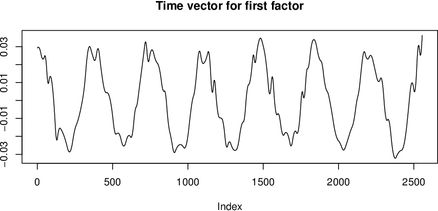


We considered fitting models with different values of , we found that a model with one factor explains of the variance, a model with two factors explains percent of the variance, and a model with three factors results in increase in variance explained of less than with respect to the case . Moreover, the model with 3 factors results in highly correlated factors. For this reason we use a model with factors.
From Figure 3 we note a clear seasonal effect. In the first factor we observed that the loadings for the flu intensity, minimum temperature, and maximum temperature can be all explained in a similar way. For the first of these three variable the loadings are positive in every city. Hence, given the shape of the time vector we see a periodic pattern of flu cases across cities with the highest during the winter months and the lowest during the summer months.
6.2 Motion capture data
For a more challenging task, we evaluate the performance of our PTD method using data from the motion capture (moCap) repository at mocap.cs.cmu.edu. This consists of subjects performing different physical activities in repeated independent trials. We construct 3-array tensors by taking sets of videos as one mode, 12 representative variables of the body movements as the second mode, and data frames in time as the third mode. The 12 variables are listed in the appendix.
We built 2 tensors each for 5 different tasks, with each task generating a training-set tensor and a test-set tensor. The training set tensor corresponds to a single subject performing multiple repetitions of a single related set of physical activities. Similarly, the corresponding test-set tensor corresponds to that same subject performing further repetitions of those same activities. For example, the first data set (comprising 1 tensor in the training set and 1 tensor in the test set) is called 126-swimming; this is formed by looking at 8 videos of subject 126 performing different swimming styles. In the moCap repository, videos 1,3,6,8 are used for training while videos 2,4,7,9 are used for testing. This results in both tensors having dimensions 425312.
The other four data sets, explained in detail in the appendix, are 138-story (subject 138 walking and moving arms); 107-walking (subject 107 walking with obstacles); 9-running (subject 9 running); and 138-marching (just like it sounds). For these data sets, the tensors dimensions are 432512, 482812, 412812, 437112 respectively.
In this context, our PTD approach can be thought of as a smoothing step applied to the training-set tensor, to yield better out-of-sample predictions for the test-set tensor. We evaluate the performance of the method by calculating the reconstruction error (again, by Frobenius norm) when using the fitted/smoothed training-set tensor to predict the corresponding test-set tensor.
We find that for the tensors considered here, rank-1 is the best Parafac decomposition, since models with higher factors result in strongly correlated factors. We ran our rank-1 PTD with a trend-filtering penalty of order 2 on the second mode, and no constraints in the other modes. We compare against the PMD using the same degree of smoothness, as well as the classical PCA method from Anandkumar et al. (2014). From Table 4 it is clear that PTD offers the best performance. Thus we can see the gain of using smooth penalties, reflecting the fact that physical movements involve motion-capture variables that change smoothly in time. Moreover, it is clearly favorable to pool information across videos, as our method does, rather than treating them independently, as with the PMD algorithm.
| Method | Task | ||||
|---|---|---|---|---|---|
| 126-swimming | 138-story | 107-walking | 9-running | 138-marching | |
| Anandkumar | 254.80 | 134.63 | 135.17 | 84.40 | 143.86 |
| PTD(L1,TF2,TF2) | 250.98 | 131.78 | 134.92 | 84.29 | 142.44 |
| PMD(L1,TF2,TF2) | 267.89 | 145.14 | 143.43 | 88.06 | 149.41 |
7 Discussion
In many problems, tensors offer a natural way to represent high-dimensional, multiway data sets. However, tensors by themselves are difficult to interpret, creating the need for methods that shrink towards some simpler, low-dimensional structure.
Parafac models have been widely used for this task, but existing state-of-the-art methods typically constrain the factors to be orthogonal, or simply do not enforce any constraints. As we have shown, this can be undesirable in practice, especially if one is looking for more interpretable factors, where there is a natural spatial or temporal relation between observation, and it is expected that the factors will be smooth. We fill this gap by providing a set of methods that precisely offer piecewise smooth Parafac decompositions. Our methods exploit state of the art convex optimization algorithms and are shown to have excellent performance in our experiments. We leave for future work the study of algorithms for more general classes of penalties that can potentially be non-convex.
Finally, we have shown two alternatives for finding our smooth tensor decompositions with generalized lasso penalties. The constrained formulation seems to be an attractive option for practitioners, with clear intuitive control over the level of smoothness exhibited by the solutions. On the other hand, in light of its computational advantages, the unconstrained formulation offers a more practical approach, especially if there is no pre-existing knowledge about the anticipated smoothness of the solutions.
References
- Allen (2012) G. Allen. “Sparse higher-order principal components analysis”. In International Conference on Artificial Intelligence and Statistics, pages 27–36, 2012.
- Anandkumar et al. (2014) A. Anandkumar, R. Ge, and M. Janzamin. “Guaranteed Non-Orthogonal Tensor Decomposition via Alternating Rank-1 Updates”. arXiv preprint arXiv:1402.5180, 2014.
- Arnold and Tibshirani (2015) T. Arnold and R. Tibshirani. “Efficient Implementations of the Generalized Lasso Dual Path Algorithm”. Journal of Computational and Graphical Statistics, (just-accepted), 2015.
- Banerjee et al. (2004) S. Banerjee, A. E. Gelfand, and B. P. Carlin. “Hierarchical modeling and analysis for spatial data”. Crc Press, 2004.
- Bhaskara et al. (2014) A. Bhaskara, M. Charikar, A. Moitra, and A. Vijayaraghavan. “Smoothed analysis of tensor decompositions”. pages 594–603, 2014.
- Boyd and Vandenberghe (2004) S. Boyd and L. Vandenberghe. “Convex optimization ”. Cambridge Univ. Pr, 2004.
- Cichocki (2013) A. Cichocki. “Tensor Decompositions: A New Concept in Brain Data Analysis?”. arXiv preprint arXiv:1305.0395, 2013.
- Cichocki et al. (2009) A. Cichocki, R. Zdunek, A. H. Phan, and S.-i. Amari. “Nonnegative matrix and tensor factorizations: applications to exploratory multi-way data analysis and blind source separation”. John Wiley & Sons, 2009.
- De Lathauwer et al. (2000) L. De Lathauwer, B. De Moor, and J. Vandewalle. “A multilinear singular value decomposition”. SIAM journal on Matrix Analysis and Applications, 21(4):1253–1278, 2000.
- Duchi et al. (2008) J. Duchi, S. Shalev-Shwartz, Y. Singer, and T. Chandra. Efficient projections onto the l 1-ball for learning in high dimensions. In Proceedings of the 25th international conference on Machine learning, pages 272–279. ACM, 2008.
- Friedman et al. (2010) J. Friedman, T. Hastie, and R. Tibshirani. “Applications of the lasso and grouped lasso to the estimation of sparse graphical models”. Technical report, Technical report, Stanford University, 2010.
- Harshman (1970) R. A. Harshman. “Foundations of the parafac procedure: models and conditions for an ”explanatory” multimodal factor analysis”. 1970.
- Hoff et al. (2011) P. D. Hoff et al. “Separable covariance arrays via the Tucker product, with applications to multivariate relational data”. Bayesian Analysis, 6(2):179–196, 2011.
- Johnson (2013) N. A. Johnson. “A Dynamic Programming Algorithm for the Fused Lasso and L 0-Segmentation”. Journal of Computational and Graphical Statistics, 22(2):246–260, 2013.
- Jolliffe et al. (2003) I. T. Jolliffe, N. T. Trendafilov, and M. Uddin. “A modified principal component technique based on the LASSO”. Journal of Computational and Graphical Statistics, 12(3):531–547, 2003.
- Karatzoglou et al. (2010) A. Karatzoglou, X. Amatriain, L. Baltrunas, and N. Oliver. “Multiverse recommendation: n-dimensional tensor factorization for context-aware collaborative filtering”. In Proceedings of the fourth ACM conference on Recommender systems, pages 79–86. ACM, 2010.
- Kim et al. (2009) S.-J. Kim, K. Koh, S. Boyd, and D. Gorinevsky. “ Trend Filtering”. Siam Review, 51(2):339–360, 2009.
- Kolda and Bader (2009) T. G. Kolda and B. W. Bader. “Tensor decompositions and applications”. SIAM review, 51(3):455–500, 2009.
- Kroonenberg (2008) P. M. Kroonenberg. “Applied multiway data analysis”, volume 702. John Wiley & Sons, 2008.
- Leng and Tang (2012) C. Leng and C. Y. Tang. “Sparse matrix graphical models”. Journal of the American Statistical Association, 107(499):1187–1200, 2012.
- Lu et al. (2008) H. Lu, K. N. Plataniotis, and A. N. Venetsanopoulos. “MPCA: Multilinear principal component analysis of tensor objects”. Neural Networks, IEEE Transactions on, 19(1):18–39, 2008.
- Ramdas and Tibshirani (2015) A. Ramdas and R. J. Tibshirani. “Fast and flexible admm algorithms for trend filtering”. Journal of Computational and Graphical Statistics, (just-accepted), 2015.
- Sun et al. (2015) W. Sun, J. Lu, H. Liu, and G. Cheng. “Provable Sparse Tensor Decomposition”. arXiv preprint arXiv:1502.01425, 2015.
- Tibshirani (1996) R. Tibshirani. “Regression shrinkage and selection via the lasso”. Journal of the Royal Statistical Society. Series B (Methodological), pages 267–288, 1996.
- Tibshirani et al. (2005) R. Tibshirani, M. Saunders, S. Rosset, J. Zhu, and K. Knight. “Sparsity and smoothness via the fused lasso”. Journal of the Royal Statistical Society: Series B (Statistical Methodology), 67(1):91–108, 2005.
- Tibshirani (2011) R. J. Tibshirani. “The solution path of the generalized lasso”. The Annals of Statistics, 39(3):1335–1371, 2011.
- Tibshirani et al. (2014) R. J. Tibshirani et al. “Adaptive piecewise polynomial estimation via trend filtering”. The Annals of Statistics, 42(1):285–323, 2014.
- Wang et al. (2014) Y.-X. Wang, J. Sharpnack, A. Smola, and R. J. Tibshirani. “Trend Filtering on Graphs”. Journal of Machine Learning Research, (To appear), 2014.
- Witten et al. (2009) D. M. Witten, R. Tibshirani, and T. Hastie. “A penalized matrix decomposition, with applications to sparse principal components and canonical correlation analysis”. Biostatistics, page kxp008, 2009.
- Zhao et al. (2013) Q. Zhao, C. F. Caiafa, D. P. Mandic, Z. C. Chao, Y. Nagasaka, N. Fujii, L. Zhang, and A. Cichocki. “Higher Order Partial Least Squares (HOPLS): A Generalized Multilinear Regression Method”. Pattern Analysis and Machine Intelligence, IEEE Transactions on, 35(7):1660–1673, 2013.
- Zhu (2015) Y. Zhu. An augmented admm algorithm with application to the generalized lasso problem. Journal of Computational and Graphical Statistics, (just-accepted), 2015.
Appendix A ADMM algorithm to solve the constrained updates
In this section we discuss how to find the updates for Algorithm 1 from the main document using the ADMM algorithm from Zhu (2015). Since these are symmetric we focus on the particular update . In this case the problem is
| (17) |
We define as
and solve (17), using the ADMM algorithm from Zhu (2015), by considering the iterative updates
where the update for can be done using the algorithm from Duchi et al. (2008).
As explained in the main manuscript, in practice, using update as part of an ADMM algorithm leads to difficulty enforcing the constraint in reasonable runtimes, and results in larger reconstruction error than the technique we have recommended.
Appendix B Proof of technical results
B.1 Proof of Theorem 1
Note that the Lagrange dual function of the original problem is given by
Next, define for fixed the function given by
| (18) |
From (18) we need to solve the following problem:
| (19) |
which can be rewriten as
This problem has the following Lagrangian:
which is nicely separable in and .
Let us now consider some special cases of and . First, if and , then clearly,
Second, if and , then
Next, if and , then
and
Thus
Finally, let us now focus on or Then
while (see Tibshirani (2011))
Hence, the dual problem to (19) is equivalent to
But for fixed, this is equivalent to solving the problem
| (20) |
which can be solved for every using the solution path algorithm from Tibshirani (2011).
Let us denote by the solution to (20) for a fixed Therefore,
which implies that the dual to the original problem becomes
| (21) |
Finally, recall from Boyd and Vandenberghe (2004) that any solution to the original problem must also solve
for and that are optimal for (21). However, the objective function in (19) is strictly convex since and so its solution is unique and also solves
The KKT optimality conditions for this problem imply that
for some subgradient of the function at Therefore
and the result follows.
B.2 Proof of Theorem 2
Here we assume that data is generated as
and
Under these conditions we show that defined as
satisfies
The proof will then follow by an application of this claim after each block update, and applying the identity for the intersection of such events (see the main paper).
To prove the claim above, we start by noticing that
Next we use the notation for the row space of : and . Moreover, denotes the perpendicular projection onto the space . Hence, by suboptimality,
| (22) |
Let us now bound the terms in the expression above. First, let be an orthonormal basis of . Then
| (23) |
for some constant with probability at least
Here we have used Mill’s inequality and the fact that we can take . The latter claim is immediate for . If it can be proven as follows. First, we set . Then by the definition of , an induction argument shows that
| (24) |
for , where is the th coordinate of . But since is a unit vector, simple algebra yields
| (25) |
Now, since and are orthogonal, we must have
Next we bound the term involving the projection operator onto the space in (22). By Holder’s inequality,
and hence, as in Corollary 4 from Wang et al. (2014), we find that
| (27) |
On the other hand, by the Cauchy–Schwarz inequality, we have
| (28) |
Combining (22), (23), (27), (28), and proceeding in similar fashion for the other updates, the identity
for any events , and implies the result.
For the case of multiple factors, we have the following result. Suppose that the data is generated as
where is tensor of white noise. Suppose that we have current parameters estimates of , , , which we denote by , , , .
Let us now provide an error bound for the estimate of given all the other estimates. To that end, define
and assume that and
This leads to the following lemma.
Lemma 4.
Under the definitions just given,
where
Proof.
To show this we proceed as follows. We start noticing that, by sub-optimality,
and hence the claim follows for the case .
∎
Appendix C Discussion and extensions
C.1 Further connections with existing work
In recent years, many different efforts have been made to apply the ideas of sparse regression and sparse matrix decomposition to the context of higher-order tensors. Our paper has shown that structured penalties from the generalized-lasso class can offer significant modeling benefits when the underlying factors are piecewise constant or smooth. Moreover, our main result shows that the factors can be efficiently computed by a coordinate-wise optimization routine, exploiting results on the solution path of the dual problem for the generalized lasso. Both the simulated and real examples have shown the power of the approach.
Our general framework has applications across a wide class of problem formulations for analyzing multi-way data. In this section, we describe some connections with other existing methods. We also describe how orthogonality constraints can be imposed in our approach.
Recall that in the usual PCA framework we are given samples , and the task is to find a unit vector such that the points on the real line have the largest possible variance. The problem can be stated in matrix notion as
By imposing L1 constraints, the authors of Jolliffe et al. (2003) propose to sacrifice the variance explained in order to gain interpretability. The resulting problem, called SCoTLASS, is
More generally, the authors of Lu et al. (2008) consider Multilinear Principal Component Analysis of Tensor Objects (MPCA). This is defined for a set of tensors by the solution to the following problem:
where , and is their total scatter. The motivation is to perform feature extraction by determining a multilinear projection that captures most of the original tensorial input variation. The fitting algorithm proceeds by iteratively decomposing the original problem to a series of multiple projection sub-problems.
Combining the regularization idea of SCoTLASS with MPCA, we can formulate the penalized MPCA problem as
| (29) | ||||||
where is the sample mean of the training data . The solution to this problem allows us to project the training data into a lower-dimensional space in a way that maximizes the variance explained while retaining structural constraints in the projection space. The key point is that we can use the rank-1 PTD algorithm to solve (29), since it can be verified that (29) is equivalent to
where is a tensor satisfying that . This connection is, in fact, analogous to the connection established in Witten et al. (2009) between SCoTLASS and the PMD algorithm.
C.2 Orthogonal factors
We now return to the multiple-factor decomposition proposed in the main paper. Given and input data tensor , we seek to find a decomposition as the sum of rank-1 tensors, as in the Parafac model. We proposed an algorithm to find such a representation based on our algorithm for rank-1 PTD, but there were no constraints regarding the orthogonality of the vectors involved in the representation. Orthogonality is a natural constraint in factor-type models, and it is often imposed in tensor decompositions; see Cichocki (2013); Kolda and Bader (2009); De Lathauwer et al. (2000). In the framework of matrix decomposition, the authors of Witten et al. (2009) explored an approach to obtain multiple rank-1 factors that were sparse and whose vectors were unlikely to be correlated. However, no formal guarantee was provided that the output vectors would be orthogonal. Here we fill that gap and provide a simple method for finding factors whose vectors are orthogonal and satisfy structural constraints, including sparsity.
Suppose that we are given rank-1 tensors that approximate . At the step, we try to find a rank-1 tensor that best approximates the current tensor of residuals. This is done by solving an optimization problem whose objective function is the Frobenius norm of the residual, with structural constraints specified by the chosen penalties. If we also impose the additional constraint of orthogonality, then the update for can be written as the solution of a problem of the form
We can further rewrite this as
| (30) | ||||||
where the matrix equals the product of and a matrix whose columns form a basis of the orthogonal complement of the space spanned by ,….,; see Witten et al. (2009). Hence, we can use our rank-1 PTD algorithm to find sparse orthogonal Parafac decompositions.
The orthogonality constraint imposes additional computational burdens. As the authors of Arnold and Tibshirani (2015) point out, problems of the form (30) can be solved efficiently if the matrix is sparse. This can happen if the vectors are , ,…, are highly sparse. If, on the other hand, is not sparse, then (30) can be solve via its dual, using a projected-Newton method similar to the recent algorithm in Wang et al. (2014).
C.3 Multilinear regression
Here we show how some of the basic ideas in multilinear regression are related to our methodology. See Zhao et al. (2013) for a discussion of multilinear regression. A more general approach for tensor regression is discussed in Cichocki (2013).
Motivated by the statistical setting in Banerjee et al. (2004), and by the discussion of tensor regression given in Cichocki (2013), we consider the problem of finding single-factor representations of and such that
| (31) |
The intuition behind (31) corresponds to a problem in which, for every time point and location , there exists an observation and a vector of covariates . Hence it is natural to impose the constraint that the one-factor representations of and have common vectors associated with time and location. The difficulty of this problem lies in the fact that we need to simultaneously approximate and by the representations in (31). Below we formally state a version of this problem, incorporating some additional constraints that are merely for identifiability purposes.
Clearly the objective function in (31) is a quadratic form for each of , , and individually, while holding the other terms fixed. This can make the solving the problem complicated. Alternatively, we can try to maximize the product of the terms and , as observed by Zhao et al. (2013). But we notice the following elementary inequality:
Hence, it makes sense to solve the problem
| (32) | ||||||
which has an trilinear obective function in Thus, we can try to solve (32) by using coordinate wise optimization, taking advantage of our previous developments.
Although we do not include simulations for problem (32) in our experiments section, our investigations suggest that combining the information of both the predictors and the response can provide better results than just fitting a PTD on and a PMD on separately.
C.4 Extensions to Tucker models
Up until now we have being interested in Parafac models, which are special cases of general Tucker model. A penalized Tucker model was proposed in Cichocki (2013) in which the goal is to maximize with respect to the cost function
with penalties on respectively and positive parameters .
We provide some insight on a penalized Tucker problem with generalized-lasso penalties on the columns of each . For simplicity of notation, we assume , , and . Our formulation of the problem becomes
| (33) | ||||||
This can be rewritten as an optimization problem whose objective function is is linear on each when the other variables are fixed, and convex on each when every other variable is fixed. Hence, we can use an algorithm similar to our rank-1 PTD procedure based on coordinate wise optimization.
There is yet a different way to think about Tucker models. In this class of problems the core tensor is considered random, and the interest lies in reconstructing the matrices , which are assumed to be invertible. The model is written as where is an array of independent standard normal entries; see Hoff et al. (2011). There, the authors proved that , with . The matrices introduce covariance structure to the model.
Given samples we would like to estimate …, . Hence we form the following problem:
where the constraint is the set of non-negative definite matrices. This formulation appeared in Hoff et al. (2011), but without the penalties. Similar formulations including penalties can be found in Leng and Tang (2012) and Friedman et al. (2010). In fact, a coordinate descent type of algorithm can be used that is similar to the one proposed in Hoff et al. (2011), but that solves every subproblem with methods described in Leng and Tang (2012) and Friedman et al. (2010).
Appendix D Simulation details
In our set of experiments we considered 5 different hidden rank-1 tensors constructed as where the vectors , and are described below. The notation indicates that components through of the vector are all equal to the value .
Structure 1
- •
.
- •
.
- •
.
Structure 2
- •
.
- •
with for .
- •
with for .
Structure 3
- •
.
- •
with for .
- •
Define for . Then, set for and for .
Structure 4
- •
- •
Define for . Then,
. - •
.
Structure 5
- •
.
- •
has of its entries equal to zero and the remanining are random numbers drawn from a standar normal distribution.
- •
has of its entries equal to zero and the remanining are random numbers drawn from a standar normal distribution.
Appendix E Real data examples additional details
E.1 Flu hospitalizations
Our flu example uses aggregate, non-identifiable hospitalization records from each of the eight largest counties in Texas from January 1, 2003 to December 30, 2009. Our data-use agreement does not permit dissemination of these hospital records. We also use data on temperature and air quality (particulate matter) in these counties, which can be obtained directly from CDC Wonder (http://wonder.cdc.gov/).
E.2 Motion capture
To construct the tensors involved in the five task considered, we use the variables: the second coordinate for root (variable 2), the first coordinate for upperback (variable 10), the first coordinate for upperneck (variable 19), the first coordinate for head (variable 22), the second coordinate for rhumerus (variable 28), rradius (variable 30), the second coordinate for lhumerus (variable 40), lradius (variable 42), the second coordinate for lhand (variable 44), lfingers (variable 45), rtibia (variable 52), ltibia (variable 59).
For task 138–story we use videos corresponding to subject 138 in the moCap repository. Videos 11-14 are used to construct the training tensor while 15-18 are used to build the test tensor.
To build task 107 walking we use videos from subject 107. For training we use videos 1-4 for training while videos 5-8 are used for testing.
For task 09-run we use videos corresponding to subject 9. Videos 1-4 are used for training, and videos 5-8 are used for testing.
To construct task 138 marching we take videos from subject 138. For training we use videos 1-4 for training while videos 5-8 are used for testing.
Finally, for task 126, the training set is built using videos 1,3,6,8 while the test set uses videos 2,4,7,9.