Nuclear Lattice Simulations using Symmetry-Sign Extrapolation
Abstract
Projection Monte Carlo calculations of lattice Chiral Effective Field Theory suffer from sign oscillations to a varying degree dependent on the number of protons and neutrons. Hence, such studies have hitherto been concentrated on nuclei with equal numbers of protons and neutrons, and especially on the alpha nuclei where the sign oscillations are smallest. Here, we introduce the “symmetry-sign extrapolation” method, which allows us to use the approximate Wigner SU(4) symmetry of the nuclear interaction to systematically extend the Projection Monte Carlo calculations to nuclear systems where the sign problem is severe. We benchmark this method by calculating the ground-state energies of the 12C, 6He and 6Be nuclei, and discuss its potential for studies of neutron-rich halo nuclei and asymmetric nuclear matter.
pacs
21.10.Dr, 21.30.-x, 21.60.DeI Introduction
Lattice Chiral Effective Field Theory (EFT) is an ab initio framework [1, 2, 3, 4, 5] which has recently been applied to studies of the structure of light and medium-mass nuclei [6, 7, 8, 9], as well as to the physics of dilute neutron matter [10, 11]. In particular, the structure of 12C and 16O has recently been elucidated using lattice Chiral EFT [12, 13, 14]. The role of the Hoyle state in 12C has also been investigated, along with its anthropic implications for the viability of carbon-based life as we know it [15, 16]. These successes notwithstanding, lattice Chiral EFT has so far mainly been applied to “alpha nuclei”, i.e. to nuclei with a multiple of 4 and with an equal number of protons and neutrons. This limitation is due to the appearance of sign oscillations (the so-called sign problem) in the Projection Monte Carlo (PMC) calculation at large Euclidean time. The sign problem also necessitates the use of relatively large lattice spacings of fm, in order to moderate the repulsive short-range contributions in the leading-order (LO) lattice Chiral EFT Hamiltonian. Even then, the low-lying spectra of most alpha nuclei can only be extracted after considerable extrapolation in Euclidean time. For instance, this has so far precluded studies of neutron-rich halo nuclei where sign oscillations are more severe.
In spite of the sign problem prevalent in lattice Chiral EFT, useful results have been made possible by the observation that nuclei can be approximately described by a Hamiltonian which respects the Wigner SU(4) symmetry where spin and isospin degrees of freedom are interchangeable [17]. Since Euclidean time projection with an SU(4) symmetric Hamiltonian is possible for most nuclei without a sign problem, one can obtain a trial wave function which is much closer to the ground state of the full Hamiltonian. The shorter Euclidean projection time possible with the full Hamiltonian then becomes sufficient, and moreover the coupling constant of the SU(4) symmetric Hamiltonian can be varied in order to generate a large set of independent trial states. Such self-consistent extrapolation in Euclidean time, also referred to as “triangulation”, allows for a much more precise determination of the properties of the nuclei under investigation than would otherwise be possible. The usefulness of the Wigner SU(4) symmetry was also noted earlier in a different but related context. It was shown in Ref. [18], that the nuclear interactions are SU(4) symmetric in the limit of infinite colors, . Further insight was obtained in Ref. [19], where it was found that in the limit of large -wave scattering lengths, the two-nucleon interactions exhibit Wigner SU(4) symmetry.
We shall now take the idea of the SU(4) symmetric auxiliary Hamiltonian one step further by considering a weighted sum of the full and SU(4) symmetric Hamiltonians. In particular, the weight of each component in the Hamiltonian is controlled by a parameter such that for we have the full Hamiltonian only, and for we have the SU(4) symmetric Hamiltonian only. For values , we have a linear combination of the two Hamiltonians. The properties of the physical system are then found by extrapolation to , combined with an extrapolation in Euclidean time. As will be shown here, this allows us to circumvent the sign problem to a large extent, and opens up the possibility to study neutron-rich nuclei and systems where . It also allows us to access much larger Euclidean projection times with the physical Hamiltonian, thereby greatly increasing the level of confidence in the Euclidean time extrapolation. We shall demonstrate this “symmetry-sign extrapolation” (SSE) method by refining our earlier results for the ground state of 12C, and by computing the ground state energies of 6He and 6Be.
We begin in Section II by introducing the SSE method and discussing the origin of the sign problem in lattice Chiral EFT, and in Section III we present our method of analyzing the PMC data, along with our updated results for 12C. In Section IV, we apply symmetry-sign extrapolation to the 6He nucleus and its mirror isobar 6Be. Finally, in Section V we discuss the prospects for extending our method to more neutron-rich nuclei and to nuclei where .
II The symmetry-sign extrapolation method
In order to introduce the SSE method, we first briefly recall the ingredients of lattice Chiral EFT at LO in the EFT expansion in . The LO contribution is treated non-perturbatively, while NLO and higher order terms are included as a perturbative correction. We use the same notation as in Ref. [4], and further details of the lattice action can be found there. At LO, the lattice Chiral EFT partition function is given by
| (1) |
where is the pion field and is the free pion lattice action. As in Ref. [4], we are using an improved LO operator where the contact interactions depend on the momentum transfer through a smooth smearing function . The normal-ordered LO transfer matrix operator at Euclidean time step is
| (2) |
with
| (3) | |||||
where the spin vector and the isospin vector indices range from 1 to 3, the parameter is the ratio of temporal and spatial lattice spacings, is the lattice gradient along direction , and . The operator is the total nucleon density , is the spin density , is the isospin density , and is the isospin density . The couplings , , and satisfy
| (4) |
such that the smeared contact interactions only contribute to even-parity channels, where we have antisymmetry in spin and symmetry in isospin (or vice versa).
The PMC calculations are performed with auxiliary fields coupled to each of the densities , , , and . The LO auxiliary-field transfer matrix at Euclidean time step is
| (5) |
where the physical values of the LO operator coefficients are such that all factors inside the square root symbols in Eq. (5) are positive. We now also define an SU(4) symmetric transfer matrix,
| (6) |
with
| (7) |
where is the associated coupling constant. Again, we can rewrite the interaction using auxiliary fields, giving
| (8) |
Let us now consider the projection amplitude we obtain for an -body Slater determinant initial state
| (9) |
with an auxiliary-field transfer matrix . The projection amplitude is given by , where is the matrix we obtain from the single nucleon amplitudes
| (10) |
Let us define as the set of unitary matrices such that . It can be shown that is positive semi-definite if there exists some antisymmetric matrix . The proof follows from the fact that the spectra of and must coincide, and the real spectrum of must be doubly degenerate as a result of the antisymmetry of [20]. A straightforward generalization of this result is that the projection amplitude is positive semi-definite if there exists a unitary operator for all and if the action of on the single-particle states , , can be represented as an antisymmetric matrix.
We note that contains the spin and isospin matrices and . PMC calculations with the SU(4)-symmetric theory are then free from sign oscillations whenever the initial single nucleon states are paired into spin singlets or isospin singlets [21, 22]. We may then define the “interpolating Hamiltonian” as
| (11) |
which depends on as well as the (unphysical) coupling constant . This can also be viewed as giving the interaction parameters a linear dependence on ,
| (12) |
By taking , we can always decrease the sign problem to a tolerable level, while simultaneously tuning to a value favorable for an extrapolation . Most significantly, we can make use of the constraint that the physical result at should be independent of . The dependence of calculated matrix elements on is smooth in the vicinity of . In what follows, we shall explore the properties of for various nuclei of physical interest, and determine to what extent it can be used to circumvent the sign problem, which at becomes exponentially severe in the limit of large Euclidean time.
We note that an extrapolation technique similar to SSE has been used in Shell Model Monte Carlo calculations for over two decades [23, 24]. In that case, the extrapolation is performed by decomposing the Hamiltonian into “good sign” and “bad sign” parts, and , respectively. The calculations are then performed by multiplying the coefficients of by a parameter and extrapolating from , where the simulations are free from sign oscillations, to the physical point . For SSE, the analysis in terms of “good” and “bad” signs is not the entire story. Most of the interactions can be divided into two groups which are “sign free” by themselves, such that a large portion of the sign oscillations is due to interference between the different underlying symmetries of the two groups of interactions. Since this effect is quadratic in the interfering interaction coefficients, the growth of the sign problem is more gradual. We therefore expect to be able to extrapolate from values not so far away from the physical point .
The LO auxiliary-field transfer matrix contains pion interactions with the matrix structure acting on single nucleon states, and smeared contact interactions with matrix structures , , and . Since
| (13) | ||||
| (14) |
we note that if we have an initial state with an even number of neutrons paired into spin-singlets and an even (but in general different) number of protons paired into spin-singlets, then there will exist an antisymmetric representation for both and on the single nucleon states. The only interaction matrix structures in not included in both Eqs. (13) and (14) are and . Hence, the sign oscillations in will be produced by and , and the interference between the two sets of interactions in Eqs. (13) and (14). For initial states where the neutrons and protons cannot be paired into spin-singlets, there will be additional sign oscillations due to these unpaired nucleons. However, the number of such unpaired nucleons can often be kept to a minimum.
III Results for Carbon-12
We shall first discuss our results for the 12C nucleus, as this provides us with a convenient test case for the SSE method. We extend the PMC calculation to larger values of the Euclidean projection time than would otherwise be possible, and verify how well these new results agree with earlier calculations. Thus, we shall work at finite Euclidean time, extrapolate such data to , after which the extrapolation is performed. For the case of the 6He nucleus, we shall consider the opposite order of limits and discuss in which cases either method is preferable.


Our strategy for data analysis is to perform a global fit to all PMC data obtained for different values of and the coupling constant of the SU(4) symmetric Hamiltonian. The ansatz is
| (15) |
where the parameters and are determined by a weighted least-squares fit. The superscript “SU(4)” implies that such parameters depend on . On the other hand, represents the extrapolated value of the observable at , is therefore by definition independent of , and provides an important constraint for the least-squares fit. The determination of for different observables provides the physical information of the analysis, and is obtained by a simultaneous fit to multiple instances of the (unphysical) coupling constant . In general, the results for depend on the choice of .
The “order parameter” in Eq. (15) is adjusted to produce a per degree of freedom . For most observables, we find that is sufficient, with some notable exceptions that we shall describe later. For , the per degree of freedom quickly saturates below and our fits become over-constrained. When different values of produce similar per degree of freedom, we choose the lowest order for which we perform the extrapolation . Our fitting function (15) is suggested by the expectation that the dependence of observables on should, according to perturbation theory, be linear around and . The linearity around is incorporated by the sine function in Eq. (15).


In Figs. 1-4, we show PMC data and extrapolations in for the leading order (LO) contribution, the next-to-leading order two-nucleon force (NLO), the electromagnetic and strong isospin breaking (EMIB) and the next-to-next-to-leading order three-nucleon force (3NF), for the 12C ground state energy at and . The PMC data points in these figures are comprised of runs with different choices of in the underlying SU(4) symmetric Hamiltonian. These are , , , and (in units of MeV-2), which can be distinguished as separate bands in the figures. The uppermost band corresponds to MeV-2, and the lowest band to MeV-2. With the exception of the NLO contribution, all fits were performed with . For the NLO contribution, a higher order fit of was used, in order to avoid introducing a bias around due to the increasingly accurate data at small values of . The higher order fit function has sufficient freedom to fully account for the data at small .
From our PMC results, we find that even for large Euclidean projection times , the uncertainties of our calculations are well under control for , which shows that the sign problem is under control for such values of . However, as the uncertainties clearly grow aggressively, such that the sign problem reaches full strength at . As previous work has demonstrated, PMC calculations for 12C at become very impractical for . How far in the SSE analysis can be carried out depends on how robust the extrapolation in can be made. We shall find that our extrapolated results remain robust as long as PMC calculations can be carried out for , and that this range could possible be extended to smaller by choosing such that the extent of the linear region around is maximized.


For 12C, we have performed PMC calculations using SSE for Euclidean projection times between and for one of the trial states used in Ref. [8]. It should be noted that the results of Ref. [8] correspond to , and could thus only be extended to before the sign problem became prohibitive. In Fig. 5, we extend the dataset of Ref. [8] with the new SSE data, and in Fig. 6 we combine all of our new results for 12C with those originally shown in Ref. [8]. We have also repeated the extrapolation in Euclidean time with this updated data, with a comparison and consistency check given in Table 1. We find that our updated extrapolation is in agreement with the previous results of Ref. [8], and in most cases with a slightly reduced uncertainty. While the reduction in uncertainty is small, this is due to the fact that our new dataset is quite limited in comparison to that used in Ref. [8]. Moreover, the main objective of our study of 12C is to establish that the SSE data are consistent with those obtained at , when such calculations are not prohibited by the sign problem.
| Ref. [8] | + SSE | |
|---|---|---|
| LO | ||
| NLO | ||
| EMIB | ||
| 3NF |
It is worthwhile to investigate the stability of our extrapolated results as successive data points near are removed. In Fig. 7, we show the results of such a study for the ground state energy of 12C at LO. Each data point in Fig. 7 corresponds to an extrapolation , such that the placement of the data point on the horizontal axis indicates the “break point” at which data is excluded from the analysis. For example, for an extrapolated value placed on the horizontal axis at , all PMC data with have been excluded. For guidance, we also show a constant fit of the extrapolated points with 90% confidence bands. The left panel of Fig. 7 shows data at , while the right panel corresponds to . In both cases, the extrapolated points located on the horizontal axis at are the ones shown in Fig 6.


A determination of the smallest value of from which a reliable extrapolation can be expected is highly significant, as systems with more nucleons and unequal numbers of protons and neutrons will suffer from an increasingly severe sign problem. In order to compensate, this forces PMC calculations to be performed at successively smaller (we note that for 12C, the sign problem is already apparent in the larger uncertainties at ). As more complex nuclear systems are studied, the extent in which the extrapolated results can be ascertained from lower values of will become more of an issue. Studying this behavior with our 12C data provides an initial rough idea on the robustness of the SSE method. As can be seen from Fig. 7, our extrapolated result is in good agreement for values of as low as . Extrapolations using data below this value only become increasingly unreliable. This suggests the range in applicability of the dial parameter is limited. We find a similar conclusion within the PMC calculations of 6He, which we shall turn to next.
IV Results for Helium-6 and Beryllium-6
The sign problem in the system with 2 protons and 4 neutrons (or vice versa) is somewhat more severe than for 12C. Hence, if calculations are performed entirely at , the extrapolation to infinite Euclidean time (while still feasible) has to be performed using data with a rather limited range in . However, for this situation improves rapidly. For 6He and 6Be, we shall therefore approach the problem differently than for 12C. We perform the extrapolation in Euclidean time for each pair of and , with the extrapolation as the final step of the analysis, in terms of Eq. (15). For each value of and , a constrained Euclidean time extrapolation is performed using a minimum of three trial states. This “triangulation” strategy is described in detail in Ref. [25]. Once the data have been extrapolated to infinite Euclidean time, the resulting data are then subjected to the constrained global fitting procedure, as described for 12C. In Figs. 8 and 9, we show the fit results for the LO, NLO, EMIB, and 3NF contributions to the 6He energy. The explicit results are summarized in Table 2. We find that the PMC results and the extrapolations for are quantitatively similar to those of the 12C system. The extrapolations of our results to are in good agreement with direct calculations at (where the sign problem is maximal) and we also find no indication of a breakdown or inconsistencies in the Euclidean time extrapolations as .
| LO | |||||
|---|---|---|---|---|---|
| NLO | 2.61(3) | 2.66(4) | 3.05(11) | ||
| EMIB (6He) | 1.014(5) | 1.012(9) | 1.04(4) | ||
| EMIB (6Be) | 2.67(2) | 2.68(3) | 2.68(14) | ||
| 3NF | -3.77(2) | -3.73(2) | -3.69(10) |


For the system, we have performed PMC calculations for five values of , namely , , ,, and (in units of MeV-2). We have employed a much larger range in , and moreover each PMC data point has an order of magnitude better statistics compared with the data for 12C. In all figures related to , the uppermost band of data corresponds to MeV-2 and the lowest one to MeV-2. As the data at low exhibit increased curvature, the order of our fit function has been taken to be in contrast to the 12C data, for which was sufficient in most cases. For 6Be, the LO, NLO, and 3NF results are identical to those shown in Figs. 8 and 9. However, the electromagnetic part of the EMIB contribution changes due to the different numbers of protons and neutrons. In Fig. 10, we show our results for the EMIB contribution to the energy of the 6Be ground state.

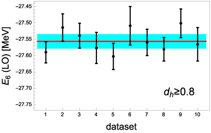

As for 12C, we have also studied the stability of the extrapolated results for as successive data points in the vicinity of are omitted. These results are summarized in Table 2, and the behavior of the extrapolated LO energy is illustrated in Fig. 11. Our findings suggest that a satisfactory extrapolation can be obtained as long as PMC calculations can be performed for values no smaller than , at least for the present range of coupling constants employed in the analysis. We note that a larger range in may allow smaller values of to serve as a useful starting point for the extrapolation, especially if the linear region around is thereby expanded. These findings appear consistent with our conclusions for 12C.
In contrast to performing extrapolations from SSE data below a given value of , we can instead perform linear fits to SSE data above a given . Such an analysis can demonstrate in what range of a linear description remains valid in the vicinity of . For this purpose, we perform linear fits for all possible combinations of three subsets (of the five total). This provides ten different possible datasets. We then choose a value of below which all data is discarded, and perform a linear extrapolation to the remaining data points. In fig. 11, we show the extrapolated LO results for and . We also show the average of the fits and corresponding 90% confidence bands. For the analysis with , our average is consistent with the complete LO extrapolation shown in Table 2, while for the analysis with , a clear systematical error is found. This shows (at least for 6He) that a linear description is valid for .
As an explicit demonstration of the amelioration of the sign problem using the SSE method, we show in Fig. 12 for the dependence of the mean value of the exponential of the complex phase of the PMC calculation on the number of Euclidean time steps and the SSE parameter for MeV-2. For the case of , the mean value quickly approaches zero as is increased, indicating that the sign problem is becoming severe at rather modest Euclidean projection times. For decreasing values of , the effect of the sign problem is successively diminished, allowing the PMC method to be extended to significantly larger values of .

V Discussion
The SSE method introduced here is inspired by the existence of an SU(4) symmetric Hamiltonian which provides a reasonably accurate description of the physics of the full Chiral EFT Hamiltonian. This has already proven useful in earlier work, as it greatly facilitates finding an accurate initial wave function which minimizes the extent of Euclidean time projection necessary with the full Hamiltonian. We have here illustrated how this concept can be taken one step further, by studying a weighted sum of physical and SU(4) symmetric Hamiltonians. In this way, the sign problem could be arbitrarily ameliorated, at the price of introducing an extrapolation in a control parameter . In practice, this means that the SSE method is only useful as long as the extrapolation errors can be kept under control. Naturally, performing simulations at a range of values of has the potential to multiply the required CPU time by a large factor. However, we have found that we are able to avoid an exponential increase in computation time as a function of Euclidean projection time, as long as we are able to perform simulations for , as the accuracy of extrapolation then remains comparable with the statistical errors of typical simulations at . We have also explored the freedom in the choice of the SU(4) symmetric Hamiltonian, which clearly plays no role at , but which in general gives different results for . We have therefore made use of a “triangulation” method to improve the accuracy of the extrapolation .
An important consideration is whether a continuous shift from an SU(4) symmetric Hamiltonian to the full Chiral EFT Hamiltonian can be effected without inducing non-trivial changes in the spectrum. For instance, the appearance of a level crossing at a critical value of would clearly limit the applicability of SSE. We note that such level crossings as a function of would be quite rare for low-lying nuclear bound states, and furthermore we have the freedom to choose to avoid such level crossings. But if a level crossing were to occur, there would be some subtleties in obtaining accurate and converged results. For such cases, it would be preferable to take the limit first, followed by extrapolation in Euclidean time. An even better solution would entail solving a coupled-channel problem using multiple initial states. This makes it possible to disentangle one or more nearly degenerate states with the same quantum numbers. So far, we have concentrated on systems where such degeneracies are not expected, and where PMC is still possible (though difficult) without the SSE method. We have also not yet explored different ”extrapolation Hamiltonians”, where the sign oscillations are minimized while retaining as much as possible of the full Chiral EFT structure.
In this first report on the SSE method, we have presented extensive results for 6He and 12C, for a wide range of and SU(4) symmetric Hamiltonians. For the case of 6He, we have first extrapolated all results to infinite Euclidean time, followed by an extrapolation . For the case of 12C, we have performed the extrapolation directly for data at finite Euclidean projection time. In both cases, we find similar behavior as a function of and excellent linearity in the vicinity of . Which ordering of the limits is preferable depends on how severe the sign problem is for a given system at . In cases where the sign problem is severe, the method of first taking the limit followed by an extrapolation in Euclidean time is preferable. This is because the Euclidean time extrapolation may be ambiguous if only very short Euclidean times are accessible with PMC. Our results provide the first determination of the ground state energy of 6He using lattice Chiral EFT, and for 12C we find that our new results at larger Euclidean projection time agree very well with previous infinite-time extrapolations.
We have presented here the first studies of the binding energy of 6He within lattice Chiral EFT. While the results are very encouraging for the feasibility of calculations for neutron-rich systems, we also find that 6He appears underbound by MeV at NNLO. Nevertheless, since the present calculations are performed in an box, the possibility remains that finite volume effects could significantly improve on the current situation. In particular, since -wave states are underbound in a finite volume [26, 27] while -wave states are overbound, calculations in larger boxes (or extrapolations to ) would shed more light on this situation.
We acknowledge partial financial support from the Deutsche Forschungsgemeinschaft (Sino-German CRC 110), the Helmholtz Association (Contract No. VH-VI-417), BMBF (Grant No. 05P12PDFTE), and the U.S. Department of Energy (DE-FG02-03ER41260). Further support was provided by the EU HadronPhysics3 project and the ERC Project No. 259218 NUCLEAREFT. The computational resources were provided by the Jülich Supercomputing Centre at Forschungszentrum Jülich and by RWTH Aachen. TL acknowledges financial support from the Magnus Ehrnrooth Foundation of the Finnish Society of Sciences and Letters.
References
- [1] D. Lee, B. Borasoy and T. Schäfer, “Nuclear lattice simulations with chiral effective field theory,” Phys. Rev. C 70 (2004) 014007 [nucl-th/0402072].
- [2] B. Borasoy, E. Epelbaum, H. Krebs, D. Lee and Ulf-G. Meißner, “Lattice Simulations for Light Nuclei: Chiral Effective Field Theory at Leading Order,” Eur. Phys. J. A 31 (2007) 105 [nucl-th/0611087].
- [3] B. Borasoy, E. Epelbaum, H. Krebs, D. Lee and Ulf-G. Meißner, “Chiral effective field theory on the lattice at next-to-leading order,” Eur. Phys. J. A 35 (2008) 343 [arXiv:0712.2990 [nucl-th]].
- [4] E. Epelbaum, H. Krebs, D. Lee and Ulf-G. Meißner, “Lattice chiral effective field theory with three-body interactions at next-to-next-to-leading order,” Eur. Phys. J. A 41 (2009) 125 [arXiv:0903.1666 [nucl-th]].
- [5] D. Lee, “Lattice simulations for few- and many-body systems,” Prog. Part. Nucl. Phys. 63 (2009) 117 [arXiv:0804.3501 [nucl-th]].
- [6] E. Epelbaum, H. Krebs, D. Lee and Ulf-G. Meißner, “Lattice effective field theory calculations for A = 3,4,6,12 nuclei,” Phys. Rev. Lett. 104 (2010) 142501 [arXiv:0912.4195 [nucl-th]].
- [7] E. Epelbaum, H. Krebs, D. Lee and Ulf-G. Meißner, “Lattice calculations for A=3,4,6,12 nuclei using chiral effective field theory,” Eur. Phys. J. A 45 (2010) 335 [arXiv:1003.5697 [nucl-th]].
- [8] T. A. Lähde, E. Epelbaum, H. Krebs, D. Lee, Ulf-G. Meißner and G. Rupak, “Lattice Effective Field Theory for Medium-Mass Nuclei,” Phys. Lett. B 732 (2014) 110 [arXiv:1311.0477 [nucl-th]].
- [9] T. A. Lähde, E. Epelbaum, H. Krebs, D. Lee, Ulf-G. Meißner and G. Rupak, “Lattice effective field theory for nuclei from A = 4 to A = 28,” PoS LATTICE 2013 (2014) 231 [arXiv:1311.1968 [nucl-th]].
- [10] B. Borasoy, E. Epelbaum, H. Krebs, D. Lee and Ulf-G. Meißner, “Dilute neutron matter on the lattice at next-to-leading order in chiral effective field theory,” Eur. Phys. J. A 35 (2008) 357 [arXiv:0712.2993 [nucl-th]].
- [11] E. Epelbaum, H. Krebs, D. Lee and Ulf-G. Meißner, “Ground state energy of dilute neutron matter at next-to-leading order in lattice chiral effective field theory,” Eur. Phys. J. A 40 (2009) 199 [arXiv:0812.3653 [nucl-th]].
- [12] E. Epelbaum, H. Krebs, T. A. Lähde, D. Lee and Ulf-G. Meißner, “Structure and rotations of the Hoyle state,” Phys. Rev. Lett. 109 (2012) 252501 [arXiv:1208.1328 [nucl-th]].
- [13] E. Epelbaum, H. Krebs, T. A. Lähde, D. Lee, Ulf-G. Meißner and G. Rupak, “Ab Initio Calculation of the Spectrum and Structure of 16O,” Phys. Rev. Lett. 112 (2014) 10, 102501 [arXiv:1312.7703 [nucl-th]].
- [14] T. A. Lähde, E. Epelbaum, H. Krebs, D. Lee, Ulf-G. Meißner and G. Rupak, “The Hoyle state in nuclear lattice effective field theory,” Pramana 83 (2014) 5, 651 [arXiv:1403.5451 [nucl-th]].
- [15] E. Epelbaum, H. Krebs, T. A. Lähde, D. Lee and Ulf-G. Meißner, “Viability of Carbon-Based Life as a Function of the Light Quark Mass,” Phys. Rev. Lett. 110 (2013) 11, 112502 [arXiv:1212.4181 [nucl-th]].
- [16] E. Epelbaum, H. Krebs, T. A. Lähde, D. Lee and Ulf-G. Meißner, “Dependence of the triple-alpha process on the fundamental constants of nature,” Eur. Phys. J. A 49 (2013) 82 [arXiv:1303.4856 [nucl-th]].
- [17] E. Wigner, “On the Consequences of the Symmetry of the Nuclear Hamiltonian on the Spectroscopy of Nuclei,” Phys. Rev. 51 (1937) 106.
- [18] D. B. Kaplan and M. J. Savage, “The Spin flavor dependence of nuclear forces from large n QCD,” Phys. Lett. B 365 (1996) 244 [hep-ph/9509371].
- [19] T. Mehen, I. W. Stewart and M. B. Wise, “Wigner symmetry in the limit of large scattering lengths,” Phys. Rev. Lett. 83 (1999) 931 [hep-ph/9902370].
- [20] D. Lee, “Inequalities for low-energy symmetric nuclear matter,” Phys. Rev. C 70, 064002 (2004) [nucl-th/0407088].
- [21] J. W. Chen, D. Lee and T. Schäfer, “Inequalities for light nuclei in the Wigner symmetry limit,” Phys. Rev. Lett. 93, 242302 (2004) [nucl-th/0408043].
- [22] D. Lee, “Spectral convexity for attractive SU(2N) fermions,” Phys. Rev. Lett. 98, 182501 (2007) [nucl-th/0701041].
- [23] Y. Alhassid, D. J. Dean, S. E. Koonin, G. Lang and W. E. Ormand, “Practical solution to the Monte Carlo sign problem: Realistic calculations of Fe-54,” Phys. Rev. Lett. 72, 613 (1994) [nucl-th/9310026].
- [24] S. E. Koonin, D. J. Dean and K. Langanke, “Shell model Monte Carlo methods,” Phys. Rept. 278, 1 (1997) [nucl-th/9602006].
- [25] T. A. Lähde, E. Epelbaum, H. Krebs, D. Lee, Ulf-G. Meißner and G. Rupak, “Uncertainties of Euclidean Time Extrapolation in Lattice Effective Field Theory,” J. Phys. G: Nucl. Part. Phys. 42 (2015) 034012 [arXiv:1409.7538 [nucl-th]].
- [26] S. König, D. Lee and H.-W. Hammer, “Volume Dependence of Bound States with Angular Momentum,” Phys. Rev. Lett. 107 (2011) 112001 [arXiv:1103.4468 [hep-lat]].
- [27] S. König, D. Lee and H.-W. Hammer, “Non-relativistic bound states in a finite volume,” Annals Phys. 327 (2012) 1450 [arXiv:1109.4577 [hep-lat]].