跳到论文正文
W Papers独立论文阅读器 arXiv:1502.06694 论文正文 计算阅读时间 · 0%
引用这篇论文根据当前论文元数据生成,正式投稿前建议核对。


License: arXiv.org perpetual non-exclusive license
arXiv:1502.06694v3 [math.DS] 30 Mar 2015

Robust Asymptotic Stability of Desynchronization in Impulse Coupled Oscillators Sean Phillips seaphill@ucsc.edu Ricardo G. Sanfelice ricardo@ucsc.edu August 24, 2026  Technical Report Hybrid Systems Laboratory Department of Computer Engineering University of California, Santa Cruz Technical Report No. arXivTR-HSL-001-2015
Available at https://hybrid.soe.ucsc.edu/biblio
Readers of this material have the responsibility to inform all of the authors promptly if they wish to reuse, modify, correct, publish, or distribute any portion of this report.

Abstract

The property of desynchronization in an all-to-all network of homogeneous impulse-coupled oscillators is studied. Each impulse-coupled oscillator is modeled as a hybrid system with a single timer state that self-resets to zero when it reaches a threshold, at which event all other impulse-coupled oscillators adjust their timers following a common reset law. In this setting, desynchronization is considered as each impulse-coupled oscillator’s timer having equal separation between successive resets. We show that, for the considered model, desynchronization is an asymptotically stable property. For this purpose, we recast desynchronization as a set stabilization problem and employ Lyapunov stability tools for hybrid systems. Furthermore, several perturbations are considered showing that desynchronization is a robust property. Perturbations on both the continuous and discrete dynamics are considered. Numerical results are presented to illustrate the main contributions.

1 Introduction

Impulse-coupled oscillators are multi-agent systems with state variables consisting of timers that evolve continuously until a state-dependent event triggers an instantaneous update of their values. Networks of such oscillators have been employed to model the dynamics of a wide range of biological and engineering systems. In fact, impulse-coupled oscillators have been used to model groups of fireflies [1], spiking neurons [2, 3], muscle cells [4], wireless networks [5], and sensor networks [6]. With synchronization being a property of particular interest, such complex networks have been found to coordinate the values of their state variables by sharing information only at the times the events/impulses occur [1, 7].

The opposite of synchronization is desynchronization. In simple words, desynchronization in multi-agent systems is the notion that the agents’ periodic actions are separated “as far apart” as possible in time. Desynchronization is similar to clustering or splay-state configurations, and is sometimes referred in the literature as inhibited behavior [8, 9]. For impulse-coupled oscillators, desynchronization is given as the behavior in which the separation between all of the timers impulses is equal [10]. This behavior has been found to be present in communication schemes in fish [11] and in networks of spiking neurons [12, 13]. Desynchronization of oscillators has recently been shown to be of importance in the understanding of Parkinson’s disease [14, 15], in the design of algorithms that limit the amount of overlapping data transfer and data loss in wireless digital networks [5], and in the design of round-robin scheduling schemes for sensor networks [6].

Motivated by the applications mentioned above and the lack of a full understanding of desynchronization in multi-agent systems, this paper pertains to the study of the dynamical properties of desynchronization in a network of impulse-coupled oscillators with an all-to-all communication graph. The uniqueness of the approach emerges from the use of hybrid systems tools, which not only conveniently capture the continuous and impulsive behavior in the networks of interest, but also are suitable for analytical study of asymptotic stability and robustness to perturbations.

More precisely, the dynamics of the proposed hybrid system capture the (linear) continuous evolution of the states as well their impulsive/discontinuous behavior due to state triggered events. Analysis of the asymptotic behavior of the trajectories (or solutions) to these systems is performed using the framework of hybrid systems introduced in [16, 17]. To this end, we recast the study of desynchronization as a set stabilization problem. Unlike synchronization, for which the set of points to stabilize is obvious, the complexity of desynchronization requires first to determine such a collection of points, which we refer to as the desynchronization set. We propose an algorithm to compute such set of points. Then, using Lyapunov stability theory for hybrid systems, we prove that the desynchronization set is asymptotically stable by defining a Lyapunov-like function as the distance between the state and (an inflated version of) the desynchronization set. In our context, asymptotic stability of the desynchronization set implies that the distance between the state and the desynchronization set converges to zero as the amount of time and the number of jumps get large. Using the proposed Lyapunov-like function and invoking an invariance principle, the basin of attraction is characterized and shown to be the entire state space minus a set of measure zero, which turns out to actually be an exact estimate of the basin of attraction. Furthermore, also exploiting the availability of a Lyapunov-like function, we analytically characterize the time for the solutions to reach a neighborhood of the desynchronization set. In particular, this characterization provides key insight for the design of algorithms used in applications in which desynchronization is crucial, such as wireless digital networks and sensor networks.

The asymptotic stability property of the desynchronization configuration is shown to be robust to several types of perturbations. The perturbations studied here include a generic perturbation in the form of an inflation of the dynamics of the proposed hybrid system model of the network of interest and several kinds of perturbations on the timer rates. Using the tools presented in [16, 17], we analytically characterize the effect of these perturbations on the already established asymptotic stability property of the desynchronization set. In particular, these perturbations capture situations where the agents in the network are heterogeneous due to having differing timer rates, threshold values, and update laws. To verify the analytical results, we simulate networks of impulse-coupled oscillators under several classes of perturbations. Specifically, we show numerical results when perturbations affect the update laws and the timer rates.

The remainder of this paper is organized as follows. Section 2 is devoted to hybrid modeling of networks of impulse-coupled oscillators. Section 3.1 introduces an algorithm to determine the desynchronization set. Section 3.2 presents the stability results while the time to convergence is characterized in Section 3.3. The robustness results are in Section 3.4. Section 4 presents numerical results illustrating our results. Final remarks are given in Section 5.

Notation

  • •

    ℝ\mathbb{R} denotes the space of real numbers.

  • •

    ℝn\mathbb{R}^{n} denotes the nn-dimensional Euclidean space.

  • •

    ℕ\mathbb{N} denotes the natural numbers including zero, i.e., ℕ={0,1,2,…}\mathbb{N}=\{0,1,2,...\}.

  • •

    For an interval 𝒦=[0,1]\mathcal{K}=[0,1] and n∈ℕ∖{0}n\in\mathbb{N}\setminus\{0\}, 𝒦n\mathcal{K}_{n} is the nn-product of the interval 𝒦\mathcal{K}, i.e., 𝒦n=[0,1]×[0,1]×…×[0,1]\mathcal{K}_{n}=[0,1]\times[0,1]\times\ldots\times[0,1].

  • •

    𝔹\mathbb{B} is the closed unit ball centered around the origin in Euclidean space.

  • •

    𝟏\mathbf{1} is an NN column vector of ones.

  • •

    𝟏¯\underline{\mathbf{1}} is an N×NN\times N matrix full of ones.

  • •

    𝐈{\bf I} is the N×NN\times N identity matrix.

  • •

    Given a closed set 𝒜⊂ℝn\mathcal{A}\subset\mathbb{R}^{n} and x∈ℝnx\in\mathbb{R}^{n}, |x|𝒜:=minz∈𝒜⁡|x−z||x|_{\mathcal{A}}:=\min_{z\in\mathcal{A}}|x-z|.

  • •

    Given x∈ℝnx\in\mathbb{R}^{n}, |x||x| denotes the Euclidean norm of xx.

  • •

    The cc-level set of V:domV→ℝV:\mathop{\rm dom}\nolimits V\to\mathbb{R} is given by LV​(c):={x∈domV:V⁡(x)=c}L_{V}(c):=\{x\in\mathop{\rm dom}\nolimits V:V(x)=c\},

2 Hybrid System Model of Impulse-Coupled Oscillators

2.1 Mathematical Model

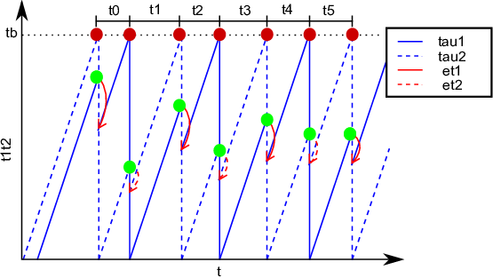
In this paper, we consider a model of NN impulse-coupled oscillators. Each impulse-coupled oscillator has a continuous state (τi\tau_{i} for the ii-th oscillator) defining its internal timer. Once the timer of any oscillator reaches a threshold (τ¯\bar{\tau}), it triggers an impulse and is reset to zero. At such an event, all the other impulse-coupled oscillators rescale their timer by a factor given by (1+ε)(1+\varepsilon) times the value of their timer, where ε∈(−1,0)\varepsilon\in(-1,0).11 1 Cf. the model for synchronization in [1] where ε>0\varepsilon>0. Figure 1 shows a trajectory of two impulse-coupled oscillators with states τ1\tau_{1} and τ2\tau_{2}. In this figure, the dark red circles indicate when a timer state has reached the threshold and, thus, resets to zero. The light green circles indicate when an oscillator is externally reset and, hence, decreases its timer by (1+ε)(1+\varepsilon) times its current state.

Refer to caption
Figure 1: An example of two impulse-coupled oscillators reaching desynchronization (as Δ​ti\Delta t_{i} converges to a constant.) The internal resets ( dark red circles) map the timers to zero. The external resets ( light green circles) map the timers to a fraction (1+ε)(1+\varepsilon) of their current value.

According to this outline of the model, the dynamics of the impulse-coupled oscillators involve impulses and timer resets, which are treated as true discrete events and instantaneous updates, while the smooth evolution of the timers before/after these events define the continuous dynamics. We follow the hybrid formalism of [16, 17], where a hybrid system is given by four objects (C,f,D,G)(C,f,D,G) defining its data:

  • •

    Flow set: a set C⊂ℝNC\subset\mathbb{R}^{N} specifying the points where flows are possible (or continuous evolution).

  • •

    Flow map: a single-valued map f:ℝN→ℝNf:\mathbb{R}^{N}\to\mathbb{R}^{N} defining the flows.

  • •

    Jump set: a set D⊂ℝND\subset\mathbb{R}^{N} specifying the points where jumps are possible (or discrete evolution).

  • •

    Jump map: a set-valued map G:ℝN⇉ℝNG:\mathbb{R}^{N}\rightrightarrows\mathbb{R}^{N} defining the jumps.

A hybrid system capturing the dynamics of the impulse-coupled oscillators is denoted as ℋN:=(C,f,D,G){\mathcal{H}}_{N}:=(C,f,D,G) and can be written in the compact form

ℋN:τ∈ℝN{τ˙=f⁡(τ)τ∈Cτ+∈G⁡(τ)τ∈D,{\mathcal{H}}_{N}:\qquad\tau\in\mathbb{R}^{N}\qquad\left\{\begin{array}[]{llll}\dot{\tau}&=&f(\tau)&\quad\tau\in C\\ \tau^{+}&\in&G(\tau)&\quad\tau\in D\end{array}\right., (1)

where N∈ℕ∖{0,1}N\in\mathbb{N}\setminus\{0,1\} is the number of impulse-coupled oscillators. The state of ℋN{\mathcal{H}}_{N} is given by

τ:=[τ1τ2…τN]⊤∈PN:=[0,τ¯]N.\tau:=\left[\tau_{1}\ \ \tau_{2}\ \ \ldots\ \ \tau_{N}\right]^{\top}\in P_{N}:=[0,\bar{\tau}]^{N}.

The flow and jump sets are defined to constrain the evolution of the timers. The flow set is defined by

C:=PN,\color[rgb]{0,0,0}C:=P_{N},\color[rgb]{0,0,0} (2)

where I:={1,2,…,N}I:=\{1,2,\ldots,N\} and τ¯>0\bar{\tau}>0 is the threshold. During flows, an internal clock gradually increases based on the homogeneous rate, ω\omega. Then, the flow map is defined as

f⁡(τ):=ω​𝟏∀τ∈Cf(\tau):=\omega\mathbf{1}\qquad\forall\tau\in C

with ω>0\omega>0 defining the natural frequency of each impulse-coupled oscillator. The impulsive events are captured by a jump set DD and a jump map GG. Jumps occur when the state is in the jump set DD defined as

D:={τ∈PN:∃i∈I​s.t.​τi=τ¯}.D:=\left\{\tau\in P_{N}:\ \exists i\in I\ \mbox{s.t.}\ \tau_{i}=\bar{\tau}\right\}. (3)

From such points, the ii-th timer is reset to zero and forces a jump of all other timers. Such discrete dynamics are captured by the following jump map: for each τ∈D\tau\in D define G⁡(τ)=[g1​(τ)g2​(τ)…gN​(τ)]⊤,G(\tau)=\left[g_{1}(\tau)\ \ g_{2}(\tau)\ \ \ldots\ \ g_{N}(\tau)\right]^{\top}, where, for each i∈Ii\in I,

gi​(τ)={0if ​τi=τ¯,τr<τ¯∀r∈I∖{i}{0,τi​(1+ε)}​if ​τi=τ¯​∃r∈I∖{i}​s.t.​τr=τ¯(1+ε)​τiif ​τi<τ¯​∃r∈I∖{i}​s.t.​τr=τ¯g_{i}(\tau)=\left\{\begin{array}[]{l}0\qquad\qquad\ \ \ \ \mbox{if }\tau_{i}=\bar{\tau},\tau_{r}<\bar{\tau}\ \ \forall r\in I\setminus\{i\}\\ \{0,\tau_{i}(1+\varepsilon)\}\ \mbox{if }\tau_{i}=\bar{\tau}\ \exists r\in I\setminus\{i\}\ \mbox{s.t.}\ \tau_{r}=\bar{\tau}\\ (1+\varepsilon)\tau_{i}\qquad\ \mbox{if }\tau_{i}<\bar{\tau}\ \exists r\in I\setminus\{i\}\ \mbox{s.t.}\ \tau_{r}=\bar{\tau}\end{array}\right. (4)

with parameters ε∈(−1,0)\varepsilon\in(-1,0) and τ¯>0\bar{\tau}>0; for τ∈D\tau\in D, gig_{i} is not empty. When a jump is triggered, the state τi\tau_{i} jumps according to the ii-th component of the jump map gig_{i}. When a state reaches the threshold τ¯\bar{\tau}, it is reset to zero only when all other states are less than that threshold; otherwise, if multiple timers reach the threshold simultaneously, the jump map is set valued to indicate that either gi​(τ)=0g_{i}(\tau)=0 or gi​(τ)=(1+ε)​τig_{i}(\tau)=(1+\varepsilon)\tau_{i} is possible. This is to ensure that the jump map satisfies the regularity conditions outlined in Section 2.2.22 2 In [8], a more general flow map and a jump map incrementing τi\tau_{i} by ε>0\varepsilon>0 are considered.

For example, consider the case N=2N=2 the hybrid system ℋN=(C,f,D,G){\mathcal{H}}_{N}=(C,f,D,G) has state given by

τ=[τ1τ2]∈P2:=[0,τ¯]×[0,τ¯].\tau=\left[\begin{array}[]{c}\tau_{1}\\ \tau_{2}\end{array}\right]\in P_{2}:=[0,\bar{\tau}]\times[0,\bar{\tau}].

The states τ1\tau_{1} and τ2\tau_{2} are the timers for both of the oscillators. The hybrid system ℋ2{\mathcal{H}}_{2} has the following data:

ℋ2={C=P2,f⁡(τ)=[11]​∀τ∈C,D={τ∈P2:∃i∈{1,2}s.t.τi=τ¯},G⁡(τ)=[g1​(τ)g2​(τ)]​∀τ∈D,{\mathcal{H}}_{2}=\left\{\begin{array}[]{ll}C=P_{2},&\qquad f(\tau)=\left[\begin{array}[]{c}1\\ 1\end{array}\right]\forall\tau\in C,\\ \vskip 6.0pt plus 2.0pt minus 2.0pt\cr D=\left\{\tau\in P_{2}\ :\ \exists i\in\{1,2\}\ s.t.\ \tau_{i}=\bar{\tau}\right\},&\qquad G(\tau)=\left[\begin{array}[]{c}g_{1}(\tau)\\ g_{2}(\tau)\end{array}\right]\forall\tau\in D,\end{array}\right.

where the functions g1g_{1} and g2g_{2} are defined as

g1​(τ)={0if ​τ1=τ¯,τ2<τ¯{0,τ1​(1+ε)}if ​τ1=τ¯,τ2=τ¯(1+ε)​τ1if ​τ1<τ¯,τ2=τ¯g2​(τ)={0if ​τ2=τ¯,τ1<τ¯{0,τ2​(1+ε)}if ​τ2=τ¯,τ1=τ¯(1+ε)​τ2if ​τ2<τ¯,τ1=τ¯.g_{1}(\tau)=\left\{\begin{array}[]{ll}0&\mbox{if }\tau_{1}=\bar{\tau},\tau_{2}<\bar{\tau}\\ \{0,\tau_{1}(1+\varepsilon)\}&\mbox{if }\tau_{1}=\bar{\tau},\tau_{2}=\bar{\tau}\\ (1+\varepsilon)\tau_{1}&\mbox{if }\tau_{1}<\bar{\tau},\tau_{2}=\bar{\tau}\end{array}\right.\qquad\qquad g_{2}(\tau)=\left\{\begin{array}[]{ll}0&\mbox{if }\tau_{2}=\bar{\tau},\tau_{1}<\bar{\tau}\\ \{0,\tau_{2}(1+\varepsilon)\}&\mbox{if }\tau_{2}=\bar{\tau},\tau_{1}=\bar{\tau}\\ (1+\varepsilon)\tau_{2}&\mbox{if }\tau_{2}<\bar{\tau},\tau_{1}=\bar{\tau}\end{array}\right..

2.2 Basic Properties of ℋN{\mathcal{H}}_{N}

2.2.1 Hybrid Basic Conditions

To apply analysis tools for hybrid systems in [16], which will be summarized in Section 3, the data of the hybrid system ℋN{\mathcal{H}}_{N} must meet certain mild conditions. These conditions, referred to as the hybrid basic conditions, are as follows:

  1. A1)

    CC and DD are closed sets in ℝN\mathbb{R}^{N}.

  2. A2)

    f:ℝN→ℝNf:\mathbb{R}^{N}\to\mathbb{R}^{N} is continuous on CC.

  3. A3)

    G:ℝN⇉ℝNG:\mathbb{R}^{N}\rightrightarrows\mathbb{R}^{N} is an outer semicontinuous33 3 A set-valued mapping G:ℝN⇉ℝNG:\mathbb{R}^{N}\rightrightarrows\mathbb{R}^{N} is outer semicontinuous if its graph {(x,y):x∈ℝN,y∈G(x)}\{(x,y):x\in\mathbb{R}^{N},y\in G(x)\} is closed, see [16, Lemma 5.10] and [18]. set-valued mapping, locally bounded on DD, and such that G⁡(x)G(x) is nonempty for each x∈Dx\in D.

Lemma 2.1

ℋN{\mathcal{H}}_{N} satisfies the hybrid basic conditions.

Condition (A1) is satisfied since CC and DD are closed. The function ff is constant and therefore continuous on CC, satisfying (A2). With GG as in (4), the graph of each gig_{i} is defined as

gph​(gi)\displaystyle\mbox{gph}(g_{i}) ={(x,y):y∈gi(x),x∈D}\displaystyle=\{(x,y):y\in g_{i}(x),x\in D\}
={(x,y):y=0,xi=τ¯,xr≤τ¯∀r≠i,x∈D}∪{(x,y):y=(1+ε)xi,xi≤τ¯∃xr=τ¯,x∈D}\displaystyle=\{(x,y):y=0,x_{i}=\bar{\tau},x_{r}\leq\bar{\tau}\ \forall r\neq i,x\in D\}\cup\{(x,y):y=(1+\varepsilon)x_{i},x_{i}\leq\bar{\tau}\ \exists x_{r}=\bar{\tau},x\in D\}

which is closed. Then the set-valued mapping GG is outer semicontinuous. By definition, GG is bounded and nonempty for each τ∈D\tau\in D, and hence it satisfies (A3). ■\blacksquare

Note that satisfying the hybrid basic conditions implies that ℋN{\mathcal{H}}_{N} is well-posed [16, Theorem 6.30], which automatically gives robustness to vanishing state disturbances; see [16, 17]. Section 3.4 considers different types of perturbations that ℋN{\mathcal{H}}_{N} can withstand.

2.2.2 Solutions to ℋN{\mathcal{H}}_{N}

Solutions to generic hybrid systems ℋ{\mathcal{H}} with state x∈ℝnx\in\mathbb{R}^{n} will be given by hybrid arcs on hybrid time domains defined as follows:

Definition 2.2

(hybrid time domain) A subset S⊂ℝ≥0×ℕS\subset{\mathbb{R}_{\geq 0}}\times\mathbb{N} is a compact hybrid time domain if

S=⋃j=0J−1([tj,tj+1],j)S=\bigcup_{j=0}^{J-1}\left([t_{j},t_{j+1}],j\right)

for some finite sequence of times 0=t0≤t1≤t2​…≤tJ0=t_{0}\leq t_{1}\leq t_{2}\ ...\leq t_{J}. A subset S⊂ℝ≥0×ℕS\subset{\mathbb{R}_{\geq 0}}\times\mathbb{N} is a hybrid time domain if for all (T,J)∈S(T,J)\in S, S∩([0,T]×{0,1,…​J})S\ \cap\ \left([0,T]\times\{0,1,...J\}\right) is a compact hybrid time domain.

Definition 2.3

(hybrid arc) A function x:domx→ℝnx:\mathop{\rm dom}\nolimits x\to\mathbb{R}^{n} is a hybrid arc if domx\mathop{\rm dom}\nolimits x is a hybrid time domain and if for each j∈ℕj\in\mathbb{N}, the function t↦x⁡(t,j)t\mapsto x(t,j) is locally absolutely continuous.

Definition 2.4

(solution) A hybrid arc xx is a solution to the hybrid system ℋ{\mathcal{H}} if x⁡(0,0)∈C∪Dx(0,0)\in C\cup D and:

  1. (S1)

    For all j∈ℕj\in\mathbb{N} and almost all tt such that (t,j)∈domx(t,j)\in\mathop{\rm dom}\nolimits x,

    x⁡(t,j)∈C,x˙​(t,j)=f⁡(x⁡(t,j)).x(t,j)\in C,\ \ \ \dot{x}(t,j)=f(x(t,j))\ .
  2. (S2)

    For all (t,j)∈domx(t,j)\in\mathop{\rm dom}\nolimits x such that (t,j+1)∈domx(t,j+1)\in\mathop{\rm dom}\nolimits x,

    x⁡(t,j)∈D,x⁡(t,j+1)∈G⁡(x⁡(t,j)).x(t,j)\in D,\ \ \ x(t,j+1)\in G(x(t,j))\ .

A solution xx is said to be nontrivial if domx\mathop{\rm dom}\nolimits x contains at least one point different from (0,0)(0,0), maximal if there does not exist a solution x′x^{\prime} such that xx is a truncation of x′x^{\prime} to some proper subset of domx′\mathop{\rm dom}\nolimits x^{\prime}, complete if domx\mathop{\rm dom}\nolimits x is unbounded, and Zeno if it is complete but the projection of domx\mathop{\rm dom}\nolimits x onto ℝ≥0{\mathbb{R}_{\geq 0}} is bounded.

Lemma 2.5

From every point in C∪DC\cup D, there exists a solution and every maximal solution to ℋN{\mathcal{H}}_{N} is complete and bounded.

The result follows from Proposition 2.10 in [16] using the following properties. For each point such that τ∈C\tau\in C, the components of the flow map ff are positive and induce solutions that flow towards DD. For each τ∈D\tau\in D, the jump map satisfies G⁡(τ)⊂CG(\tau)\subset C. Since it is impossible for solutions with initial conditions τ⁡(0,0)∈C∪D\tau(0,0)\in C\cup D to escape C∪DC\cup D, all maximal solutions are complete and bounded. ■\blacksquareDue to the jump map GG, if the elements of the solution are initially equal (denote this set as 𝒮:={τ∈PN:∃i,r∈I,i≠r,τi=τr}\mathcal{S}:=\{\tau\in P_{N}:\exists i,r\in I,i\neq r,\tau_{i}=\tau_{r}\}) it is possible for them to remain equal for all time. Furthermore, it is also possible for solutions to be initialized on the jump set such that one element is at the threshold and another is equal to zero then after the jump they will be equal, e.g. let τ1=τ¯\tau_{1}=\bar{\tau}, τ2=0\tau_{2}=0 then τ1+=τ2+=0\tau_{1}^{+}=\tau_{2}^{+}=0. We denote this set as 𝒢:={τ∈D∖𝒮:∃i,r∈I,i≠r,τi=0,τr=τ¯}\mathcal{G}:=\{\tau\in D\setminus\mathcal{S}:\exists i,r\in I,i\neq r,\tau_{i}=0,\tau_{r}=\bar{\tau}\}. The next result considers solutions initialized on the set 𝒳:=𝒮∪𝒢\mathcal{X}:=\mathcal{S}\cup\mathcal{G}.

Lemma 2.6

For each τ⁡(0,0)∈𝒳\tau(0,0)\in\mathcal{X}, there exists a solution τ\tau to ℋN{\mathcal{H}}_{N} from τ⁡(0,0)\tau(0,0) such that, for some M∈{0,1}M\in\{0,1\}, τ⁡(t,j)∈𝒮\tau(t,j)\in\mathcal{S} for all t+j≥Mt+j\geq M, (t,j)∈domτ(t,j)\in\mathop{\rm dom}\nolimits\tau.

Consider a solution τ\tau to the hybrid system ℋN{\mathcal{H}}_{N} with initial condition τ⁡(0,0)∈𝒮\tau(0,0)\in\color[rgb]{0,0,0}\mathcal{S}\color[rgb]{0,0,0}. Due to the flow map for each state being equal, τ\tau remains in 𝒮\mathcal{S} during flows. Furthermore, at points τ∈𝒮∩D\tau\in\mathcal{S}\cap D, the jump map GG is set valued by the definition of gig_{i} in (4). From these points, G⁡(τ)∩𝒮≠∅G(\tau)\cap\mathcal{S}\neq\emptyset. In fact, for each τ⁡(0,0)∈𝒮\tau(0,0)\in\mathcal{S}, there exists at least one solution such that τ⁡(t,j)∈𝒮\tau(t,j)\in\mathcal{S} for all t+j≥0t+j\geq 0, with (t,j)∈domτ(t,j)\in\mathop{\rm dom}\nolimits\tau. Consider the case of solutions initialized at τ⁡(0,0)∈𝒢\tau(0,0)\in\color[rgb]{0,0,0}\mathcal{G}\color[rgb]{0,0,0} (Note that τ⁡(0,0)∈D\tau(0,0)\in D). It follows that for some r∈Ir\in I, τr​(0,0)=τ¯\tau_{r}(0,0)=\bar{\tau} and gr​(τ⁡(0,0))=0g_{r}(\tau(0,0))=0. Therefore, after the initial jump, we have that G⁡(τ⁡(0,0))∩𝒮≠∅,G(\tau(0,0))\cap\mathcal{S}\neq\emptyset, by which using previous arguments implies that τ⁡(t,j)∈𝒮\tau(t,j)\in\mathcal{S} for all t+j≥1t+j\geq 1.

Furthermore, there is a distinct ordering to the jumps. If τ\tau is such that τi≠τr\tau_{i}\neq\tau_{r} for all i≠ri\neq r then the ordering of each τi\tau_{i} is preserved after NN jumps. More specifically, we have the following result.

Lemma 2.7

For every solution τ\tau to ℋN{\mathcal{H}}_{N} with τ⁡(0,0)∉𝒳\tau(0,0)\notin\mathcal{X}, if at (tj,j)∈domτ(t_{j},j)\in\mathop{\rm dom}\nolimits\tau we have

0≤τi1​(tj,j)<τi2​(tj,j)<…<τiN​(tj,j)≤τ¯0\leq\tau_{i_{1}}(t_{j},j)<\tau_{i_{2}}(t_{j},j)<...<\tau_{i_{N}}(t_{j},j)\leq\bar{\tau}

for some sequence of nonrepeated elements {im}m=1N\{i_{m}\}^{N}_{m=1} of II (that is, a reordering of the elements of the set I={1,2,…,N}I=\{1,2,\ldots,N\}) then, after NN jumps, it follows that

0≤τi1​(tj+N,j+N)<τi2​(tj+N,j+N)<…<τiN​(tj+N,j+N)≤τ¯.0\leq\tau_{i_{1}}(t_{j+N},j+N)<\tau_{i_{2}}(t_{j+N},j+N)<...<\tau_{i_{N}}(t_{j+N},j+N)\leq\bar{\tau}.

Let τ\tau be a solution to ℋN{\mathcal{H}}_{N} from PN∖𝒳P_{N}\setminus\mathcal{X}. There exists a sequence iki_{k} of distinct elements with ik∈Ii_{k}\in I for each k∈Ik\in I, such that 0≤τi1​(t,j)<τi2​(t,j)<…<τiN​(t,j)≤τ¯0\leq\tau_{i_{1}}(t,j)<\tau_{i_{2}}(t,j)<\ldots<\tau_{i_{N}}(t,j)\leq\bar{\tau} over [t0,t1]×{0}[t_{0},t_{1}]\times\{0\}. After the jump at (t,j)=(t1,0)(t,j)=(t_{1},0) we have 0=τiN​(t,j+1)<τi1​(t,j+1)<τi2​(t,j+1)<…<τiN−1​(t,j+1)<τ¯0=\tau_{i_{N}}(t,j+1)<\tau_{i_{1}}(t,j+1)<\tau_{i_{2}}(t,j+1)<\ldots<\tau_{i_{N-1}}(t,j+1)<\bar{\tau}. Continuing this way for each jump, it follows that after N−1N-1 more jumps, the solution is such that 0≤τi1​(tN,j+N)<τi2​(tN,j+N)<…<τiN​(tN,j+N)≤τ¯0\leq\tau_{i_{1}}(t_{N},j+N)<\tau_{i_{2}}(t_{N},j+N)<\ldots<\tau_{i_{N}}(t_{N},j+N)\leq\bar{\tau} and the order at time (t,j)(t,j) is preserved. Using these properties of solutions to ℋN{\mathcal{H}}_{N}, the next section defines the set to which these solutions converge and establishes its stability properties.

3 Dynamical Properties of ℋN{\mathcal{H}}_{N}

Our goal is to show that the desynchronization configuration of ℋN{\mathcal{H}}_{N}, which is defined in Section 3.1, is asymptotically stable. We recall from [16, 17] the following definition of asymptotic stability for general hybrid systems with state x∈ℝnx\in\mathbb{R}^{n}.

Definition 3.1 (stability)

A closed set 𝒜⊂ℝn\mathcal{A}\subset\mathbb{R}^{n} is said to be

  • •

    stable if for each ε>0\varepsilon>0 there exists δ>0\delta>0 such that each solution xx with |x⁡(0,0)|𝒜≤δ|x(0,0)|_{\mathcal{A}}\leq\delta satisfies |x⁡(t,j)|𝒜≤ε|x(t,j)|_{\mathcal{A}}\leq\varepsilon for all (t,j)∈domx(t,j)\in\mathop{\rm dom}\nolimits x;

  • •

    attractive if there exists μ>0\mu>0 such that every maximal solution xx with |x⁡(0,0)|𝒜≤μ|x(0,0)|_{\mathcal{A}}\leq\mu is complete and satisfies
    lim(t,j)∈domx,t+j→∞|x⁡(t,j)|𝒜=0\lim_{(t,j)\in\mathop{\rm dom}\nolimits x,t+j\to\infty}|x(t,j)|_{\mathcal{A}}=0;

  • •

    asymptotically stable if stable and attractive;

  • •

    weakly globally asymptotically stable if 𝒜\mathcal{A} is stable and if, for every initial condition, there exists a maximal solution that is complete and satisfies lim(t,j)∈domx,t+j→∞|x⁡(t,j)|𝒜=0\lim_{(t,j)\in\mathop{\rm dom}\nolimits x,t+j\to\infty}|x(t,j)|_{\mathcal{A}}=0.

The set of points from where the attractivity property holds is the basin of attraction and excludes all points where the system trajectories may never converge to 𝒜\mathcal{A}. In fact, it will be established in Section 3.2 that the basin of attraction for asymptotic stability of desynchronization of ℋN{\mathcal{H}}_{N} does not include any point τ\tau such that any two or more timers are equal or become equal after a jump, which is the set 𝒳\mathcal{X} defined in Lemma 2.6. For example, consider the case N=2N=2, i.e., ℋ2{\mathcal{H}}_{2}. Then, the set 𝒳2\mathcal{X}_{2} is defined as

𝒳2=𝒮2∪𝒢2=({τ∈P2:τ1=τ2})∪({τ∈D:g1​(τ)=τ2}∪{τ∈D:g2​(τ)=τ1}).\displaystyle\begin{split}\mathcal{X}_{2}&=\mathcal{S}_{2}\cup\mathcal{G}_{2}=\left(\{\tau\in P_{2}:\tau_{1}=\tau_{2}\}\right)\cup\left(\{\tau\in D:g_{1}(\tau)=\tau_{2}\}\cup\{\tau\in D:g_{2}(\tau)=\tau_{1}\}\right).\end{split} (5)

Note that the set 𝒮2\mathcal{S}_{2} defines the line τ1=τ2\tau_{1}=\tau_{2} in P2P_{2} and 𝒢2\mathcal{G}_{2} is given by the points {(0,τ¯),(τ¯,0)}\{(0,\bar{\tau}),(\bar{\tau},0)\} in P2P_{2}; see Figure 2(a). For N=3N=3, the set 𝒳3\mathcal{X}_{3} is defined as

𝒳3=𝒮3∪𝒢3\displaystyle\mathcal{X}_{3}=\mathcal{S}_{3}\cup\mathcal{G}_{3} (6)

where

𝒮3=\displaystyle\mathcal{S}_{3}= {τ∈P3:τ1=τ2}∪{τ∈P3:τ1=τ3}∪{τ∈P3:τ2=τ3}\displaystyle\{\tau\in P_{3}\ :\tau_{1}=\tau_{2}\}\cup\{\tau\in P_{3}\ :\tau_{1}=\tau_{3}\}\cup\{\tau\in P_{3}\ :\tau_{2}=\tau_{3}\} (7)

and

𝒢3={τ∈P3:g1​(τ)=τ3}∪{τ∈P3:g2​(τ)=τ1}∪{τ∈P3:g3​(τ)=τ1}∪{τ∈P3:g2​(τ)=τ3}∪{τ∈P3:g3​(τ)=τ2}∪{τ∈P3:g1​(τ)=τ2}.\displaystyle\begin{split}\mathcal{G}_{3}=&\{\tau\in P_{3}\ :g_{1}(\tau)=\tau_{3}\}\cup\{\tau\in P_{3}\ :g_{2}(\tau)=\tau_{1}\}\cup\{\tau\in P_{3}\ :g_{3}(\tau)=\tau_{1}\}\cup\{\tau\in P_{3}\ :g_{2}(\tau)=\tau_{3}\}\\ &\qquad\cup\{\tau\in P_{3}\ :g_{3}(\tau)=\tau_{2}\}\cup\{\tau\in P_{3}\ :g_{1}(\tau)=\tau_{2}\}.\end{split} (8)

Then, 𝒳3\mathcal{X}_{3} is defined by the union of 𝒮3\mathcal{S}_{3}, which is the as the union of the planes in P3P_{3} given by τ1=τ2\tau_{1}=\tau_{2}, τ1=τ3\tau_{1}=\tau_{3}, and τ2=τ3\tau_{2}=\tau_{3}, and 𝒢3\mathcal{G}_{3}, which is given by {(τ¯,τ2,0),(0,τ2,τ¯),(τ1,τ¯,0),(τ1,0,τ¯),(τ¯,0,τ3),(0,τ¯,τ3):τ∈P3}\{(\bar{\tau},\tau_{2},0),(0,\tau_{2},\bar{\tau}),(\tau_{1},\bar{\tau},0),\\ (\tau_{1},0,\bar{\tau}),(\bar{\tau},0,\tau_{3}),(0,\bar{\tau},\tau_{3}):\tau\in P_{3}\}; see Figure 3. For this purpose, a Lyapunov-like function be constructed in Section 3.2 to show that a compact set denoted 𝒜\mathcal{A}, defining the desynchronization condition, is asymptotically stable and weakly globally asymptotically stable.

Refer to caption
(a) The sets 𝒳2\mathcal{X}_{2} (dashed green) and 𝒜\mathcal{A} (solid blue and red). The set 𝒜\mathcal{A} is defined by the union of ℓ1\ell_{1} and ℓ2\ell_{2} (See Section 3.1).

Refer to caption
(b) A simulation (dashed blue) of ℋ2{\mathcal{H}}_{2} showing the attractivity of the set 𝒜\mathcal{A} (solid black).
Figure 2: Sets associated with ℋ2{\mathcal{H}}_{2} and a solution to it from τ⁡(0,0)=[0.7,0.75]⊤\tau(0,0)=[0.7,0.75]^{\top} with ε=0.3\varepsilon=0.3 and τ¯=1\bar{\tau}=1.
Refer to caption
Figure 3: Points in each blue plane and line belong to the set 𝒳3\mathcal{X}_{3}.

3.1 Construction of the set 𝒜\mathcal{A} for ℋN{\mathcal{H}}_{N}

In this section, we identify the set of points corresponding to the impulse-coupled oscillators being desynchronized, namely, we define the desynchronization set. We define desynchronization as the behavior in which the separation between all of the timers’ impulses is equal (and nonzero), see Figure 1. More specifically desynchronization is defined as follows:

Definition 3.2

A solution τ\tau to ℋN{\mathcal{H}}_{N} is desynchronized if there exists Δ>0\Delta>0 and a sequence of non-repeated elements {im}m=1N\{i_{m}\}^{N}_{m=1} of II (that is, a reordering of the elements of the set I={1,2,…,N}I=\{1,2,\ldots,N\}) such that limj→∞(tjim−tjim+1)=Δ\lim_{j\to\infty}(t_{j}^{i_{m}}-t_{j}^{i_{m+1}})=\Delta for all m∈{1,2,…,N−1}m\in\{1,2,\ldots,N-1\} and limj→∞(tjN−tji1)=Δ,\lim_{j\to\infty}(t_{j}^{N}-t_{j}^{i_{1}})=\Delta, where {tjim}j=0∞\{t_{j}^{i_{m}}\}_{j=0}^{\infty} is the sequence of jump times of the state τim\tau_{i_{m}}.

In fact, this separation between impulses leads to an ordered sequence of impulse times with equal separation. The desynchronization set 𝒜\mathcal{A} for the hybrid system ℋN{\mathcal{H}}_{N} captures such a behavior and is parameterized by ε\varepsilon, the threshold τ¯\bar{\tau}, and the number of impulse-coupled oscillators NN.

To define this set, first we provide some basic intuition about the dynamics of ℋN{\mathcal{H}}_{N} when desynchronized. The set 𝒜\mathcal{A} must be forward invariant and such that trajectories staying in it satisfy the property in Definition 3.2. Due to the definition of the flow map ff, there exist sets in the form of “lines” ℓk\ell_{k}, each of them in the direction 𝟏\mathbf{1}, which is the direction of the flow map, intersecting the jump set at a point which, for the kk-th line, we denote as τ~k\widetilde{\tau}^{k}. We define the desynchronization set as the union of sets ℓk\ell_{k} collecting points τ=τ~k+𝟏​s∈PN\tau=\widetilde{\tau}^{k}+\mathbf{1}s\in P_{N} parameterized by s∈ℝs\in\mathbb{R}. Figure 2(a) shows ℓ1\ell_{1} and ℓ2\ell_{2} (solid blue and red) for the case N=2N=2.

To identify τ~k\widetilde{\tau}^{k}, consider a point τ~k∈D∖𝒳\widetilde{\tau}^{k}\in D\setminus\mathcal{X} with components satisfying τ~1k=τ¯>τ~2k>τ~3k>…>τ~Nk\widetilde{\tau}_{1}^{k}=\bar{\tau}>\widetilde{\tau}_{2}^{k}>\widetilde{\tau}_{3}^{k}>...>\widetilde{\tau}_{N}^{k}. Due to Definition 3.2, it must be true that the difference between jump times are constant. This means that there must be some correlation between Δ\Delta and the difference between, in this case, τ1k\tau_{1}^{k} and τ2k\tau_{2}^{k}. Moreover, there must be a correlation between τ1k\tau_{1}^{k} and all other states at jumps. It follows that this point belongs to 𝒜\mathcal{A} only if the distance between the expiring timer (τ~1k\widetilde{\tau}_{1}^{k}) and each of its other components (τ~ik\widetilde{\tau}_{i}^{k}, i∈I∖{1}i\in I\setminus\{1\}) is equal to the distance between the value after the jump of the timer expiring next (τ~2k​+\widetilde{\tau}_{2}^{k}\hbox{}^{+}) and the value after the jump of its other components (τ~ik​+\widetilde{\tau}_{i}^{k}\hbox{}^{+}, i∈I∖{2}i\in I\setminus\{2\}), respectively. This property ensures that, when in the desynchronization set, the relative distance between the leading timer and each of the other timers is equal, before and after jumps. More precisely,

τ~1k−τ~ik=τ~2k​+−τ~next​(i)k​+∀i∈I∖{1},\displaystyle\widetilde{\tau}_{1}^{k}-\widetilde{\tau}_{i}^{k}=\widetilde{\tau}_{2}^{k}\hbox{}^{+}-\widetilde{\tau}_{\mbox{\scriptsize next}(i)}^{k}\hskip-15.17719pt\hbox{}^{+}\qquad\qquad\forall\ i\in I\setminus\{1\}, (9)

where τ~k​+=G⁡(τ~k)\widetilde{\tau}^{k}\hbox{}^{+}=G(\widetilde{\tau}^{k}) and next(i)=i+1(i)=i+1 if i+1≤Ni+1\leq N and 11 otherwise.44 4 Note that GG is single valued at each τ~k∉𝒳\widetilde{\tau}^{k}\notin\mathcal{X}. Since 𝒳\mathcal{X} contains all points such that at least two or more timers are the same, we can consider the case when one component of τ~k\widetilde{\tau}^{k} is equal to τ¯\bar{\tau} at a time. For each such case, we have (N−1)!(N-1)! possible permutations of the other components and NN possible timer components equal to τ¯\bar{\tau}, leading to N!N! total possible sets ℓk\ell_{k}.

To illustrate computation of τ~k\widetilde{\tau}^{k} in (9) and the construction of 𝒜\mathcal{A}, consider the case of N=2N=2 and τ~11=τ¯>τ~21\widetilde{\tau}_{1}^{1}=\bar{\tau}>\widetilde{\tau}_{2}^{1}. For i=2i=2, (9) becomes

τ¯−τ~21=τ~21​(ε+1)\bar{\tau}-\widetilde{\tau}_{2}^{1}=\widetilde{\tau}_{2}^{1}(\varepsilon+1)

which leads to τ~21=τ¯ε+2\widetilde{\tau}_{2}^{1}=\frac{\bar{\tau}}{\varepsilon+2}. It follows that τ~1=[τ¯,τ¯ε+2]⊤\widetilde{\tau}^{1}=[\bar{\tau},\frac{\bar{\tau}}{\varepsilon+2}]^{\top}. Similarly for τ~21=τ¯>τ~11\widetilde{\tau}_{2}^{1}=\bar{\tau}>\widetilde{\tau}_{1}^{1}, we get from (9) the equation τ¯−τ~11=τ~21​(ε+1)\bar{\tau}-\widetilde{\tau}_{1}^{1}=\widetilde{\tau}_{2}^{1}(\varepsilon+1), which implies τ~2=[τ¯ε+2,τ¯]⊤\widetilde{\tau}^{2}=[\frac{\bar{\tau}}{\varepsilon+2},\bar{\tau}]^{\top}. A glimpse at the case for N=3N=3 with τ~11=τ¯>τ~21>τ~31\widetilde{\tau}_{1}^{1}=\bar{\tau}>\widetilde{\tau}_{2}^{1}>\widetilde{\tau}_{3}^{1} indicates that (9) leads to

τ¯−τ~21=τ~21​(1+ε)−τ~31​(1+ε),τ¯−τ~31=τ~21​(1+ε)−0.\displaystyle\bar{\tau}-\widetilde{\tau}_{2}^{1}=\widetilde{\tau}_{2}^{1}(1+\varepsilon)-\widetilde{\tau}_{3}^{1}(1+\varepsilon),\qquad\bar{\tau}-\widetilde{\tau}_{3}^{1}=\widetilde{\tau}_{2}^{1}(1+\varepsilon)-0.

The solution to these equations is τ~1=[τ¯,τ¯​(ε+2)/(ε2+3​ε+3),τ¯/(ε2+3​ε+3)]⊤\widetilde{\tau}^{1}=[\bar{\tau},\bar{\tau}(\varepsilon+2)/(\varepsilon^{2}+3\varepsilon+3),\bar{\tau}/(\varepsilon^{2}+3\varepsilon+3)]^{\top}.

For the NN case, the algorithm above results in the system of equations Γ​τs=b\Gamma\tau_{s}=b, where

Γ\displaystyle\Gamma =[1000…00(2+ε)−(1+ε)0…00(1+ε)1−(1+ε)⋱⋮0(1+ε)01⋱0⋮⋮⋮0⋱−(1+ε)0(1+ε)00…1]\displaystyle=\left[\begin{array}[]{ccccccc}1&0&0&0&\ldots&0\\ 0&(2+\varepsilon)&-(1+\varepsilon)&0&\ldots&0\\ 0&(1+\varepsilon)&1&-(1+\varepsilon)&\ddots&\vdots\\ 0&(1+\varepsilon)&0&1&\ddots&0\\ \vdots&\vdots&\vdots&0&\ddots&-(1+\varepsilon)\\ 0&(1+\varepsilon)&0&0&\ldots&1\\ \end{array}\right]

and b=τ¯​𝟏,b=\bar{\tau}{\bf 1}, where τs\tau_{s} is the state τ~k\widetilde{\tau}^{k} sorted into decreasing order. For example, if τ~k\widetilde{\tau}^{k} is such that τ~2k=τ¯>τ~1k>τ~3k\widetilde{\tau}^{k}_{2}=\bar{\tau}>\widetilde{\tau}_{1}^{k}>\widetilde{\tau}_{3}^{k}, then τs\tau_{s} is given as [τ~2k,τ~1k,τ~3k]⊤[\widetilde{\tau}_{2}^{k},\widetilde{\tau}_{1}^{k},\widetilde{\tau}_{3}^{k}]^{\top}. It can be shown that for any ε∈(−1,0)\varepsilon\in(-1,0), a solution τs\tau_{s} exists (see Lemma A.1). Then, τs\tau_{s} needs to be unsorted and becomes τ~k\widetilde{\tau}^{k} in the definition of the set ℓk\ell_{k}.

The solution to Γ​τs=b\Gamma\tau_{s}=b is the result of a single case of τ∈D∖𝒳\tau\in D\setminus\mathcal{X}. As indicated above, to get a full definition of the set 𝒜\mathcal{A}, the N!N! sets ℓk\ell_{k} should be computed. For arbitrary NN, the set 𝒜\mathcal{A} is given as a collection of sets ℓk\ell_{k} given by

𝒜=⋃k=1N!ℓk,\mathcal{A}=\bigcup_{k=1}^{N!}\ell_{k}, (16)

where, for each k∈{1,2,…,N!}k\in\{1,2,\dots,N!\}, ℓk:={τ:τ=τ~k+𝟏s∈PN,s∈ℝ}.\ell_{k}:=\{\tau:\tau=\widetilde{\tau}^{k}+\mathbf{1}s\in P_{N},s\in\mathbb{R}\}. For the case N=2N=2, the points τ~k\widetilde{\tau}^{k} for k∈{1,2}k\in\{1,2\} lead to the set 𝒜\mathcal{A} given by

𝒜=ℓ1∪ℓ2={τ:τ=[τ¯τ¯ε+2]+𝟏s∈P2,s∈ℝ}∪{τ:τ=[τ¯ε+2τ¯]+𝟏s∈P2,s∈ℝ}.\displaystyle\begin{split}\mathcal{A}=\ell_{1}\cup\ell_{2}&=\left\{\tau:\tau=\left[\begin{array}[]{c}\bar{\tau}\\ \frac{\bar{\tau}}{\varepsilon+2}\end{array}\right]+\mathbf{1}s\in P_{2},s\in\mathbb{R}\right\}\cup\left\{\tau:\tau=\left[\begin{array}[]{c}\frac{\bar{\tau}}{\varepsilon+2}\\ \bar{\tau}\end{array}\right]+\mathbf{1}s\in P_{2},s\in\mathbb{R}\right\}.\end{split}

Figure 2(a) shows these sets in the (τ1,τ2)(\tau_{1},\tau_{2})-plane (solid blue and red). Figure 2(b) shows a solution to ℋ2{\mathcal{H}}_{2}. The initial conditions for the simulation are τ⁡(0,0)=(0.75, 0.7)\tau(0,0)=(0.75,\ 0.7).

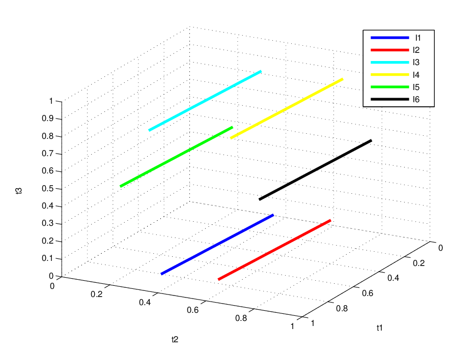
Furthermore, for the case N=3N=3 the points τ~k\widetilde{\tau}^{k} for k∈{1,2,…,6}k\in\{1,2,...,6\} lead to the set 𝒜3\mathcal{A}_{3} given by

𝒜3\displaystyle\mathcal{A}_{3} =ℓ1∪ℓ2∪ℓ3∪ℓ4∪ℓ5∪ℓ6\displaystyle=\ell_{1}\cup\ell_{2}\cup\ell_{3}\cup\ell_{4}\cup\ell_{5}\cup\ell_{6}
={τ:τ=[τ¯(ε+2)​τ¯e2+3​ε+3τ¯e2+3​ε+3]+𝟏s∈P3,s∈ℝ}∪{τ:τ=[τ¯τ¯e2+3​ε+3(ε+2)​τ¯e2+3​ε+3]+𝟏s∈P3,s∈ℝ}\displaystyle=\left\{\tau:\tau=\left[\begin{array}[]{c}\bar{\tau}\\ \frac{(\varepsilon+2)\bar{\tau}}{e^{2}+3\varepsilon+3}\\ \frac{\bar{\tau}}{e^{2}+3\varepsilon+3}\end{array}\right]+\mathbf{1}s\in P_{3},s\in\mathbb{R}\right\}\cup\left\{\tau:\tau=\left[\begin{array}[]{c}\bar{\tau}\\ \frac{\bar{\tau}}{e^{2}+3\varepsilon+3}\\ \frac{(\varepsilon+2)\bar{\tau}}{e^{2}+3\varepsilon+3}\end{array}\right]+\mathbf{1}s\in P_{3},s\in\mathbb{R}\right\}
∪{τ:τ=[(ε+2)​τ¯e2+3​ε+3τ¯τ¯e2+3​ε+3]+𝟏s∈P3,s∈ℝ}∪{τ:τ=[τ¯e2+3​ε+3τ¯(ε+2)​τ¯e2+3​ε+3]+𝟏s∈P3,s∈ℝ}\displaystyle\quad\cup\left\{\tau:\tau=\left[\begin{array}[]{c}\frac{(\varepsilon+2)\bar{\tau}}{e^{2}+3\varepsilon+3}\\ \bar{\tau}\\ \frac{\bar{\tau}}{e^{2}+3\varepsilon+3}\end{array}\right]+\mathbf{1}s\in P_{3},s\in\mathbb{R}\right\}\cup\left\{\tau:\tau=\left[\begin{array}[]{c}\frac{\bar{\tau}}{e^{2}+3\varepsilon+3}\\ \bar{\tau}\\ \frac{(\varepsilon+2)\bar{\tau}}{e^{2}+3\varepsilon+3}\end{array}\right]+\mathbf{1}s\in P_{3},s\in\mathbb{R}\right\}
∪{τ:τ=[(ε+2)​τ¯e2+3​ε+3τ¯e2+3​ε+3τ¯]+𝟏s∈P3,s∈ℝ}∪{τ:τ=[τ¯e2+3​ε+3(ε+2)​τ¯e2+3​ε+3τ¯]+𝟏s∈P3,s∈ℝ}\displaystyle\quad\cup\left\{\tau:\tau=\left[\begin{array}[]{c}\frac{(\varepsilon+2)\bar{\tau}}{e^{2}+3\varepsilon+3}\\ \frac{\bar{\tau}}{e^{2}+3\varepsilon+3}\\ \bar{\tau}\end{array}\right]+\mathbf{1}s\in P_{3},s\in\mathbb{R}\right\}\cup\left\{\tau:\tau=\left[\begin{array}[]{c}\frac{\bar{\tau}}{e^{2}+3\varepsilon+3}\\ \frac{(\varepsilon+2)\bar{\tau}}{e^{2}+3\varepsilon+3}\\ \bar{\tau}\end{array}\right]+\mathbf{1}s\in P_{3},s\in\mathbb{R}\right\}

Figure 4(a) shows these sets in the (τ1,τ2,τ3)(\tau_{1},\tau_{2},\tau_{3})-plane (solid colored). Figure 4(b) shows two solutions to ℋ3{\mathcal{H}}_{3}. Note how each simulation has jumps that take the trajectory close to different lines. This is due to a preservation of order for each τi\tau_{i} as seen in Lemma 2.7. This preservation of order will be used in the Lyapunov stability proof in the next section.

Refer to caption
(a) The desynchronization set 𝒜\mathcal{A} for N=3N=3, with τ¯=1\bar{\tau}=1 and ε=−0.3\varepsilon=-0.3.
Refer to caption
(b) Two solutions (magenta and cyan) to ℋ3{\mathcal{H}}_{3} such that τ⁡(0,0)∉𝒳3\tau(0,0)\notin\mathcal{X}_{3} with ε=−0.3\varepsilon=-0.3 and τ¯=1\bar{\tau}=1 showing the attractivity to 𝒜3=∪i=13!ℓi\mathcal{A}_{3}=\cup_{i=1}^{3!}\ell_{i}
Figure 4: 4(a) Set of points (ℓ1,ℓ2,…,ℓ6)(\ell_{1},\ell_{2},...,\ell_{6}) defining 𝒜3\mathcal{A}_{3} and 4(b) two simulations (dashed, one in cyan and the other in magenta) converging to the set 𝒜3\mathcal{A}_{3} (solid colored).

3.2 Lyapunov Stability

Lyapunov theory for hybrid systems is employed to show that the set of points 𝒜\mathcal{A} is asymptotically stable. Our candidate Lyapunov-like function, which is defined below and uses the distance function, is built by observing that there exist points where the distance to 𝒜\mathcal{A} may increase during flows. This is due to the sets ℓk\ell_{k} being a subset PNP_{N}. To avoid this issue, we define

𝒜~=⋃k=1N!ℓ~k⊃𝒜\widetilde{\mathcal{A}}=\bigcup_{k=1}^{N!}\widetilde{\ell}_{k}\supset\mathcal{A}

where ℓ~k\widetilde{\ell}_{k} is the extension of ℓk\ell_{k} given by

ℓ~k={τ∈ℝN:τ=τ~k+𝟏s,s∈ℝ}.\displaystyle\widetilde{\ell}_{k}=\left\{\tau\in\mathbb{R}^{N}:\tau=\widetilde{\tau}^{k}+\mathbf{1}s,s\in\mathbb{R}\right\}. (17)

Then, with this extended version of 𝒜\mathcal{A}, the proposed candidate Lyapunov-like function for asymptotic stability of 𝒜\mathcal{A} for ℋN{\mathcal{H}}_{N} is given by the locally Lipschitz function

V⁡(τ)=min⁡{|τ|ℓ~1,|τ|ℓ~2,…,|τ|ℓ~k,…,|τ|ℓ~N!}∀τ∈PN∖𝒳V(\tau)=\min\{|\tau|_{\widetilde{\ell}_{1}},|\tau|_{\widetilde{\ell}_{2}},\ldots,|\tau|_{\widetilde{\ell}_{k}},\ldots,|\tau|_{\widetilde{\ell}_{N}!}\}\quad\forall\ \tau\in P_{N}\setminus\mathcal{X} (18)

where, for some kk, |τ|ℓ~k|\tau|_{\widetilde{\ell}_{k}} is the distance between the point τ\tau and the set ℓ~k\widetilde{\ell}_{k}.55 5 The set ℓ~k\widetilde{\ell}_{k} can be described as a straight line in ℝn\mathbb{R}^{n} passing through a point τ~k\widetilde{\tau}^{k} and with slope 𝟏\mathbf{1}. Then, |τ|ℓ~k|\tau|_{\widetilde{\ell}_{k}} can be written as the general point-to-line distance |(τ~k−τ)−1/N⁡((τ~k−τ)⊤​𝟏)​𝟏||(\widetilde{\tau}^{k}-\tau)-1/N((\widetilde{\tau}^{k}-\tau)^{\top}\mathbf{1})\mathbf{1}|. The following theorem establishes asymptotic stability of 𝒜\mathcal{A} for ℋN{\mathcal{H}}_{N}. We show that the change in VV during flows is zero and that at jumps we have a strict decrease of VV; namely, V⁡(G⁡(τ))−V⁡(τ)=−|ε|​V​(τ)V(G(\tau))-V(\tau)=-|\varepsilon|V(\tau). A key step in the proof is in using [16, Theorem 8.2] on a restricted version of ℋN{\mathcal{H}}_{N}.

Theorem 3.3

For every N∈ℕ,N>1N\in\mathbb{N},N>1, τ¯>0,ω>0\bar{\tau}>0,\omega>0, and ε∈(−1,0)\varepsilon\in(-1,0), the hybrid system ℋN{\mathcal{H}}_{N} is such that the compact set 𝒜\mathcal{A} is

  1. 1.

    asymptotically stable with basin of attraction given by ℬ𝒜:=PN∖𝒳\mathcal{B}_{\mathcal{A}}:=P_{N}\setminus\mathcal{X}.

  2. 2.

    weakly globally asymptotically stable.

Let the set 𝒳v\mathcal{X}_{v} define the vv-inflation of 𝒳\mathcal{X} (defined in Lemma 2.6), that is, the open set66 6 The set 𝒳v\mathcal{X}_{v} is open since every point τ∈𝒳v\tau\in\mathcal{X}_{v} is an interior point of 𝒳v\mathcal{X}_{v}. 𝒳v:={τ∈ℝN:|τ|𝒳<v}\mathcal{X}_{v}:=\{\tau\in\mathbb{R}^{N}:|\tau|_{\mathcal{X}}<v\}, where v∈(0,v∗)v\in(0,v^{*}) and v∗=minx∈𝒳,y∈𝒜~⁡|x−y|v^{*}=\min_{x\in\mathcal{X},y\in\widetilde{\mathcal{A}}}|x-y|. Given any v∈(0,v∗)v\in(0,v^{*}), we now consider a restricted hybrid system ℋ~N=(f,C~,G,D~)\widetilde{\mathcal{H}}_{N}=(f,\widetilde{C},G,\widetilde{D}), where C~:=C∖𝒳v\widetilde{C}:=C\setminus\mathcal{X}_{v} and D~:=D∖𝒳v\widetilde{D}:=D\setminus\mathcal{X}_{v}, which are closed. We establish that 𝒜~\widetilde{\mathcal{A}} is an asymptotically stable set for ℋ~N\widetilde{\mathcal{H}}_{N}.

Note that the continuous function VV, given by (18), is defined as the minimum distance from τ\tau to 𝒜~\widetilde{\mathcal{A}}, where 𝒜~\widetilde{\mathcal{A}} is the union of N!N! sets ℓ~k\widetilde{\ell}_{k} in (17). To determine the change of VV during flows77 7 Its derivative can be computed using Clarke’s generalized gradient [19]., we consider the relationship between the flow map and the sets ℓ~k\widetilde{\ell}_{k}. The inner product between a vector pointing in the direction of the set ℓ~k\widetilde{\ell}_{k} and the flow map on C~\widetilde{C} satisfies

𝟏⊤​f​(τ)=𝟏⊤​(ω​𝟏)=ω​N=|𝟏|​|ω​𝟏|=|𝟏||f⁡(τ)|cos⁡θ\mathbf{1}^{\top}f(\tau)=\mathbf{1}^{\top}(\omega\mathbf{1})=\omega N=|\mathbf{1}||\omega\mathbf{1}|=|\mathbf{1}||f(\tau)|\cos\theta

, which is only true if θ\theta is zero. Therefore, the direction of the flow map and of the vector defining ℓ~k\widetilde{\ell}_{k} are parallel, implying that the distance to the set 𝒜~\widetilde{\mathcal{A}} is constant during flows.

The change in VV during jumps is given by V⁡(G⁡(τ))−V⁡(τ)V(G(\tau))-V(\tau) for τ∈D~∖𝒜~\tau\in\widetilde{D}\setminus\widetilde{\mathcal{A}}. Due to the fact that we can rearrange the components of τ∈PN∖𝒳\tau\in P_{N}\setminus\mathcal{X}, without loss of generality, we consider a single jump condition, namely, we consider τ\tau such that τ¯=τ1>τ2>…>τN−1>τN\bar{\tau}=\tau_{1}>\tau_{2}>\ldots>\tau_{N-1}>\tau_{N}. Using the formulation in Section 3.1 and Lemma A.1, the elements of the vector τ~k\widetilde{\tau}^{k} associated with ℓ~k\widetilde{\ell}_{k} for this case of τ\tau are given by τ~ik=∑p=0N−i(ε+1)p∑p=0N−1(ε+1)p​τ¯\widetilde{\tau}_{i}^{k}=\frac{\sum_{p=0}^{N-i}(\varepsilon+1)^{p}}{\sum_{p=0}^{N-1}(\varepsilon+1)^{p}}\bar{\tau}, which by Lemma A.2 is equal to (ε+1)N−i+1−1(ε+1)N−1​τ¯\frac{(\varepsilon+1)^{N-i+1}-1}{(\varepsilon+1)^{N}-1}\bar{\tau}. After the jump, G⁡(τ)G(\tau) is single valued and is such that its elements are ordered as follows: g2​(τ)>g3​(τ)>…>gN​(τ)>g1​(τ)=0.g_{2}(\tau)>g_{3}(\tau)>\ldots>g_{N}(\tau)>g_{1}(\tau)=0. Specifically, the jump map is G⁡(τ)=[0,(1+ε)​τ2,…,(1+ε)​τN]⊤G(\tau)=[0,(1+\varepsilon)\tau_{2},\ldots,(1+\varepsilon)\tau_{N}]^{\top}. Then, the formulation in Section 3.1 and Lemma A.1 leads to a case of τ~k\widetilde{\tau}^{k} denoted as τ~k′\widetilde{\tau}^{k^{\prime}}. By Lemma A.2, the elements of the vector τ~k′\widetilde{\tau}^{k^{\prime}} are given by τ~1k′=ε(ε+1)N−1​τ¯\widetilde{\tau}^{k^{\prime}}_{1}=\frac{\varepsilon}{(\varepsilon+1)^{N}-1}\bar{\tau} and τ~ik′=(ε+1)N−i+2−1(ε+1)N−1​τ¯\widetilde{\tau}^{k^{\prime}}_{i}=\frac{(\varepsilon+1)^{N-i+2}-1}{(\varepsilon+1)^{N}-1}\bar{\tau} for i>1i>1. Due to the ordering of τ\tau and G⁡(τ)G(\tau), τ~k′\widetilde{\tau}^{k^{\prime}} is a one-element shifted (to the right) version of τ~k\widetilde{\tau}^{k}.

From the definition of τ~k\widetilde{\tau}^{k} above, VV at τ\tau reduces to

V⁡(τ)=|τ|ℓ~k=|(τ~k−τ)−1N​((τ~k−τ)⊤​𝟏)​𝟏|V(\tau)=|\tau|_{\widetilde{\ell}_{k}}=\left|(\widetilde{\tau}^{k}-\tau)-\frac{1}{N}((\widetilde{\tau}^{k}-\tau)^{\top}\mathbf{1})\mathbf{1}\right|

for some kk. Note that

(τ~k−τ)⊤​𝟏=∑i=1Nτ~ik−∑i=1Nτi(\widetilde{\tau}^{k}-\tau)^{\top}\mathbf{1}=\sum_{i=1}^{N}\widetilde{\tau}^{k}_{i}-\sum_{i=1}^{N}\tau_{i}

reduces to ∑i=2Nτ~ik−∑i=2Nτi\sum_{i=2}^{N}\widetilde{\tau}^{k}_{i}-\sum_{i=2}^{N}\tau_{i} since τ1=τ~1k=τ¯\tau_{1}=\widetilde{\tau}_{1}^{k}=\bar{\tau}. Using Lemmas A.2 and A.3, it follows that

∑i=2Nτ~ik=∑i=2N∑p=0N−i(ε+1)p∑p=0N−1(ε+1)p​τ¯=((ε+1)N−1)−N​εε⁡((ε+1)N−1)​τ¯.\sum_{i=2}^{N}\widetilde{\tau}^{k}_{i}=\frac{\sum_{i=2}^{N}\sum_{p=0}^{N-i}(\varepsilon+1)^{p}}{\sum_{p=0}^{N-1}(\varepsilon+1)^{p}}\bar{\tau}=\frac{((\varepsilon+1)^{N}-1)-N\varepsilon}{\varepsilon((\varepsilon+1)^{N}-1)}\bar{\tau}.

Then, the first element of the vector inside the norm in the expression of V⁡(τ)V(\tau) is given as

(τ~1k−τ1)−1N​(((ε+1)N−1)−N​εε⁡((ε+1)N−1)​τ¯−∑i=2Nτi)\displaystyle(\widetilde{\tau}^{k}_{1}-\tau_{1})-\frac{1}{N}\left(\frac{((\varepsilon+1)^{N}-1)-N\varepsilon}{\varepsilon((\varepsilon+1)^{N}-1)}\bar{\tau}-\sum_{i=2}^{N}\tau_{i}\right)
=−((ε+1)N−1)−N​εε​N​((ε+1)N−1)​τ¯+1N​∑i=2Nτi,\displaystyle\qquad\qquad\qquad\qquad=-\frac{((\varepsilon+1)^{N}-1)-N\varepsilon}{\varepsilon N((\varepsilon+1)^{N}-1)}\bar{\tau}+\frac{1}{N}\sum_{i=2}^{N}\tau_{i},

while the elements with m∈{2,3,…,N}m\in\{2,3,\ldots,N\} are given by

(τ~mk−τm)−1N​(((ε+1)N−1)−N​εε⁡((ε+1)N−1)​τ¯−∑i=2Nτi)\displaystyle(\widetilde{\tau}_{m}^{k}-\tau_{m})-\frac{1}{N}\left(\frac{((\varepsilon+1)^{N}-1)-N\varepsilon}{\varepsilon((\varepsilon+1)^{N}-1)}\bar{\tau}-\sum_{i=2}^{N}\tau_{i}\right) =\displaystyle= ((ε+1)N−m+1−1(ε+1)N−1​τ¯−τm)−\displaystyle\left(\frac{(\varepsilon+1)^{N-m+1}-1}{(\varepsilon+1)^{N}-1}\bar{\tau}-\tau_{m}\right)-
1N​(((ε+1)N−1)−N​εε⁡((ε+1)N−1)​τ¯−∑i=2Nτi)\displaystyle\qquad\qquad\qquad\qquad\frac{1}{N}\left(\frac{((\varepsilon+1)^{N}-1)-N\varepsilon}{\varepsilon((\varepsilon+1)^{N}-1)}\bar{\tau}-\sum_{i=2}^{N}\tau_{i}\right)
=\displaystyle= ε​N​(ε+1)N−m+1−((ε+1)N−1)ε​N​((ε+1)N−1)​τ¯\displaystyle\frac{\varepsilon N(\varepsilon+1)^{N-m+1}-((\varepsilon+1)^{N}-1)}{\varepsilon N((\varepsilon+1)^{N}-1)}\bar{\tau}
−N−1N​τm+1N​∑i=2,i≠mNτi.\displaystyle\qquad\qquad\qquad\qquad\qquad\qquad-\frac{N-1}{N}\tau_{m}+\frac{1}{N}\sum_{i=2,i\neq m}^{N}\tau_{i}.

After the jump at τ\tau, since G⁡(τ)G(\tau) is single valued, V⁡(G⁡(τ))V(G(\tau)) is given by

|G⁡(τ)|ℓ~k′=|(τ~k′−G⁡(τ))−1N​((τ~k′−G⁡(τ))⊤​𝟏)​𝟏|.|G(\tau)|_{\widetilde{\ell}_{k^{\prime}}}=\left|(\widetilde{\tau}^{k^{\prime}}-G(\tau))-\frac{1}{N}((\widetilde{\tau}^{k^{\prime}}-G(\tau))^{\top}\mathbf{1})\mathbf{1}\right|.

Note that (τ~k′−G⁡(τ))⊤​𝟏=∑i=1Nτ~ik′−∑i=1Ngi​(τ)(\widetilde{\tau}^{k^{\prime}}-G(\tau))^{\top}\mathbf{1}=\sum_{i=1}^{N}\widetilde{\tau}^{k^{\prime}}_{i}-\sum_{i=1}^{N}g_{i}(\tau) reduces to ∑i=1Nτ~ik′−∑i=2N(1+ε)​τi\sum_{i=1}^{N}\widetilde{\tau}^{k^{\prime}}_{i}-\sum_{i=2}^{N}(1+\varepsilon)\tau_{i}, since g1​(τ)=0g_{1}(\tau)=0 and gi​(τ)=(1+ε)​τig_{i}(\tau)=(1+\varepsilon)\tau_{i} for i>1i>1. Using Lemmas A.2 and A.3, it follows that

∑i=1Nτ~ik′\displaystyle\sum_{i=1}^{N}\widetilde{\tau}^{k^{\prime}}_{i} =∑i=1N∑p=0N−i(ε+1)p∑p=0N−1(ε+1)p​τ¯\displaystyle=\frac{\sum_{i=1}^{N}\sum_{p=0}^{N-i}(\varepsilon+1)^{p}}{\sum_{p=0}^{N-1}(\varepsilon+1)^{p}}\bar{\tau}
=(ε+1)​((ε+1)N−1)−N​εε⁡((ε+1)N−1)​τ¯\displaystyle=\frac{(\varepsilon+1)((\varepsilon+1)^{N}-1)-N\varepsilon}{\varepsilon((\varepsilon+1)^{N}-1)}\bar{\tau}

which leads to

(τ~k′−G⁡(τ))⊤​𝟏=(ε+1)​((ε+1)N−1)−N​εε⁡((ε+1)N−1)​τ¯−∑i=2N(1+ε)​τi.(\widetilde{\tau}^{k^{\prime}}-G(\tau))^{\top}\mathbf{1}=\frac{(\varepsilon+1)((\varepsilon+1)^{N}-1)-N\varepsilon}{\varepsilon((\varepsilon+1)^{N}-1)}\bar{\tau}-\sum_{i=2}^{N}(1+\varepsilon)\tau_{i}.

The first element inside the norm in V⁡(G⁡(τ))V(G(\tau)) is given by

(τ~1k′−g1​(τ))−1N​((ε+1)​((ε+1)N−1)−N​εε⁡((ε+1)N−1)​τ¯CLOSE\displaystyle(\widetilde{\tau}_{1}^{k^{\prime}}-g_{1}(\tau))-\frac{1}{N}\left(\frac{(\varepsilon+1)((\varepsilon+1)^{N}-1)-N\varepsilon}{\varepsilon((\varepsilon+1)^{N}-1)}\bar{\tau}\right.
−∑i=2N(1+ε)τi)\displaystyle\qquad\qquad\qquad\qquad\qquad\qquad\qquad\qquad\qquad\left.-\sum_{i=2}^{N}(1+\varepsilon)\tau_{i}\right)
=ε(ε+1)N−1​τ¯−(ε+1)​((ε+1)N−1)−N​εε​N​((ε+1)N−1)​τ¯\displaystyle=\frac{\varepsilon}{(\varepsilon+1)^{N}-1}\bar{\tau}-\frac{(\varepsilon+1)((\varepsilon+1)^{N}-1)-N\varepsilon}{\varepsilon N((\varepsilon+1)^{N}-1)}\bar{\tau}
+1N∑i=2N(1+ε)τi\displaystyle\qquad\qquad\qquad\qquad\qquad\qquad\qquad\qquad\qquad+\frac{1}{N}\sum_{i=2}^{N}(1+\varepsilon)\tau_{i}
=(1+ε)​(−((ε+1)N−1)−N​εε​N​((ε+1)N−1)​τ¯+1N​∑i=2Nτi).\displaystyle=(1+\varepsilon)\left(-\frac{((\varepsilon+1)^{N}-1)-N\varepsilon}{\varepsilon N((\varepsilon+1)^{N}-1)}\bar{\tau}+\frac{1}{N}\sum_{i=2}^{N}\tau_{i}\right).

For each element m>1m>1, it follows that

(τ~mk′−gm​(τ))\displaystyle(\widetilde{\tau}^{k^{\prime}}_{m}-g_{m}(\tau)) −\displaystyle- 1N​((ε+1)​((ε+1)N−1)−N​εε⁡((ε+1)N−1)​τ¯−∑i=2N(1+ε)​τi)\displaystyle\frac{1}{N}\left(\frac{(\varepsilon+1)((\varepsilon+1)^{N}-1)-N\varepsilon}{\varepsilon((\varepsilon+1)^{N}-1)}\bar{\tau}-\sum_{i=2}^{N}(1+\varepsilon)\tau_{i}\right)
=\displaystyle= (ε+1)N−m+2−1(ε+1)N−1​τ¯−(1+ε)​N−1N​τm−(ε+1)​((ε+1)N−1)−N​εε​N​((ε+1)N−1)​τ¯+1N​∑i=2,i≠mN(1+ε)​τi\displaystyle\frac{(\varepsilon+1)^{N-m+2}-1}{(\varepsilon+1)^{N}-1}\bar{\tau}-(1+\varepsilon)\frac{N-1}{N}\tau_{m}-\frac{(\varepsilon+1)((\varepsilon+1)^{N}-1)-N\varepsilon}{\varepsilon N((\varepsilon+1)^{N}-1)}\bar{\tau}+\frac{1}{N}\sum_{i=2,i\neq m}^{N}(1+\varepsilon)\tau_{i}
=\displaystyle= (1+ε)​(ε​N​(ε+1)N−m+1−((ε+1)N−1)ε​N​((ε+1)N−1)​τ¯−N−1N​τm+1N​∑i=2,i≠mNτi).\displaystyle(1+\varepsilon)\left(\frac{\varepsilon N(\varepsilon+1)^{N-m+1}-((\varepsilon+1)^{N}-1)}{\varepsilon N((\varepsilon+1)^{N}-1)}\bar{\tau}-\frac{N-1}{N}\tau_{m}+\frac{1}{N}\sum_{i=2,i\neq m}^{N}\tau_{i}\right).

Combining the expressions for each of the elements inside the norm of V⁡(G⁡(τ))V(G(\tau)), it follows that V⁡(G⁡(τ))=(1+ε)​V​(τ)V(G(\tau))=(1+\varepsilon)V(\tau).

Then, the change during jumps is given by V⁡(G⁡(τ))−V⁡(τ)=ε​V​(τ)V(G(\tau))-V(\tau)=\varepsilon V(\tau) where ε∈(−1,0)\varepsilon\in(-1,0). With the property of VV during flows established above, the change of VV along solutions is bounded during flows and jumps by the nonpositive functions uC~u_{\widetilde{C}} and uD~u_{\widetilde{D}}, respectively, defined as follows: uC~​(z)=0u_{\widetilde{C}}(z)=0 for each z∈C~z\in\widetilde{C} and uC~​(z)=−∞u_{\widetilde{C}}(z)=-\infty otherwise; uD~​(z)=ε​V​(z)u_{\widetilde{D}}(z)=\varepsilon V(z) for each z∈D~z\in\widetilde{D} and uD~​(z)=−∞u_{\widetilde{D}}(z)=-\infty otherwise. Using Lemma 2.1, the fact that C~\widetilde{C} and D~\widetilde{D} are closed, and the fact that every maximal solution to ℋ~\widetilde{\mathcal{H}} is bounded and complete, by [16, Theorem 8.2], every maximal solution to ℋ~N\widetilde{\mathcal{H}}_{N} approaches the largest weakly invariant subset of LV​(r′)∩C~∩[LuC~​(0)∪(LuD~​(0)∩G⁡(LuC~​(0)))]=LV​(r′)∩C~L_{V}(r^{\prime})\cap\widetilde{C}\cap[L_{u_{\widetilde{C}}}(0)\cup(L_{u_{\widetilde{D}}}(0)\cap G(L_{u_{\widetilde{C}}}(0)))]=L_{V}(r^{\prime})\cap\widetilde{C} for r′∈V⁡(C~)r^{\prime}\in V(\widetilde{C}). Since every maximal solution jumps an infinite number of times, the largest invariant set is given for r′=0r^{\prime}=0 due to the fact that V⁡(G⁡(τ))−V⁡(τ)=ε​V​(τ)<0V(G(\tau))-V(\tau)=\varepsilon V(\tau)<0 if r′>0r^{\prime}>0. Then, the largest invariant set is given by LV​(0)∩C~=𝒜~∩C~L_{V}(0)\cap\widetilde{C}=\widetilde{\mathcal{A}}\cap\widetilde{C} which is identically equal to 𝒜\mathcal{A}. Hence, the set 𝒜\mathcal{A} is attractive. Stability is guaranteed from the fact that VV is nonincreasing during flows and strictly decreasing during jumps. Then, the set 𝒜~\widetilde{\mathcal{A}} is asymptotically stable for the hybrid system ℋ~N\widetilde{\mathcal{H}}_{N}. We have that 𝒜\mathcal{A} is (strongly) forward invariant and from Theorem 3.4 we know that 𝒜\mathcal{A} is uniformly attractive from a neighborhood of itself. Then by Proposition 7.5 in [16], it follows that 𝒜\mathcal{A} is asymptotically stable.

Note that the set of solutions to ℋ~N\widetilde{\mathcal{H}}_{N} coincides with the set of solutions to ℋN{\mathcal{H}}_{N} from PN∖𝒳vP_{N}\setminus\mathcal{X}_{v}. Therefore, the set 𝒜\mathcal{A} is asymptotically stable for ℋN{\mathcal{H}}_{N} with basin of attraction ℬ𝒜=PN∖𝒳v{\mathcal{B}}_{\mathcal{A}}=P_{N}\setminus\mathcal{X}_{v}. Since vv is arbitrary, it follows that the basin of attraction is equal to PN∖𝒳P_{N}\color[rgb]{0,0,0}\setminus\mathcal{X}.

Note that the jump map GG, at points τ∈𝒳\tau\in\mathcal{X}, is set valued by definition of gig_{i} in (4). From these points there exist solutions to ℋN{\mathcal{H}}_{N} that jump out of 𝒳\mathcal{X}. In fact, consider the case τ∈𝒳\tau\in\mathcal{X}. We have that τi=τr\tau_{i}=\tau_{r} for some i,r∈Ii,r\in I. Then, after the jump it follows that gi​(τ)∈{0,(1+ε)​τ¯}g_{i}(\tau)\in\{0,(1+\varepsilon)\bar{\tau}\} and gr​(τ)∈{0,(1+ε)​τ¯},g_{r}(\tau)\in\{0,(1+\varepsilon)\bar{\tau}\}, and there exist gig_{i} and grg_{r} such that gi=grg_{i}=g_{r} or gi≠grg_{i}\neq g_{r}. Since for every point in 𝒳\mathcal{X} there exists a solution that converges to 𝒜\mathcal{A} and also a solution that stays in 𝒳\mathcal{X}, 𝒳\mathcal{X} is weakly forward invariant.88 8 For example, consider the case N=2N=2. If τ⁡(0,0)=[τ¯,τ¯]⊤∈D\tau(0,0)=[\bar{\tau},\bar{\tau}]^{\top}\in D, then there are nonunique solutions due to the jump map begin set valued. It follows that after the jump, each τi\tau_{i} can be mapped to any point in {0,τi​(1+ε)}\{0,\tau_{i}(1+\varepsilon)\}, which leads to any of the following four options of the states (τ1,τ2)(\tau_{1},\tau_{2}) after such a jump: (0,0),(0,τ¯​(1+ε)),(τ¯​(1+ε),0)(0,0),(0,\bar{\tau}(1+\varepsilon)),(\bar{\tau}(1+\varepsilon),0) or (τ¯​(1+ε),τ¯​(1+ε))(\bar{\tau}(1+\varepsilon),\bar{\tau}(1+\varepsilon)). If the state is mapped to either (0,0)(0,0) or (τ¯​(1+ε),τ¯​(1+ε))(\bar{\tau}(1+\varepsilon),\bar{\tau}(1+\varepsilon)), then it remains in 𝒳2\mathcal{X}_{2}. Conversely, if any of the other options are chosen, then (τ1,τ2)(\tau_{1},\tau_{2}) leaves 𝒳2\mathcal{X}_{2} and converges to 𝒜\mathcal{A} asymptotically.

3.3 Characterization of Time of Convergence

In this section, we characterize the time to converge to a neighborhood of 𝒜\mathcal{A}. The proposed (upper bound) of the time to converge depends on the initial distance to the set 𝒜~\widetilde{\mathcal{A}} and the parameters of the hybrid system (ε,τ¯)(\varepsilon,\bar{\tau}).

Theorem 3.4

For every N∈ℕN\in\mathbb{N}, N>1N>1, and every c1,c2c_{1},c_{2} such that c¯>c2>c1>0\overline{c}>c_{2}>c_{1}>0 with c¯=maxx∈𝒳⁡|x|𝒜~\overline{c}=\max_{x\in\mathcal{X}}|x|_{\widetilde{\mathcal{A}}}, every maximal solution to ℋN{\mathcal{H}}_{N} with initial condition τ⁡(0,0)∈(PN∖𝒳)∩L~V​(c2)\tau(0,0)\in(P_{N}\setminus\mathcal{X})\cap\widetilde{L}_{V}(c_{2}) is such that

τ⁡(t,j)∈L~V​(c1)∀(t,j)∈domτ,t+j≥M,\tau(t,j)\in\widetilde{L}_{V}(c_{1})\ \ \forall(t,j)\in\mathop{\rm dom}\nolimits\tau,t+j\geq M,

where

M=(τ¯ω+1)​log⁡c2c1log⁡11+εM=\left(\frac{\bar{\tau}}{\omega}+1\right)\frac{\log\frac{c_{2}}{c_{1}}}{\log\frac{1}{1+\varepsilon}}

and L~V​(μ):={τ∈C∪D:V⁡(τ)≤μ}\widetilde{L}_{V}(\mu):=\{\tau\in C\cup D:V(\tau)\leq\mu\}.

Refer to caption
Figure 5: Time to converge (over τ¯+1\bar{\tau}+1) as a function of ε∈[−0.9,−0.1]\varepsilon\in[-0.9,-0.1], with c2=0.99​τ¯c_{2}=0.99\bar{\tau} and c1∈{0.5​τ¯,0.3​τ¯,0.1​τ¯,0.05​τ¯}c_{1}\in\{0.5\bar{\tau},0.3\bar{\tau},0.1\bar{\tau},0.05\bar{\tau}\}

Let τ0=τ⁡(0,0)\tau_{0}=\tau(0,0) and pick a maximal solution τ\tau to ℋN{\mathcal{H}}_{N} from τ0\tau_{0}. At every jump time (tj,j)∈domτ(t_{j},j)\in\mathop{\rm dom}\nolimits\tau, define g¯1=τ⁡(t1,1)\bar{g}_{1}=\tau(t_{1},1), g¯2=τ⁡(t2,2),…,g¯J=τ⁡(tJ,J)\bar{g}_{2}=\tau(t_{2},2),\ldots,\bar{g}_{J}=\tau(t_{J},J), for some J∈ℕJ\in\mathbb{N}. From Theorem 3.3, we have that there is no change in the Lyapunov function during flows. Furthermore, we have that for each τ∈D∖𝒜\tau\in D\setminus\mathcal{A} the difference V⁡(G⁡(τ))−V⁡(τ)=ε​V​(τ)V(G(\tau))-V(\tau)=\varepsilon V(\tau) with ε∈(−1,0)\varepsilon\in(-1,0). Since, for every j,j, τ⁡(tj,j)∈D\tau(t_{j},j)\in D, we have

V⁡(g¯1)−V⁡(τ0)=ε​V​(τ0),V(\bar{g}_{1})-V(\tau_{0})=\varepsilon V(\tau_{0}),

which implies

V⁡(g¯1)=(1+ε)​V​(τ0).V(\bar{g}_{1})=(1+\varepsilon)V(\tau_{0}).

At the next jump, we have

V⁡(g¯2)=(1+ε)​V​(g¯1)=(1+ε)2​V​(τ0).V(\bar{g}_{2})=(1+\varepsilon)V(\bar{g}_{1})=(1+\varepsilon)^{2}V(\tau_{0}).

Proceeding in this way, after JJ jumps we have

V⁡(g¯J)=(1+ε)​V​(gJ−1)=(1+ε)J​V​(τ0).V(\bar{g}_{J})=(1+\varepsilon)V(g_{J-1})=(1+\varepsilon)^{J}V(\tau_{0}).

From V⁡(g¯J)=(1+ε)J​V​(τ0)V(\bar{g}_{J})=(1+\varepsilon)^{J}V(\tau_{0}), we want to find JJ so that V⁡(g¯J)≤c1V(\bar{g}_{J})\leq c_{1} when V⁡(τ0)≤c2V(\tau_{0})\leq c_{2}. Considering the worst cast for V⁡(τ0)V(\tau_{0}), we want (1+ε)J​c2≤c1(1+\varepsilon)^{J}c_{2}\leq c_{1}, which implies c2c1≤(11+ε)J\frac{c_{2}}{c_{1}}\leq\left(\frac{1}{1+\varepsilon}\right)^{J}, and therefore J=⌈log⁡c2c1log⁡11+ε⌉>0.J=\left\lceil\frac{\log\frac{c_{2}}{c_{1}}}{\log\frac{1}{1+\varepsilon}}\right\rceil>0. For each jj, the time between jumps satisfies t1−t0≤τ¯ω,t2−t1≤τ¯ω,…,tj−tj−1≤τ¯ω.t_{1}-t_{0}\leq\frac{\bar{\tau}}{\omega},t_{2}-t_{1}\leq\frac{\bar{\tau}}{\omega},\ldots,t_{j}-t_{j-1}\leq\frac{\bar{\tau}}{\omega}. Then, we have that after JJ jumps, ∑j=1Jtj−tj−1≤J​τ¯ω.\sum_{j=1}^{J}t_{j}-t_{j-1}\leq J\frac{\bar{\tau}}{\omega}. With t0=0t_{0}=0, the expression reduces to tJ≤J​τ¯ω=⌈log⁡c2c1log⁡11+ε⌉​τ¯ω.t_{J}\leq J\frac{\bar{\tau}}{\omega}=\left\lceil\frac{\log\frac{c_{2}}{c_{1}}}{\log\frac{1}{1+\varepsilon}}\right\rceil\frac{\bar{\tau}}{\omega}. Then, after t+j≥tJ+Jt+j\geq t_{J}+J, the solution is at least c1c_{1} close to the set 𝒜~\widetilde{\mathcal{A}}. Defining M=tJ+JM=t_{J}+J we then have

M=(τ¯ω+1)​⌈log⁡c2c1log⁡11+ε⌉.M=\left(\frac{\bar{\tau}}{\omega}+1\right)\left\lceil\frac{\log\frac{c_{2}}{c_{1}}}{\log\frac{1}{1+\varepsilon}}\right\rceil.

Figure 5 shows the time to converge (divided by τ¯ω+1\frac{\bar{\tau}}{\omega}+1) versus ε\varepsilon with constant c2=0.99​τ¯c_{2}=0.99\bar{\tau} and varying values of c1c_{1}. As the figure indicates, the time to converge decreases as |ε||\varepsilon| increases, which confirms the intuition that the larger the jump the faster oscillators desynchronize.

3.4 Robustness Analysis

Lemma 2.1 establishes that the hybrid model of NN impulse-coupled oscillators satisfies the hybrid basic conditions. In light of this property, the asymptotic stability property of 𝒜\mathcal{A} for ℋN{\mathcal{H}}_{N} is preserved under certain perturbations; i.e., asymptotic stability is robust [16]. In the next sections, we consider a perturbed version of ℋN{\mathcal{H}}_{N} and present robust stability results. In particular, we consider generic perturbations to ℋN{\mathcal{H}}_{N}, and two different cases of perturbations only on the timer rates to allow for heterogeneous timers.

3.4.1 Robustness to Generic Perturbations

We start by revisiting the definition of perturbed hybrid systems in [16].

Definition 3.5 (perturbed hybrid system [16, Definition 6.27])

Given a hybrid system ℋ{\mathcal{H}} and a function ρ:ℝN→ℝ≥0\rho:\mathbb{R}^{N}\to\mathbb{R}_{\geq 0}, the ρ\rho-perturbation of ℋ{\mathcal{H}}, denoted ℋρ{\mathcal{H}}_{\rho}, is the hybrid system

{x∈Cρx˙∈Fρ​(x)x∈Dρx+∈Gρ​(x)\left\{\begin{array}[]{cc}x\in C_{\rho}&\quad\dot{x}\in F_{\rho}(x)\\ x\in D_{\rho}&\quad x^{+}\in G_{\rho}(x)\\ \end{array}\right.

where

Cρ\displaystyle C_{\rho} ={x∈ℝn:(x+ρ⁡(x)​𝔹)∩C≠∅},\displaystyle=\{x\in\mathbb{R}^{n}:(x+\rho(x)\mathbb{B})\cap C\neq\emptyset\},
Fρ​(x)\displaystyle F_{\rho}(x) =con¯​F​((x+ρ⁡(x)​𝔹)∩C)+ρ⁡(x)​𝔹∀x∈ℝn,\displaystyle=\overline{\mathrm{con}}F((x+\rho(x)\mathbb{B})\cap C)+\rho(x)\mathbb{B}\quad\forall x\in\mathbb{R}^{n},
Dρ\displaystyle D_{\rho} ={x∈ℝn:(x+ρ⁡(x)​𝔹)∩D≠∅},\displaystyle=\{x\in\mathbb{R}^{n}:(x+\rho(x)\mathbb{B})\cap D\neq\emptyset\},
Gρ​(x)\displaystyle G_{\rho}(x) ={v∈ℝn:v∈g+ρ(g)𝔹,g∈G((x+ρ(x)𝔹)∩D)}∀x∈ℝn.\displaystyle=\{v\in\mathbb{R}^{n}:v\in g+\rho(g)\mathbb{B},g\in G((x+\rho(x)\mathbb{B})\cap D)\}\quad\forall x\in\mathbb{R}^{n}.

Using this definition, we can deduce a generic perturbed hybrid system modeling NN impulse-coupled oscillators. Then, for the hybrid system ℋN{\mathcal{H}}_{N}, we denote ℋN,ρ{\mathcal{H}}_{N,\rho} as the ρ\rho-perturbation of ℋN{\mathcal{H}}_{N}. Given the perturbation function ρ:ℝN→ℝ≥0\rho:\mathbb{R}^{N}\to\mathbb{R}_{\geq 0}, the perturbed flow map is given by

Fρ​(τ)\displaystyle F_{\rho}(\tau) =ω​𝟏+ρ⁡(τ)​𝔹∀τ∈Cρ,\displaystyle=\omega\mathbf{1}+\rho(\tau)\mathbb{B}\qquad\forall\ \tau\in C_{\rho},

where the perturbed flow set CρC_{\rho} is given by

Cρ\displaystyle C_{\rho} ={τ∈ℝN:(τ+ρ⁡(τ)​𝔹)∩PN≠∅}.\displaystyle=\{\tau\in\mathbb{R}^{N}:(\tau+\rho(\tau)\mathbb{B})\cap P_{N}\neq\emptyset\}.

For example, if N=2N=2 and ρ⁡(τ)=ρ¯>0\rho(\tau)=\bar{\rho}>0 for all τ∈ℝN\tau\in\mathbb{R}^{N}, which would correspond to constant perturbations on the lower value and threshold, then Cρ=C+ρ​𝔹C_{\rho}=C+\rho\mathbb{B}. The perturbed jump map and jump set are defined as

Dρ\displaystyle D_{\rho} ={τ∈ℝN:(τ+ρ⁡(τ)​𝔹)∩D≠∅},\displaystyle=\{\tau\in\mathbb{R}^{N}:(\tau+\rho(\tau)\mathbb{B})\cap D\neq\emptyset\},
Gρ\displaystyle G_{\rho} =[g1,ρ​(τ),…,gN,ρ​(τ)]⊤,\displaystyle=[g_{1,\rho}(\tau),\ldots,g_{N,\rho}(\tau)]^{\top},

where gi,ρg_{i,\rho} is the ii-th component of GρG_{\rho}. The following result establishes that the hybrid system ℋN{\mathcal{H}}_{N} is robust to small perturbations.

Theorem 3.6

(robustness of asymptotic stability) If ρ:ℝN→ℝ≥0\rho:\mathbb{R}^{N}\to\mathbb{R}_{\geq 0} is continuous and positive on ℝN∖𝒜\mathbb{R}^{N}\setminus\mathcal{A}, then 𝒜\mathcal{A} is semiglobally practically robustly 𝒦​ℒ\mathcal{KL} asymptotically stable with basin of attraction B𝒜=PN∖𝒳B_{\mathcal{A}}=P_{N}\setminus\mathcal{X}, i.e., for every compact set K⊂B𝒜K\subset B_{\mathcal{A}} and every α>0\alpha>0, there exists δ∈(0,1)\delta\in(0,1) such that every maximal solution τ\tau to ℋN,δ​ρ{\mathcal{H}}_{N,\delta\rho} from KK satisfies |τ⁡(t,j)|𝒜≤β⁡(|τ⁡(0,0)|𝒜,t+j)+α|\tau(t,j)|_{\mathcal{A}}\leq\beta(|\tau(0,0)|_{\mathcal{A}},t+j)+\alpha for all (t,j)∈domτ(t,j)\in\mathop{\rm dom}\nolimits\tau.

From Lemma 2.1, the hybrid system ℋN{\mathcal{H}}_{N} satisfies the hybrid basic conditions. Therefore, by [16, Theorem 6.8] ℋN{\mathcal{H}}_{N} is nominally well-posed and, moreover, by [16, Proposition 6.28] is well-posed. From the proof of Theorem 3.3, we know that the set 𝒜\mathcal{A} is an asymptotically stable compact set for the hybrid system ℋN{\mathcal{H}}_{N} with basin of attraction B𝒜B_{\mathcal{A}}. Since by Lemma 2.5, every maximal solution is complete, then [16, Theorem 7.20] implies that 𝒜\mathcal{A} is semiglobally practically robustly 𝒦​ℒ\mathcal{KL} asymptotically stable. Section 4.2.1 showcases several simulations of ℋN{\mathcal{H}}_{N} with ρ\rho-perturbations on the jump map.

3.4.2 Robustness to Heterogeneous Timer Rates

We consider the case when the continuous dynamic rates are perturbed in the form of

dd​t​|τ⁡(t,j)|𝒜~=c⁡(t,j)\frac{d}{dt}|\tau(t,j)|_{\widetilde{\mathcal{A}}}=c(t,j)

for a given solution τ\tau. For example, consider the perturbation of the flow map given by

f⁡(τ)=ω​𝟏+Δ​ω\displaystyle f(\tau)=\omega\mathbf{1}+\Delta\omega (19)

where Δ​ω∈ℝn\Delta\omega\in\mathbb{R}^{n} is a constant defining a perturbation from the natural frequencies of the impulse-coupled oscillators. Then for some kk, during flows, along a solution τ\tau such that over [tj,tj+1]×{j}[t_{j},t_{j+1}]\times\{j\} satisfies V⁡(τ⁡(t,j))=|τ⁡(t,j)|ℓ~kV(\tau(t,j))=|\tau(t,j)|_{\widetilde{\ell}_{k}}, it follows that cc reduces to c⁡(t,j)=(rℓk⊤​(τ⁡(t,j))​(1N​𝟏¯−𝐈)|τ⁡(t,j)|ℓk)​Δ​ω.c(t,j)=\left(\frac{r_{\ell_{k}}^{\top}(\tau(t,j))(\frac{1}{N}{\bf\underline{1}-\bf I})}{|\tau(t,j)|_{\ell_{k}}}\right)\Delta\omega.99 9 Let rℓk​(τ)r_{\ell_{k}}(\tau) be the vector defined by the minimum distance from τ\tau to the line ℓk\ell_{k}. Then, it follows that V⁡(τ)=(rℓk⊤​(τ)​rℓk​(τ))12V(\tau)=(r_{\ell_{k}}^{\top}(\tau)r_{\ell_{k}}(\tau))^{\frac{1}{2}}. To determine its change during flows, note that on C∖(𝒳∪𝒜)C\setminus(\mathcal{X}\cup\mathcal{A}) the gradient is given by ∇V​(τ)=∂∂τ​(rℓk⊤​(τ)​rℓk​(τ))12=(rℓk⊤​(τ)​∂∂τ​rℓk​(τ))|τ|ℓk\nabla V(\tau)=\frac{\partial}{\partial\tau}\left(r_{\ell_{k}}^{\top}(\tau)r_{\ell_{k}}(\tau)\right)^{\frac{1}{2}}=\frac{\left(r_{\ell_{k}}^{\top}(\tau)\frac{\partial}{\partial\tau}r_{\ell_{k}}(\tau)\right)}{|\tau|_{\ell_{k}}} where each jj-th entry of ∂∂τ​rℓk​(τ)\frac{\partial}{\partial\tau}r_{\ell_{k}}(\tau) is given by ∂∂τ​rℓkj​(τ)=∂∂τ​((τ~j​k−τj)−1N​∑i=1N(τ~i​k−τi)⊤)=[1N,1N,…,1N,−1+1N,1N,…,1N]\frac{\partial}{\partial\tau}r^{j}_{\ell_{k}}(\tau)=\frac{\partial}{\partial\tau}\left((\widetilde{\tau}_{j}\hbox{}\hskip-2.27626pt^{k}-\tau_{j})-\frac{1}{N}\sum_{i=1}^{N}(\widetilde{\tau}_{i}\hbox{}\hskip-2.27626pt^{k}-\tau_{i})^{\top}\right)=\left[\frac{1}{N},\frac{1}{N},\ldots,\frac{1}{N},-1+\frac{1}{N},\frac{1}{N},\ldots,\frac{1}{N}\right] – the term −1+1N-1+\frac{1}{N} corresponds to the jj-th element of the vector. It follows that ∂∂τ​rℓk​(τ)=1N​𝟏¯−𝐈\frac{\partial}{\partial\tau}r_{\ell_{k}}(\tau)=\frac{1}{N}{\bf\underline{1}}-{\bf I}. Then, for each τ∈C∖𝒳\tau\in C\setminus\mathcal{X}, ⟨∇V​(τ),f⁡(τ)⟩=(rℓk⊤​(τ)​(1N​𝟏¯−𝐈)|τ|ℓk)​f​(τ)\langle\nabla V(\tau),f(\tau)\rangle=\left(\frac{r_{\ell_{k}}^{\top}(\tau)(\frac{1}{N}{\bf\underline{1}-\bf I})}{|\tau|_{\ell_{k}}}\right)f(\tau). Furthermore, the norm of the hybrid arc cc can be bounded by a constant c¯\bar{c} given by

c¯=|(1N​𝟏¯−𝐈)​Δ​ω|.\displaystyle\bar{c}=\left|\left(\frac{1}{N}\underline{\bf 1}-{\bf I}\right)\Delta\omega\right|. (20)

Building from this example, the following result provides properties of the distance to 𝒜~\widetilde{\mathcal{A}} from solutions τ\tau to ℋN{\mathcal{H}}_{N} under generic perturbations on ff (not necessarily as in (19)).

Theorem 3.7

Suppose that the perturbation on the flow map of ℋN{\mathcal{H}}_{N} is such that a perturbed solution τ\tau satisfies, for each jj such that {t:(t,j)∈domτ}\{t:(t,j)\in\mathop{\rm dom}\nolimits\tau\} has more than one point, dd​t​|τ⁡(t,j)|𝒜~=c⁡(t,j)\frac{d}{dt}|\tau(t,j)|_{\widetilde{\mathcal{A}}}=c(t,j) for all t∈{t:(t,j)∈domτ}t\in\{t:(t,j)\in\mathop{\rm dom}\nolimits\tau\} and τ⁡(t,j)∈PN∖𝒳\tau(t,j)\in P_{N}\setminus\mathcal{X} for all (t,j)∈domτ(t,j)\in\mathop{\rm dom}\nolimits\tau, for some hybrid arc cc with domc=domτ\mathop{\rm dom}\nolimits c=\mathop{\rm dom}\nolimits\tau. Then, the following hold:

  • •

    The asymptotic value of |τ⁡(t,j)|𝒜~|\tau(t,j)|_{\widetilde{\mathcal{A}}} satisfies

    limt+j→∞|τ⁡(t,j)|𝒜~≤limt+j→∞∑i=0j(1+ε)j−i​∫titi+1c⁡(t,j)​𝑑t\displaystyle\lim_{t+j\to\infty}|\tau(t,j)|_{\widetilde{\mathcal{A}}}\leq\lim_{t+j\to\infty}\sum_{i=0}^{j}(1+\varepsilon)^{j-i}\int_{t_{i}}^{t_{i+1}}c(t,j)dt (21)
  • •

    If there exists c¯>0\bar{c}>0 such that |c⁡(t,j)|≤c¯|c(t,j)|\leq\bar{c} for each (t,j)∈domτ(t,j)\in\mathop{\rm dom}\nolimits\tau then

    limt+j→∞|τ⁡(t,j)|𝒜~≤c¯​τ¯|ε|​ω.\displaystyle\lim_{t+j\to\infty}|\tau(t,j)|_{\widetilde{\mathcal{A}}}\leq\frac{\bar{c}\bar{\tau}}{|\varepsilon|\omega}. (22)
  • •

    If j~:ℝ≥0→ℕ\widetilde{j}:\mathbb{R}_{\geq 0}\to\mathbb{N} is a function that chooses the appropriate minimum jj such that (t,j)∈domτ(t,j)\in\mathop{\rm dom}\nolimits\tau for each time tt and t↦c​(t,j~​(t))t\mapsto c(t,\widetilde{j}(t)) is absolutely integrable, i.e., ∃B\exists B such that

    ∫0∞|c⁡(t,j~​(t))|​𝑑t≤B,\displaystyle\int_{0}^{\infty}|c(t,\widetilde{j}(t))|dt\leq B, (23)

    then

    limt+j→∞|τ⁡(t,j)|𝒜~≤Bε.\displaystyle\lim_{t+j\to\infty}|\tau(t,j)|_{\widetilde{\mathcal{A}}}\leq\frac{B}{\varepsilon}. (24)

Consider a maximal solution τ\tau to ℋN{\mathcal{H}}_{N} with initial condition τ⁡(0,0)∈PN∖𝒳\tau(0,0)\in P_{N}\setminus\mathcal{X}. This proof uses the function VV from the proof of Theorem 3.3. With VV equal to the distance from τ\tau to the set 𝒜~\widetilde{\mathcal{A}}, then, for each τ∈D∖𝒳\tau\in D\setminus\mathcal{X}, we have that V⁡(G⁡(τ))−V⁡(τ)=ε​V​(τ)V(G(\tau))-V(\tau)=\varepsilon V(\tau). Using the fact that V⁡(τ)=|τ|𝒜~V(\tau)=|\tau|_{\widetilde{\mathcal{A}}} and the fact that, GG along the solution is single valued, it follows that |τ|𝒜~|\tau|_{\widetilde{\mathcal{A}}} after a jump can be equivalently written as

|τ⁡(tj,j+1)|𝒜~=(1+ε)​|τ⁡(tj,j)|𝒜~.|\tau(t_{j},j+1)|_{\widetilde{\mathcal{A}}}=(1+\varepsilon)|\tau(t_{j},j)|_{\widetilde{\mathcal{A}}}.

By assumption, in between jumps, the distance to the set 𝒜~\widetilde{\mathcal{A}} is such that dd​t​|τ⁡(t,j)|𝒜~=c⁡(t,j)\frac{d}{dt}|\tau(t,j)|_{\widetilde{\mathcal{A}}}=c(t,j), which implies that at tj+1t_{j+1} the distance to the desynchronization set is given by

|τ⁡(tj+1,j)|𝒜~=∫tjtj+1c⁡(s,j)​𝑑s+|τ⁡(tj,j)|𝒜~.|\tau(t_{j+1},j)|_{\widetilde{\mathcal{A}}}=\int_{t_{j}}^{t_{j+1}}c(s,j)ds+|\tau(t_{j},j)|_{\widetilde{\mathcal{A}}}.

It follows that

|τ⁡(t1,0)|𝒜~\displaystyle|\tau(t_{1},0)|_{\widetilde{\mathcal{A}}} =∫0t1c⁡(s,0)​𝑑s+|τ⁡(0,0)|𝒜~\displaystyle=\int_{0}^{t_{1}}c(s,0)ds+|\tau(0,0)|_{\widetilde{\mathcal{A}}}
|τ⁡(t1,1)|𝒜~\displaystyle|\tau(t_{1},1)|_{\widetilde{\mathcal{A}}} =(1+ε)​(∫0t1c⁡(s,0)​𝑑s+|τ⁡(0,0)|𝒜~)=(1+ε)​∫0t1c⁡(s,0)​𝑑s+(1+ε)|τ⁡(0,0)|𝒜~\displaystyle=(1+\varepsilon)\left(\int_{0}^{t_{1}}c(s,0)ds+|\tau(0,0)|_{\widetilde{\mathcal{A}}}\right)=(1+\varepsilon)\int_{0}^{t_{1}}c(s,0)ds+(1+\varepsilon)|\tau(0,0)|_{\widetilde{\mathcal{A}}}
|τ⁡(t2,1)|𝒜~\displaystyle|\tau(t_{2},1)|_{\widetilde{\mathcal{A}}} =∫t1t2c⁡(s,1)​𝑑s+(1+ε)​∫0t1c⁡(s,0)​𝑑s+(1+ε)|τ⁡(0,0)|𝒜~\displaystyle=\int_{t_{1}}^{t_{2}}c(s,1)ds+(1+\varepsilon)\int_{0}^{t_{1}}c(s,0)ds+(1+\varepsilon)|\tau(0,0)|_{\widetilde{\mathcal{A}}}
|τ⁡(t2,2)|𝒜~\displaystyle|\tau(t_{2},2)|_{\widetilde{\mathcal{A}}} =(1+ε)​(∫t1t2c⁡(s,1)​𝑑s+(1+ε)​∫0t1c⁡(s,0)​𝑑s+(1+ε)|τ⁡(0,0)|𝒜~).\displaystyle=(1+\varepsilon)\left(\int_{t_{1}}^{t_{2}}c(s,1)ds+(1+\varepsilon)\int_{0}^{t_{1}}c(s,0)ds+(1+\varepsilon)|\tau(0,0)|_{\widetilde{\mathcal{A}}}\right).

Then, proceeding in this way, we obtain

|τ⁡(tj,j)|𝒜~\displaystyle|\tau(t_{j},j)|_{\widetilde{\mathcal{A}}} =(1+ε)j​|τ⁡(0,0)|𝒜~\displaystyle=(1+\varepsilon)^{j}|\tau(0,0)|_{\widetilde{\mathcal{A}}}
+∑i=0j−1(1+ε)j−i∫titi+1c(s,i)ds.\displaystyle\qquad\qquad\qquad+\sum_{i=0}^{j-1}(1+\varepsilon)^{j-i}\int_{t_{i}}^{t_{i+1}}c(s,i)ds.

For the case of generic tj+1≥t≥tjt_{j+1}\geq t\geq t_{j}, we have that

|τ⁡(t,j)|𝒜~=(1+ε)j​|τ⁡(0,0)|𝒜~+∑i=0j(1+ε)j−i​∫titc⁡(s,i)​𝑑s.\displaystyle|\tau(t,j)|_{\widetilde{\mathcal{A}}}=(1+\varepsilon)^{j}|\tau(0,0)|_{\widetilde{\mathcal{A}}}+\sum_{i=0}^{j}(1+\varepsilon)^{j-i}\int_{t_{i}}^{t}c(s,i)ds.

Since, we know that as either tt or jj goes to infinity, jj or tt go to infinity as well, respectively. The expression reduces to

limt+j→∞|τ⁡(t,j)|𝒜~\displaystyle\lim_{t+j\to\infty}|\tau(t,j)|_{\widetilde{\mathcal{A}}} =limj→∞(1+ε)j|τ⁡(0,0)|𝒜~+limt+j→∞∑i=0j(1+ε)j−i​∫titc⁡(s,i)​𝑑s=limt+j→∞∑i=0j(1+ε)j−i​∫titc⁡(s,i)​𝑑s.\displaystyle=\lim_{j\to\infty}(1+\varepsilon)^{j}|\tau(0,0)|_{\widetilde{\mathcal{A}}}+\lim_{t+j\to\infty}\sum_{i=0}^{j}(1+\varepsilon)^{j-i}\int_{t_{i}}^{t}c(s,i)ds=\lim_{t+j\to\infty}\sum_{i=0}^{j}(1+\varepsilon)^{j-i}\int_{t_{i}}^{t}c(s,i)ds. (25)

If c⁡(t,j)≤c¯c(t,j)\leq\bar{c}, it follows that

limt+j→∞|τ⁡(t,j)|𝒜~\displaystyle\lim_{t+j\to\infty}|\tau(t,j)|_{\widetilde{\mathcal{A}}} =limt+j→∞∑i=0j(1+ε)j−i​∫titc⁡(s,i)​𝑑s\displaystyle=\lim_{t+j\to\infty}\sum_{i=0}^{j}(1+\varepsilon)^{j-i}\int_{t_{i}}^{t}c(s,i)ds
≤limt+j→∞∑i=0j(1+ε)j−i​∫titi+1c¯​𝑑t\displaystyle\leq\lim_{t+j\to\infty}\sum_{i=0}^{j}(1+\varepsilon)^{j-i}\int_{t_{i}}^{t_{i+1}}\bar{c}dt
≤c​τ¯ω​limt+j→∞∑i=0j(1+ε)j−i\displaystyle\leq\frac{c\bar{\tau}}{\omega}\lim_{t+j\to\infty}\sum_{i=0}^{j}(1+\varepsilon)^{j-i}
=c¯​τ¯ω​limt+j→∞(1+ε)j−1(1+ε)−1\displaystyle=\frac{\bar{c}\bar{\tau}}{\omega}\lim_{t+j\to\infty}\frac{(1+\varepsilon)^{j}-1}{(1+\varepsilon)-1}
≤c¯​τ¯|ε|​ω.\displaystyle\leq\frac{\bar{c}\bar{\tau}}{|\varepsilon|\omega}.

Lastly, since this hybrid system has the property that for any maximal solution τ\tau with (t,j)∈domτ(t,j)\in\mathop{\rm dom}\nolimits\tau, if tt approaches ∞\infty then the parameter jj also approaches ∞\infty, the expression given by limt+j→∞|τ⁡(t,j)|𝒜~\lim_{t+j\to\infty}|\tau(t,j)|_{\widetilde{\mathcal{A}}} can be simplified. To do this, we know that the series ∑i=0j(1+ε)j−i=(1+ε)j+1−1ε\sum_{i=0}^{j}(1+\varepsilon)^{j-i}=\frac{(1+\varepsilon)^{j+1}-1}{\varepsilon} approaches 1|ε|\frac{1}{|\varepsilon|} as j→∞j\to\infty. Since 1+ε>01+\varepsilon>0 for ε∈(−1,0)\varepsilon\in(-1,0), the series is absolutely convergent and its partial sum sj=∑i=0j(1+ε)j−is_{j}=\sum_{i=0}^{j}(1+\varepsilon)^{j-i} is such that {sj}j=m∞\{s_{j}\}^{\infty}_{j=m} is a nondecreasing sequence (for each mm). This implies that sj≤1/|ε|s_{j}\leq 1/|\varepsilon| for all jj and for each mm. Then, it follows that (1+ε)j−i≤1|ε|(1+\varepsilon)^{j-i}\leq\frac{1}{|\varepsilon|} for every j,i∈ℕj,i\in\mathbb{N}. Since the expression is a function of jj only and, for complete solutions, tt is such that as t→∞t\to\infty, then j→∞j\to\infty, we obtain

limt+j→∞∑i=0j(1+ε)j−i​∫titc⁡(s,i)​𝑑s\displaystyle\lim_{t+j\to\infty}\sum_{i=0}^{j}(1+\varepsilon)^{j-i}\int_{t_{i}}^{t}c(s,i)ds =limj→∞∑i=0j(1+ε)j−i​∫titc⁡(s,i)​𝑑s\displaystyle=\lim_{j\to\infty}\sum_{i=0}^{j}(1+\varepsilon)^{j-i}\int_{t_{i}}^{t}c(s,i)ds
≤limj→∞∑i=0j(1+ε)j−i​∫tit|c⁡(s,i)|​𝑑s\displaystyle\leq\lim_{j\to\infty}\sum_{i=0}^{j}(1+\varepsilon)^{j-i}\int_{t_{i}}^{t}|c(s,i)|ds
≤(∑i=0∞(1+ε)j−i)​∫0∞|c⁡(s,i)|​𝑑s\displaystyle\leq\left(\sum_{i=0}^{\infty}(1+\varepsilon)^{j-i}\right)\int_{0}^{\infty}|c(s,i)|ds
≤1|ε|​∫0∞|c⁡(s,j~​(s))|​𝑑s.\displaystyle\leq\frac{1}{|\varepsilon|}\int_{0}^{\infty}|c(s,\widetilde{j}(s))|ds.

4 Numerical Analysis

This section presents numerical results obtained from simulating ℋN{\mathcal{H}}_{N}. First, we present results for the nominal case of ℋN{\mathcal{H}}_{N} given by (1). Then, we present results for ℋN{\mathcal{H}}_{N} under different types of perturbations. The Hybrid Equations (HyEQ) Toolbox in [20] was used to compute the trajectories.

4.1 Nominal Case

The possible solutions to the hybrid system ℋN{\mathcal{H}}_{N} fall into four categories: always desynchronized, asymptotically desynchronized, never desynchronized, and initially synchronized. The following simulation results show the evolution of solutions for each category. The parameters used in these simulations are τ¯=1\bar{\tau}=1 and ε=−0.2\varepsilon=-0.2.

4.1.1 Always desynchronized (N∈{2,3}N\in\{2,3\})

Refer to caption
(a) Solutions to ℋ2{\mathcal{H}}_{2} with τ⁡(0,0)∈𝒜\tau(0,0)\in\mathcal{A}

Refer to caption
(b) Solutions to ℋ3{\mathcal{H}}_{3} with τ⁡(0,0)∈𝒜3\tau(0,0)\in\mathcal{A}_{3}
Figure 6: Solutions to ℋN{\mathcal{H}}_{N} with N∈{2,3}N\in\{2,3\} that are initially in the set 𝒜\mathcal{A}.

A solution to ℋN{\mathcal{H}}_{N} that has initial condition τ⁡(0,0)∈𝒜\tau(0,0)\in\mathcal{A} stays desynchronized. Figure 6 shows the evolution of such a solution for systems ℋ2{\mathcal{H}}_{2} and ℋ3{\mathcal{H}}_{3}. Furthermore, as also shown in the figures, for these same solutions, the Lyapunov function is initially zero and stays equal to zero as hybrid time goes on.

4.1.2 Asymptotically desynchronized (N∈{2,3,7,10}N\in\{2,3,7,10\})

A solution of ℋN{\mathcal{H}}_{N} that starts in PN∖(𝒳∪𝒜)P_{N}\setminus(\mathcal{X}\cup\mathcal{A}) asymptotically converges to 𝒜\mathcal{A}, as Theorem 3.4 indicates. Figure 7 show solutions to both ℋ2{\mathcal{H}}_{2} and ℋ3{\mathcal{H}}_{3} converging to their respective desynchronization sets.

Refer to caption

c 1 c 2

(a) Solutions to ℋ2{\mathcal{H}}_{2} with c2=0.24c_{2}=0.24 and τ⁡(0,0)=[0,0.1]⊤∈P2∖𝒳2\tau(0,0)={[0,0.1]^{\top}}\in P_{2}\setminus\mathcal{X}_{2}.


Refer to caption

c 1 c 2

(b) Solutions to ℋ3{\mathcal{H}}_{3} with c2=0.32c_{2}=0.32 and τ⁡(0,0)=[0,0.1,0.2]⊤∈P3∖𝒳3\tau(0,0)={[0,0.1,0.2]}^{\top}\in P_{3}\setminus\mathcal{X}_{3}.
Refer to caption
(c) Solutions to ℋ7{\mathcal{H}}_{7}.
Refer to caption
(d) Solutions to ℋ10{\mathcal{H}}_{10}.
Figure 7: Solutions to ℋN{\mathcal{H}}_{N} that asymptotically converge to the set 𝒜\mathcal{A} for N∈{2,3,7,10}N\in\{2,3,7,10\}.

For ℋ2{\mathcal{H}}_{2}, if τ⁡(0,0)=[0,0.1]⊤\tau(0,0)=[0,0.1]^{\top}, then the initial sublevel set is L~V​(c2)\widetilde{L}_{V}(c_{2}) with c2=0.24c_{2}=0.24. Using Theorem 3.4, the time to converge to the sublevel set L~V​(c1)\widetilde{L}_{V}(c_{1}) with c1=0.1c_{1}=0.1 leads to M=7.84M=7.84. Figure 7(a) shows a solution to the system for 10 seconds of flow time. From the figure, it can be seen that V⁡(τ⁡(t,j))≈0.1V(\tau(t,j))\approx 0.1 at (t,j)=(3,4)(t,j)=(3,4). Then, the property guaranteed by Theorem 3.4, namely, V⁡(τ⁡(t,j))≤c1V(\tau(t,j))\leq c_{1} for each (t,j)(t,j) such that t+j≥Mt+j\geq M, is satisfied. Figure 7(b), shows a solution and the distance of this solution to 𝒜\mathcal{A}. Notice that the initial sub level set is L~V​(c2)\widetilde{L}_{V}(c_{2}) with c2=0.32c_{2}=0.32. From Theorem 3.4 it follows that the time to converge to L~V​(c1)\widetilde{L}_{V}(c_{1}) with c1=0.1c_{1}=0.1 is given by M=10.14M=10.14, which is actually already satisfied at (t,j)=(2.2,4)(t,j)=(2.2,4). Figure 7 show solutions to ℋN{\mathcal{H}}_{N} that asymptotically desynchronize for N∈{7,10}N\in\{7,10\}.

4.1.3 Always Synchronized

When the impulse-coupled oscillators start from an initial condition τ⁡(0,0)∈𝒳\tau(0,0)\in\mathcal{X}, a solution remains in 𝒳\mathcal{X}. Figure 8 shows solutions to ℋ2{\mathcal{H}}_{2} and ℋ3{\mathcal{H}}_{3} that never desynchronize.

Refer to caption
(a) Solutions to ℋ2{\mathcal{H}}_{2} with τ⁡(0,0)∈𝒳2\tau(0,0)\in\mathcal{X}_{2}.
Refer to caption
(b) Solutions to ℋ3{\mathcal{H}}_{3} with τ⁡(0,0)∈𝒳3\tau(0,0)\in\mathcal{X}_{3}.
Figure 8: Solutions to ℋN{\mathcal{H}}_{N} that never converge to the set 𝒜\mathcal{A} for N={2,3}N=\{2,3\}.

It can be seen that (since τ⁡(t,j)∈𝒳\tau(t,j)\in\mathcal{X} for all (t,j)∈domτ(t,j)\in\mathop{\rm dom}\nolimits\tau) VV remains constant.

4.1.4 Initially Synchronized

As mentioned in the proof of Theorem 3.3, there exist solutions that are initialized in 𝒳\mathcal{X} and eventually become desynchronized. This is due to the set-valuedness of the jump map at such points. Figure 9 shows two different solutions to ℋ2{\mathcal{H}}_{2} and ℋ3{\mathcal{H}}_{3} from the same initial conditions τ⁡(0,0)=[0,0,0]⊤\tau(0,0)=[0,0,0]^{\top}. Furthermore, notice that, for each (t,j)(t,j), the that Lyapunov function along solutions does not decrease to zero until all states are non-equal. Recall that from the analysis in Section 3.2, when states are equal, the issued solutions are outside of the basin of attraction.

Refer to caption
(a) Solutions to ℋ2{\mathcal{H}}_{2} with τ⁡(0,0)∈𝒳2\tau(0,0)\in\mathcal{X}_{2}. Notice that the solution jumps out of 𝒳2\mathcal{X}_{2} at (t,j)=(3,3)(t,j)=(3,3) and the function VV begins to decrease after that jump.
Refer to caption
(b) Solutions to ℋ3{\mathcal{H}}_{3} with τ⁡(0,0)∈𝒳3\tau(0,0)\in\mathcal{X}_{3}. At hybrid time (t,j)=(1,0)(t,j)=(1,0) the timer state τ1\tau_{1} jumps away from the other two and begin to desynchronize. At approximately (t,j)=(4.5,8)(t,j)=(4.5,8), all of the states are not equal and VV begins to decrease.
Figure 9: Solutions to ℋN{\mathcal{H}}_{N} for N∈{2,3}N\in\{2,3\} that initially evolve in 𝒳\mathcal{X} and eventually become desynchronized due to the set-valuedness of the jump map.

4.2 Perturbed Case

In this section, we present numerical results to validate the statements in Section 3.4.

4.2.1 Simulations of ℋN{\mathcal{H}}_{N} with perturbed jumps

In this section, we consider a class of perturbations on the jump map and jump set.

∙\bullet Perturbation of the threshold in the jump set: We replace the jump set DD by Dρ:={τ:∃i∈Is.t.τi=τ¯+ρi}D_{\rho}:=\{\tau:\exists i\in I\ s.t.\ \tau_{i}=\bar{\tau}+\rho_{i}\} where ρi∈[0,ρ¯i]\rho_{i}\in[0,\bar{\rho}_{i}], ρ¯i>0\bar{\rho}_{i}>0 for each i∈Ii\in I. To avoid maximal solutions that are not complete, the flow set CC is replaced by Cρ:=[0,τ¯+ρ1]×[0,τ¯+ρ2]×…×[0,τ¯+ρN]C_{\rho}:=[0,\bar{\tau}+\rho_{1}]\times[0,\bar{\tau}+\rho_{2}]\times\ldots\times[0,\bar{\tau}+\rho_{N}]. Furthermore, the components of the jump map are also replaced by

gρi​(τ)={0if ​τi=τ¯+ρi,τr<τ¯+ρj∀j∈I∖{i}{0,τi​(1+ε)}if ​τi=τ¯+ρi​∃j∈I∖{i}​s.t.​τr=τ¯+ρj(1+ε)​τiif ​τi<τ¯+ρi​∃j∈I∖{i}​s.t.​τr=τ¯+ρj.g_{\rho_{i}}(\tau)=\left\{\begin{array}[]{ll}0&\mbox{if }\tau_{i}=\bar{\tau}+\rho_{i},\tau_{r}<\bar{\tau}+\rho_{j}\ \ \forall j\in I\setminus\{i\}\\ \{0,\tau_{i}(1+\varepsilon)\}&\mbox{if }\tau_{i}=\bar{\tau}+\rho_{i}\ \exists j\in I\setminus\{i\}\ \mbox{s.t.}\ \tau_{r}=\bar{\tau}+\rho_{j}\\ (1+\varepsilon)\tau_{i}&\mbox{if }\tau_{i}<\bar{\tau}+\rho_{i}\ \exists j\in I\setminus\{i\}\ \mbox{s.t.}\ \tau_{r}=\bar{\tau}+\rho_{j}\end{array}\right.. (26)
Refer to caption

τ 1 τ 2

(a) Solution to ℋ2{\mathcal{H}}_{2} on the (τ1,τ2)(\tau_{1},\tau_{2})-plane with initial condition τ⁡(0,0)=[1.6,2.1]⊤\tau(0,0)={[1.6,2.1]^{\top}}.
Refer to caption

t | τ | ~ A

(b) Distance to the set 𝒜~\widetilde{\mathcal{A}} for 10 solutions with initial conditions randomly chosen from [0,τ¯+ρ1]×[0,τ¯+ρ2]{[0,\bar{\tau}+\rho_{1}]\times[0,\bar{\tau}+\rho_{2}]}. The solutions have a distance that converges to a steady state value of approximately 0.080.08 at approximately 2828 seconds of flow time.
Figure 10: Solutions to the hybrid system with perturbed threshold, namely, with Dρ={τ:∃i∈{1,2}​ s.t. ​τi=τ¯+ρi}D_{\rho}=\{\tau:\exists i\in\{1,2\}\mbox{ s.t. }\tau_{i}=\bar{\tau}+\rho_{i}\} for ρ1=ρ2=0.2\rho_{1}=\rho_{2}=0.2.

This case of perturbations is an example of Theorem 3.6 with ρ\rho affecting only the jump map. The trajectories of the perturbed version of ℋN{\mathcal{H}}_{N} will converge to a region around the set 𝒜~\widetilde{\mathcal{A}}. Simulations are presented in Figures 10 and 11 for N=2N=2, ω=1\omega=1, τ¯=3\bar{\tau}=3, and ε=−0.3\varepsilon=-0.3.

Figure 10 shows numerical results for the case when each ρi\rho_{i} are equal, i.e., ρ1=ρ2=0.02\rho_{1}=\rho_{2}=0.02. Figure 10(a) shows a solution (solid blue) to the perturbed ℋ2{\mathcal{H}}_{2} with initial condition τ⁡(0,0)=[1.6,2.1]⊤\tau(0,0)=[1.6,2.1]^{\top} (blue asterisk) on the (τ1,τ2)(\tau_{1},\tau_{2})-plane with CC (black dashed line), the perturbed flow set CρC_{\rho} (red dashed line), and the desynchronization set 𝒜\mathcal{A} (solid green line). From this figure, notice that the solution extends beyond the set CC and resets at τi=3+0.2\tau_{i}=3+0.2. The solution converges to a region near the desynchronization set, as Theorem 3.6 guarantees. To further clarify the response of ℋ2{\mathcal{H}}_{2} to this type of perturbation, Figure 10(b) shows the distance to the set 𝒜~\widetilde{\mathcal{A}} for 10 solutions with randomly chosen initial conditions τ⁡(0,0)∈Cρ\tau(0,0)\in C_{\rho}. Notice that for the initial conditions chosen, all solutions converge to a distance of approximately 0.080.08 by t≈28t\approx 28 seconds.

Figure 11 shows the numerical results for the case when each ρi\rho_{i} are not equal, i.e., ρ1≠ρ2\rho_{1}\neq\rho_{2}. Figure 11(a) shows 10 solutions from random initial conditions τ⁡(0,0)∈Cρ\tau(0,0)\in C_{\rho} with ρ1=0.5\rho_{1}=0.5 and ρ2=0.4\rho_{2}=0.4. For this case, the solutions converge to a region near 𝒜~\widetilde{\mathcal{A}}, in that, |τ⁡(t,j)|𝒜~≤0.22|\tau(t,j)|_{\widetilde{\mathcal{A}}}\leq 0.22 after approximately 0.280.28 seconds of flow time. Figure 11(b) shows 15 solutions when ρ1=0.02\rho_{1}=0.02 and ρ2=0.01\rho_{2}=0.01. For this set of simulations, the solutions converge to a distance of approximately 0.040.04 around 𝒜~\widetilde{\mathcal{A}} after approximately 26 seconds of flow time. These simulations validate Theorem 3.6 with ρ\rho affecting only the jump map, verifying that the smaller the size of the perturbation the smaller the steady-state value of the distance to 𝒜~\widetilde{\mathcal{A}}.

Refer to caption

t | τ | ~ A

(a) Distance to the set 𝒜~\widetilde{\mathcal{A}} for 10 solutions with random initial conditions τ⁡(0,0)∈[0,τ¯+ρ1]×[0,τ¯+ρ2]{\tau(0,0)\in[0,\bar{\tau}+\rho_{1}]\times[0,\bar{\tau}+\rho_{2}]} with ρ1=0.5\rho_{1}=0.5 and ρ2=0.4\rho_{2}=0.4.
Refer to caption

t | τ | ~ A

(b) Distance to the set 𝒜~\widetilde{\mathcal{A}} for 15 solutions with random initial conditions τ⁡(0,0)∈[0,τ¯+ρ1]×[0,τ¯+ρ2]{\tau(0,0)\in[0,\bar{\tau}+\rho_{1}]\times[0,\bar{\tau}+\rho_{2}]} with ρ1=0.02\rho_{1}=0.02 and ρ2=0.01\rho_{2}=0.01.
Figure 11: Numerical simulations of the perturbed version of ℋ2{\mathcal{H}}_{2} with jump set given by Dρ={τ:∃i∈{1,2}​ s.t. ​τi=τ¯+ρi}D_{\rho}=\{\tau:\exists i\in\{1,2\}\mbox{ s.t. }\tau_{i}=\bar{\tau}+\rho_{i}\} for different values of ρi\rho_{i}.

∙\bullet Perturbations on the reset component of the jump map: Under the effect of the perturbations considered in this case, instead of reseting τi\tau_{i} to zero, the perturbed jump resets τi\tau_{i} to a value ρi∈ℝ≥0\rho_{i}\in\mathbb{R}_{\geq 0}, for each i∈Ii\in I. The perturbed hybrid system has the following data:

f⁡(τ)=ω​𝟏∀τ∈Cρ:=C\displaystyle f(\tau)=\omega\mathbf{1}\qquad\forall\tau\in C_{\rho}:=C

and

Gρ​(τ)=[gρ1​(τ),…,gρ1​(τ)]⊤∀τ∈Dρ=D\displaystyle G_{\rho}(\tau)=[g_{\rho_{1}}(\tau),\ldots,g_{\rho_{1}}(\tau)]^{\top}\qquad\forall\tau\in D_{\rho}=D

where, for each i∈Ii\in I, the perturbed jump map is given by

gi​(τ)={ρiif ​τi=τ¯,τr<τ¯∀j∈I∖{i}{ρi,τi​(1+ε)}​if ​τi=τ¯​∃j∈I∖{i}​s.t.​τr=τ¯(1+ε)​τiif ​τi<τ¯​∃j∈I∖{i}​s.t.​τr=τ¯.g_{i}(\tau)=\left\{\begin{array}[]{l}\rho_{i}\qquad\qquad\ \ \ \ \mbox{if }\tau_{i}=\bar{\tau},\tau_{r}<\bar{\tau}\ \ \forall j\in I\setminus\{i\}\\ \{\rho_{i},\tau_{i}(1+\varepsilon)\}\ \mbox{if }\tau_{i}=\bar{\tau}\ \exists j\in I\setminus\{i\}\ \mbox{s.t.}\ \tau_{r}=\bar{\tau}\\ (1+\varepsilon)\tau_{i}\qquad\ \mbox{if }\tau_{i}<\bar{\tau}\ \exists j\in I\setminus\{i\}\ \mbox{s.t.}\ \tau_{r}=\bar{\tau}\end{array}\right.. (27)

This case of perturbations exemplifies Theorem 3.6 with ρ\rho affecting only the jump map of ℋN{\mathcal{H}}_{N}. Figures 12 and 13 show several simulations to this perturbation of ℋN{\mathcal{H}}_{N}. All of the simulations in this section use parameters ω=1\omega=1, τ¯=3\bar{\tau}=3, ε=−0.3\varepsilon=-0.3, and N=2N=2.

The first case of the perturbed jump map GρG_{\rho} considered is for ρ1=ρ2=0.02\rho_{1}=\rho_{2}=0.02. Figure 12(a) shows a solution to the perturbed ℋ2{\mathcal{H}}_{2} from the initial condition τ⁡(0,0)=[2.4,2.3]⊤\tau(0,0)=[2.4,2.3]^{\top} on the (τ1,τ2)(\tau_{1},\tau_{2})-plane. Notice that for τ∈D\tau\in D such that τi=τ¯\tau_{i}=\bar{\tau} the jump map resets τi\tau_{i} to ρi\rho_{i} (red dashed line) and not to 00 as in the unperturbed case. The solution for this case approaches a region around 𝒜~\widetilde{\mathcal{A}}, as Theorem 3.6 guarantees. Figure 12(b) shows the distance to the set 𝒜~\widetilde{\mathcal{A}} over time for 10 solutions of the perturbed system ℋ2{\mathcal{H}}_{2} with initial conditions τ⁡(0,0)∈P2∖𝒳2\tau(0,0)\in P_{2}\setminus\mathcal{X}_{2}. This figure shows that solutions approach a distance of about 0.120.12 after 25 seconds.

Refer to caption

τ 1 τ 2

(a) Solution to ℋ2{\mathcal{H}}_{2} on the (τ1,τ2)(\tau_{1},\tau_{2})-plane with initial condition τ⁡(0,0)=[2.4,2.3]⊤\tau(0,0)={[2.4,2.3]^{\top}}.
Refer to caption

t | τ | ~ A

(b) Distance to the set 𝒜~\widetilde{\mathcal{A}} for 10 solutions to ℋ2{\mathcal{H}}_{2} with initial conditions randomly chosen from C{C}. Most of the solutions have a distance that converges to a steady state value of approximately 0.12 at about 2525 seconds
Figure 12: Solutions to the hybrid system ℋ2{\mathcal{H}}_{2} with the perturbed jump in (27) map with ρ1=ρ2=0.2\rho_{1}=\rho_{2}=0.2.

Now, consider the case where ρ1≠ρ2\rho_{1}\neq\rho_{2}. Figure 13 shows the distance to 𝒜~\widetilde{\mathcal{A}} for two sets of solutions with different values for ρ1\rho_{1} and ρ2\rho_{2}. More specifically, Figure 13(a) shows the case of ρ1=0.15\rho_{1}=0.15 and ρ2=0.25\rho_{2}=0.25. For this case, it can be seen that the solutions converge after ≈28\approx 28 seconds of flow time and, after that time, satisfy |τ⁡(t,j)|𝒜~≤0.25|\tau(t,j)|_{\widetilde{\mathcal{A}}}\leq 0.25. Figure 13(b) shows the case of ρ1=0.02\rho_{1}=0.02 and ρ2=0.01\rho_{2}=0.01. For this case, this figure shows that, after ≈28\approx 28 seconds of flow time, the solutions satisfy |τ⁡(t,j)|𝒜~≤0.04|\tau(t,j)|_{\widetilde{\mathcal{A}}}\leq 0.04. These simulations validate Theorem 3.6 with ρ\rho affecting only the jump map, verifying that the smaller the size of the perturbation the smaller the steady-state value of the distance to 𝒜~\widetilde{\mathcal{A}}.

Refer to caption

t | τ | ~ A

(a) Distance to the set 𝒜~\widetilde{\mathcal{A}} for 10 solutions with random initial conditions τ⁡(0,0)∈C{\tau(0,0)\in C} with ρ1=0.15\rho_{1}=0.15 and ρ2=0.25\rho_{2}=0.25.
Refer to caption

t | τ | ~ A

(b) Distance to the set 𝒜~\widetilde{\mathcal{A}} for 10 solutions with random initial conditions τ⁡(0,0)∈C{\tau(0,0)\in C} with ρ1=0.02\rho_{1}=0.02 and ρ2=0.01\rho_{2}=0.01.
Figure 13: Solutions to the hybrid system ℋ2{\mathcal{H}}_{2} with the perturbed jump map with ρ1≠ρ2\rho_{1}\neq\rho_{2}.

∙\bullet Perturbations on the “bump” component of the jump map: In this case, the component (1+ε)​τi(1+\varepsilon)\tau_{i} of the jump map is perturbed, namely, we use τi+=(1+ε)​τi+ρi​(τi)\tau_{i}^{+}=(1+\varepsilon)\tau_{i}+\rho_{i}(\tau_{i}), where ρi:ℝ≥0→PN∖𝒳\rho_{i}:\mathbb{R}_{\geq 0}\to P_{N}\setminus\mathcal{X} is a continuous function. The perturbed jump map GρG_{\rho} has components gρ​ig_{\rho i} that are given as gig_{i} in (4) but with τi​(1+ε)+ρi​(τi)\tau_{i}(1+\varepsilon)+\rho_{i}(\tau_{i}) replacing τi​(1+ε)\tau_{i}(1+\varepsilon).

Consider the case ρi​(τi)=ρ~i​τi\rho_{i}(\tau_{i})=\widetilde{\rho}_{i}\tau_{i} with ρ~i∈(0,|ε|)\widetilde{\rho}_{i}\in(0,|\varepsilon|) and let ε~i=ε+ρ~i∈(−1,0)\widetilde{\varepsilon}_{i}=\varepsilon+\widetilde{\rho}_{i}\in(-1,0). Then τi+\tau_{i}^{+} reduces to τi+=(1+ε~i)​τi\tau_{i}^{+}=(1+\widetilde{\varepsilon}_{i})\tau_{i} and the jump map gρ​ig_{\rho i} is given by (4) with ε~i\widetilde{\varepsilon}_{i} in place of ε\varepsilon. This type of perturbation is used to verify Theorem 3.6 with ρ\rho affecting only the “bump” portion of the jump map. Figures 14 and 15 show simulations to ℋN{\mathcal{H}}_{N} with the parameters ω=1\omega=1, τ¯=3\bar{\tau}=3, ε=−0.3\varepsilon=-0.3, and N=2N=2.

Refer to caption

τ 1 τ 2

(a) Solution ℋ2{\mathcal{H}}_{2} on the (τ1,τ2)(\tau_{1},\tau_{2})-plane with initial condition τ⁡(0,0)=[0.1,0.2]⊤\tau(0,0)={[0.1,0.2]^{\top}}.
Refer to caption

t | τ | ~ A

(b) Distance to the set 𝒜~\widetilde{\mathcal{A}} for 10 solutions to ℋ2{\mathcal{H}}_{2} with initial conditions randomly chosen from CC. These solutions have a distance that converges to a steady state value of approximately 0.080.08 at about 45 seconds.
Figure 14: Solutions to the hybrid system with perturbed “bump” on the jump map, with ρ~1=ρ~2=0.1\widetilde{\rho}_{1}=\widetilde{\rho}_{2}=0.1.

Consider the case of ℋ2{\mathcal{H}}_{2} with GρG_{\rho} when ρ~1=ρ~2=0.1\widetilde{\rho}_{1}=\widetilde{\rho}_{2}=0.1, leading to ε~1=ε~2\widetilde{\varepsilon}_{1}=\widetilde{\varepsilon}_{2} = 0.2. Figure 14 shows a solution on the (τ1,τ2)(\tau_{1},\tau_{2})-plane for this case with initial condition τ⁡(0,0)=[0.1,0.2]⊤\tau(0,0)=[0.1,0.2]^{\top}. Notice that the solution approaches a region around 𝒜\mathcal{A} (green line), as Theorem 3.6 guarantees. Figure 14(b) shows the distance to the set 𝒜~\widetilde{\mathcal{A}} over time for 10 solutions with initial conditions τ⁡(0,0)∈C\tau(0,0)\in C. It shows that solutions approach a distance to 𝒜~\widetilde{\mathcal{A}} of ≈0.09\approx 0.09 after ≈40\approx 40 seconds of flow time.

Refer to caption

t | τ | ~ A

(a) Distance to the set 𝒜~\widetilde{\mathcal{A}} for 10 solutions with random initial conditions τ⁡(0,0)∈C{\tau(0,0)\in C} with ρ~1=0.15\widetilde{\rho}_{1}=0.15 and ρ~2=0.1\widetilde{\rho}_{2}=0.1.
Refer to caption

t | τ | ~ A

(b) Distance to the set 𝒜~\widetilde{\mathcal{A}} for 10 solutions with random initial conditions τ⁡(0,0)∈C{\tau(0,0)\in C} with ρ~1=0.02\widetilde{\rho}_{1}=0.02 and ρ~2=0.01\widetilde{\rho}_{2}=0.01.
Figure 15: Numerical simulations of the perturbed version of ℋ2{\mathcal{H}}_{2} with the perturbed “bump” on the jump map with ρ~1≠ρ~2\widetilde{\rho}_{1}\neq\widetilde{\rho}_{2}.

Next, we consider the case of GρG_{\rho} with ε~1≠ε~2\widetilde{\varepsilon}_{1}\neq\widetilde{\varepsilon}_{2}. Figure 15(a) shows the distance to 𝒜~\widetilde{\mathcal{A}} for 10 solutions with perturbations given by ρ~1=0.15\widetilde{\rho}_{1}=0.15 and ρ~2=0.1\widetilde{\rho}_{2}=0.1. For this case, the distance to 𝒜~\widetilde{\mathcal{A}} satisfies |τ⁡(t,j)|𝒜~≤0.3|\tau(t,j)|_{\widetilde{\mathcal{A}}}\leq 0.3 after ≈40\approx 40 seconds of flow time. Figure 15(b) shows simulation results with ρ~1=0.02\widetilde{\rho}_{1}=0.02 and ρ~2=0.01\widetilde{\rho}_{2}=0.01. Notice that the smaller the value of the perturbation is, the closer the solutions get to the set 𝒜~\widetilde{\mathcal{A}}. For this case, after ≈30\approx 30 seconds of flow time, the distance to 𝒜~\widetilde{\mathcal{A}} satisfies |τ⁡(t,j)|𝒜~≤0.06|\tau(t,j)|_{\widetilde{\mathcal{A}}}\leq 0.06. These simulations validate Theorem 3.6 with ρ\rho affecting only the jump map, verifying that the smaller the size of the perturbation the smaller the steady-state value of the distance to 𝒜~\widetilde{\mathcal{A}} would be.

4.2.2 Perturbations on the Flow Map

In this section, we consider a class of perturbations on the flow map. More precisely, consider the case when there exists a function (t,j)↦c⁡(t,j)(t,j)\mapsto c(t,j) such that c⁡(t,j)≤c¯c(t,j)\leq\bar{c} with c¯\bar{c} as in (20). Then, from Theorem 3.7 with (19), we know that

limt+j→∞|τ⁡(t,j)|𝒜~≤|c¯​τ¯ε​ω|≤||(1N​𝟏¯−𝐈)​𝚫​ω|​τ¯ε​ω|.\displaystyle\lim_{t+j\to\infty}|\tau(t,j)|_{\widetilde{\mathcal{A}}}\leq\left|\frac{\bar{c}\bar{\tau}}{\varepsilon\omega}\right|\leq\left|\frac{\left|(\frac{1}{N}\underline{\bf 1}-{\bf I})\Delta\omega\right|\bar{\tau}}{\varepsilon\omega}\right|. (28)

Figure 16 shows a simulation so as to verify this property. The parameters of this simulation are N=2N=2, ω=1\omega=1, ε=−0.3\varepsilon=-0.3, τ¯=4\bar{\tau}=4, and Δ​ω=[0.120,0.134]⊤\Delta\omega=[0.120,0.134]^{\top}. It follows from (20) that c¯=0.0105\overline{c}=0.0105. Then, from (22), it follows that limt+j→∞|τ⁡(t,j)|𝒜~≤0.1047\lim_{t+j\to\infty}|\tau(t,j)|_{\widetilde{\mathcal{A}}}\leq 0.1047. Specifically, Figure 16(a) shows a solution on the (τ1,τ2)(\tau_{1},\tau_{2})-plane of the perturbed hybrid system ℋ2{\mathcal{H}}_{2} with initial condition τ⁡(0,0)=[0,0.01]⊤\tau(0,0)=[0,0.01]^{\top}. This figure shows the solution (blue line) converging to a region around 𝒜~\widetilde{\mathcal{A}} (between dash-dotted lines about 𝒜\mathcal{A} in green). Figure 16(b) shows the distance to the set 𝒜~\widetilde{\mathcal{A}} of 10 solutions with initial conditions τ⁡(0,0)∈C\tau(0,0)\in C with a dashed line denoting the upper bound on the distance in (28). Notice that all solutions are within this bound after approximately 15 seconds of flow time and stay within this region afterwards.

Refer to caption

τ 1 τ 2

(a) Initial condition τ⁡(0,0)=[0,0.01]⊤\tau(0,0)={[0,0.01]^{\top}}.
Refer to caption

t | τ | ~ A

(b) Distance to the set 𝒜~\widetilde{\mathcal{A}} for 10 solutions of the perturbed ℋ2{\mathcal{H}}_{2} with random initial conditions τ⁡(0,0)∈C\tau(0,0)\in C.
Figure 16: Solutions to the hybrid system ℋ2{\mathcal{H}}_{2} with perturbed flow map given by the cases covered in Section 4.2.2. Figures (a) and (b) show solutions given by the flow perturbation Δ​ω=[0.120,0.134]⊤\Delta\omega={[0.120,0.134]}^{\top} given in Section 4.2.2. Note that these figures have a dashed black line denoting the calculated distance from 𝒜~\widetilde{\mathcal{A}} in (28).

5 Conclusion

We have shown that desynchronization in a class of impulse-coupled oscillators is an asymptotically stable and robust property. These properties are established within a solid framework for modeling and analysis of hybrid systems, which is amenable for the study of synchronization and desynchronization in other impulse-coupled oscillators in the literature. The main difficulty in applying these tools lies on the construction of a Lyapunov-like quantity certifying asymptotic stability. As we show here, invariance principles can be exploited to relax the conditions that those functions have to satisfy, so as to characterize convergence, stability, and robustness in the class of systems under study. Future directions of research include the study of nonlinear reset maps, such as those capturing the phase-response curve of spiking neurons, as well as impulse-coupled oscillators connected via general graphs.

References

  • [1] R. E. Mirollo and S. H. Strogatz, “Synchronization of pulse-coupled biological oscillators,” SIAM Journal on Applied Mathematics, vol. 50, pp. 1645–1662, 1990.
  • [2] A. Pikovsky, M. Rosenblum, and J. Kurths, Synchronization: A Universal Concept in Nonlinear Sciences. Cambridge University Press, 2003.
  • [3] W. Gerstner and W. Kistler, Spiking Neuron Models: Single Neurons, Populations, Plasticity. Cambridge University Press, 2002.
  • [4] C. S. Peskin, Mathematical Aspects of Heart Physiology. Courant Institute of Mathematical Sciences, 1975.
  • [5] Y. Hong, W. Huang, and C. Kuo, Cooperative Communications and Networking: Tech. and System Design. Springer, 2010.
  • [6] C. Liu and K. Wu, “A dynamic clustering and scheduling approach to energy saving in data collection from wireless sensor networks,” in Proc. of SECON: Data Coll. Wireless Sensor Networks, 2005.
  • [7] L. F. Abbott and C. van Vreeswijk, “Asynchronous states in networks of pulse-coupled oscillators,” Physical Review E, vol. 48, no. 2, pp. 1483–1490, Aug. 1993.
  • [8] A. Mauroy and R. Sepulchre, “Clustering behaviors in networks of integrate-and-fire oscillators,” Chaos: An Interdisciplinary Journal of Nonlinear Science, vol. 18, no. 3, p. 037122, 2008.
  • [9] L. Glass and M. MacKey, From Clocks to Chaos: The Rhythms of Life, ser. Princeton Paperbacks. Mir, 1988.
  • [10] R. N. A. Patel, J. Desesys, “Desynchronization: The theory of self-organizing algorithms for round-robin scheduling,” in Proceedings of the First Int. Conf. on Self-Adaptive and Self-Organizing Systems, ’07, July 2007, pp. 87–96.
  • [11] J. Benda, A. Longtin, and L. Maler, “A synchronization-desynchronization code for natural communication signals.” Neuron, vol. 52, no. 2, pp. 347–358, Oct. 2006.
  • [12] G. Pfurtscheller and F. L. da Silva, “Event-related eeg/meg synchronization and desynchronization: basic principles,” Clinical Neurophysiology, vol. 110, no. 11, pp. 1842–1857, 1999.
  • [13] M. Stopfer, S. Bhagavan, B. H. Smith, and G. Laurent, “Impaired odour discrimination on desynchronization of odour-encoding neural assemblies,” Nature, vol. 390, pp. 70–74, Nov. 1997.
  • [14] A. Nabi and J. Moehlis, “Nonlinear hybrid control of phase models for coupled oscillators,” in Proceedings of the American Control Conference, 2010, July 2 2010, pp. 922–923.
  • [15] M. Majtanik, K. Dolan, and P. Tass, “Desynchronization in networks of globally coupled neurons: effects of inertia,” in Proc. of 2004 IEEE Int. Joint Conference on Neural Networks, ’04, pp. 1481–86 vol.2.
  • [16] R. Goebel, R. Sanfelice, and A. Teel, Hybrid Dynamical Systems: Modeling, Stability, and Robustness. Princeton University Press, 2012.
  • [17] ——, “Hybrid dynamical systems,” IEEE​ Control​ Systems​ Magazine, vol. 29, no. 2, pp. 28–93, April 2009.
  • [18] R. Rockafellar and R. J.-B. Wets, Variational Analysis. Springer, 1998.
  • [19] F. Clarke, Optimization and Nonsmooth Analysis. SIAM’s Classic in Applied Mathematics, 1990.
  • [20] R. G. Sanfelice, D. A. Copp, and P. Nanez, “A toolbox for simulation of hybrid systems in Matlab/Simulink: Hybrid Equations (HyEQ) Toolbox,” in Proceedings of Hybrid Systems: Computation and Control Conference, 2013, pp. 101–106.

Appendix A Appendix

The following result derives the solution to Γ​τs=b\Gamma\tau_{s}=b with Γ\Gamma given in (3.1) and b=τ¯​𝟏b=\bar{\tau}\mathbf{1} via Gaussian elimination.

Lemma A.1

For each ε∈(−1,0)\varepsilon\in(-1,0), the solution τs\tau_{s} to Γ​τs=b\Gamma\tau_{s}=b with Γ\Gamma given in (3.1) and b=τ¯​𝟏b=\bar{\tau}\mathbf{1} is such that its elements, denoted as τsk\tau_{s}^{k} for each k∈{1,2,…,N}k\in\{1,2,\ldots,N\}, are given by τsk=∑i=0N−k(ε+1)i∑i=0N−1(ε+1)i​τ¯\tau_{s}^{k}=\frac{\sum_{i=0}^{N-k}(\varepsilon+1)^{i}}{\sum_{i=0}^{N-1}(\varepsilon+1)^{i}}\bar{\tau}.

The N×NN\times N matrix in (3.1) and the N×1N\times 1 matrix b=τ¯​𝟏b=\bar{\tau}\mathbf{1} leads to the augmented matrix [Γ|b][\Gamma|b] given by

[10000…0τ¯0(ε+2)−(ε+1)00…0τ¯0(ε+1)1−(ε+1)0…0τ¯0(ε+1)01−(ε+1)⋱0τ¯⋮⋮⋮⋱⋱⋱⋮⋮0(ε+1)000⋱−(ε+1)τ¯0(ε+1)000…1τ¯].\displaystyle\left[\begin{array}[]{ccccccc|c}1&0&0&0&0&\ldots&0&\bar{\tau}\\ 0&(\varepsilon+2)&-(\varepsilon+1)&0&0&\ldots&0&\bar{\tau}\\ 0&(\varepsilon+1)&1&-(\varepsilon+1)&0&\ldots&0&\bar{\tau}\\ 0&(\varepsilon+1)&0&1&-(\varepsilon+1)&\ddots&0&\bar{\tau}\\ \vdots&\vdots&\vdots&\ddots&\ddots&\ddots&\vdots&\vdots\\ 0&(\varepsilon+1)&0&0&0&\ddots&-(\varepsilon+1)&\bar{\tau}\\ 0&(\varepsilon+1)&0&0&0&\ldots&1&\bar{\tau}\\ \end{array}\right].

To solve for τsk\tau_{s}^{k}, we apply the Gauss-Jordan elimination technique to (A) to remove the elements −(ε+1)-(\varepsilon+1) above the diagonal. Starting from the NN-th row to remove the −(ε+1)-(\varepsilon+1) component in the N−1N-1 row, and continuing up to the second row, gives

[10000…0τ¯0∑i=0N−1(ε+1)i000…0∑i=0N−2(ε+1)i​τ¯0∑i=1N−2(ε+1)i100…0∑i=0N−3(ε+1)i​τ¯0∑i=1N−3(ε+1)i010⋱0∑i=0N−4(ε+1)i​τ¯⋮⋮⋮⋱⋱⋱⋮⋮0(ε+1)2+(ε+1)000⋱0τ¯+(1+ε)​τ¯0(ε+1)000…1τ¯].\displaystyle\left[\begin{array}[]{ccccccc|c}1&0&0&0&0&\ldots&0&\bar{\tau}\\ 0&\sum_{i=0}^{N-1}(\varepsilon+1)^{i}&0&0&0&\ldots&0&\sum_{i=0}^{N-2}(\varepsilon+1)^{i}\bar{\tau}\\ 0&\sum_{i=1}^{N-2}(\varepsilon+1)^{i}&1&0&0&\ldots&0&\sum_{i=0}^{N-3}(\varepsilon+1)^{i}\bar{\tau}\\ 0&\sum_{i=1}^{N-3}(\varepsilon+1)^{i}&0&1&0&\ddots&0&\sum_{i=0}^{N-4}(\varepsilon+1)^{i}\bar{\tau}\\ \vdots&\vdots&\vdots&\ddots&\ddots&\ddots&\vdots&\vdots\\ 0&(\varepsilon+1)^{2}+(\varepsilon+1)&0&0&0&\ddots&0&\bar{\tau}+(1+\varepsilon)\bar{\tau}\\ 0&(\varepsilon+1)&0&0&0&\ldots&1&\bar{\tau}\\ \end{array}\right].

Denoting the augmented matrix in (A) as [Γ′|b′][\Gamma^{\prime}|b^{\prime}], with τs1=τ¯\tau_{s}^{1}=\bar{\tau} and τs2=∑i=0N−2(ε+1)i∑i=0N−1(ε+1)i​τ¯\tau_{s}^{2}=\frac{\sum_{i=0}^{N-2}(\varepsilon+1)^{i}}{\sum_{i=0}^{N-1}(\varepsilon+1)^{i}}\bar{\tau}, the solution for each element of τsk\tau_{s}^{k} with k>2k>2 can be derived from (A) as Γk,2′​τs2+τsk=bk′\Gamma^{\prime}_{k,2}\tau^{2}_{s}+\tau^{k}_{s}=b^{\prime}_{k} where Γk,2′\Gamma^{\prime}_{k,2} denotes the (k,2)(k,2) entry of Γ′\Gamma^{\prime}. Noting that τs1\tau_{s}^{1} can be rewritten as τs1=∑i=0N−1(ε+1)i∑i=0N−1(ε+1)i​τ¯\tau_{s}^{1}=\frac{\sum_{i=0}^{N-1}(\varepsilon+1)^{i}}{\sum_{i=0}^{N-1}(\varepsilon+1)^{i}}\bar{\tau} leads to τsk=∑i=0N−k(ε+1)i∑i=0N−1(ε+1)i​τ¯\tau_{s}^{k}=\frac{\sum_{i=0}^{N-k}(\varepsilon+1)^{i}}{\sum_{i=0}^{N-1}(\varepsilon+1)^{i}}\bar{\tau}1010 10 For example consider k=3k=3, the expression reduces to ∑i=1N−2(ε+1)i​τs2+τs3=∑i=0N−3(ε+1)i​τ¯\sum_{i=1}^{N-2}(\varepsilon+1)^{i}\tau_{s}^{2}+\tau_{s}^{3}=\sum_{i=0}^{N-3}(\varepsilon+1)^{i}\bar{\tau} which leads to τs3\displaystyle\tau_{s}^{3} =∑i=0N−3(ε+1)i​τ¯−∑i=1N−2(ε+1)i​τs2=∑i=0N−3(ε+1)i​∑i=0N−1(ε+1)i−(ε+1)​∑i=0N−3(ε+1)i​∑i=0N−2(ε+1)i∑i=0N−1(ε+1)i​τ¯\displaystyle=\sum_{i=0}^{N-3}(\varepsilon+1)^{i}\bar{\tau}-\sum_{i=1}^{N-2}(\varepsilon+1)^{i}\tau_{s}^{2}=\frac{\sum_{i=0}^{N-3}(\varepsilon+1)^{i}\sum_{i=0}^{N-1}(\varepsilon+1)^{i}-(\varepsilon+1)\sum_{i=0}^{N-3}(\varepsilon+1)^{i}\sum_{i=0}^{N-2}(\varepsilon+1)^{i}}{\sum_{i=0}^{N-1}(\varepsilon+1)^{i}}\bar{\tau} =∑i=0N−3(ε+1)i​[∑i=0N−1(ε+1)i−(ε+1)​∑i=0N−2(ε+1)i]∑i=0N−1(ε+1)i​τ¯=∑i=0N−3(ε+1)i∑i=0N−1(ε+1)i​τ¯\displaystyle=\frac{\sum_{i=0}^{N-3}(\varepsilon+1)^{i}\left[\sum_{i=0}^{N-1}(\varepsilon+1)^{i}-(\varepsilon+1)\sum_{i=0}^{N-2}(\varepsilon+1)^{i}\right]}{\sum_{i=0}^{N-1}(\varepsilon+1)^{i}}\bar{\tau}=\frac{\sum_{i=0}^{N-3}(\varepsilon+1)^{i}}{\sum_{i=0}^{N-1}(\varepsilon+1)^{i}}\bar{\tau} .

Lemma A.2

For each x≠1x\neq 1, and m,n∈ℕm,n\in\mathbb{N} such that n−1≥mn-1\geq m, the finite sum ∑i=mn−1xi\sum_{i=m}^{n-1}x^{i} satisfies ∑i=mn−1xi=xn−xmx−1.\sum_{i=m}^{n-1}x^{i}=\frac{x^{n}-x^{m}}{x-1}.

Let Sn=∑i=mn−1xi=xm+xm+1+xm+2+…+xn−1S_{n}=\sum_{i=m}^{n-1}x^{i}=x^{m}+x^{m+1}+x^{m+2}+\ldots+x^{n-1} multiply by xx to get x​Sn=xm+1+xm+2+xm+3+…+xnxS_{n}=x^{m+1}+x^{m+2}+x^{m+3}+\ldots+x^{n} Subtracting these expressions leads to

x​Sn−Sn=(xm+1+xm+2+xm+3+…+xn)−(xm+1+xm+2+xm+3+…+xn−1).\displaystyle xS_{n}-S_{n}=(x^{m+1}+x^{m+2}+x^{m+3}+\ldots+x^{n})-(x^{m+1}+x^{m+2}+x^{m+3}+\ldots+x^{n-1}).

Then, it follows that Sn=xn−xmx−1.S_{n}=\frac{x^{n}-x^{m}}{x-1}. ■\blacksquare

Lemma A.3

For each x≠1x\neq 1, and each m,N∈ℕm,N\in\mathbb{N} such that N≥mN\geq m, the finite sum ∑n=mN∑i=0N−nxi\sum_{n=m}^{N}\sum_{i=0}^{N-n}x^{i} satisfies

∑n=mN∑i=0N−nxi=xN−m+2+(m−N−2)​x+(N−m+1)(x−1)2.\displaystyle\sum_{n=m}^{N}\sum_{i=0}^{N-n}x^{i}=\frac{x^{N-m+2}+(m-N-2)x+(N-m+1)}{(x-1)^{2}}. (43)

Let Sn=∑n=mN∑i=0N−nxiS_{n}=\sum_{n=m}^{N}\sum_{i=0}^{N-n}x^{i} as in (43). Expanding SnS_{n} leads to Sn=∑i=0N−mxi+∑i=0N−(m+1)xi+∑i=0N−(m+2)xi+∑i=0N−(m+3)xi+…+∑i=01xi+∑i=00xiS_{n}=\sum_{i=0}^{N-m}x^{i}+\sum_{i=0}^{N-(m+1)}x^{i}+\sum_{i=0}^{N-(m+2)}x^{i}+\sum_{i=0}^{N-(m+3)}x^{i}+\ldots+\sum_{i=0}^{1}x^{i}+\sum_{i=0}^{0}x^{i} Then, expanding the sum ∑i=0N−mxi=xN−m+∑i=0N−(m+1)xi\sum_{i=0}^{N-m}x^{i}=x^{N-m}+\sum_{i=0}^{N-(m+1)}x^{i} leads to

Sn\displaystyle S_{n} =xN−m+2​∑i=0N−(m+1)xi+∑i=0N−(m+2)xi+∑i=0N−(m+3)xi+…+∑i=01xi+∑i=00xi.\displaystyle=x^{N-m}+2\sum_{i=0}^{N-(m+1)}x^{i}+\sum_{i=0}^{N-(m+2)}x^{i}+\sum_{i=0}^{N-(m+3)}x^{i}+\ldots+\sum_{i=0}^{1}x^{i}+\sum_{i=0}^{0}x^{i}.

Expanding ∑i=0N−(m+1)xi=xN−(m+1)+∑i=0N−(m+2)xi\sum_{i=0}^{N-(m+1)}x^{i}=x^{N-(m+1)}+\sum_{i=0}^{N-(m+2)}x^{i} leads to

Sn=xN−m+2​xN−(m+1)+3​∑i=0N−(m+2)xi+∑i=0N−(m+3)xi+…+∑i=01xi+∑i=00xi.\displaystyle S_{n}=x^{N-m}+2x^{N-(m+1)}+3\sum_{i=0}^{N-(m+2)}x^{i}+\sum_{i=0}^{N-(m+3)}x^{i}+\ldots+\sum_{i=0}^{1}x^{i}+\sum_{i=0}^{0}x^{i}.

The next two sums follow similarly and we arrive to

∑n=mN∑i=0N−nxi\displaystyle\sum_{n=m}^{N}\sum_{i=0}^{N-n}x^{i} =xN−m+2​xN−(m+1)+3​xN−(m+2)+4​xN−(m+3)+…+∑i=01xi+∑i=00xi.\displaystyle=x^{N-m}+2x^{N-(m+1)}+3x^{N-(m+2)}+4x^{N-(m+3)}+\ldots+\sum_{i=0}^{1}x^{i}+\sum_{i=0}^{0}x^{i}.

Proceeding this way for each sum and noticing that there are exactly (N−m)(N-m) summations of the form ∑i=01xi\sum_{i=0}^{1}x^{i}, it follows then that

∑n=mN∑i=0N−nxi\displaystyle\sum_{n=m}^{N}\sum_{i=0}^{N-n}x^{i} =xN−m+2​xN−(m+1)+3​xN−(m+2)+4​xN−(m+3)+…+(N−m)​x1+(N−m+1)​∑i=00xi\displaystyle=x^{N-m}+2x^{N-(m+1)}+3x^{N-(m+2)}+4x^{N-(m+3)}+\ldots+(N-m)x^{1}+(N-m+1)\sum_{i=0}^{0}x^{i}

and finally

Sn=xN−m+2​xN−(m+1)+3​xN−(m+2)+4​xN−(m+3)+…+(N−m)​x1+(N−m+1)​x0S_{n}=x^{N-m}+2x^{N-(m+1)}+3x^{N-(m+2)}+4x^{N-(m+3)}+\ldots+(N-m)x^{1}+(N-m+1)x^{0}

which reduces to ∑n=mN∑i=0N−nxi=∑i=1N−m+1i​xN−i−m+1.\sum_{n=m}^{N}\sum_{i=0}^{N-n}x^{i}=\sum_{i=1}^{N-m+1}ix^{N-i-m+1}. It follows that

x​Sn\displaystyle xS_{n} =xN−m+1+2​xN−m+3​xN−(m+1)+4​xN−(m+2)+…+(N−m)​x2+(N−m+1)​x1\displaystyle=x^{N-m+1}+2x^{N-m}+3x^{N-(m+1)}+4x^{N-(m+2)}+\ldots+(N-m)x^{2}+(N-m+1)x^{1}
x2​Sn\displaystyle x^{2}S_{n} =xN−m+2+2​xN−m+1+3​xN−m+4​xN−m−1+…+(N−m)​x3+(N−m+1)​x2.\displaystyle=x^{N-m+2}+2x^{N-m+1}+3x^{N-m}+4x^{N-m-1}+\ldots+(N-m)x^{3}+(N-m+1)x^{2}.

Then,

x2​Sn−2​x​Sn+Sn\displaystyle x^{2}S_{n}-2xS_{n}+S_{n} =(xN−m+2+2​xN−m+1+3​xN−m+4​xN−m−1+…+(N−m)​x3+(N−m+1)​x2)\displaystyle=(x^{N-m+2}+2x^{N-m+1}+3x^{N-m}+4x^{N-m-1}+\ldots+(N-m)x^{3}+(N-m+1)x^{2})
−2​(xN−m+1+2​xN−m+3​xN−(m+1)+4​xN−(m+2)+…+(N−m)​x2+(N−m+1)​x1)\displaystyle-2(x^{N-m+1}+2x^{N-m}+3x^{N-(m+1)}+4x^{N-(m+2)}+\ldots+(N-m)x^{2}+(N-m+1)x^{1})
+(xN−m+2​xN−(m+1)+3​xN−(m+2)+4​xN−(m+3)+…+(N−m)​x1+(N−m+1)​x0).\displaystyle+(x^{N-m}+2x^{N-(m+1)}+3x^{N-(m+2)}+4x^{N-(m+3)}+\ldots+(N-m)x^{1}+(N-m+1)x^{0}).

which reduce to (x−1)2​Sn=xN−m+2+(N−m+1)+(m−N−2)​x,(x-1)^{2}S_{n}=x^{N-m+2}+(N-m+1)+(m-N-2)x, leading to Sn=xN−m+2+(N−m+1)+(m−N−2)​x(x−1)2.S_{n}=\frac{x^{N-m+2}+(N-m+1)+(m-N-2)x}{(x-1)^{2}}. ■\blacksquare