Minfer: Inferring Motif Statistics From Sampled Edges
Abstract
Characterizing motif (i.e., locally connected subgraph patterns) statistics is important for understanding complex networks such as online social networks and communication networks. Previous work made the strong assumption that the graph topology of interest is known, and that the dataset either fits into main memory or is stored on disk such that it is not expensive to obtain all neighbors of any given node. In practice, researchers have to deal with the situation where the graph topology is unknown, either because the graph is dynamic, or because it is expensive to collect and store all topological and meta information on disk. Hence, what is available to researchers is only a snapshot of the graph generated by sampling edges from the graph at random, which we called a “RESampled graph”. Clearly, a RESampled graph’s motif statistics may be quite different from the underlying original graph. To solve this challenge, we propose a framework and implement a system called Minfer, which can take the given RESampled graph and accurately infer the underlying graph’s motif statistics. We also use Fisher information to bound the errors of our estimates. Experiments using large scale datasets show our method to be accurate.
1 Introduction
Complex networks are widely studied across many fields of science and technology, from physics to biology, and from nature to society. Networks which have similar global topological features such as degree distribution and graph diameter can exhibit significant differences in their local structures. There is a growing interest to explore these local structures (also known as “motifs”), which are small connected subgraph patterns that form during the growth of a network. Motifs have many applications, for example, they are used to characterize communication and evolution patterns in online social networks (OSNs) [7, 14, 39, 33], pattern recognition in gene expression profiling [28], protein-protein interaction prediction [3], and coarse-grained topology generation of networks [11]. For instance, 3-node motifs such as “the friend of my friend is my friend” and “the enemy of my enemy is my friend” are well known evolution patterns in signed (i.e., friend/foe) social networks. Kunegis et al. [14] considered the significance of motifs in Slashdot Zoo11 1 www.slashdot.org and how they impact the stability of signed networks. Other more complex examples include 4-node motifs such as bi-fans and bi-parallels defined in [20].
Although motifs are important characteristics to help researchers to understand the underlying network, one major technical hurdle is that it is computationally expensive to compute motif frequencies since this requires one to enumerate and count all subgraphs in a network, and there exist a large number of subgraphs even for a medium size network with less than one million edges. For example, the graphs Slashdot [18] and Epinions [25], which contain approximately nodes and edges have more than 4-node connected and induced subgraphs [36]. To address this problem, several sampling methods have been proposed to estimate the frequency distribution of motifs [13, 37, 4, 36]. All these methods require that the entire graph topology fit into memory, or the existence of an I/O efficient neighbor query API available so that one can explore the graph topology, which is stored on disk. In summary,previous work focuses on designing computationally efficient methods to characterize motifs when the entire graph of interest is given.

In practice the graph of interest may not be known, but instead the available dataset is a subgraph sampled from the original graph. This can be due to the following reasons:
- •
Data collection: Sampling is inevitable for collecting a large dynamic graph given as a high speed stream of edges. For example, sampling is used to collect network traffic on backbone routers in order to study the network graph where a node in the graph represents a host and an edge represents a connection from host to host , because capturing the entire traffic is prohibited due to the high speed traffic and limited resources (e.g. memory and computation) of network devices.
- •
Data transportation: Sampling may also be required to reduce the high cost of transporting an entire dataset to a remote data analysis center.
- •
Memory and computation: Sometimes the graph of interest is given in a memory expensive format such as a raw text file, and may be too large to fit into memory. Moreover, it may be too expensive to preprocess and organize it on disk. In such cases, it may be useful to build a relatively small graph consisting of edges sampled from the graph file at random, and compute its motif statistics in memory.
A simple example is given in Fig. 1, where the sampled graph is derived from the dataset representing . In this work, we assume the available graph is obtained through random edge sampling (i.e, each edge is independently sampled with the same probability ), which is popular and easy to implement in practice. Formally, we denote the graph as a RESampled graph of . One can easily see that a RESampled graph’s motif statistics will differ from those of the original graph due to uncertainties introduced by sampling. For example, Fig. 2 shows that is a 4-node induced subgraph in the RESampled graph , and we do not know from which original induced subgraph in that it derives. could be any one of the five subgraphs depicted in Fig. 2.
Unlike previous methods [13, 37, 4, 36], we aim to design an accurate method to infer motif statistics of the original graph from the available RESampled graph . These previous methods focus on designing computationally efficient sampling methods based on sampling induced subgraphs in to avoid the problem shown in Fig. 2. Hence they fail to infer the underlying graph’s motif statistics from the given RESampled graph. The gSH method in [2] can be used to estimate the number of connected subgraphs from sampled edges. However it cannot be applied to characterize motifs, i.e., connected and induced subgraphs (or CISes), because motif statistics can differ from connected subgraphs’ statistics. For example, Fig. 3 shows that of a graph’s 4-node connected subgraphs are isomorphic to a 4-node line (i.e., the first motif in Fig. 4 (b)), while of its 4-node CISes are isomorphic to a 4-node line.
Contribution: Our contribution can be summarized as: To the best of our knowledge, we are the first to study and provide an accurate and efficient solution to estimate motif statistics from a given RESampled graph. We introduce a probabilistic model to study the relationship between motifs in the RESampled graph and in the underlying graph. Based on this model, we propose an accurate method, Minfer, to infer the underlying graph’s motif statistics from the RESampled graph. We also provide a Fisher information based method to bound the error of our estimates. Experiments on a variety of real world datasets show that our method can accurately estimate the motif statistics of a graph based on a small RESampled graph.
This paper is organized as follows: The problem formulation is presented in Section 2. Section 3 presents our method (i.e. Minfer) for inferring subgraph class concentrations of the graph under study from a given RESampled graph. Section 4 presents methods for computing the given RESampled graph’s motif statistics. The performance evaluation and testing results are presented in Section 5. Section 6 summarizes related work. Concluding remarks then follow.
| is the graph under study | |
| is a RESampled graph | |
| set of nodes for -node CIS | |
| set of edges for -node CIS | |
| associated motif of CIS | |
| number of -node motif classes | |
| -th -node motif | |
| set of -node CISes in | |
| set of CISes in isomorphic to | |
| number of -node CISes in | |
| number of CISes in isomorphic to | |
| number of CISes in isomorphic to | |
| concentration of motif in | |
| matrix | |
| probability that a -node CIS in | |
| isomorphic to given its original | |
| CIS in isomorphic to | |
| number of subgraphs of isomorphic | |
| to | |
| concentration of motif in | |
| probability of sampling an edge | |
2 Problem Formulation
In this section, we first introduce the concept of motif concentration, then we discuss the challenges of computing motif concentrations in practice.
Denote the underlying graph of interest as a labeled undirected graph , where is a set of nodes, is a set of undirected edges, , and is a set of labels associated with edges . For example, we attach a label to indicate the direction of the edge for a directed network. Edges may have other labels too, for instance, in a signed network, edges have positive or negative labels to represent friend or foe relationship. If is empty, then is an unlabeled undirected graph, which is equivalent to the regular undirected graph.
Motif concentration is a metric that represents the distribution of various subgraph patterns that appear in . To illustrate, we show the 3-, 4- and 5-nodes subgraph patterns in Figs. 4, 5,and 6 respectively. To define motif concentration formally, we first need to introduce some notation. For ease of presentation, Table 1 depicts the notation used in this paper.
An induced subgraph of , , , and , is a subgraph whose edges and associated labels are all in , i.e. , . We define as the set of all connected induced subgraphs (CISes) with nodes in , and denote . For example, Fig. 3 depicts all possible 4-node CISes. Let denote the number of -node motifs and denote the -node motif. For example, and are the six 4-node undirected motifs depicted in Fig. 4 (b). Then we partition into equivalence classes, or , where CISes within are isomorphic to .

Let denote the frequency of the motif , i.e., the number of the CISes in isomorphic to . Formally, we have , which is the number of CISes in . Then the concentration of is defined as
Thus, is the fraction of -node CISes isomorphic to the motif among all -node CISes. In this paper, we make the follow assumptions:
- •
Assumption 1: The complete is not available to us, but a RESampled graph of is given, where , , and are node, edge, and edge label sets of respectively. is obtained by random edge sampling, i.e., each edge in is independently sampled with the same probability , where is known in advance.
- •
Assumption 2: The label of a sampled edge is the same as that of in , i.e., .
These two assumptions are satisfied by many applications’ data collection procedures. For instance, the source data of online applications such as network traffic monitoring is given as a streaming of directed edges, and the following simple method is computational and memory efficient for collecting edges and generating a small RESampled graph, which will be sent to remote network traffic analysis center: Each incoming directed edge is sampled when , where is an integer (e.g., 10,000) and is a hash function satisfying and mapping edges into integers uniformly. The property guarantees that edges and are sampled or discarded simultaneously. Hence the label of a sampled edge is the same as that of in . Using universal hashing [5], a simple instance of is given as the following function when each is an integer smaller than
where is a prime larger than , and are any integers with and . We can easily find that and maps edges into integers uniformly. The computational and space complexities of the above sampling method are both , which make it easy to use for data collections in practice. As alluded before, in this paper, we aim to accurately infer the motif concentrations of based on the given RESampled graph .
3 Motif Statistical Inference
The motif statistics of RESampled graph and original graph can be quite different. In this section, we introduce a probabilistic model to bridge the gap between the motif statistics of and . Using this model, we will show there exists a simple and concise relationship between the motif statistics of and . We then propose an efficient method to infer the motif concentration of from . Finally, we also give a method to construct confidence intervals of our estimates of motif concentrations.
3.1 Probabilistic Model of Motifs in and
To estimate the motif statistics of based on , we develop a probabilistic method to model the relationship between the motifs in and . Define where is the probability that is isomorphic to motif given that is isomorphic to motif , i.e., .
To obtain , we first compute , which is the number of subgraphs of isomorphic to . For example, (i.e., the triangle) includes three subgraphs isomorphic to (i.e., the wedge) for the undirected graph shown in Fig. 4 (a). Thus, we have for 3-node undirected motifs. When , . It is not easy to compute manually for 4- and 5-node motifs. Hence we provide a simple method to compute in Algorithm 1. The computational complexity is . Note that the cost of computing is not a big concern because in practice, is usually five or less for motif discovery. Denote by and the sets of nodes and edges in subgraph respectively. We have the following equation
where . For all CISes in isomorphic to , the above model tells us that approximately of these CISes are expected to appear as CISes isomorphic to in .
3.2 Motif Concentration Estimation
Using the above probabilistic model, we propose a method Minfer to estimate motif statistics of from . Denote by , , , the number of CISes in isomorphic to the motif . The method to compute is presented in next section. Then, the expectation of is computed as
| (1) |
In matrix notation, Equation (1) can be expressed as
where , , and . Then, we have
Thus, we estimate as
where . We easily have
therefore is an unbiased estimator of . Finally, we estimate as follows
| (2) |
Denote by the concentration of motif in , i.e., . Then we observe that (2) is equivalent to the following equation, which directly describes the relationship between motif concentrations of and . Let and
| (3) |
where is a normalizer. For 3-node undirected motifs, is computed as
and the inverse of is
Expressions for and for 3-node signed undirected motifs, 3-node directed motifs, 4-node undirected motifs, and 5-node undirected motifs can be found in Appendix.
3.3 Lower Bound on Estimation Errors
It is difficult to directly analyze the errors of our estimate , because it is complex to model the dependence of sampled CISes due to their shared edges and nodes. Instead, we derive a lower bound on the mean squared error (MSE) of using the Cramér-Rao lower bound (CRLB) of , which gives the smallest MSE that any unbiased estimator of can achieve. For a -node CIS selected from -node CISes of at random, the probability that is isomorphic to the -th -node motif is . Let be the induced subgraph of the node set in the RESampled graph . Clearly, may not be connected. Furthermore there may exist nodes in that are not present in . We say is evaporated in for these two scenarios. Let denote the probability that is evaporated given that its original CIS is isomorphic to the -th -node motif. Then, we have
For a random -node CIS of , the probability that its associated in is isomorphic to the -th -node motif is
and the probability that is evaporated is
When is evaporated, we denote . Then, the likelihood function of with respect to is
The Fisher information of with respect to is defined as a matrix , where
For simplicity, we assume that the CISes of are independent (i.e., none overlapping edges). Then the Fisher information matrix of all -node CISes is . The Cramér-Rao Theorem states that the MSE of any unbiased estimator is lower bounded by the inverse of the Fisher information matrix, i.e.,
provided some weak regularity conditions hold [34]. Here the term corresponds to the accuracy gain obtained by accounting for the constraint .
4 3-, 4-, and 5-node CIS Enumeration
The existing generalized graph enumeration method [37] can be used for enumerating all -node CISes in the RESampled graph , however it is complex to apply and is inefficient for small values of . In this section, we first present a method (an extension of the NodeIterator++ method in [29]) to enumerate all 3-node CISes in . Then, we propose new methods to enumerate 4 and 5-node CISes in respectively. In what follows we denote as the neighbors of in . Note that in this section is the default graph when a function’s underlying graph is omitted for simplicity. For example, the CIS with nodes , , and refers to the CIS with nodes , , and in .
4.1 3-node CIS Enumeration
Algorithm 2 shows our 3-node CISes enumeration method. Similar to the NodeIterator++ method in [29], we “pivot" (the associated operation is discussed later) each node to enumerate CISes including . For any two neighbors and of , we can easily find that the induced graph with nodes , and is a 3-node CIS. Thus, we enumerate all pairs of two nodes in , and update their associated 3-node CIS for . We call this process “pivoting" for 3-node CISes.
Clearly, a 3-node CIS is counted three times when the associated undirected graph of by discarding edge labels is isomorphic to a triangle, once by pivoting each node , , and . Let be a total order on all of the nodes, which can be easily defined and obtained, e.g. from array position or pointer addresses. To ensure each CIS is enumerated once and only once, we let one and only one node in each CIS be “responsible" for making sure the CIS gets counted. When we “pivot" and enumerate a CIS , is counted if is the ‘responsible" node of . Otherwise, is discarded and not counted. We use the same method in [27, 29], i.e., let the node with lowest order in a CIS whose associated undirected graph isomorphic to a triangle be the “responsible" node. For the other classes of CISes, their associated undirected graphs are isomorphic to an unclosed wedge, i.e., the first motif in Fig. 4 (a). For each of these CISes, we let the node in the middle of its associated undirected graph (e.g., the node with degree 2 in the unclosed wedge) be the “responsible" node.
4.2 4-node CIS Enumeration
Algorithm 3 shows our 4-node CISes enumeration method. To enumerate 4-node CISes, we “pivoting" each node as follows: For each pair of ’s neighbors and where , we compute the neighborhood of , , and , defined as . For any node , we observe that the induced graph consisting of nodes , , , and is a 4-node CIS. Thus, we enumerate each node in , and update the 4-node CIS consisting of , , , and . We repeat this process until all pairs of ’s neighbors and are enumerated and processed.
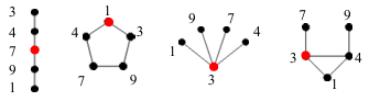
Similar to 3-node CISes, some 4-node CISes might be enumerated and counted more than once when we “pivoting" each node as above. To solve this problem, we propose the following methods for making sure each 4-node CIS is enumerated and gets counted once and only once: When and , we discard . Otherwise, denote by the associated undirected graph of by discarding edge labels. When includes one and only one node having at least 2 neighbors in , we let be the “responsible" of . For example, the node 4 is the “responsible" node of the first subgraph in Fig. 7. When includes more than one node having at least 2 neighbors in , we let the node with lowest order among the nodes having at least 2 neighbors in be the “responsible" node of . For example, the nodes 6 and 3 are the “responsible" nodes of the second and third subgraphs in Fig. 7.
4.3 5-node CIS Enumeration
Algorithm 4 describes our 5-node CISes enumeration method. For a 5-node CIS , we classify it into two types according to its associated undirected graph :
- •
5-node CIS with type 1: has at least one node having more than two neighbors in ;
- •
5-node CIS with type 2: has no node having more than two neighbors in , i.e., is isomorphic to a 5-node line or a circle, i.e., the first or sixth motifs in Fig. 4 (c).
We propose two different methods to enumerate these two types of 5-node CISes respectively.
To enumerate 5-node CISes with type 1, we “pivoting" each node as follows: When has at least three neighbors, we enumerate each combination of three nodes where , and then compute the neighborhood of , , , and , defined as . For any node , we observe that the induced graph consisting of nodes , , , , and is a 5-node CIS. Thus, we enumerate each node in , and update the associated 5-node CIS consisting of , , , , and . We repeat this process until all combinations of three nodes are enumerated and processed. Similar to 4-node CISes, we propose the following method to make sure each 5-node is enumerated and gets counted once and only once: When and , we discard . Otherwise, let be the associated undirected graph of , and we then pick the node with lowest order among the nodes having more than two neighbors in be the “responsible" node. The third and fourth subgraphs in Fig. 8 are two corresponding examples.
To enumerate 5-node CISes with type 2, we “pivoting" each node as follows: When has at least two neighbors, we first enumerate each pair of ’s neighbors and where . Then, we compute defined as the set of ’s neighbors not including and and not connecting to and , that is, . Similarly, we compute defined as the set of ’s neighbors not including and and not connecting to and , i.e., . Clearly, . For any and , we observe that the induced graph consisting of nodes , , , , and is a 5-node CIS with type 2. Thus, we enumerate each pair of and , and update the 5-node CIS consisting of , , , , and . We repeat this process until all pairs of ’s neighbors and are enumerated and processed. To make sure each CIS is enumerated and gets counted once and only once, we let the node with lowest order be the “responsible" node when the associated undirected graph of isomorphic to a 5-node circle. When is isomorphic to a 5-node line, we let the node in the middle of the line be the “responsible" node. The first and second subgraphs in Fig. 8 are two examples respectively.
| Graph | nodes | edges | max-degree |
|---|---|---|---|
| Flickr [21] | 1,715,255 | 15,555,041 | 27,236 |
| Pokec [30] | 1,632,803 | 22,301,964 | 14,854 |
| LiveJournal [21] | 5,189,809 | 48,688,097 | 15,017 |
| YouTube [21] | 1,138,499 | 2,990,443 | 28,754 |
| Wiki-Talk [15] | 2,394,385 | 4,659,565 | 100,029 |
| Web-Google [1] | 875,713 | 4,322,051 | 6,332 |
| soc-Epinions1 [25] | 75,897 | 405,740 | 3,044 |
| soc-Slashdot08 [18] | 77,360 | 469,180 | 2,539 |
| soc-Slashdot09 [18] | 82,168 | 504,230 | 2,552 |
| sign-Epinions [16] | 119,130 | 704,267 | 3,558 |
| sign-Slashdot08 [16] | 77,350 | 416,695 | 2,537 |
| sign-Slashdot09 [16] | 82,144 | 504,230 | 2,552 |
| com-DBLP [38] | 317,080 | 1,049,866 | 343 |
| com-Amazon [38] | 334,863 | 925,872 | 549 |
| p2p-Gnutella08 [26] | 6,301 | 20,777 | 97 |
| ca-GrQc [17] | 5,241 | 14,484 | 81 |
| ca-CondMat [17] | 23,133 | 93,439 | 279 |
| ca-HepTh [17] | 9,875 | 25,937 | 65 |
| Flickr | Pokec | LiveLive- | Wiki- | Web- | |
| Journal | Talk | ||||
| undirected 3-node motifs | |||||
| 1 | 9.60e-01 | 9.84e-01 | 9.55e-01 | 9.99e-01 | 9.81e-01 |
| 2 | 4.04e-02 | 1.60e-02 | 4.50e-02 | 7.18e-04 | 1.91e-02 |
| directed 3-node motifs | |||||
| 1 | 2.17e-01 | 1.77e-01 | 7.62e-02 | 8.91e-01 | 1.27e-02 |
| 2 | 6.04e-02 | 1.11e-01 | 4.83e-02 | 4.04e-02 | 1.60e-02 |
| 3 | 1.28e-01 | 1.60e-01 | 3.28e-01 | 3.91e-03 | 9.28e-01 |
| 4 | 2.44e-01 | 1.74e-01 | 1.14e-01 | 5.43e-02 | 3.09e-03 |
| 5 | 1.31e-01 | 1.91e-01 | 1.73e-01 | 5.48e-03 | 1.92e-02 |
| 6 | 1.80e-01 | 1.71e-01 | 2.15e-01 | 3.88e-03 | 1.92e-03 |
| 7 | 5.69e-05 | 7.06e-05 | 2.74e-05 | 1.37e-05 | 4.91e-05 |
| 8 | 6.52e-03 | 2.49e-03 | 8.66e-03 | 1.81e-04 | 6.82e-03 |
| 9 | 1.58e-03 | 1.03e-03 | 1.06e-03 | 8.42e-05 | 2.84e-04 |
| 10 | 5.19e-03 | 1.91e-03 | 6.63e-03 | 1.28e-04 | 2.77e-03 |
| 11 | 6.46e-03 | 2.03e-03 | 6.27e-03 | 8.03e-05 | 5.98e-03 |
| 12 | 1.07e-02 | 5.13e-03 | 9.82e-03 | 1.78e-04 | 1.21e-03 |
| 13 | 9.86e-03 | 3.45e-03 | 1.26e-02 | 6.65e-05 | 2.00e-03 |
| Flickr | Pokec | LiveLive- | Wiki- | Web- | |
| Journal | Talk | ||||
| 1 | 1.92e-03 | 3.26e-03 | 2.69e-03 | 5.21e-03 | 2.93e-04 |
| 2 | 4.56e-02 | 6.92e-02 | 1.64e-01 | 2.67e-01 | 4.00e-01 |
| 1 | 2.90e-04 | 4.10e-04 | 2.64e-04 | 6.06e-04 | 2.92e-05 |
| 2 | 6.90e-03 | 8.68e-03 | 1.61e-02 | 3.11e-02 | 3.99e-02 |
| sign-Epinions | sign-Slashdot08 | sign-Slashdot09 | |
|---|---|---|---|
| 1 | 6.69e-01 | 6.58e-01 | 6.68e-01 |
| 2 | 2.12e-01 | 2.32e-01 | 2.25e-01 |
| 3 | 9.09e-02 | 1.02e-01 | 9.96e-02 |
| 4 | 2.29e-02 | 5.86e-03 | 5.75e-03 |
| 5 | 2.76e-03 | 9.74e-04 | 9.34e-04 |
| 6 | 2.49e-03 | 1.14e-03 | 1.13e-03 |
| 7 | 3.81e-04 | 1.80e-04 | 1.76e-04 |
| soc- | soc- | soc- | com- | |
|---|---|---|---|---|
| Epinions1 | Slashdot08 | Slashdot09 | Amazon | |
| 1 | 3.24e-01 | 2.93e-01 | 2.90e-01 | 2.10e-01 |
| 2 | 6.15e-01 | 6.86e-01 | 6.89e-01 | 6.99e-01 |
| 3 | 2.78e-03 | 1.25e-03 | 1.30e-03 | 2.37e-03 |
| 4 | 5.45e-02 | 1.86e-02 | 1.84e-02 | 7.69e-02 |
| 5 | 3.01e-03 | 7.77e-04 | 8.48e-04 | 1.05e-02 |
| 6 | 2.25e-04 | 9.19e-05 | 9.36e-05 | 1.55e-03 |
| com-A | com- | p2p-Gn | ca- | ca-Con | ca- | |
|---|---|---|---|---|---|---|
| mazon | DBLP | utella08 | GrQc | dMat | HepTh | |
| 1 | 2.9e-2 | 1.4e-1 | 2.6e-1 | 9.8e-2 | 1.4e-1 | 2.6e-1 |
| 2 | 7.5e-1 | 1.8e-1 | 1.8e-1 | 5.2e-2 | 2.2e-1 | 8.2e-2 |
| 3 | 1.6e-1 | 4.4e-1 | 4.6e-1 | 2.1e-1 | 4.3e-1 | 4.4e-1 |
| 4 | 6.0e-3 | 4.8e-2 | 1.1e-2 | 1.0e-1 | 4.9e-2 | 6.0e-2 |
| 5 | 2.3e-3 | 1.1e-3 | 2.7e-2 | 1.4e-3 | 2.1e-3 | 5.4e-3 |
| 6 | 3.6e-5 | 5.0e-5 | 1.4e-3 | 9.2e-5 | 1.1e-4 | 4.1e-4 |
| 7 | 1.5e-2 | 5.6e-2 | 2.7e-2 | 1.1e-1 | 5.5e-2 | 6.4e-2 |
| 8 | 3.5e-2 | 7.9e-2 | 2.2e-2 | 1.2e-1 | 8.0e-2 | 5.2e-2 |
| 9 | 1.4e-3 | 4.2e-3 | 1.4e-3 | 1.5e-2 | 7.0e-3 | 8.4e-3 |
| 10 | 1.7e-4 | 1.4e-4 | 1.0e-3 | 6.5e-4 | 3.0e-4 | 8.0e-4 |
| 11 | 7.3e-3 | 8.1e-3 | 4.3e-3 | 2.3e-2 | 9.9e-3 | 1.0e-2 |
| 12 | 5.3e-4 | 6.4e-3 | 2.8e-4 | 2.3e-2 | 4.5e-3 | 3.6e-3 |
| 13 | 8.2e-5 | 3.5e-6 | 7.4e-4 | 4.5e-6 | 6.4e-6 | 3.5e-5 |
| 14 | 3.9e-4 | 5.2e-4 | 1.7e-4 | 2.8e-3 | 6.6e-4 | 1.0e-3 |
| 15 | 6.7e-4 | 2.6e-2 | 7.6e-5 | 1.5e-1 | 5.9e-3 | 5.3e-3 |
| 16 | 7.1e-4 | 3.4e-4 | 1.4e-4 | 1.4e-3 | 9.2e-4 | 4.4e-4 |
| 17 | 3.9e-5 | 1.1e-5 | 8.0e-5 | 4.3e-5 | 2.9e-5 | 8.4e-5 |
| 18 | 2.3e-5 | 4.9e-6 | 6.0e-6 | 2.3e-5 | 8.5e-6 | 3.0e-5 |
| 19 | 2.4e-4 | 2.8e-3 | 1.5e-5 | 1.9e-2 | 9.8e-4 | 5.8e-4 |
| 20 | 5.8e-5 | 4.2e-4 | 7.0e-7 | 8.0e-3 | 1.4e-4 | 8.2e-5 |
| 21 | 7.2e-6 | 7.9e-3 | 1.5e-8 | 6.1e-2 | 1.5e-4 | 3.2e-3 |
5 Evaluation
In this section, we first introduce our experimental datasets. Then we present results of experiments used to evaluate the performance of our method, Minfer, for characterizing CIS classes of size .
5.1 Datasets
We evaluate the performance of our methods on publicly available datasets taken from the Stanford Network Analysis Platform (SNAP)22 2 www.snap.stanford.edu, which are summarized in Table 2. We start by evaluating the performance of our methods in characterizing -node CISes over million-node graphs: Flickr, Pokec, LiveJournal, YouTube, Web-Google, and Wiki-talk, contrasting our results with the ground truth computed through an exhaustive method. It is computationally intensive to calculate the ground-truth of -node and -nodes CIS classes in large graphs. For example, we can easily observe that a node with degree is included in at least 4-node CISes and 5-node CISes, therefore it requires more than and operations to enumerate the 4-node and 5-node CISes of the Wiki-talk graph, which has a node with 100,029 neighbors. Even for a relatively small graph such as soc-Slashdot08, it takes almost 20 hours to compute all of its 4-node CISes. To solve this problem, the experiments for 4-node CISes are performed on four medium-sized graphs soc-Epinions1, soc-Slashdot08, soc-Slashdot09, com-DBLP, and com-Amazon, and the experiments for 5-node CISes are performed on four relatively small graphs ca-GR-QC, ca-HEP-TH, ca-CondMat, and p2p-Gnutella08, where computing the ground-truth is feasible. We also evaluate the performance of our methods for characterizing signed CIS classes in graphs sign-Epinions, sign-Slashdot08, and sign-Slashdot09.
5.2 Error Metric
In our experiments, we focus on the normalized root mean square error (NRMSE) to measure the relative error of the estimator of the subgraph class concentration , . is defined as:
where is defined as the mean square error (MSE) of an estimate with respect to its true value , that is
We note that decomposes into a sum of the variance and bias of the estimator . Both quantities are important and need to be as small as possible to achieve good estimation performance. When is an unbiased estimator of , then we have and thus is equivalent to the normalized standard error of , i.e., . Note that our metric uses the relative error. Thus, when is small, we consider values as large as to be acceptable. In all our experiments, we average the estimates and calculate their NRMSEs over 1,000 runs.
5.3 Accuracy Results
5.3.1 Accuracy of inferring 3-node motifs’ concentrations
Table 3 shows the real values of the 3-node undirected and directed motifs’ concentrations for the undirected graphs and directed graphs of Flickr, Pokec, LiveJournal,Wiki-Talk, and Web-Google. Among all 3-node directed motifs, the 7-th motif exhibits the smallest concentration for all these five directed graphs. Here the undirected graphs are obtained by discarding the edge directions of directed graphs. Flickr, Pokec, LiveJournal,Wiki-Talk, and Web-Google have , , , , and 3-node CISes respectively. Table 4 shows the NRMSEs of our estimates of 3-node undirected motifs’ concentrations for and respectively. We observe that the NRMSEs associated with the sampling probability is about ten times smaller than the NRMSEs when . The NRMSEs are smaller than 0.04 when for all five graphs. Fig. 9 shows the NRMSEs of our estimates of 3-node directed motifs’ concentrations for and respectively. Similarly, we observe the NRMSEs when are nearly ten times smaller than the NRMSEs when . The NRMSE of our estimates of (i.e., the 7-th 3-node directed motif concentration) exhibits the largest error. Except for , the NRMSEs of the other motif concentrations’ estimates are smaller than 0.2 when .
Table 5 shows the real values of 3-node signed motifs’ concentrations for Sign-Epinions, sign-Slashdot08, and sign-Slashdot09. Sign-Epinions, sign-Slashdot08, and sign-Slashdot09 have , , and 3-node CISes respectively. Fig. 10 shows the NRMSEs of our estimates of 3-node signed and undirected motifs’ concentrations for and respectively. For all these three signed graphs, the NRMSEs are smaller than 0.9 and 0.2 when and respectively.
5.3.2 Accuracy of inferring 4-node motifs’ concentrations
Table 6 shows the real values of , i.e., the concentrations of 4-node undirected motifs for Soc-Epinions1, soc-Slashdot08, soc-Slashdot09, and com-Amazon. Soc-Epinions1, soc-Slashdot08, soc-Slashdot09, and com-Amazon have , , , and 4-node CISes respectively. Fig. 11 shows the NRMSEs of , the concentration estimates of 4-node undirected motifs for , , and respectively. We observe that motifs with smaller exhibit larger NRMSEs. Except , the NRMSEs of the other motif concentrations’ estimates are smaller than 0.2 for .
5.3.3 Accuracy of inferring 5-node motifs’ concentrations
Table 7 shows the real values of , i.e., the concentrations of 5-node undirected motifs for com-Amazon, com-DBLP, p2p-Gnutella08, ca-GrQc, ca-CondMat, and ca-HepTh. Com-Amazon, com-DBLP, p2p-Gnutella08, ca-GrQc, ca-CondMat, and ca-HepTh contains , , , , , and 5-node CISes respectively. Fig. 12 shows the NRMSEs of , the concentration estimates of 5-node undirected motifs for , , and respectively. We observe that NRMSE decreases as increases, and the 6-th, 10-th, 13-th, 17-th, 18-th 5-node motifs with small exhibit large NRMSEs.
5.4 Error Bounds
Figure 13 shows the root CRLBs (RCRLBs) and the root MSEs (RMSEs) of our estimates of 3-node directed motifs’ concentrations, 4-, and 5-node undirected motifs’ concentrations, where graphs LiveJournal, soc-Epinions, and com-DBLP are used for studying 3-node directed motifs, 4-, and 5-node undirected motifs respectively. We observe that the RCRLBs are smaller than the RMSEs, and fairly close to the RMSEs. The and RCRLBs are almost indistinguishable for 3-node directed motifs, where and LiveJournal is used. It indicates that the RCRLBs can efficiently bound the errors of our motif concentration estimations.
6 Related Work
There has been considerable interest to design efficient sampling methods for counting specific subgraph patterns such as triangles [31, 23, 12, 2], cliques [6, 9], and cycles [19], because it is computationally intensive to compute the number of the subgraph pattern’s appearances in a large graph. Similar to the problem studied in [13, 37, 22, 4, 36], in this work we focus on characterizing 3-, 4-, and 5-nodes CISes in a single large graph, which differs from the problem of estimating the number of subgraph patterns appearing in a large set of graphs studied in [10]. OmidiGenes et al. [22] proposed a subgraph enumeration and counting method using sampling. However this method suffers from unknown sampling bias. To estimate subgraph class concentrations, Kashtan et al. [13] proposed a subgraph sampling method, but their method is computationally expensive when calculating the weight of each sampled subgraph, which is needed to correct for the bias introduced by sampling. To address this drawback, Wernicke [37] proposed an algorithm, FANMOD, based on enumerating subgraph trees to detect network motifs. Bhuiyan et al. [4] proposed a Metropolis-Hastings based sampling method GUISE to estimate 3-node, 4-node, and 5-node subgraph frequency distribution. Wang et al. [36] proposed an efficient crawling method to estimate online social networks’ motif concentrations, when the graph’s topology is not available in advance and it is costly to crawl the entire topology. In summary, previous methods focus on designing efficient sampling methods and crawling methods for estimating motif statistics when the graph is directly available or indirectly available (i.e., it is not expensive to query a node’s neighbors [36]). They cannot be applied to solve the problem studied in this paper, i.e., we assume the graph is not available but a RESampled graph is given and we aim to infer the underlying graph’s motif statistics from the RESampled graph. At last, we would like to point out our method of estimating motif statistics and its error bound computation method are inspired by methods of estimating flow size distribution for network traffic measurement and monitoring [8, 24, 32, 35].
7 Conclusions
To the best of our knowledge, we are the first to study the problem of inferring the underlying graph’s motif statistics when the entire graph topology is not available, and only a RESampled graph is given. We propose a model to bridge the gap between the underlying graph’s and its RESampled graph’s motif statistics. Based on this probabilistic model, we develop a method Minfer to infer the underlying graph’s motif statistics, and give a Fisher information based method to bound the error of our estimates. and experimental results on a variety of known data sets validate the accuracy of our method.
Appendix
The matrixes and is shown in Fig. 14.
Acknowledgment
We thank the anonymous reviewers as well as Dr. Wei Fan for helpful suggestions.
References
- [1] Google programming contest. http://www.google.com/programming-contest/, 2002.
- [2] N. Ahmed, N. Duffield, J. Neville, and R. Kompella. Graph sample and hold: A framework for big-graph analytics. In Proceedings of the 20th ACM SIGKDD International Conference on Knowledge Discovery and Data Mining, pages 589–597, 2014.
- [3] I. Albert and R. Albert. Conserved network motifs allow protein–protein interaction prediction. Bioinformatics, 4863(13):3346–3352, 2004.
- [4] M. A. Bhuiyan, M. Rahman, M. Rahman, and M. A. Hasan. Guise: Uniform sampling of graphlets for large graph analysis. In Proceedings of IEEE ICDM 2012, pages 91–100, December 2012.
- [5] J. Chen, W. Hsu, M.-L. Lee, and S.-K. Ng. Nemofinder: dissecting genome-wide protein-protein interactions with meso-scale network motifs. In Proceedings of ACM SIGKDD 2006, pages 106–115, August 2006.
- [6] J. Cheng, Y. Ke, A. W.-C. Fu, J. X. Yu, and L. Zhu. Finding maximal cliques in massive networks. ACM Transactions on Database Systems, 36(4):21:1–21:34, dec 2011.
- [7] H. Chun, Y. yeol Ahn, H. Kwak, S. Moon, Y. ho Eom, and H. Jeong. Comparison of online social relations in terms of volume vs. interaction: A case study of cyworld. In Proceedings of ACM SIGCOMM Internet Measurement Conference 2008, pages 57–59, November 2008.
- [8] N. Duffield, C. Lund, and M. Thorup. Estimating flow distributions from sampled flow statistics. In Proceedings of ACM SIGCOMM 2003, pages 325–336, August 2003.
- [9] M. Gjoka, E. Smith, and C. T. Butts. Estimating Clique Composition and Size Distributions from Sampled Network Data. ArXiv e-prints, Aug. 2013.
- [10] M. A. Hasan and M. J. Zaki. Output space sampling for graph patterns. In Proceedings of the VLDB Endowment 2009, pages 730–741, August 2009.
- [11] S. Itzkovitz, R. Levitt, N. Kashtan, R. Milo, M. Itzkovitz, and U. Alon. Coarse-graining and self-dissimilarity of complex networks. Physica Rev.E, 71:016127, 2005.
- [12] M. Jha, C. Seshadhri, and A. Pinar. A space efficient streaming algorithm for triangle counting using the birthday paradox. In Proceedings of the 19th ACM SIGKDD International Conference on Knowledge Discovery and Data Mining, pages 589–597, 2013.
- [13] N. Kashtan, S. Itzkovitz, R. Milo, and U. Alon. Efficient sampling algorithm for estimating subgraph concentrations and detecting network motifs. Bioinformatics, 20(11):1746–1758, 2004.
- [14] J. Kunegis, A. Lommatzsch, and C. Bauckhage. The slashdot zoo: mining a social network with negative edges. In Proceedings of WWW 2009, pages 741–750, April 2009.
- [15] J. Leskovec, D. Huttenlocher, and J. Kleinberg. Predicting positive and negative links in online social networks. In Proceedings of WWW 2010, pages 641–650, April 2010.
- [16] J. Leskovec, D. Huttenlocher, and J. Kleinberg. Signed networks in social media. In Proceedings of the 28th ACM Conference on Human Factors in Computing Systems (CHI), pages 1361–1370, April 2010.
- [17] J. Leskovec, J. Kleinberg, and C. Faloutsos. Graph evolution: Densification and shrinking diameters. Transactions on Knowledge Discovery from Data (TKDD), 1(1), Mar. 2007.
- [18] J. Leskovec, K. J. Lang, A. Dasgupta, and M. W. Mahoney. Community structure in large networks: Natural cluster sizes and the absence of large well-defined clusters. Internet Mathematics, 6(1):29–123, 2009.
- [19] M. Manjunath, K. Mehlhorn, K. Panagiotou, and H. Sun. Approximate counting of cycles in streams. In Proceedings of the 19th European Conference on Algorithms, ESA’11, pages 677–688, Berlin, Heidelberg, 2011. Springer-Verlag.
- [20] R. Milo, E. Al, and C. Biology. Network motifs: Simple building blocks of complex networks. Science, 298(5549):824–827, October 2002.
- [21] A. Mislove, M. Marcon, K. P. Gummadi, P. Druschel, and B. Bhattacharjee. Measurement and analysis of online social networks. In Proceedings of ACM SIGCOMM Internet Measurement Conference 2007, pages 29–42, October 2007.
- [22] S. Omidi, F. Schreiber, and A. Masoudi-nejad. Moda: An efficient algorithm for network motif discovery in biological networks. Genes and Genet systems, 84(5):385–395, 2009.
- [23] A. Pavany, K. T. S. Tirthapuraz, and K.-L. Wu. Counting and sampling triangles from a graph stream. In Proceedings of VLDB, pages 1870–1881, 2013.
- [24] B. Ribeiro, D. Towsley, T. Ye, and J. Bolot. Fisher information of sampled packets: an application to flow size estimation. In Proceedings of ACM SIGCOMM IMC 2006, pages 15–26, October 2006.
- [25] M. Richardson, R. Agrawal, and P. Domingos. Trust management for the semantic web. In Proceedings of the 2nd International Semantic Web Conference, pages 351–368, October 2003.
- [26] M. Ripeanu, I. T. Foster, and A. Iamnitchi. Mapping the gnutella network: Properties of large-scale peer-to-peer systems and implications for system design. IEEE Internet Computing Journal, 6(1):50–57, 2002.
- [27] T. Schank. Algorithmic Aspects of Triangle-Based Network Analysis. PhD thesis, 2007.
- [28] S. S. Shen-Orr, R. Milo, S. Mangan, and U. Alon. Network motifs in the transcriptional regulation network of escherichia coli. Nature Genetics, 31(1):64–68, May 2002.
- [29] S. Suri and S. Vassilvitskii. Counting triangles and the curse of the last reducer. WWW 2011, pages 607–614, 2011.
- [30] L. Takac and M. Zabovsky. Data analysis in public social networks. In International Scientific Conference and International Workshop Present Day Trends of Innovations, pages 1–6, May 2012.
- [31] C. E. Tsourakakis, U. Kang, G. L. Miller, and C. Faloutsos. Doulion: Counting triangles in massive graphs with a coin. In PROCEEDINGS OF ACM KDD 2009, 2009.
- [32] P. Tune and D. Veitch. Towards optimal sampling for flow size estimation. In Proc. of the IMC, pages 243–256, 2008.
- [33] J. Ugander, L. Backstrom, and J. Kleinberg. Subgraph frequencies: mapping the empirical and extremal geography of large graph collections. In Proceedings of the 22nd international conference on World Wide Web, WWW 2013, pages 1307–1318, 2013.
- [34] H. L. van Trees. Estimation and Modulation Theory, Part 1. Wiley, New York, 2001.
- [35] P. Wang, X. Guan, J. Zhao, J. Tao, and T. Qin. A new sketch method for measuring host connection degree distribution. IEEE Transactions on Information Forensics and Security, 9(6):948–960, 2014.
- [36] P. Wang, J. C. Lui, J. Zhao, B. Ribeiro, D. Towsley, and X. Guan. Efficiently estimating motif statistics of large networks. ACM Transactions on Knowledge Discovery from Data, 2014.
- [37] S. Wernicke. Efficient detection of network motifs. IEEE/ACM Transactions on Computational Biology and Bioinformatics, 3(4):347–359, 2006.
- [38] J. Yang and J. Leskovec. Defining and evaluating network communities based on ground-truth. In 12th IEEE International Conference on Data Mining (ICDM), pages 745–754, 2012.
- [39] J. Zhao, J. C. S. Lui, D. Towsley, X. Guan, and Y. Zhou. Empirical analysis of the evolution of follower network: A case study on douban. In Proceedings of IEEE INFOCOM NetSciCom 2011, pages 941–946, April 2011.