Holographic codes
Abstract
There exists a remarkable four-qutrit state that carries absolute maximal entanglement in all its partitions. Employing this state, we construct a tensor network that delivers a holographic many body state, the H-code, where the physical properties of the boundary determine those of the bulk. This H-code is made of an even superposition of states whose relative Hamming distances are exponentially large with the size of the boundary. This property makes H-codes natural states for a quantum memory. H-codes exist on tori of definite sizes and get classified in three different sectors characterized by the sum of their qutrits on cycles wrapped through the boundaries of the system. We construct a parent Hamiltonian for the H-code which is highly non local and finally we compute the topological entanglement entropy of the H-code.
We introduce the concept of a holographic code as a balanced superposition of quantum states for which boundary and bulk degrees of freedom are strictly related
| (1) |
where the states form a product basis of the Hilbert space of the boundary made of degrees of freedom of dimension , and are orthogonal product states in the bulk, . Let us emphasize that all and are product states, at variance with the structure of the standard Schmidt decomposition where such states are not necessarily product states. We shall also construct substates of a holographic code, that will be characterized by observables that test the topology of the state. A good property for a holographic code will later be characterized by large Hamming distances among all elements , so that distinguishability of each individual element is maximized.
It follows from the basic definition in Eq.(1) that the scaling of entanglement entropy in orthogonal holographic codes is bounded by an area law. This upper bound emerges trivially from the fact that the total amount of superpositions for any partition of the system is bounded by . This key feature is guarantee by the balanced superposition of states and the fact that the bulk states are all product states.
Tensor network construction of an orthogonal holographic code.– Let us consider a quantum system made of qutrits on an infinite triangular lattice in 2D. We shall now define a tensor network that gives rise to a class of orthogonal holographic states.
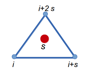
The basic idea is to construct a network of triangular simplices on triangles pointing up, where ancillary qutrits live. Then a physical qutrit index is dictated by the values of the underlying ancillary indices. The construction is illustrated in Fig. 1. The specific assignment for each physical qutrit is made as follows
| (2) |
where the index corresponds to the physical index, and all qutrit indices live in and are to be considered mod(3). This construction is tantamount to set up a PEPS-like tensor network based on the translational invariant tensor which is 1 if and and 0 otherwise. The rational for this construction is that such a state is an example of absolute maximal entanglement [1].
Let us note that the existence of absolute maximally entangled states is non-trivial [2]. For instance, there are no four-qubit states that have such a property. It is possible to construct absolute maximally entangled states related to Reed-Solomon codes, which only appear for certain local dimensions and number of local Hilbert spaces [1]. The four-qutrit state Eq.(2) we use in our construction is the first non-trivial maximally entangled state for four local degrees of freedom, that is, the first fully entangled generalization of EPR states to the four-body case.
The first relevant property of the state Eq.(2) we have taken as the underlying structure of the tensor network is that it provides a mapping of a 2-qutrit basis onto a related but different 2-qutrit basis. Indeed, the indices and span the natural basis for two qutrits and and produce a second basis. Therefore, given the value of two qutrits, the other two are fixed, at variance with traditional Projected Entangled Pairs States (PEPS) where two indices do not fully determine the other two [3, 5]. Therefore, in our construction, fixing a first raw of physical indices and a unique ancilla, the rest of the network, including all physical indices, is fixed. Furthermore, this construction is also valid as seen from the diagonal directions, since the property of absolute maximal entanglement guarantees that it is always possible to view the network assignment as a mapping between basis, no matter which partition of the four indices is made.
The second relevant property emerging from the absolute maximally entangled state of Eq.(2) is that the second row in the network of physical indices is completely determined in a simple way. It is easy to check that if two physical indices on a first raw are taken to be and , then they force the physical index in the second raw to be (see Eq.(3)). This is tantamount to define the upper physical index by imposing that the total sum of indices is zero, where we always work mod 3 because of the qutrit nature of the local Hilbert spaces. This systematic enforcement of the values of all physical indices proceeds as more rows are added to the network as shown in Fig. 2, so that a perfect holographic state emerges. All the elements in the bulk are determined from the qutrits in the boundary.

At this point of the construction of the holographic state it is possible to dispose of the underlying ancillary structure. The net effect of the ancillary states was to obtain a state based on the simple rule that every triangle of physical indices must add up to zero mod 3, namely
| (3) |
We shall call this property the neutralization rule. Once this neutralization rule is deduced, it suffices to produce all the state as if we were dealing with a cellular automaton operation. Given the first row of qutrits , the complete state is represented by
| (4) |
where delivers the values of each qutrit in the bulk using repeatedly the neutralization rule. It is clear that this neutralization rule acts as a cellular automata defining a row at a time. Every physical qutrit is defined by its predecessors that form a sort of backwards light-cone.
Let us note that all states based on homogeneous tensor networks, such as translational invariant PEPS [3]-[7], are holographic, in the sense that the value of the boundary ancillae determine a superposition state in the bulk. This also applies to the H-state since it is also determined by the simplex structure of the ancillae. However, the difference is that standard tensor networks are such that orthogonal states on the boundary produce non-orthogonal states in the bulk, while in our case orthogonality in the bulk is preserved. Moreover, we shortly prove that the neutralization rule enforces a topological structure absent in usual PEPS.
From now on we shall refer to the superposition state
| (5) |
as a H-code, standing for our orthogonal holographic code. Note that is the length of the boundary and the bulk can extend to a number of rows that depends on the topology of the system.
H-code on a torus.– It is not obvious that the H-code can be defined on lattices with non trivial topologies such as the torus. The reason is that the neutralization rule defines every layer of the state and may be not allow for periodic boundary conditions.
The solution to this riddle is somewhat surprising. We shall now see that H-codes can be defined on a torus of size only for certain values of and . In particular, there is a H-code for every torus . To obtain this result, let us consider Fig. 2. Periodicity will be allowed if a consistent identification of spins along the rows and columns is possible. Let us focus on the first qutrit of each row and notice that in the fourth row we find it to be . This allows for the assignment that brings , thus providing exact periodicity both in the diagonal and the row for the case .
For larger tori, a scale symmetry emerges. It is easy to see that the tenth row first qutrit reads . Then, the identification yields again perfect periodicity for since . This pattern linking the horizontal period with the diagonal one is repeated for every with (see Supplementary material). It is possible to find other periodic H-codes in the holographic dimension depending on the values of . For instance, we have found valid H-codes on tori . For other cases, only a subsector of the boundary Hilbert space can yield periodic sates. In the following, we shall stick to the squared tori with size with perfect periodicity.
There is a further relevant property found on H-codes on a torus. It is easy to verify that for sizes , the product of the qutrit values on every horizontal line as well as every diagonal line is equal to
| (6) |
where each can take values 1, or , corresponding to the spins , with . As a consequence, a sub-structure of states within the H-code into three categories emerges, each one labelled by a different value of . Such a property hints at the possibility of using topological H-code as a quantum memory.
Hamming distance for the H-code.– It is interesting to see how a H-code state can store information. Given the cellular automata character of the neutralization rule, any change of a given qutrit propagates a modification of the state on a sort of light-cone which is contained within the diagonals emerging from that point upwards. This propagation of changes is necessary to preserve the neutralization rule Eq.(3). If a single qutrit is changed in the boundary, then every row in the bulk needs to be changed.
It is possible to verify that any two states in the H-code on a torus of size , differ at least by elements. That is, the minimum Hamming distance between any pair of elements in the code is . This property makes the elements of the code easily distinguishable, which provides a way to code information in a very redundant manner. As an example, for a code, there are a total of states, as defined in the 9 qutrit boundary. Then, in the large Hilbert space made of 81 qutrits, all the elements in the superposition differ at least by a Hamming distance of .
The relevant point is that H-codes provides exponential distinguishability as the size of the torus increases. Furthermore, non-orthogonal holographic codes such as PEPS do not allow for easy distinguishability, since bulk configurations are not orthogonal.
Construction of a H-code.– The simplest way to generate a H-code is to guarantee a superposition of elements in the boundary and then set the rest of elements using a cellular automata strategy. We first encode the previous index as an exponent, so as to implement the qutrit nature of the local physical system. That is gives rise to for , for and for .
We choose as boundary Hamiltonian
| (7) |
where the sum over runs through the qutrits in the boundary and
| (8) |
acts as a raising operator (note that . The idea behind this choice of boundary Hamiltonian is that it performs a generalized symmetrization of every pair of qutrits while preserving their sum, that is, it maps (00,12,21) onto (00+12+21), (01,22,10) onto (01+22+10) and (02,11,20) onto (02+11+20). Note that the symmetrization implied by makes it relevant to take open or periodic boundary conditions.
We can now propagate this superposition into a bulk using the following cellular automata strategy. For each layer we act on contiguous qutrits using the unitary operator
| (9) |
which can be created using the circuit in Fig. 3.

The construction we have provided, based on a boundary Hamiltonian and a cellular automata, has three distinct ground states
| (10) |
labeled by the sum of the qutrits on any row or diagonal , which corresponds to . This shows that the H-code is able to codify one qutrit state through properties related to observables spanning through boundaries of the system. The fact that takes the same value on every row and every diagonal and the large Hamming distance among all superpositions in the H-code suggests that the coding of states is robust against some local fluctuations.
Parent Hamiltonian.– Tensor network states have the property of being the ground states of the so called parent Hamiltonians. They do not have to be unique. For the H-code there is a huge freedom (see Suplementary material). The simplest case is made of two terms
| (11) |
The first term reads
| (12) |
where
| (13) |
The sum runs over all the spins located at the corners of the up triangles of the lattice. One can easily verify that vanishes if and only if . In the remaining cases for each violation of the neutrality rule Eq.(3). The Hamiltonian (12) is highly degenerate since any configuration satisfying Eq.(3) will be a ground state. To break this degeneracy we consider the operator (see Suplementary material)
| (14) |
where denotes the operator (8) acting on the site of the torus. contains a pair of operators and per each up triangle, and an equal number of and per row or column. These properties imply that commutes with and , hence the ground states of satisfy the neutrality rule, that minimizes , and have a definite value of . In these subspace of states, is a non positive matrix and then the Perron-Frobenius theorem yields that the ground state is the H-code Eq.(10) with . is a highly non local operator that contains products of matrices . This non locality is due to the exponential increase of the Hamming distance that grows as . One may speculate that non local Hamiltonians such as (14) may arise from integrating some gauge degree of freedom.
Entanglement entropy and topological entropy.– Entanglement entropy remains a natural way to quantify the amount of quantum correlations in a given state [8, 9]. It turns out that an exact computation of the entanglement entropy for the H-code is easily done. Let us first consider the simplest situation with three qutrits forming a triangle as in Fig. 1, and let us call them , and . Qutrits and are free to take any value, but qutrit is dictated by the neutralization rule, since and are its backward light-cone. Then
| (15) |
where we have decided to measure entropies using base 3, given the qutrit structure of the H-code. Similarly, for any close region made of qutrits, we must count how many of them are free vs. those who are dictated by the neutralization rule. So, if independent qutrits appear in the boundary, the entropy will be
| (16) |
This reasoning is now sufficient to compute the topological entropy as follows. Consider again the case of a triangle made with three qutrits , and , and let us call the rest of the system . Then the topological entropy will be given by [8, 9]
| (17) | |||||
This extends to any configuration of contiguous , and since it is easy to show that adding one qutrit at a time in any position around a given configuration preserves the value of .
The three possible states of the H-code on a torus, that is , cannot be distinguished using bulk observables. The reduced density matrix of any subset made out of bulk qutrits, with is simply , that is is fully disordered. In the case that the number of qutrits appearing in is larger than the size of the boundary of the torus, there are not sufficient degrees of freedom to achieved maximum entropy. Then, an area law appears for the entropy
Conclusions.– We have introduced the concept and explicit construction of a holographic code which is characterized by an exact mapping of boundary states onto bulk ones. This mapping is achieved by a neutralization rule which is related to the ground state of a two-body nearest neighbour Hamiltonian. The construction of a symmetric state on the boundary produces a H-code on the bulk of a torus which can encode a qutrit through its topological properties.
In general, an H-code can be viewed as a compressor of bulk states that uses a basis of elements whose Hamming distances are large. Alternatively, an H-code makes redundant the information of its boundary by disseminating it through the bulk of the system.
Acknowledgements.– We thank D. Cabra, J. I. Cirac, S. Iblisdir, J. Pachos, N. Schuch and F. Verstraete for their comments. We acknowledge financial support from FIS2013-41757-P, FIS-2012-33642, QUITEMAD, and the Severo Ochoa Programme under grant SEV-2012-0249.
References
- [1] W. Helwig, W. Cui, A. Riera, J. I. Latorre and H-K. Lo, Phys. Rev. A 86, 052335 (2012); arXiv:1204.2289. D. Goyeneche and K. ZyczkowskiarXiv, arXiv:1404.3586.
- [2] G. Gour and N. R. Wallach, Journal of Mathematical Physics 51:112201 (2011). arXiv:quant-ph/1006.0036.
- [3] F. Verstraete and J. I. Cirac, arXiv:cond-mat/0407066.
- [4] D. Pérez-García, F. Verstraete, J. I. Cirac, Michael M. Wolf, Quant. Inf. Comp. 8, 0650-0663 (2008); arXiv:0707.2260.
- [5] J. I. Cirac, F. Verstraete, J. Phys. A: Math. Theor. 42, 504004 (2009); arXiv:0910.1130.
- [6] J. I. Cirac, D. Poilblanc, N. Schuch, F. Verstraete, Phys. Rev. B 83, 245134 (2011); arXiv:1103.3427.
- [7] R. Orús, Annals of Physics 349,117 (2014); arXiv:1306.2164.
- [8] A. Kitaev and J. Preskill, Phys. Rev. Lett. 96, 110404 (2006); arXiv:hep-th/0510092.
- [9] M. Levin and X. G. Wen, Phys. Rev. Lett. 96, 110405 (2006); arXiv:cond-mat/0510613.
Suplementary Material
H-Codes on the torus–
Let us consider a torus of size . Using the neutralization rule Eq. (3), the map from row-to-row states can be represented as
| (18) |
where (mod 3). The transfer matrix defined in this way reads
| (19) |
where is the -dimensional identity matrix and
| (20) |
satisfies
| (21) |
A -code on the torus is possible if after iterations of any state on the first row returns to itself. This situation is guaranteed if and only if
| (22) |
Let us show that this condition holds for . Using Eq. (19)
where we have used Eq.(21) and the fact that is divisible by 3, for with . This example shows that finding consistent -codes is an interesting problem in modular arithmetic.
Injectivity and parent Hamiltonian–
Let us represent the PEPS-like tensor as
| (26) |
where indicates the ancilla indices and the triangle is associated to the spin . On the plane one can construct two generic types of networks labeled by an integer . The networks for are
| (27) |
and
| (28) |
and their type will be denoted and respectively. Both networks have triangles aligned on the edges, and a total of triangles, that is spins. In the networks of type all the internal ancillas are contracted in groups of three using the GHZ state, while in the networks the ancillas on the edges are contracted using a Bell state. These networks differ in the fact that for the -type the values of the spins on a single edge determine holographically the remaining spins, while for the -type one needs the values of the spins on two edges.
Let us study the injectivity properties of these tensor networks. PEPS is injective if the map constructed with a tensor network between the ancilla indices and the physical indices is injective [4]. Here the ancillas refer to the ones that are left uncontracted or open. Recall that a linear map is injective if the kernel of is empty.
To analyze this property we choose the networks whose internal ancillas are all contracted while the external ones are open. There is a total of outgoing ancillas, but they are not all independent: fixing ancillas on two boundaries determine the values of the remaing outer ancillas and all the spins. This implies that the map from the outgoing ancillas and the spins has a non trivial kernel, hence the map is not injective. The same happens for the networks of type . For MPS the injectivity property guarantees the uniqueness of the ground state of the parent Hamiltonian but not for PEPS [4]. Nevertheless we construct below a parent Hamiltonian whose ground state on the torus has only the degeneracy due to the charge of Eq.(6).
First notice that the neutralization rule Eq. (3) is satisfied by all the ground states of the Hamiltonian (recall Eq.(12) )
| (29) |
where is defined in Eq.(13). The proof is as follows. The solutions of Eq.(3) are: 1) that corresponds to equal to in which case and so ; and 2) (and permutations) that also leads to and . In the remaining cases where (3) is not satisfied one finds that for each frustrated triangle.
Let us construct an operator that mixes the states satisfying Eq.(3). First we consider the state on the torus with sites
| (30) |
labels the spins . Eq.(3) is satisfied on each triangle, e.g. . Let us now consider the operator
| (31) | |||
which satisfies
| (32) |
because the operators and appear in each triangle and therefore their product commutes with (notice that . also commutes with the charge ,
| (33) |
which implies that and can be diagonalized simultaneously. To find the ground state of we first minimize that yields the states satisfying the neutralization rule Eq.(3) (recall Eq.(4))
Now, we diagonalize in the subspace with ,
where it acts as
This is a matrix whose eigenvalues (degeneracies) are : . The ground state, i.e. , is given by
| (34) |
The uniqueness of this state and the fact that all its entries have the same sign follows from the Perron-Frobenius theorem applied to the non-positive matrix , in the subspace .
How unique is the operator (31)? To answer this question we shall consider the general expression
| (35) |
and impose the condition (32) that yields
| (36) |
which is solved by
| (37) |
This is a linear system of 9 equations for 9 unknowns. The rank of the corresponding matrix is 2. Choosing 0 in the RHS of Eq.(37) and imposing translation invariance leads to the ansatz (31). Finally, the sign of the constants guarantees that (34) are GS’s. Allowing the RHS of Eq.(37) to take the values 0 and yields another solutions as for example
| (38) | |||
However, this operator does not commute with the charge , so that the ground state of is unique and given by
| (39) |
A generalization of the Hamiltonian (31) to the torus , with is given in Eq.(14). One can easily verify that this Hamiltonian satisfies Eqs.(32) and (33), with given in Eq.(6). The Hamiltonian (14) contains local operators , which for amounts to 54. However it is possible to construct Hamiltonians with a small number of terms, say 36 for , which satisfy Eqs.(32) and (33). Notice that 36 coincides with the Hamming dimension for , hence we expect the existence of parent Hamiltonians containing exactly local terms .
Finally, we want to remark that the neutralization rule can be extended to operators. Indeed, let us consider the following operator defined on the boundary of the torus
| (40) |
which modifies the state on the boundary as
| (41) |
The state on the second row can be obtained applying the neutralization rule to the RHS of (41),
| (42) |
but this state can also be obtained acting on with the operator
Proceeding in this manner one can associate an operator in the bulk to any boundary operator (40) on the edge. In fact Eqs.(38) and (38) provide examples of this holographic extension of operators.