Phase diagram of the ST2 model of water

To evaluate the fluid free energy we perform thermodynamic integration along a path of constant reference density $\rho_{\mathrm{ref}}$ for a modified pair potential,

$$V=\min(V_{ST2},200\mathrm{\;kJ/mol}).$$

(1)

This potential coincides with the ST2 potential for all intermolecular distances and orientations where $V_{ST2}<200$ kJ/mol, and is constant and equal to 200 kJ/mol otherwise. Note that in the temperature range where we investigate the phase behavior, molecules never approach close enough to reach this limit. In this way, the divergence of the potential energy for configurations in which some intermolecular separations vanish (which would otherwise be probed at very high temperatures) is eliminated and the infinite temperature limit is properly approximated by an ideal gas of molecules at the same density.

The fluid free energy (per particle) is calculated as

$$\beta f_{ST2}^{\mathrm{fluid}}(\beta,\rho_{\mathrm{ref}})=\beta f_{\mathrm{ig}}(\beta,\rho_{\mathrm{ref}})+\int_{0}^{\beta}\left\langle V(\beta,\rho_{\mathrm{ref}})\right\rangle d\beta,$$

(2)

where $\beta=1/k_{B}T$ and $\beta f_{\mathrm{ig}}(\beta,\rho)=\log(\rho_{n}\sigma^{3})-1$ is the ideal gas free energy and $\rho_{n}$ is the number density. Fig. 1 shows the average modified pair potential energy $\left\langle V(\beta,\rho)\right\rangle$ and the interpolating (spline) continuous curve used to numerically evaluate the integral. The free energy at different densities along a constant-$T$ path is evaluated via thermodynamic integration of the equation of state

$$\beta f_{ST2}^{\mathrm{fluid}}(T,\rho_{n})=\beta f_{ST2}^{\mathrm{fluid}}(T,\rho_{n,\mathrm{ref}})+\int_{\rho_{n,\mathrm{ref}}}^{\rho_{n}}\frac{\beta P(\rho_{n}^{\prime})}{\rho_{n}^{\prime}}d\ln(\rho_{n}^{\prime}),$$

(3)

where $P(\rho_{n})$ is the equation of state for the pressure $P$ at fixed $T$.

To evaluate the free energy of a selected crystalline structure we follow the methodology reviewed in Ref. [31]. We define an Einstein crystal in which each molecule interacts, in addition to the ST2 potential, with a Hamiltonian, composed of a translational ($H_{\mathrm{trans}}$) and a rotational ($H_{\mathrm{rot}}$) part, that attaches each molecule to a reference position and orientation. For each particle we define two unit vectors: the (normalized) HH vector and dipole vector, named respectively $\vec{a}$ and $\vec{b}$. The reference configuration is defined by the reference position of the oxygen atom ${\bf r_{0}}$ and the reference position of $\vec{a}$ and $\vec{b}$ [31, 35]. In the following we indicate with ${\bf r}-{\bf r}_{0}$ the displacement of a particle located at ${\bf r}$ from its reference position, and with $\phi_{a}$ and $\phi_{b}$ the angles between $\vec{a}$ and $\vec{b}$ and their reference values. More precisely,

$$H_{\mathrm{Einstein}}=H_{\mathrm{trans}}+H_{\mathrm{rot}}$$

(4)

with

$$H_{\mathrm{trans}}=\lambda_{t}({\bf r-r_{0}})^{2}/\sigma^{2}$$

(5)

and

$$H_{\mathrm{rot}}=\lambda_{r}\left[\sin^{2}\phi_{a}+\left(\frac{\phi_{b}}{\pi}\right)^{2}\right].$$

(6)

Here $\lambda_{t}$ and $\lambda_{r}$ indicate the strength of the coupling to the reference configuration. Again following Ref. [31], the free energy (per particle) of a crystal structure $f^{\mathrm{xt}}$, in the limit of large $\lambda_{r}$ and $\lambda_{t}$ is calculated as,

$$\beta f^{\mathrm{xt}}=\beta f_{1}+\beta f_{2}+\beta f_{3}+\beta f_{4}+\beta f_{5}+\beta f_{6}$$

(7)

where, indicating with $N$ the number of molecules in the system,

	$\displaystyle\beta f_{1}$	$\displaystyle=$	$\displaystyle-\frac{1}{N}\ln\left[\left(\frac{\pi}{\beta\lambda_{t}}\right)^{\frac{3(N-1)}{2}}N^{\frac{3}{2}}\frac{1}{\rho_{n}\sigma^{3}}\right]$		(8)
	$\displaystyle\beta f_{2}$	$\displaystyle=$	$\displaystyle-\ln{\frac{\sqrt{\pi}}{4}}+1.5\ln(\beta\lambda_{r})$
	$\displaystyle\beta f_{3}$	$\displaystyle=$	$\displaystyle\int_{0}^{\lambda_{t}}\left\langle\beta H_{trans}\right\rangle_{\lambda}d\ln\lambda$
	$\displaystyle\beta f_{4}$	$\displaystyle=$	$\displaystyle\int_{0}^{\lambda_{r}}\left\langle\beta H_{rot}\right\rangle_{\lambda}d\ln\lambda$
	$\displaystyle\beta f_{5}$	$\displaystyle=$	$\displaystyle-\frac{\ln\left\langle e^{-\beta V_{ST2}}\right\rangle_{\lambda_{r},\lambda_{t}}}{N}$
	$\displaystyle\beta f_{6}$	$\displaystyle=$	$\displaystyle\left\{\begin{array}[]{ll}\ln[1.5]&\text{(full proton-disordered crystal)}\\ 0&\text{(proton-ordered crystal).}\end{array}\right.$

The symbols $\left\langle H_{\mathrm{rot}}\right\rangle_{\lambda}$ and $\left\langle H_{\mathrm{trans}}\right\rangle_{\lambda}$ indicate the average values of $H_{\mathrm{rot}}$ and $H_{\mathrm{trans}}$ calculated from a MC simulation of particles interacting via the ST2 potential complemented by $H_{\mathrm{Einstein}}$. The symbol $\left\langle e^{-\beta V_{ST2}}\right\rangle_{\lambda_{r},\lambda_{t}}$ indicates the average value of $e^{-\beta V_{ST2}}$ (where $V_{ST2}$ is the system ST2 potential energy) in a simulation in which the particles interact with each other via the ST2 potential and with the Einstein Hamiltonian with values $\lambda_{r}$ and $\lambda_{t}$. In all simulations carried out to perform the integration, the center of mass of the system is kept fixed [36].

Finally, $\beta f_{6}$ indicates the contribution of proton disorder, evaluated according to Pauling’s estimate [37]. More recent calculations have essentially confirmed Pauling’s value [38].

Table 1 reports the values of $\beta f_{j}$ for a few representative cases.

To evaluate the gas-liquid coexistence and the location of the gas-liquid critical point, we perform grand-canonical MC simulations to evaluate at fixed $T$, volume $v$, and chemical potential $\mu$, the probability $p$ of observing $N$ particles in the simulated volume. To overcome the large free energy barriers separating the gas and liquid phases we implement the successive umbrella sampling (SUS) technique [39]. Since this method has been applied previously to ST2 [40] to estimate the liquid-liquid coexistence conditions, and has been documented in detail in these works, we refer the interested reader to the original literature.

To generate proton-disordered crystals, such as ice I_h/c and ice VII, one needs to assign protons to the oxygens, located at the lattice positions, so as to satisfy the ice rules. To this end, we first calculate a list of all bonded oxygen neighbours (where four bonds connect to each oxygen atom) and then decorate the oxygen lattice by assigning the proton for each bond to one of the two bonded atoms, iterating the following procedure: (i) Randomly select one oxygen with less than two hydrogens and one of the remaining undecorated bonds emanating from the selected oxygen. (ii) Randomly follow the path of undecorated bonds until the path loops back to the original oxygen. (iii) Decorate all bonds of the selected path with one proton each, associating the protons to the oxygens encountered in the path. The procedure is iterated until all oxygens have two protons associated with them. Paths in which the initial and final oxygen atoms coincide only via periodic images produce a non-zero dipole moment and should be rejected if the net dipole moment of the cell is to vanish.

To account for all possible proton realizations one needs to investigate large systems or average over several configurations. Indeed, we find that there is a significant correlation between the proton realization and the average potential energy $E$ and average pressure $P$ (at constant volume). Fig. 2 correlates $P$ and $E$ for each realization, while the inset shows $P$ in different realizations for system sizes from $N=512$ to $N=21952$ molecules. Only for 8000 or more particles is the variance between different realizations within a few MPa and a tenth of a kJ/mol, the tolerance required to allow for a precise determination of the thermodynamic variables entering into the free-energy calculation. Unless otherwise stated, we have analyzed configurations with 8000 or more particles for all proton-disordered crystals.

Fig. 3 shows the results of the SUS calculations. Panel (a) shows the probability $p$ of finding $N$ particles at fixed $T$ and $v$ at the coexistence chemical potential $\mu_{c}$ for different $T$. $\mu_{c}$ is evaluated by reweighting the histogram $p(N)$ with respect to $N$, such that the area below the gas and the liquid peak is identical (0.5). At low $T$, the probability minimum separating the two phases is more than 50 orders of magnitude lower than the peak heights, highlighting the need for a numerical technique (like SUS) that allows the observation of rare states. Close to the critical point [panel (b)], the probability of exploring intermediate densities between the gas and the liquid becomes significant and $p(N)$ [or $p(\rho)$] assumes the characteristic shape typical of all systems belonging to the same universality class. Panel (c) compares $p(N+sE)$, where $E$ is the potential energy of the configuration and $s$ is the so-called mixing field parameter [41], with the theoretical expression for the magnetization in the Ising model. To reinforce the identification of the critical point with the Ising universality class, the inset shows the finite size scaling of the critical $T$ (defined as the $T$, for each size, at which the fluctuations in $N+sE$ are best fitted with the Ising form) as a function of $L^{(1+\theta)/\nu}=L^{-2.448}$, with $\theta=0.54$ and $\nu=0.630$ [42, 43]. The extrapolation to $L\rightarrow\infty$ suggests that the gas-liquid critical point for the reaction field ST2 model is $T_{c}=558.0\pm 0.3$K and $\rho_{c}=0.265\pm 0.005$ g/cm³. Finally, panel (d) shows the gas-liquid coexistence in the $\rho-T$ plane. A clear nose appears around $T=300$ K, signaling the onset of the network of hydrogen bonds (HB). Indeed, strong directional interactions (such as the HB), impose a strong coupling between density and energy. The formation of a fully bonded tetrahedral network (the expected thermodynamically stable state at low $T$) requires a well-defined minimum local density, which for the present model is approximately $\rho=0.8$ g/cm³. Hence, at low $T$, the density of the network coexisting with the gas must approach this value. For completeness, the inset in panel (d) reports the value of $\beta\mu_{c}$ along the coexistence line.

We have investigated the stability of crystal phases that may coexist with the fluid at low $T$. In particular, we have determined the free energies of ices I_c, I_h, VI, VII, and VIII, as well as the recently proposed metastable ice 0 structure [32]. Note that with the exception of ice VIII, all these phases have disordered hydrogen bonding. Examples of our thermodynamic integration results are reported in Fig. 4, where we plot the reduced chemical potential $\beta\mu\equiv\beta f+\beta P/\rho_{n}$ of different phases at two selected $T$. For each pressure interval, the lowest chemical potential phase is the thermodynamically stable one. Intersections of different curves locate coexistence points, either stable or metastable. We then interpolate the fluid and crystal free energies based on the equation of state to draw the coexistence lines in the phase diagram.

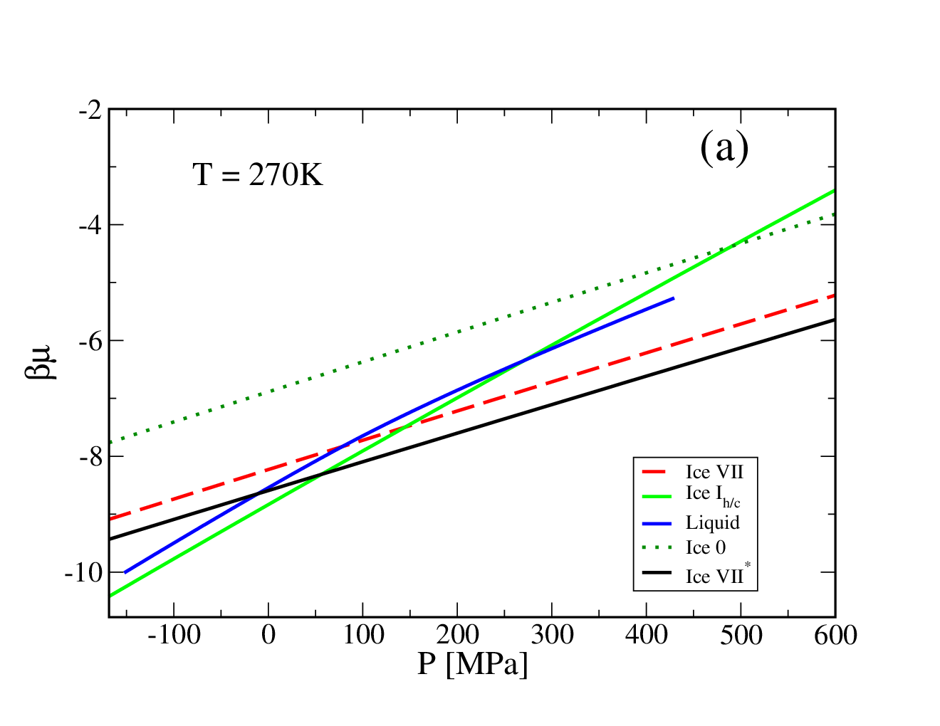
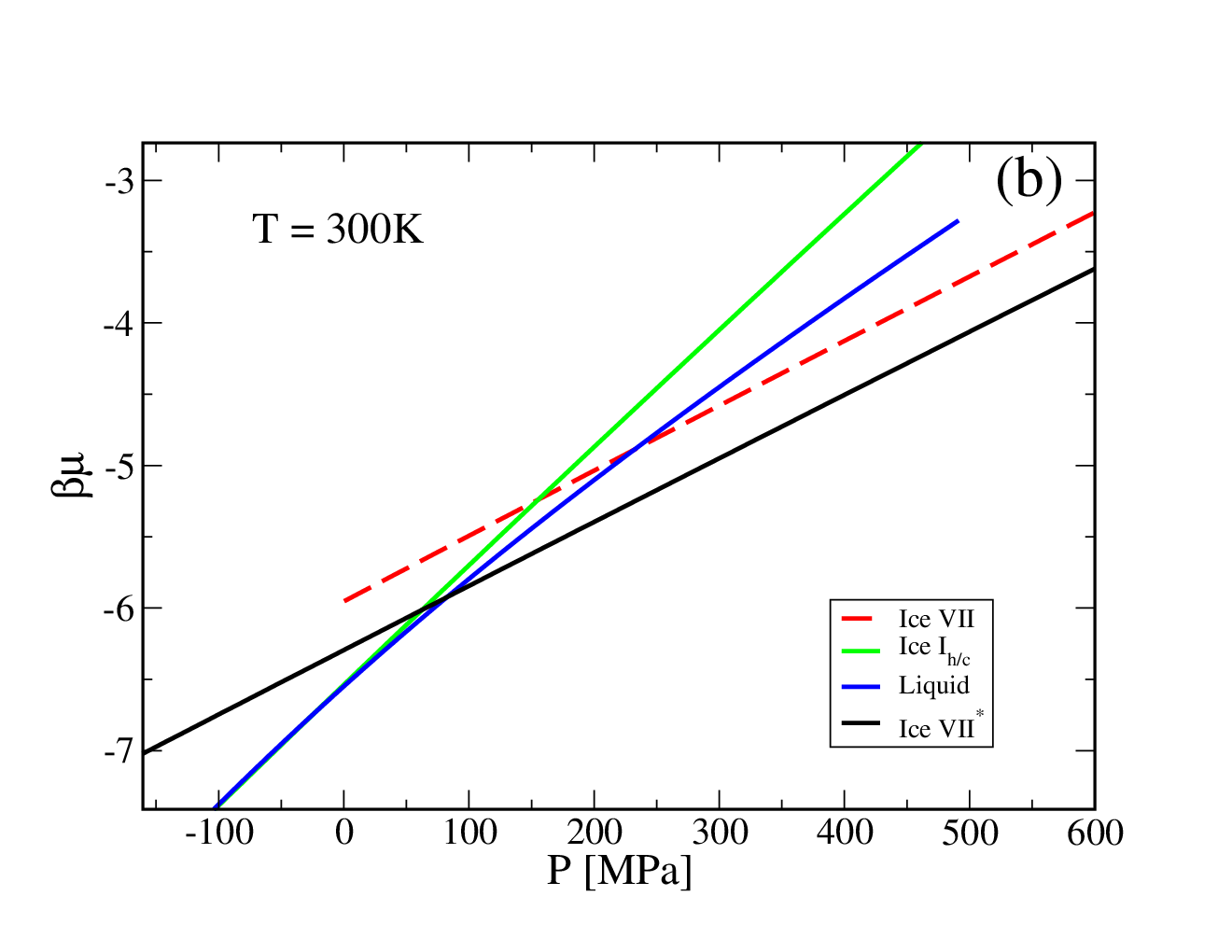
The complete phase diagram is reported in Fig. 5. At low $T$ and low $P$, the most stable crystal structure is the ice I lattice. From our simulations, the cubic (I_c) and hexagonal (I_h) ice structures have the same free energy within our numerical accuracy. At positive pressures, the liquid phase coexisting with ice I is always denser than ice, and as a result, the melting temperature of ice I decreases with increasing $P$. At negative $P$ (near $P=-80$ MPa), the ice I and liquid phases coexist at the same density, and the melting temperature reaches a maximum. We note that we have confirmed the ice I_h/c melting temperature calculated via thermodynamic integration at two separate pressures using direct coexistence simulations, and find good agreement. We note that for the ST2-Ewald model, the melting temperature of I_c at the single pressure of 260 MPa was estimated to be around 274 K, consistent with the present estimate [25].

At high pressure, the main candidate structures are the proton-ordered ice VIII structure, and the proton-disordered ice VII structure. Both structures consist of two interpenetrating I_c lattices (somewhat distorted in the case of proton-ordering), where the oxygen positions form a BCC lattice. According to our free-energy calculations, the disordered ice VII is the more stable one in the region where coexistence with the fluid might occur. However, when trying to confirm the accuracy of our predicted liquid-ice VII coexistences using direct coexistence simulations, we observed crystal growth at temperatures significantly above the melting temperature predicted from free energy calculations. The newly grown parts of the crystal still display the BCC topology of the oxygen atoms, but the crystal shrinks by a few percent in the direction perpendicular to the growth direction, leading to a slight distortion of the lattice, that we refer to in the following as ice VII^∗. As this distortion does not occur in fully disordered ice VII, we attribute the unexpectedly high stability of the ice VII^∗ lattice to the emergence of partial proton ordering, which decreases the crystal free energy. To confirm this, we created a fully regrown ice VII^∗ configuration by alternately melting and regrowing the two halves of an ice VII configuration in an elongated simulation box. When measuring the proton-proton and dipole-dipole correlation functions for both the original ice VII structure and the regrown ice VII^∗, we see only minor changes in the proton-proton correlation function in the region 3 Å$<r<$ 4 Å [see Fig. 6(a)]. In contrast, the dipole-dipole correlation function [see Fig. 6(b)] shows significant additional signal which although weak, extends up to long spatial scales. Using the Frenkel-Ladd method, we calculate the free energy of this configuration (assuming full proton disorder), and find that it is indeed lower than that of the original crystal by $\approx 0.4~k_{B}T$ per particle, confirming that the lower melting temperature observed in our direct coexistence simulations can be attributed to the (slight) change in crystal structure. The difference in free energy mainly results from the lower potential energy of the regrown crystal. We note here that partial proton ordering would reduce the contribution of the residual entropy to the free energy of the crystal, causing us to underestimate the ice VII^∗ free energy. On the other hand, the presence of defects in the system is expected to cause an overestimate in the crystal free energy. It is thus not a priori obvious that this free energy can be used to predict coexistences. Nonetheless, comparing the melting temperature predicted from the free energy and equations of state of the regrown crystal with the melting temperature taken from the direct coexistence simulations, we find good agreement ($T\approx 320K\pm 5K$ at $P=250$ MPa). Calculating the rest of the coexistence lines for this crystal using thermodynamic integration, we observe that ice VII^∗ has a significantly larger stability region than the original ice VII (see Fig. 5).

We note that neither ice VI nor ice 0 are ever the most thermodynamically stable phase in the investigated region. As it may be relevant in future nucleation studies, we include the metastable coexistence line of the liquid with ice 0 in the phase diagram (Fig. 5).

References

- [1] P. G. Debenedetti and H. E. Stanley, Phys. Today 56, 40 (2003).
- [2] P. H. Poole, F. Sciortino, U. Essmann, and H. E. Stanley, Nature 360, 324 (1992).
- [3] F. H. Stillinger and A. Rahman, J. Chem. Phys. 60, 1545 (1974).
- [4] L. Xu, P. Kumar, S. V. Buldyrev, S.-H. Chen, P. H. Poole, F. Sciortino, and H. E. Stanley, Proc. Natl. Acad. Sci. U.S.A. 102, 16558 (2005).
- [5] O. Mishima and H. E. Stanley, Nature 396, 329 (1998).
- [6] A. K. Soper and M. A. Ricci, Phys. Rev. Lett. 84, 2881 (2000).
- [7] Y. Katayama, T. Mizutani, W. Utsumi, O. Shimomura, M. Yamakata, and K.-i. Funakoshi, Nature 403, 170 (2000).
- [8] R. Kurita and H. Tanaka, Science 306, 845 (2004).
- [9] A. Taschin, P. Bartolini, R. Eramo, R. Righini, and R. Torre, Nat. Commun. 4 (2013).
- [10] G. Pallares, M. E. M. Azouzi, M. A. González, J. L. Aragones, J. L. Abascal, C. Valeriani, and F. Caupin, Proc. Natl. Acad. Sci. U.S.A. 111, 7936 (2014).
- [11] K. Amann-Winkel, C. Gainaru, P. H. Handle, M. Seidl, H. Nelson, R. Böhmer, and T. Loerting, Proc. Natl. Acad. Sci. U.S.A. 110, 17720 (2013).
- [12] M. E. M. Azouzi, C. Ramboz, J.-F. Lenain, and F. Caupin, Nature Phys. 9, 38 (2013).
- [13] J. A. Sellberg, C. Huang, T. McQueen, N. Loh, H. Laksmono, D. Schlesinger, R. Sierra, D. Nordlund, C. Hampton, D. Starodub, et al., Nature 510, 381 (2014).
- [14] I. Saika-Voivod, F. Sciortino, and P. H. Poole, Phys. Rev. E 63, 011202 (2001).
- [15] V. V. Vasisht, S. Saw, and S. Sastry, Nat. Phys. 7, 549 (2011).
- [16] C. W. Hsu, J. Largo, F. Sciortino, and F. W. Starr, Proc. Natl. Acad. Sci. U.S.A. 105, 13711 (2008).
- [17] J. L. Abascal and C. Vega, J. Chem. Phys. 133, 234502 (2010).
- [18] F. Smallenburg, L. Filion, and F. Sciortino, Nature Phys. 10, 653 (2014).
- [19] F. W. Starr and F. Sciortino, Soft Matter 10, 9413 (2014).
- [20] E. Jagla, J. Chem. Phys. 111, 8980 (1999).
- [21] G. Franzese, G. Malescio, A. Skibinsky, S. V. Buldyrev, and H. E. Stanley, Nature 409, 692 (2001a).
- [22] L. Xu, S. V. Buldyrev, C. A. Angell, and H. E. Stanley, Phys. Rev. E 74, 031108 (2006).
- [23] P. Gallo and F. Sciortino, Phys. Rev. Lett. 109, 177801 (2012).
- [24] D. T. Limmer and D. Chandler, J. Chem. Phys. 135, 134503 (2011).
- [25] J. C. Palmer, F. Martelli, Y. Liu, R. Car, A. Z. Panagiotopoulos, and P. G. Debenedetti, Nature 510, 385 (2014).
- [26] R. S. Singh and B. Bagchi, J. Chem. Phys. 140, 164503 (2014).
- [27] C. R. C. Buhariwalla, R. K. Bowles, I. Saika-Voivod, F. Sciortino, and P. H. Poole, preprint, arxiv:1501.03115 (2015).
- [28] F. Romano, E. Sanz, and F. Sciortino, J. Chem. Phys. 134, 174502 (pages 8) (2011).
- [29] A preliminary study of the liquid-ice Ih coexistence line for the ST2 model was carried out by A. Rehtanz, A. Geiger, and P.H. Poole; see A. Rehtanz, Ph.D. thesis, Dortmund University (Logos Verlag, Berlin, 2000).
- [30] D. Frenkel and A. J. C. Ladd, J. Chem. Phys 81, 3188 (1984).
- [31] C. Vega, E. Sanz, J. Abascal, and E. Noya, J. Phys.: Condens. Matter 20, 153101 (2008).
- [32] J. Russo, F. Romano, and H. Tanaka, Nature materials 13, 733 (2014).
- [33] D. Quigley, D. Alfè, and B. Slater, J. Chem. Phys. 141, 161102 (2014).
- [34] P. H. Poole, S. R. Becker, F. Sciortino, and F. W. Starr, The Journal of Physical Chemistry B 115, 14176 (2011).
- [35] E. G. Noya, M. M. Conde, and C. Vega, J. Chem. Phys. 129, 104704 (2008).
- [36] B. Smith and D. Frenkel, Understanding molecular simulations (Academic Press, New York, 1996).
- [37] L. Pauling, The Nature of the Chemical Bond (Cornell University Press, Ithaca, New York, 1945).
- [38] B. A. Berg, C. Muguruma, and Y. Okamoto, Phys. Rev. B 75, 092202 (2007).
- [39] P. Virnau and M. Müller, J. Chem. Phys. 120, 10925 (2004).
- [40] F. Sciortino, I. Saika-Voivod, and P. H. Poole, Phys. Chem. Chem. Phys. 13, 19759 (2011).
- [41] N. B. Wilding, Phys. Rev. E 52, 602 (1995).
- [42] A. M. Ferrenberg and D. Landau, Phys. Rev. B 44, 5081 (1991).
- [43] A. Pelissetto and E. Vicari, Phys. Rep. 368, 549 (2002).
- [44] M. J. Cuthbertson and P. H. Poole, Phys. Rev. Lett. 106, 115706 (2011).
- [45] G. Franzese, G. Malescio, A. Skibinsky, S. V. Buldyrev, and H. Stanley, Nature 409, 692 (2001b).
- [46] F. Sciortino, E. La Nave, and P. Tartaglia, Phys. Rev. Lett. 91, 155701 (2003).
- [47] D. Fuentevilla and M. Anisimov, Phys. Rev. Lett. 97, 195702 (2006).
- [48] V. Holten, C. E. Bertrand, M. A. Anisimov, and J. V. Sengers, J. Chem. Phys. 136, 094507 (2012).
- [49] V. Holten, J. C. Palmer, P. H. Poole, P. G. Debenedetti, and M. A. Anisimov, J. Chem. Phys. 140, 104502 (2014).
- [50] F. Smallenburg and F. Sciortino, to be published (2015).