A Linear Network Code Construction for
General Integer Connections Based on
the Constraint Satisfaction Problem
Abstract
The problem of finding network codes for general connections is inherently difficult in capacity constrained networks. Resource minimization for general connections with network coding is further complicated. Existing methods for identifying solutions mainly rely on highly restricted classes of network codes, and are almost all centralized. In this paper, we introduce linear network mixing coefficients for code constructions of general connections that generalize random linear network coding (RLNC) for multicast connections. For such code constructions, we pose the problem of cost minimization for the subgraph involved in the coding solution and relate this minimization to a path-based Constraint Satisfaction Problem (CSP) and an edge-based CSP. While CSPs are NP-complete in general, we present a path-based probabilistic distributed algorithm and an edge-based probabilistic distributed algorithm with almost sure convergence in finite time by applying Communication Free Learning (CFL). Our approach allows fairly general coding across flows, guarantees no greater cost than routing, and shows a possible distributed implementation. Numerical results illustrate the performance improvement of our approach over existing methods.
Index Terms:
network coding, network mixing, general connection, resource optimization, distributed algorithm.I Introduction
The problem of finding network codes in the case of general connections, where each destination can request information from any subset of sources, is intrinsically difficult and little is known about its complexity. In certain special cases, such as multicast connections (where destinations share all of their demands), it suffices to satisfy a Ford-Fulkerson type of min-cut max-flow constraint between all sources to every destination individually. For multicast connections, linear codes suffice [1, 2], and lend themselves to a distributed random construction [3]. While linear codes have been the most widely considered in the literature, linear codes over finite fields may in general not be sufficient for general connections, as shown by [4] using an example from matroid theory.
A matroidal structure for the network coding problem with general connections was conjectured by the late Ralf Kötter (private communication) but, while different aspects of this connection have been investigated in the literature [5, 6, 7, 8, 9, 10, 11], a proof remains elusive, except in special cases. Recently, the problem of scalar-linear coding has been shown to have a matroidal structure [7, 12, 8]. There exists a correspondence between scalar-linearly solvable networks and representable matroids over finite fields, which can be used to obtain some bounds on scalar linear network capacity [13] or the capacity regions of certain classes of networks [14]. More generally, the problem of finding the linear network coding capacity region is equivalent to the characterization of all linear polymatroids [9], whose structure was investigated in [10]. Reference [11] generalized the results of [15], which investigated the connection among index coding, network coding and matroid theory. In [16], polymatroids were used to produce linear code constructions.
Progress in understanding the matroidal structure of the general connection problem has, however, not yet provided simple and useful approaches to generating explicit linear codes. There has been considerable investigation of restricted cases, such as a network with only two sources and two destinations, generally referred to as the two-unicast network [17, 18, 19, 20, 21], but thus far such investigation has yielded only bounds or linear solutions for restricted cases of the two-unicast network. It has been shown in [20] that the two-unicast problem is as hard as the most general network coding problem. Since the difficulty of coding in the case of general connections is in effect an interference cancellation one, approaches relying on interference alignment have naturally been explored [22, 23, 24]. Reference [25] investigated the enumeration, rate region computation and hierarchy of general multi-source multi-sink hyper-edge networks under network coding.
Even when we consider simple scalar network codes, which have scalar coding coefficients, the problem of code construction for general connections remains vexing. The main difficulty lies in cancelling the effect of flows that are coded together even though they are not destined for a common destination. The problem of code construction is further complicated when we seek, for common reasons of network resource management, to limit fully or partially the use of links in the network. For convex cost functions of flows over edges in the graph corresponding to the network, finding a minimum-cost solution is known to be a convex optimization problem in the case of multicast connections (for continuous flows)[26]. However, in the case of general connections, network resource minimization, even when allowing only restricted code constructions, appears difficult.
Among coding approaches for optimizing network use for general connections, we distinguish two types. The first, which we adopt in this paper, is that of mixing, by which we mean coding together flows using random linear network coding (RLNC) [3], originally proposed for multicast connections. The principle is to code together flows as though they were part of a common multicast connection. In this case, no explicit coding coefficients are provided, and decidability is ensured with high probability by RLNC. For example, the mixing approaches in [27] and [28] are both based on mixing variables, each corresponding to a set of flows that can be mixed over an edge. Specifically, in [27], a two-step mixing approach is proposed for network resource minimization of general connections, where flow partition (mixing) and flow rate optimization are considered separately. This separation imposes stronger restrictions on the mixing design in the first step and leads to a limitation on the feasibility region. Reference [28] studies the feasibility of more general mixing designs based on mixing variables of size , where is the number of flows. Reference [28] does not, however, provide an approach for obtaining a specific mixing design. The second type of coding approach is an explicit linear code construction, by which we mean providing specific linear coefficients over some finite field, to be applied to coding flows at different nodes. Often these constructions are simplified by restricting them to be pairwise. For example, in [29] and [30], simple codes over pairs of flows are proposed for network resource minimization of general connections.
Some explicit linear network code construction approaches [29], [30] are distributed, but they allow only pairwise coding. The algorithms of [31] using evolutionary techniques, which are also explicit code constructions, are partially distributed, since the chromosomes can be decomposed into their local contributions, but require information to be fed back from the receivers to all the nodes in the network. In addition, the convergence results for evolutionary techniques are generally scant and do not yield prescriptive constructions. While RLNC for multicast connections is a distributed algorithm, most of the mixing approaches [27], [28] based on it have remained centralized. In [32], we propose new methods for constructing linear network codes for general connections of continuous flows based on mixing to minimize the total network cost. Flow splitting and coding over time are required to achieve the desired performance. The focus in [32] is to apply continuous optimization techniques to obtain continuous flow rates. In [33], we consider linear network code construction for general connections of integer flows based on mixing, and propose an edge-based probabilistic distributed algorithm to minimize the total network cost. This paper extends the results in [33].
Our contribution in this paper is to present new methods for constructing linear network codes in a distributed manner for general connections of integer flows based on mixing.
We introduce linear network mixing coefficients. The number of mixing coefficients grows polynomially with the number of flows. We formally establish the relationship between linear network coding and mixing.
We formulate the minimization of the cost of the subgraph involved in the code construction for general connections of integer flows in terms of the mixing coefficients.
We relate our problem to a path-based Constraint Satisfaction Problem (CSP) and an edge-based CSP. While CSPs are NP-complete in general, we present a path-based probabilistic distributed algorithm and an edge-based probabilistic distributed algorithm with almost sure convergence in finite time by applying Communication Free Learning (CFL), a recent probabilistic distributed solution for CSPs[34]. The path-based distributed algorithm requires more local information than the edge-based distributed algorithm, but converges faster.
We show that our approach guarantees no greater cost than routing or the simplified mixing design in [27]. Numerical results also illustrate the performance improvement of our approach over existing methods.
While our approach, like all other general connection code constructions, is generally suboptimal, it allows more flows to be mixed than is possible with pairwise mixing [29], [30] and with the separate mixing design in [27]. Moreover, in contrast to [27, 28, 32], our approach does not require non-scalar coding over time.
II Problem Setup and Definitions
II-A Network Model
We consider a directed acyclic network with general connections.11 1 The network model we considered in this paper is similar to that in [32] for continuous flows, but here we consider integer flows and edge capacities, and do not allow flow splitting and coding over time. Let denote the directed acyclic graph, where denotes the set of nodes and denotes the set of edges. To simplify notation, we assume there is only one edge from node to node , denoted as edge .22 2 Multiple edges from node to node can be modeled by introducing multiple extra nodes, one on each edge, to transform a multigraph intro a graph. For each node , define the set of incoming neighbors to be and the set of outgoing neighbors to be . Let and denote the in-degree and out-degree of node , respectively. Assume and for all , where is a constant.
Consider a finite field with size . Let denote the set of flows of symbols in finite field to be carried by the network. For each flow , let be its source. We consider integer flows. To simplify notation, we assume unit source rate (i.e., one finite field symbol per second).33 3 A source with a positive integer source rate greater than one can be modeled by multiple sources, each with unit source rate. Let denote the set of sources. We assume different flows do not share a common source node and no source node has any incoming edges. Let denote the set of terminals. Each terminal demands a subset of flows . Assume . Let denote the demands of all the terminals. We assume no terminal has any outgoing edges.
As we consider integer flows, we assume unit edge capacity (i.e., one finite field symbol per second).44 4 An edge with a positive integer edge capacity greater than one can be equivalently converted to multiple edges, each with unit edge capacity. Let denote whether edge is in the subgraph involved in the code construction in a sense we shall make precise later.55 5 There is either no flow or a unit rate of (coded) flow through each edge. Under the unit source rate and edge capacity assumptions, we shall see that there is one global coding (mixing) vector for each edge. We assume a cost is incurred on an edge when information is transmitted through the edge and let denote the cost function for edge . We assume is non-decreasing in . We are interested in the problem of finding linear network coding designs and minimizing the network cost for general connections under those designs.
II-B Scalar Time-Invariant Linear Network Coding
In linear network coding, a linear combination over of the symbols in from the incoming edges can be transmitted through the shared edge . The coefficients used to form this linear combination are referred to as local coding coefficients. Specifically, let denote the local coding coefficient corresponding to edge and edge . Denote . Then, for linear network coding, using local coding coefficients, the symbol through edge can be expressed as
| (1) |
This is illustrated in Fig. 1.
Starting from the sources, we transmit source symbols , and then, at intermediate nodes, we perform only linear operations over on the symbols from incoming edges. Thus, the symbol of each edge can be expressed as a linear combination over of the source symbols . Let denote the coefficient of flow in the linear combination for edge . This is referred to as the global coding coefficient of flow and edge . Let denote coefficients corresponding to this linear combination for edge . This is referred to as the global coding vector of edge . Here, represents the set of global coding vectors, the cardinality of which is . Then, using global coding vectors, the symbol through edge can also be expressed as
| (2) |
This is illustrated in Fig. 1.

In this paper, we consider scalar time-invariant linear network coding. In other words, and are both scalars, and do not change over time. Let denote the vector with the -th element being 1 and all the other elements being 0. For decodability to hold at all the terminals, the global coding vectors at all edges must satisfy the following feasibility condition for scalar linear network coding.
Definition 1 (Feasibility of Scalar Linear Network Coding)
For a network and a set of flows with sources and terminals , a linear network code is called feasible if the following three conditions are satisfied: 1) for source edge , where and ; 2) for edge not outgoing from a source, where and ; 3) , where and .
Note that when using scalar linear network coding, for each terminal, extraneous flows are allowed to be mixed with the desired flows on the paths to the terminal, as the extraneous flows can be cancelled at intermediate nodes or at the terminal.
II-C Scalar Time-Invariant Linear Network Mixing
As mentioned in Section I, to facilitate distributed linear network code designs for general connections using the mixing concept (without requiring the specific values of local or global coding coefficients in the designs), we introduce local and global mixing variables. Later, we shall see that distributed linear network mixing designs in terms of these mixing coefficients are much easier. Specifically, we introduce the local mixing coefficient corresponding to edge and edge , which relates to the local coding coefficient . Denote . indicates that symbol of edge is allowed (under our construction) to contribute to the linear combination over forming symbol in (1) and otherwise. Thus, if , we have ; if , we can further determine how symbol contributes to the linear combination forming symbol by choosing (note that can be zero when ).
Similarly, we introduce the global mixing coefficient of flow and edge , which relates to the global coding coefficient . indicates that flow is allowed (under our construction) to be mixed (coded) with other flows, i.e., symbol is allowed to contribute to the linear combination over forming symbol in (2), and otherwise. Thus, if , we have ; if , we can further determine how symbol contributes to the linear combination forming symbol (note that can be zero when ). Then, we introduce the global mixing vector for edge , which relates to the global coding vector . Here, represents the set of global mixing vectors, the cardinality of which is .
We consider scalar time-invariant linear network mixing. In other words, and are both scalars, and and do not change over time.
Global mixing vectors provide a natural way of speaking of flows as possibly coded or not without knowledge of the specific values of global coding vectors. Intuitively, global mixing vectors can be regarded as a limited representation of global coding vectors. Given network mixing vectors, it may not be sufficient to tell whether a certain symbol can be decoded or not. Thus, using the network mixing representation, the extraneous flows, when mixed with the desired flows on the paths to each terminal, are not guaranteed to be cancelled at the terminal. For decodability to hold at all the terminals, the global mixing vectors at all edges must satisfy the following feasibility condition for scalar linear network mixing.
Definition 2 (Feasibility of Scalar Linear Network Mixing)
For a network and a set of flows with sources and terminals , a linear network mixing design is called feasible if the following three conditions are satisfied: 1) for source edge , where and ; 2) for edge not outgoing from a source, where and ;66 6 Note that denotes the “or” operator (logical disjunction). 3) , where , , .
Note that Condition 3) in Definition 2 ensures that for each terminal, the extraneous flows are not mixed with the desired flows on the paths to the terminal. In other words, linear mixing allows only mixing at intermediate nodes. This is not as general as using linear network coding, which allows mixing and canceling (i.e., removing one or multiple flows from a mixing of flows) at intermediate nodes.
Given a feasible linear network mixing design, one of the ways to implement mixing when is large is to use random linear network coding (RLNC)[3, 27], as discussed in the introduction. In particular, when , can be randomly, uniformly, and independently chosen in using RLNC; when , has to be chosen to be 0.
III Mixing Problem Formulation
In this section, we formulate the problem of selecting mixing coefficients and to minimize the cost of the subgraph involved in the coding solution, i.e., the set of edges used in delivering the flows.
In the following formulation, indicates whether edge is involved in delivering flows, and indicates whether edge is involved in delivering flow to terminal .
Problem 1 (Mixing)
| (3) | ||||
| (4) | ||||
| (5) | ||||
| (6) | ||||
| (7) | ||||
| (8) | ||||
| (9) | ||||
| (10) | ||||
| (11) | ||||
| (12) |
where
| (13) |
Here, and .77 7 Note that the optimal value in Problem 7 is a function of , , and , which are assumed to be fixed. Here, we write as a function of only to emphasize the impact of on , which is helpful when considering demand set expansion in Problem 2.
Consider a feasible solution , , and to Problem 7. By (6) and (8), we know that for all and , all the edges in form one flow path (i.e., a set of ordered edges such that ) from source to terminal . In addition, combining (3) and (7), we have an equivalent constraint purely in terms of , i.e.,
| (14) |
From this, we know that for all , and , the two flow paths from sources and to terminal are edge-disjoint. Finally, the feasibility constraints in (10), (11) and (12) together with (4) and (5) set other requirements on flow paths (i.e., ) via the constraint in (9). Therefore, a feasible solution to Problem 7 corresponds to a set of flow paths satisfying certain requirements, as illustrated above. These interpretations can be understood from the following example.
Example 1 (Illustration of Problem 7)
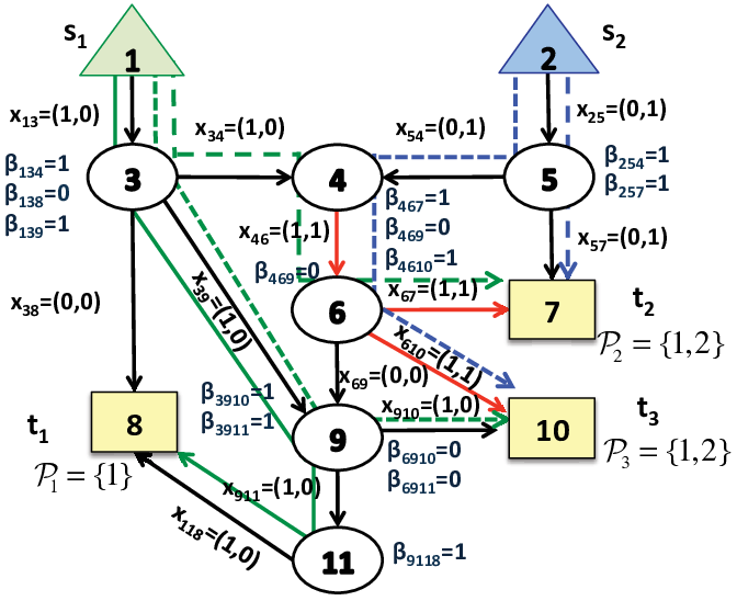
As illustrated in Fig. 2, we consider a network with , , , , , and for all . Problem 7 for the network in Fig. 2 has two feasible solutions of network costs 11 and 12, as illustrated in Fig. 2 (a) and Fig. 2 (b), respectively. Specifically, the two feasible solutions share the same flow paths from sources and to terminals and , i.e., flow paths , , , . Notice that the two feasible solutions have different flow paths from source to terminal , i.e., flow path for the feasible solution in Fig. 2 (a) and flow path for the feasible solution in Fig. 2 (b). The optimal solution is the one illustrated in Fig. 2 (a) and the optimal network cost is 11.

We now illustrate the complexity of Problem 7. The number of variables in is . The number of variables in is smaller than or equal to . The numbers of variables in and are and , respectively. Therefore, the total number of variables in Problem 7 is smaller than or equal to , i.e., polynomial in , and . Problem 7 is a binary optimization problem, and does not appear to have a ready solution.
Remark 1 (Problem 7 for Multicast)
When for all (i.e., multicast), the constraint in (12) does not exist, and the constraint in (9) is always satisfied by choosing for all and choosing accordingly by (10) and (11). Therefore, Problem 7 for general connections reduces to the conventional minimum-cost scalar time-invariant linear network code design problem for the multicast case. The complexity of the optimization for the multicast case is much lower than that for the general case. This is because in the optimization for the multicast case, variables and do not appear, and the constraints in (4), (5), (9), (10), (11) and (12) can be removed.
In the following, we show that a feasible linear network code can be obtained using a feasible solution to Problem 7 (e.g., using RLNC[3]), as illustrated in Section II-C.
Theorem 1
Suppose Problem 7 is feasible. Then, for each feasible and , there exists a feasible linear network code design and with a field size to deliver the desired flows to each terminal.
Proof:
Please refer to Appendix A. ∎
Next, the minimum network cost of Problem 7 is no greater than the minimum costs of the two-step mixing approach for general connections in [27] and routing for integer flows, owing to the following reasons. Problem 7 with for all , instead of (5), is equivalent to the minimum-cost flow rate control problem in the second step of the two-step mixing approach for general connections in [27]. Problem 7 with an extra constraint for all is equivalent to the minimum-cost routing problem. Fig. 2 illustrates a feasible solution to Problem 7 that cannot be obtained by the two-step mixing approach [27] or routing. In this example, the minimum network cost of Problem 7 is smaller than those of the two-step mixing approach[27] and routing (which can be treated as infinity).
When for all and (e.g., multiple unicasts), Problem 7 for general connections reduces to the minimum-cost routing problem and cannot take advantage of the network coding gain. This is because using the network mixing representation, for decodability to hold, the extraneous flows of each terminal are not allowed to be mixed with the terminal’s desired flows on the path to this terminal, thus limiting the network coding gain. To address this limitation, we now formulate Problem 2, which allows the expansion of the demand sets and the optimization over the expansions to increase the opportunity for mixing flows to different terminals. Let denote the expanded demand set, which satisfies . Let denote the expanded demand sets of all the terminals.
Problem 2 (Mixing with Demand Set Expansion)
| (15) | ||||
| (16) |
where is the optimal value to Problem 7 for .
The network coding gain improvement of Problem 2 can be easily understood from the case of two unicasts over the butterfly network, as illustrated in Fig. 3. By Theorem 1, we can easily show the following result.
Corollary 1
Suppose Problem 2 is feasible. Then, for each feasible solution, there exists a feasible linear network code design with a field size to deliver the desired flows to each terminal.

IV Centralized Algorithm
In this section, we develop a centralized algorithm to solve Problem 7, based on the concept of edge-disjoint flow paths discussed before. The centralized algorithm is conducted at a central node which is aware of global network information.
For all and , let denote the number of flow paths from source to terminal . For Problem 7 to be feasible, assume . As illustrated in Section III, obtaining a feasible solution to Problem 7 is equivalent to selecting a set of flow paths satisfying certain requirements. Thus, we introduce flow path selection variables to indicate the flow paths selected for information transmission. Let denote the flow path selection variable for source and terminal (i.e., the index of the selected flow path from source to terminal ). Denote the flow path selection variables as . In the following, we express variables and in terms of . To satisfy (6) and (8), we require to take only one value from . Let denote the selected flow path (i.e., the set of edges on the selected flow path) from source to terminal . To satisfy (3) and (7) (or equivalently (14)), we require that the flow paths from sources to terminal are edge-disjoint, i.e.,
| (17) |
Then, variables can be expressed in terms of variables as follows:
| (18) |
By (7) and the monotonicity of , variables can be chosen based on and expressed implicitly in terms of variables as follows:
| (19) |
In addition, to satisfy (4), (5), (9) and (11), can be chosen based on and expressed implicitly in terms of variables as follows:
| (20) |
Then, based on , (10) and (11), can be determined in topological order88 8 A topological order of a directed graph is an ordering of its nodes such that for every directed edge from node to node , comes before in the ordering. Such an order exists for the edges of any directed graph that is acyclic. and expressed implicitly in terms of variables . Finally, to satisfy (12), we require
| (21) |
Based on the above relationship between the flow path selection variables and the variables of Problem 7, we now describe the procedure of the centralized algorithm, i.e., Algorithm 1, which obtains the feasible flow paths of the minimum network cost.
Note that Constraints (6) and (8) are guaranteed in Step 1 and Step 8; Constraints (3) and (7) are guaranteed in Step 2 and Step 7; Constraints (4), (5), (9) are guaranteed in Step 9; Constraints (10) and (11) are guaranteed in Step 10; and Constraint (12) is considered in Steps 11–15. Therefore, we can see that the optimization to Problem 7 can be obtained by Algorithm 1.
V Probabilistic Distributed Algorithms
In this section, using recent results for CSP [34], we develop two probabilistic distributed algorithms to solve Problem 7.
V-A Background on Decentralized CSP
We review some existing results on CSP in [34].
Definition 3 (Constraint Satisfaction Problem)
[34] A CSP consists of variables and clauses . Each variable takes values in a finite set , i.e., for all . Let . Each clause is a function , where for an assignment of variables , if clause is satisfied and otherwise. An assignment is a solution to the CSP if and only if all clauses are simultaneously satisfied
| (22) |
To solve a CSP in a distributed way, clause participation is introduced in [34]. Let . For each variable , let denote the set of clause indices in which it participates, i.e., . Thus, we can rewrite the left hand side of (22) in a way that focuses on the satisfaction of each variable, i.e., . This form enables us to solve CSPs in a distributed iterative way by locally evaluating the clauses in and then updating .
CSPs are in general NP-complete and most effective CSP solvers are designed for centralized problems. The CFL algorithm [34, Algorithm 1], summarized in Algorithm 2, is a distributed iterative algorithm which can find a satisfying assignment to a CSP almost surely in finite time [34, Corollary 2]. Note that Algorithm 2 keeps a probability distribution over all possible values of each variable. The value of each variable is selected from this distribution. For each variable, if all the clauses in which a variable participates are satisfied with its current value, the associated probability distribution is updated to ensure that the variable value remains unchanged; if at least one clause is unsatisfied, the probability distribution evolves by interpolating between it and a distribution that is uniform on all values except the one that is currently generating dissatisfaction. Therefore, if all variables are simultaneously satisfied in all clauses, the same assignment of values will be reselected indefinitely with probability 1.
V-B Path-based Probabilistic Distributed Algorithm
In this part, we develop a path-based probabilistic distributed algorithm to solve Problem 7, using recent results in [34]. This distributed algorithm is based on the concept of edge-disjoint flow paths discussed before. It can be viewed as a distributed version of the path-based centralized algorithm, i.e., Algorithm 1. For all , and , this algorithm requires each node on the -th flow path from source to terminal to know its neighboring edge on this flow path. Note that it is not necessary for each node on the -th flow path to be aware of other edges on the -th flow path.
First, we construct a path-based CSP corresponding to the feasibility problem obtained from Problem 7. Treat as the variables of the path-based CSP, where denotes the index of the selected flow path from source to terminal . As illustrated in Section IV, the constraints of in (6) and (8) for Problem 7 can be taken into account by choosing , for all and . The constraints in (3) and (7) (or equivalently (14)) can be replaced by the constraint of in (17) for the path-based CSP. Variables and can be determined for given via (18), (20), (10) and (11). Thus, the last constraint in (12) of Problem 7 can be replaced by the constraint of for the path-based CSP in (21). Therefore, we can write the clause for as follows:
| (23) |
We thus have the following proposition.99 9 Note that the clauses of the path-based CSP cannot be further partitioned, as all the variables are coupled in general.
Proposition 1 (Path-based CSP)
Now, we present a path-based distributed probabilistic algorithm, i.e., Algorithm 3, to obtain a feasible solution to the path-based CSP using CFL [34, Algorithm 1]. Based on the convergence result of CFL [34, Corollary 2], we know that Algorithm 3 can find a feasible solution to Problem 7 in almost surely finite time. Fig. 4 illustrates the convergence of Algorithm 3. From Fig. 4, we can see that Algorithm 3 converges to a feasible solution (i.e., the feasible solution illustrated in Fig. 2 (a)) to Problem 7 for the network in Fig. 2 quite quickly (within 35 iterations). This feasible solution corresponds to flow paths , , , and . The network cost of this feasible solution is 11.
Relying on Algorithm 3, we present a path-based distributed probabilistic algorithm, Algorithm 4, to obtain the optimal solution to Problem 7 among multiple feasible solutions obtained by Algorithm 3.1010 10 In Step 3 of Algorithm 4, the path-based CFL is run for a sufficiently long time. Step 6 of Algorithm 4 can be implemented with a master node obtaining the network cost of the path-based CFL from all nodes or with all nodes computing the average network cost of the path-based CFL locally via a gossip algorithm. Since Algorithm 3 can find any feasible solution to Problem 7 with positive probability, almost surely as , where denotes the minimum network cost obtained by the first path-based CFLs. Fig. 5 illustrates the convergence of Algorithm 4. From Fig. 5, we can see that Algorithm 4 obtains the optimal network cost 11 to Problem 7 for the network in Fig. 2 quite quickly (within 5 iterations).


V-C Edge-based Probabilistic Distributed Algorithm
In this part, we develop an edge-based probabilistic distributed algorithm to solve Problem 7, using recent results in [34]. Compared with the path-based distributed algorithm in Section V-C, this edge-based distributed algorithm does not require any path information.
Obtaining a feasible solution to Problem 7 can be directly treated as a CSP[34]. Specifically, and can be treated as the variables and the finite set of the CSP. Constraints (7)-(12) can be treated as the clauses of the CSP. While CSPs are in general NP-complete, several centralized CSP solvers (see references in [34]) and the distributed CSP solver proposed in [34] can be applied to solve this (naïve) CSP. However, the direct application of the distributed CSP solver in [34] leads to high complexity owing to the large constraint set. In this part, by exploring the features of the constraints in Problem 7, we obtain a different CSP and present a probabilistic distributed solution with a significantly reduced number of clauses.
First, we construct a new problem, which we show to be a CSP. This new problem is better suited than the original problem to being treated using a probabilistic distributed algorithm based on the distributed CSP solver presented in [34]. Combining (3) and (7), we have an equivalent constraint purely in terms of , i.e., (14). In addition, from (11), we have an equivalent constraint purely in terms of , i.e.,
| (24) |
Therefore, we can solve only for variables and in a distributed way, as can be obtained directly from feasible by choosing according to (3) and (7), and can be obtained from feasible by (10) and (11). We group all the local variables for each edge and introduce the vector variable , where , and . We also write , where . We now consider a new CSP, different from the naïve one that would be directly obtained from Problem 7. We treat and as the variable and the finite set for edge of the CSP. We write the clauses for as follows:
| (25) | ||||
| (26) |
where . Note that the local constraints in (4), (6), (9), (10), (12) and (14) (i.e., (3) and (7)) are considered in the finite set of the CSP with respect to each edge . On the other hand, the non-local constraints in (8) and (24) are considered in clauses in (25) and in (26), respectively. We thus have the following proposition.
Proposition 2 (Edge-based CSP)
Note that the number of variables () and the number of clauses () of the new CSP are much smaller than the number of variables () and the number of clauses () of the naïve CSP directly obtained from Problem 7. This feature will favor the complexity reduction of a distributed solution based on the distributed CSP solver in [34].
Next, we construct the clause partition. The set of clauses in which variable participates is
| (27) |
Then, the focus can be on the satisfaction of each variable , i.e., the satisfaction of each set of clauses . Now, the new CSP can be solved using the distributed iterative CFL algorithm [34, Algorithm 1]. Specifically, each edge realizes a random variable selecting . Allow message passing on between adjacent nodes to evaluate the related clauses. Based on whether the clauses in (27) are satisfied or not, the distribution of the random variable of each edge is updated. The details are summarized in Algorithm 5, which obtains a feasible solution to the edge-based CSP using CFL [34, Algorithm 1]. Based on the convergence result of CFL [34, Corollary 2], we know that Algorithm 5 can find a feasible solution to Problem 7 in almost surely finite time. Fig. 6 illustrates the convergence of Algorithm 5. From Fig. 6, we can see that Algorithm 5 converges to a feasible solution to Problem 7 for the network in Fig. 2 within 5000 iterations. This feasible solution is the same as the one shown in Fig. 4, with network cost 11.


Relying on Algorithm 5, we present an edge-based distributed probabilistic algorithm, Algorithm 6, to solve Problem 7.1111 11 Note that Step 3 and Step 6 of Algorithm 6 can be implemented in similar ways to those in Algorithm 4. Since Algorithm 5 can find any feasible solution to Problem 7 with positive probability, almost surely as , where denotes the smallest network cost obtained by the first edge-based CFLs. Fig. 7 illustrates the convergence of Algorithm 6. From Fig. 7, we can see that Algorithm 6 obtains the optimal network cost 11 to Problem 7 for the network in Fig. 2 quite quickly (within 5 iterations).
V-D Comparison
In this part, we compare the path-based and edge-based distributed algorithms. In obtaining a feasible solution to Problem 7, the path-based CFL, i.e., Algorithm 3 and the edge-based CFL, i.e., Algorithm 5 both base on CFL [34, Algorithm 1]. The convergence result of CFL [34, Corollary 2] guarantee that Algorithm 3 and Algorithm 5 both converge to feasible solutions to Problem 7 almost surely in finite time. However, Algorithm 3 converges much faster than Algorithm 5 in our simulations. This is expected, as Algorithm 3 solves a path-based CSP, while Algorithm 5 solves an edge-based CSP. The number of variables and the number of possible values for each variable for the path-based CSP are much smaller than those for the edge-based CSP. The difference in the convergence rates of Algorithm 3 and Algorithm 5 can be seen by comparing Fig. 4 and Fig. 6. On the other hand, Algorithm 3 requires more local information than Algorithm 5. In particular, Algorithm 3 requires all the nodes on one path from a source node to a terminal node to be aware of their neighboring nodes on the path (not all the nodes on the path). Algorithm 5 instead only requires each node to be aware of its neighboring nodes.
In obtaining an optimal solution to Problem 7 among multiple feasible solutions, the path-based distributed algorithm, i.e., Algorithm 4 and the edge-based distributed algorithm, i.e., Algorithm 6 base on the path-based CFL, i.e., Algorithm 3 and the edge-based CFL, i.e., Algorithm 5, respectively, in the same way. Therefore, Algorithm 4 and Algorithm 6 share similar convergence properties. This can be illustrated in Fig. 5 and Fig. 7.
VI Numerical Illustration
In this section, we numerically illustrate the performance of the proposed optimal solutions to Problems 7 and 2 using mixing only with the two-step mixing approach in [27] and optimal routing for general connections of integer flows.
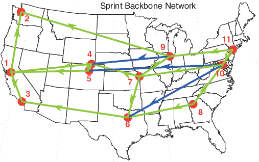
In the simulation, we consider the Sprint backbone network[35] as illustrated in Fig. 8. We choose sources and terminals . The edge directions are chosen to permit connections and help illustrate network coding gain. The green edges have edge cost 1, while the blue edges have edge cost 10 or 20. The edge costs are chosen to make the network coding advantage exist at least for some connection requests[31]. Note that network coding gain takes effect only if transmitting coded information requires a lower network cost than routing. We consider 1000 random realizations of demand sets. For each realization, a pair or triplet of terminals (i.e., ) are selected from uniformly at random, and each selected terminal randomly, uniformly, independently demands a source out of the two sources in . In addition, each selected terminal randomly chooses to demand the other source or not according to a Bernoulli distribution with probability of selecting a second source, where . Thus, represents the expected number of sources selected by each terminal (i.e., ). Note that indicates multicast, and results in unicast connections. In this way, general connections are randomly generated with controlling the average size of the intersections of the demand sets by different terminals.
VI-A Network Cost
| T=2 | T=3 | |||
|---|---|---|---|---|
| q=1.2 | q=1.8 | q=1.2 | q=1.8 | |
| Problem 2 | 7.49 | 12.70 | 12.82 | 20.79 |
| Problem 1 | 8.99 | 13.80 | 16.96 | 23.20 |
| Two-step Mixing[27] | 8.99 | 13.80 | 17.24 | 24.94 |
| Routing | 9.36 | 18.68 | 17.25 | 32.34 |
Table. I illustrates the average optimal network cost (averaged over 1000 random realizations) for different and . Note that the optimal network costs of Problems 7 and 2 are obtained by the centralized algorithm, i.e., Algorithm 1. We can observe that the average optimal network costs of all the schemes increase with increases of or , i.e., the increase of network load. The average network costs of the optimal solutions to Problems 7 and 2 are lower than the optimal routing, with average cost reductions up to and , respectively. The average cost reductions are due to the network coding gain exploited by Problems 7 and 2. Specifically, edge can serve as the coding edge for the butterfly subnetwork consisting of nodes 6, 7, 8, 9, 10 and 11, and edges and can serve as the coding edge for the butterfly subnetwork consisting of nodes 1, 2, 3, 4, 6, 7 and 9, in the Sprint backbone network in Fig. 8. The network coding gain increases as or increases. This is because, using network coding, edges can be used more efficiently in the case of high network load.
In addition, the average network costs of the optimal solutions to Problems 7 and 2 are lower than the two-step mixing approach, with average cost reductions up to and , respectively. The average cost reductions are due to the extra network coding gain (achieved through mixing) exploited by Problems 7 and 2. Specifically, given the demand sets of all the terminals, mixing or not in the two-step mixing approach (determined in the first step, separately from the second flow rate control step) is restricted by all the physical paths, while mixing or not in Problems 7 and 2 (determined jointly with flow rate control) is only restricted by the actual paths that each flow will take, which is also illustrated in the example in Fig. 2. Note that the average network cost of Problem 7 is lower than the two-step mixing when . The average cost reductions of the optimal solutions to Problems 7 and 2 increase as increases, as there are more physical paths to terminals restricting network coding (mixing) in the two-step mixing approach.
On the other hand, the average network cost of the optimal solution to Problem 2 is lower than that of the optimal solution to Problem 7, with average cost reduction up to , illustrating the consequence of Lemma 1. For a given , the performance gain of Problem 2 over Problem 7 decreases as increases, since the difference between the feasibility regions of the two problems reduces with the increase of . Note that when (i.e., multicast), the two problems (feasibility regions) are the same. However, for a given , the performance gain of Problem 2 over Problem 7 increases as increases, since the difference between the feasibility regions of the two problems increases with the increase of .
VI-B Convergence
We illustrate the convergence performance of own distributed Algorithm 4. Consider , , , , , and . In this case, the optimal network costs of Problem 2, Problem 7, the two-step mixing approach and routing are 10, 28, 28, 28, respectively. The optimal network mixing solution to Problem 2 is achieved through the demand set expansion, i.e., . The expanded demand set corresponds to multicast, where the network coding gain is achieved. The optimal mixing (coding) solutions with cost 10 corresponds to flow paths , (), and . There is no network mixing (coding) solution to Problem 7 and the two-step mixing approach. There are three optimal routing solutions of cost 28, which are also optimal (feasible but non-coding) solutions for Problem 7 and the two-step mixing approach. The first one corresponds to flow paths , and . The second one corresponds to flow paths , and . The third one corresponds to flow paths , and . In the following, we illustrate the convergence for the path-based and edge-based distributed algorithms for Problem 2 (at ), respectively.
VI-B1 Path-based Probabilistic Distributed Algorithm


Fig. 9 illustrates the convergence of Algorithm 3 (i.e., Step 3 in Algorithm 4). From Fig. 9, we can see that Algorithm 3 converges to a feasible solution to Problem 2 quite quickly (within 25 iterations). This feasible solution corresponds to flow paths , , and . The network cost of this feasible solution is 10, i.e., the optimal network cost to Problem 2. Fig. 10 illustrates the convergence of Algorithm 4 for one instance. We can see that there exist multiple feasible mixing solutions to Problem 2, which are of different network costs, and running Algorithm 3 for multiple times can result in different feasible solutions. Thus, the minimum network cost may decrease as the number of iterations increases. Algorithm 4 obtains the optimal network cost 10 to Problem 2 quite quickly (within 100 iterations). Fig. 11 illustrates the average convergence of Algorithm 4 over 1000 instances. We can see that on average, within 100 iterations, the minimum network cost under Algorithm 4 converges to 10, which is the optimal network cost to Problem 2 obtained by the centralized algorithm in Algorithm 1.
VI-B2 Edge-based Probabilistic Distributed Algorithm


Fig. 12 illustrates the convergence of Algorithm 5 (i.e., Step 3 in Algorithm 6). From Fig. 12, we can see that Algorithm 5 converges to a feasible solution to Problem 2 within 8000 iterations. This feasible solution is the same as the one shown in Fig. 9, with network cost 10. By comparing Fig. 12 with Fig. 9, we can see that Algorithm 5 converges much more slowly than Algorithm 3. Fig. 13 illustrates the convergence of Algorithm 6. We can see that there exist for Problem 2, multiple feasible mixing solutions which have different network costs, and running Algorithm 5 for multiple times can result in different feasible solutions. Thus, the minimum network cost may decrease as the number of iterations increases. Algorithm 6 obtains the optimal network cost 10 to Problem 2 within 100 iterations. Fig. 14 illustrates the average convergence of Algorithm 6 over 1000 instances. We can see that on average, within 300 iterations, the minimum network cost under Algorithm 6 converges to 10, which is the optimal network cost to Problem 2 obtained by the centralized algorithm in Algorithm 1. By comparing Fig. 14 with Fig. 11, we can see that Algorithm 6 converges much more slowly than Algorithm 4.
VII Conclusion and Future Work
In this paper, we introduce linear network mixing coefficients for code constructions of general integer connections. For such code constructions, we pose the problem of cost minimization for the subgraph involved in the coding solution, and relate this minimization to a path-based CSP and an edge-based CSP, respectively. We present a path-based probabilistic distributed algorithm and an edge-based probabilistic distributed algorithm with almost sure convergence in finite time by applying CFL. Our approach allows fairly general coding across flows, guarantees no greater cost than routing, and demonstrates a possible distributed implementation. Numerical results illustrate the performance improvement of our approach over existing methods.
This paper opens up several directions for future research. For instance, the proposed optimization-based linear network code construction for general integer connections can be extended to design route finding protocols of superior performance for general connections. In addition, a possible direction for future research is to design dynamic approaches not only to build new subgraphs, but also to update them as they evolve, so as to reflect changes in topologies for varying networks, as occur in such settings as peer-to-peer (P2P) networks. Another interesting extension of the proposed approach to content-centric cache-enabled networks is to incorporate cache placement (which creates new sources) into the cost minimization for the subgraph involved in the coding solution in this work. Finally, the proposed approach for wireline networks can also be generalized to wireless networks by considering hyper edges to model broadcast links.
References
- [1] R. Koetter and M. Médard, “Beyond routing: an algebraic approach to network coding,” in INFOCOM 2002. Twenty-First Annual Joint Conference of the IEEE Computer and Communications Societies. Proceedings. IEEE, vol. 1, October 2002, pp. 122–130 vol.1.
- [2] S.-Y. Li, R. Yeung, and N. Cai, “Linear network coding,” Information Theory, IEEE Transactions on, vol. 49, no. 2, pp. 371–381, February 2003.
- [3] T. Ho, M. Médard, R. Koetter, D. Karger, M. Effros, J. Shi, and B. Leong, “A random linear network coding approach to multicast,” Information Theory, IEEE Transactions on, vol. 52, no. 10, pp. 4413–4430, October 2006.
- [4] R. Dougherty, C. Freiling, and K. Zeger, “Insufficiency of linear coding in network information flow,” in Information Theory, 2005. ISIT 2005. Proceedings. International Symposium on, September 2005, pp. 264–267.
- [5] S. El Rouayheb, A. Sprintson, and C. Georghiades, “A new construction method for networks from matroids,” in Information Theory, 2009. ISIT 2009. IEEE International Symposium on, June 2009, pp. 2872–2876.
- [6] Q. Sun, S. T. Ho, and S.-Y. Li, “On network matroids and linear network codes,” in Information Theory, 2008. ISIT 2008. IEEE International Symposium on, July 2008, pp. 1833–1837.
- [7] R. Dougherty, C. Freiling, and K. Zeger, “Matroidal networks,” in Allerton Conference on Communication, Control, and Computing, September 2007.
- [8] A. Kim and M. Médard, “Scalar-linear solvability of matroidal networks associated with representable matroids,” in Turbo Codes and Iterative Information Processing (ISTC), 2010 6th International Symposium on, Sep 2010, pp. 452–456.
- [9] X. Yan, R. Yeung, and Z. Zhang, “The capacity region for multi-source multi-sink network coding,” in Information Theory, 2007. ISIT 2007. IEEE International Symposium on, June 2007, pp. 116–120.
- [10] T. Chan, A. Grant, and D. Pfluger, “Truncation technique for characterizing linear polymatroids,” Information Theory, IEEE Transactions on, vol. 57, no. 10, pp. 6364–6378, 2011.
- [11] V. T. Muralidharan and B. S. Rajan, “Linear index coding and representable discrete polymatroids,” in Information Theory (ISIT), 2014 IEEE International Symposium on, June 2014, pp. 486–490.
- [12] R. Dougherty, C. Freiling, and K. Zeger, “Networks, matroids, and non-shannon information inequalities,” Information Theory, IEEE Transactions on, vol. 53, no. 6, pp. 1949–1969, June 2007.
- [13] A. Kim and M. Médard, “Computing bounds on network capacity regions as a polytope reconstruction problem,” in Information Theory Proceedings (ISIT), 2011 IEEE International Symposium on, July 2011, pp. 588–592.
- [14] R. Dougherty, C. Freiling, and K. Zeger, “Achievable rate regions for network coding,” in Information Theory and Applications Workshop (ITA), 2012, February 2012, pp. 160–167.
- [15] S. El Rouayheb, A. Sprintson, and C. Georghiades, “On the index coding problem and its relation to network coding and matroid theory,” Information Theory, IEEE Transactions on, vol. 56, no. 7, pp. 3187–3195, 2010.
- [16] A. Salimi, M. Médard, and S. Cui, “On the representability of integer polymatroids: Applications in linear code construction,” in 53rd Annual Allerton Conference on Communication, Control, and Computing, Monticello, IL, USA, September 2015.
- [17] W. Zeng, V. R. Cadambe, and M. Médard, “An edge reduction lemma for linear network coding and an application to two-unicast networks,” in Communication, Control, and Computing (Allerton), 2012 50th Annual Allerton Conference on. IEEE, 2012, pp. 509–516.
- [18] C.-C. Wang and N. Shroff, “Pairwise intersession network coding on directed networks,” Information Theory, IEEE Transactions on, vol. 56, no. 8, pp. 3879–3900, August 2010.
- [19] S. Kamath, D. Tse, and V. Anantharam, “Generalized network sharing outer bound and the two-unicast problem,” in Network Coding (NetCod), 2011 International Symposium on, July 2011, pp. 1–6.
- [20] S. Kamath, V. Anantharam, D. N. C. Tse, and C. Wang, “The two-unicast problem,” CoRR, vol. abs/1506.01105, 2015. [Online]. Available: http://arxiv.org/abs/1506.01105
- [21] W. Zeng, V. R. Cadambe, and M. Médard, “A recursive coding algorithm for two-unicast-z networks,” http://www.mit.edu/ viveck/resources/ITW14twounicastz.pdf.
- [22] C. Meng, A. K. Das, A. Ramakrishnan, S. A. Jafar, A. Markopoulou, and S. Vishwanath, “Precoding-based network alignment for three unicast sessions,” arXiv preprint arXiv:1305.0868, 2013.
- [23] W. Zeng, V. Cadambe, and M. Médard, “On the tightness of the generalized network sharing bound for the two-unicast-z network,” in Information Theory Proceedings (ISIT), 2013 IEEE International Symposium on, July 2013, pp. 3085–3089.
- [24] H. Maleki, V. R. Cadambe, and S. A. Jafar, “Index coding-an interference alignment perspective,” arXiv preprint arXiv:1205.1483, 2012.
- [25] C. Li, S. Weber, and J. M. Walsh, “On multi-source networks: Enumeration, rate region computation, and hierarchy,” CoRR, vol. abs/1507.05728, 2015. [Online]. Available: http://arxiv.org/abs/1507.05728
- [26] D. S. Lun, N. Ratnakar, M. Médard, R. Koetter, D. R. Karger, T. Ho, E. Ahmed, and F. Zhao, “Minimum-cost multicast over coded packet networks,” Information Theory, IEEE Transactions on, vol. 52, no. 6, pp. 2608–2623, 2006.
- [27] D. S. Lun, M. Médard, T. Ho, and R. Koetter, “Network coding with a cost criterion,” in in Proc. 2004 International Symposium on Information Theory and its Applications (ISITA 2004), 2004, pp. 1232–1237.
- [28] Y. Wu, “On constructive multi-source network coding,” in Information Theory, 2006 IEEE International Symposium on, July 2006, pp. 1349–1353.
- [29] D. Traskov, N. Ratnakar, D. Lun, R. Koetter, and M. Médard, “Network coding for multiple unicasts: An approach based on linear optimization,” in Information Theory, 2006 IEEE International Symposium on, July 2006, pp. 1758–1762.
- [30] A. Khreishah, C.-C. Wang, and N. Shroff, “Optimization based rate control for communication networks with inter-session network coding,” in INFOCOM 2008. The 27th Conference on Computer Communications. IEEE, April 2008.
- [31] M. Kim, M. Médard, U.-M. O’Reilly, and D. Traskov, “An evolutionary approach to inter-session network coding,” in INFOCOM 2009, IEEE, April 2009, pp. 450–458.
- [32] Y. Cui, M. Médard, E. Yeh, D. Leith, and K. Duffy, “Optimization-based linear network coding for general connections of continuous flows,” in IEEE Int. Conf. on Commun. (ICC), London, UK, June 2015, pp. 4492 –4498.
- [33] Y. Cui, M. Medard, D. Pandya, E. Yeh, D. Leith, and K. Duffy, “A linear network code construction for general integer connections based on the constraint satisfaction problem,” in 2015 IEEE Global Communications Conference (GLOBECOM), Dec 2015, pp. 1–7.
- [34] K. Duffy, C. Bordenave, and D. Leith, “Decentralized constraint satisfaction,” Networking, IEEE/ACM Transactions on, vol. 21, no. 4, pp. 1298–1308, August 2013.
- [35] S. Knight, H. Nguyen, N. Falkner, R. Bowden, and M. Roughan, “The internet topology zoo,” Selected Areas in Communications, IEEE Journal on, vol. 29, no. 9, pp. 1765–1775, October 2011.
- [36] C. Fragouli and E. Soljanin, “Network coding fundamentals,” Found. Trends Netw., vol. 2, no. 1, pp. 1–133, January 2007.
Appendix A: Proof of Theorem 1
Let , , and denote a feasible solution to Problem 7. Note that is uniquely determined by according to (10) and (11), which correspond to Conditions 1) and 2) in Definition 2. In addition, by (12), which corresponds to Condition 3) in Definition 2, we know that ensures that for each terminal, the extraneous flows are not mixed with the desired flows on the paths to the terminal. We shall show that, based on , we can find local coding coefficients , which uniquely determine feasible global coding coefficients according to
| (28) | ||||
| (29) |
where correspond to Conditions 1) and 2) in Definition 1).
First, we choose if . Note that, as a feasible solution, is uniquely determined by according to (10) and (11). In addition, we choose based on according to (28) and (29). Thus, by (28), (29), (10) and (11), we can show that if by induction. Thus, by (12), we have
| (30) |
In other words, each terminal only needs to consider for decoding. By (8), we can form a flow path from source to terminal , which consists of the edges in , where . By (3) and (7), we know that for all , there exists edge-disjoint unit flow paths, each one from one source to terminal , where . Note that satisfies all the conditions in Definition 2. Thus, by (9), we know that all the flow paths satisfy that for each terminal, the extraneous flows (information) are not mixed with the desired flows (information) on the flow paths to the terminal. Let denote the matrix, each row (out of rows) of which consists of the elements in for the last edge on one flow path (out of flow paths) to terminal , where . Note that (in terms of for all flow paths) can also be expressed in terms of local coding coefficients by (28) and (29).1212 12 Given all the local coding coefficients , we can compute global coding coefficients , and vice versa. By (28) and (29), we know that 1) and 2) of Definition 1 are satisfied. Therefore, it remains to show that 3) of Definition 1 is satisfied. This can be achieved by choosing so that for all are full rank, i.e., [36, Pages19-20].
Next, we show that if , we can choose such that . We first show that for all , is not identically equal to zero. For all and , choose for all edges on the flow path from source to terminal , i.e., , and for all edges not on the same flow path, i.e., or . This local coding coefficient assignment makes the identity matrix. Thus, is not identically equal to zero[36, Page 20]. Then, we show that is not equal to zero, using the algebraic framework in [36, Pages 31-32]. Similarly to the proof of Theorem 3.2 in [36, Pages 31-32], we can show that is a polynomial in unknown variables and that the degree of each unknown variable is at most . Therefore, by Lemma 2.3 [36, Page 21], we can show that, for , there exists a choice of such that . Recall that if . Therefore, based on , we can obtain that leads to feasible .