跳到论文正文
W Papers独立论文阅读器 arXiv:1502.06278 论文正文 计算阅读时间 · 0%
引用这篇论文根据当前论文元数据生成,正式投稿前建议核对。


License: arXiv.org perpetual non-exclusive license
arXiv:1502.06278v1 [math.DS] 22 Feb 2015

Globally minimizing parabolic motions in the
Newtonian NN-body Problem

E. Maderna and A. Venturelli Address: E. Maderna: Instituto de Matemática y Estadística “Prof. Rafael Laguardia”, Universidad de la República, Herrera y Reissig 565, 12000 Montevideo (UY) Address: A. Venturelli: Laboratoire d’Analyse non linéaire et Géometrie Université d’Avignon et des pays de Vaucluse 33, Rue Louis Pasteur - 84000, Avignon (FR) Email address: Andrea.Venturelli@univ-avignon.fr, eze@fing.edu.uy
Abstract.

We consider the NN-body problem in ℝd{\mathbb{R}}^{d} with the newtonian potential 1/r1/r. We prove that for every initial configuration xix_{i} and for every minimizing normalized central configuration x0x_{0}, there exists a collision-free parabolic solution starting from xix_{i} and asymptotic to x0x_{0}. This solution is a minimizer in every time interval. The proof exploits the variational structure of the problem, and it consists in finding a convergent subsequence in a family of minimizing trajectories. The hardest part is to show that this solution is parabolic and asymptotic to x0x_{0}.

1. Introduction

In this paper we consider NN positive masses in an euclidean space ℝd{\mathbb{R}}^{d}, submitted to a gravitational interaction. We find some interesting solutions with a given asymptotic behaviour. The equation of motion of the NN-body problem is written

(1) r→¨i=−∑j=1,…,N,j≠imj​(r→i−r→j)|r→i−r→j|3.\ddot{\vec{r}}_{i}=-\sum\limits_{j=1,...,N,\ j\neq i}\frac{m_{j}(\vec{r}_{i}-\vec{r}_{j})}{|\vec{r}_{i}-\vec{r}_{j}|^{3}}.

where mim_{i} is the mass and r→i∈ℝd\vec{r}_{i}\in{\mathbb{R}}^{d} the position of the ii-th body. Since these equations are invariant by translation, we can assume that the center of mass is at the origin.
These equations are Euler-Lagrange equations of the Lagrangian action functional (we will define it precisely in the next section), therefore solutions of (1) are critical points of the action in a set of paths with fixed ends. The simplest kind of critical points are minima, so it is natural to search for minimizers of the lagrangian action joining two given configurations in a fixed time. The potential of the N-body problem being singular at collision configurations, a main difficult involved in this approach is to show that minimizers are collision-free. The following theorem, essentially due to C. Marchal, is a major advanced in this subject.

Theorem 1.

Given two N-body configurations xi=(r→1,…,r→N)∈(ℝd)Nx_{i}=(\vec{r}_{1},...,\vec{r}_{N})\in({\mathbb{R}}^{d})^{N}, xf=(s→1,…,s→N)∈(ℝd)Nx_{f}=(\vec{s}_{1},...,\vec{s}_{N})\in({\mathbb{R}}^{d})^{N} and a time T>0T>0, an action minimizing path joining xix_{i} to xfx_{f} in time TT is collision-free for t∈(0,T)t\in(0,T).

See [Ma1], [Ma2] and [Ch2] for a claim and a proof of this theorem for d=2d=2 and d=3d=3. See [Fe-Te] for a proof in any dimension. This theorem, together with the lower semicontinuity of the action (see Section 2), implies in particular that there always exists a collision-free minimizing solution joining two given collision-free N-body configuration in a given time.
A natural extension of Marchal’s theorem is to search solutions defined on an infinite interval [0,+∞)[0,+\infty), starting from a given configuration at t=0t=0 and having a given asymptotic behaviour for t→+∞t\rightarrow+\infty. The classification of all possible asymptotic behaviour of solutions in the N-body problem has been investigated since the beginning of the last century. The main results in this direction are due to J. Chazy. In [Cha1] it is shown that there are only seven possible final evolutions in the three-body problem. Among these seven possibilities there are the so-called parabolic motions. A solution t↦(r→1,…,r→N)​(t)t\mapsto(\vec{r}_{1},...,\vec{r}_{N})(t) of the N-body problem is said to be parabolic if the velocity of every body tends to zero as t→+∞t\rightarrow+\infty. We introduce the functions

(2) I⁡(x)=∑i=1Nmi​|r→i|2,U⁡(x)=∑1≤i<j≤Nmi​mj|r→i−r→j|,x=(r→1,…,r→N),I(x)=\sum\limits_{i=1}^{N}m_{i}|\vec{r}_{i}|^{2},\qquad U(x)=\sum\limits_{1\leq i<j\leq N}\frac{m_{i}m_{j}}{|\vec{r}_{i}-\vec{r}_{j}|},\qquad x=(\vec{r}_{1},...,\vec{r}_{N}),

respectively equal to the moment of inertia with respect to the center of mass and to the Newtonian potential.

Notation.

Given a configuration xx, we denote by x~=I(x)−1/2x\tilde{x}=I(x)^{-1/2}x the associated normalized configuration.

It is well known (see for istance [Hu-Sa] and [Ch1]) that if t↦x⁡(t)t\mapsto x(t) is a parabolic solution, the normalized trajectory x~​(t)\tilde{x}(t) is asymptotic to the set of central configurations (i.e. critical points of U~=I1/2​U\tilde{U}=I^{1/2}U). Given a central configuration x0x_{0} with I⁡(x0)=1I(x_{0})=1, we say that a parabolic solution t↦x⁡(t)t\mapsto x(t) is asymptotic to x0x_{0} if x~​(t)→x0\tilde{x}(t)\rightarrow x_{0} as t→+∞t\rightarrow+\infty. A central configuration x0x_{0} is said to be minimizing if it is an absolute minimum of U~\tilde{U}. We can now state the main result of this paper.

Main Theorem.

Given any initial configuration xix_{i} and any minimizing normalized central configuration x0x_{0}, there exists a parabolic solution γ:[0,+∞)→(ℝd)N\gamma:[0,+\infty)\rightarrow({\mathbb{R}}^{d})^{N} starting from xix_{i} at t=0t=0 and asymptotic to x0x_{0} for t→+∞t\rightarrow+\infty. This solution is a minimizer of the lagrangian action with fixed ends in every compact interval contained in [0,+∞)[0,+\infty) and it is collision-free for t>0t>0.

We do not require any hypothesis of nondegeneracy of the central configuration x0x_{0}.
The parabolic solution γ\gamma is constructed as limit of a sequence γn:[0,tn]→(ℝd)N\gamma_{n}:[0,t_{n}]\rightarrow({\mathbb{R}}^{d})^{N} of minimizers connecting xix_{i} with a configuration homothetic to x0x_{0} in time tnt_{n}, and tn→+∞t_{n}\rightarrow+\infty. In Section 3 we construct the sequence γn\gamma_{n} and we prove that it is uniformly convergent on every compact subset of ℝ{\mathbb{R}}. In Sections 4 and 5 we show that γ\gamma is parabolic and asymptotic to x0x_{0}. The proof of this last property is achieved by comparing the action of the N-body problem with the action of a Kepler problem, and using Lambert’s Theorem to estimates the action. In the Appendix we state and prove some technical estimates concerning the Kepler problem on the line that we need to construct γ\gamma and to prove its parabolicity. The authors believe that these minimizing parabolic solutions are in fact calibrated curves of some weak KAM solutions of the N-body problems, whose existence has been proved in [Mad] by one of the authors. Our Main Theorem has a natural interpretation in terms of McGehee vector field and collision manifold. Indeed, in [Ch1], [McG] and [Mo] it is shown that if x0x_{0} is a central configuration with I⁡(x0)=1I(x_{0})=1, the state (x0,v0​x0)(x_{0},v_{0}x_{0}) with v0=(2​U​(x0)1/2CLOSEv_{0}=(2U(x_{0})^{1/2} is a critical point of the McGehee vector field in the collision manifold, and its stable set corresponds to parabolic solutions asymptotic to x0x_{0} as t→+∞t\rightarrow+\infty. Thus, we can formulate the Main Theorem by saying that the stable set of (x0,v0​x0)(x_{0},v_{0}x_{0}) (for the McGehee vector field) projects on the whole configuration space, provided x0x_{0} is a minimizing central configuration.
We think that variational methods could be used to study some important features on the global dynamics of N-body problem. In particular, it should be interesting to study hyperbolic solutions using variational methods. We recall that a solution γ:[0,+∞)→(ℝd)N\gamma:[0,+\infty)\rightarrow({\mathbb{R}}^{d})^{N} is said to be hyperbolic if there exists a (collision-free) configuration x0x_{0} such that

(3) γ⁡(t)=x0​t+o⁡(t),t→+∞\gamma(t)=x_{0}t+o(t),\qquad t\rightarrow+\infty

A hyperbolic solution has necessarily positive energy, and replacing x0x_{0} by a normalized configuration, (3) is equivalent to γ⁡(t)=2​h​x0​t+o⁡(t)\gamma(t)=\sqrt{2h}x_{0}t+o(t) as t→+∞t\rightarrow+\infty (see [Cha1]), where hh is the energy of the solution. In this case we will say that γ⁡(t)\gamma(t) is hyperbolic for t→+∞t\rightarrow+\infty and asymptotic to x0x_{0}. Since there is no constraint to the limit configuration x0x_{0} of a hyperbolic solution (see again [Cha1]), it is natural to ask the following two questions. The second one has been asked by R. Montgomery.

Question 1. Given an initial configuration xix_{i} and a normalized non-collision configuration x0x_{0}, does there exist a hyperbolic motion starting from xix_{i} at t=0t=0 and asymptotic to x0x_{0} for t→+∞t\rightarrow+\infty ?

Question 2. For which couple of normalized non-collision configurations x0x_{0} and x0′x_{0}^{\prime} does there exist a solution that is hyperbolic both for t→+∞t\rightarrow+\infty and for t→−∞t\rightarrow-\infty and is asymptotic to x0x_{0} for t→+∞t\rightarrow+\infty and to x0′x_{0}^{\prime} for t→−∞t\rightarrow-\infty ?

We hope that it will be possible to answer these questions using variational methods similar to those developed in this paper.

2. Variational setting

Since equations (1) are invariant by translation, we fix the origin of our inertial frame at the center of mass of the system. We define the configuration space of the system as

𝒳={x=(r→1,…,r→N)∈(ℝd)N,∑i=1Nmir→i=0},{\mathcal{X}}=\left\{x=(\vec{r}_{1},...,\vec{r}_{N})\in({\mathbb{R}}^{d})^{N},\quad\sum\limits_{i=1}^{N}m_{i}\vec{r}_{i}=0\right\},

and we endow 𝒳{\mathcal{X}} with the mass scalar product :

x⋅y=∑i=1Nmi​<r→i,s→i>x=(r→1,…,r→N)∈𝒳,y=(s→1,…,s→N)∈𝒳,\begin{array}[]{rl}x\cdot y&=\sum\limits_{i=1}^{N}m_{i}<\vec{r}_{i},\vec{s}_{i}>\\ x&=(\vec{r}_{1},...,\vec{r}_{N})\in{\mathcal{X}},\quad y=(\vec{s}_{1},...,\vec{s}_{N})\in{\mathcal{X}},\end{array}

where <,><\ ,\ > is the usual euclidean product in ℝd{\mathbb{R}}^{d}. We denote by ∥⁣∥\|\ \| the euclidean norm on 𝒳{\mathcal{X}} associated to the mass scalar product. A configuration x=(r→1,…,r→N)∈𝒳x=(\vec{r}_{1},...,\vec{r}_{N})\in{\mathcal{X}} is said to be a collision configuration if r→i=r→j\vec{r}_{i}=\vec{r}_{j} for some i≠ji\neq j. We denote by C​o​l​lColl the set of collision configurations and by 𝒳^=𝒳∖C​o​l​l{\widehat{\mathcal{X}}}={\mathcal{X}}\setminus Coll the set of collisions-free configurations. Equations (1) can be written in a more compact form as a second order differential equation on 𝒳^{\widehat{\mathcal{X}}}

(4) x¨=∇U​(x),\ddot{x}=\nabla U(x),

where UU is the newtonian potential already defined in (2), the gradient is calculated with respect to the mass scalar product. Since 𝒳^{\widehat{\mathcal{X}}} is an open subset of 𝒳{\mathcal{X}}, the tangent space of 𝒳^{\widehat{\mathcal{X}}} is identified with 𝒳^×𝒳{\widehat{\mathcal{X}}}\times{\mathcal{X}}. The following functions defined on 𝒳^×𝒳{\widehat{\mathcal{X}}}\times{\mathcal{X}}

K=y⋅y,L=K2+U,H=K2−U,K=y\cdot y,\quad L=\frac{K}{2}+U,\quad H=\frac{K}{2}-U,

are respectively equal to twice the kinetic energy, to the lagrangian and to the energy first integral.
Given an absolutely continuous path γ:[a,b]→𝒳\gamma:[a,b]\rightarrow{\mathcal{X}}, we define its Lagrange action by :

AL​(γ)=∫abL⁡(γ⁡(t),γ˙​(t))​𝑑t,A_{L}(\gamma)=\int_{a}^{b}L(\gamma(t),\dot{\gamma}(t))dt,

where LL is naturally extended to a function defined over 𝒳×𝒳{\mathcal{X}}\times{\mathcal{X}} by L⁡(x,y)=+∞L(x,y)=+\infty if x∈C​o​l​lx\in Coll. It is well known that collision-free extremals of ALA_{L} are solutions of equations (4).

Definition 2.

We say that an absolutely continuous path γ:[a,b]→𝒳\gamma:[a,b]\rightarrow{\mathcal{X}} is a minimizer if AL​(σ)≥AL​(γ)A_{L}(\sigma)\geq A_{L}(\gamma) for every absolutely continuous path σ:[a,b]→𝒳\sigma:[a,b]\rightarrow{\mathcal{X}} having the same extremities. If I⊂ℝI\subset{\mathbb{R}} is any interval, we say that γ:I→𝒳\gamma:I\rightarrow{\mathcal{X}} is minimizing if for every compact interval [a,b][a,b] contained in II, the path γ|[a,b]\gamma\left|{}_{[a,b]}\right. is a minimizer.

Given a positive real number TT and two configurations xix_{i} and xfx_{f}, let Σ⁡(xi,xf,T)\Sigma(x_{i},x_{f};T) be the set of absolutely continuous paths defined in the interval [0,T][0,T] and joining xix_{i} to xfx_{f} in time TT. The following proposition is well known.

Proposition 3.

For every xi,xf∈𝒳x_{i},x_{f}\in{\mathcal{X}} and for every T>0T>0 there exists a minimizer γ:[0,T]→𝒳\gamma:[0,T]\rightarrow{\mathcal{X}} joining xix_{i} to xfx_{f}.

In [Ve] and [Fe-Te] one can find a proof of this proposition when the functional ALA_{L} is defined over H1H^{1} paths (i.e. absolutely continuous paths with derivative in L2L^{2}.) joining xix_{i} to xfx_{f}. An absolutely continuous path having a finite action is necessarily in H1H^{1}, therefore minimizers among H1H^{1} paths are also minimizers among absolutely continuous paths.

The proposition above do not ensure that γ\gamma is collision-free, but by the already cited Marchal’s theorem, if d≥2d\geq 2, minimizers are collision-free for t∈(0,T)t\in(0,T).

3. Construction of the solution

In this section we construct the solution γ:[0,+∞)→𝒳\gamma:[0,+\infty)\rightarrow{\mathcal{X}} of the main theorem as limit of minimizers. We will show in Sections 4 and 5 that γ\gamma is parabolic and asymptotic to x0x_{0}.
Before stating the main result of this section, we recall a classical result concerning parabolic solutions (see [Ch1] or [Hu-Sa]) for a proof).

Proposition 4.

If γ:[0,+∞)→𝒳\gamma:[0,+\infty)\rightarrow{\mathcal{X}} is a parabolic solution of the N-body problem, the energy of γ\gamma is necessarily zero, moreover we have

I⁡(t)=α2​t43+o⁡(t43),∇U~​(γ~​(t))→0,U~​(γ~​(t))→U0I(t)=\alpha^{2}t^{\frac{4}{3}}+o(t^{\frac{4}{3}}),\qquad\nabla\tilde{U}\left(\tilde{\gamma}(t)\right)\rightarrow 0,\qquad\tilde{U}\left(\tilde{\gamma}(t)\right)\rightarrow U_{0}

as t→+∞t\rightarrow+\infty, where

(5) α=(9​U0/2)1/3\alpha=\left(9U_{0}/2\right)^{1/3}

In particular, the ω\omega-limit of γ~​(t)\tilde{\gamma}(t) is contained in the set of normalized central configuration.

Since there are always infinitely many normalized central configurations for a given critical level of U~\tilde{U}, (the orthogonal group acts on 𝒳^{\widehat{\mathcal{X}}} leaving invariant U~\tilde{U}), we cannot say a priori that the ω\omega-limit of γ~​(t)\tilde{\gamma}(t) is a given configuration. If γ⁡(t)\gamma(t) is a parabolic solution asymptotic to normalized central configuration x0x_{0} (i.e. γ~​(t)\tilde{\gamma}(t) converges to x0x_{0}), by Proposition 4 we have the asymptotic estimates

(6) γ⁡(t)=α​x0​t23+o⁡(t23),ast→+∞\gamma(t)=\alpha x_{0}t^{\frac{2}{3}}+o(t^{\frac{2}{3}}),\quad\text{as}\quad t\rightarrow+\infty

The following Lemma is a converse of Proposition 4.

Lemma 5.

Let x0x_{0} be a normalized central configuration, U0=U~​(x0)U_{0}=\tilde{U}(x_{0}) and α\alpha the constant defined in (5). A solution γ:[0,+∞)→𝒳\gamma:[0,+\infty)\rightarrow{\mathcal{X}} satisfying the asymptotic estimates (6) is parabolic and asymptotic to x0x_{0}.

Proof. We just need to prove that γ\gamma is parabolic. Replacing (6) in the equation of motion we find γ¨​(t)=𝒪​(t−43)\ddot{\gamma}(t)={\mathcal{O}}(t^{-\frac{4}{3}}), as t→+∞t\rightarrow+\infty. Therefore, the velocity γ˙​(t)\dot{\gamma}(t) has a limit for t→+∞t\rightarrow+\infty that we denote γ˙∞\dot{\gamma}_{\infty}. Moreover we have

γ˙​(t)=γ˙∞+𝒪⁡(t−13),t→+∞.\dot{\gamma}(t)=\dot{\gamma}_{\infty}+{\mathcal{O}}(t^{-\frac{1}{3}}),\qquad t\rightarrow+\infty.

Integrating this expression we find

γ⁡(t)=γ˙∞​t+𝒪⁡(t23),t→+∞,\gamma(t)=\dot{\gamma}_{\infty}t+{\mathcal{O}}(t^{\frac{2}{3}}),\qquad t\rightarrow+\infty,

thus γ˙∞=0\dot{\gamma}_{\infty}=0 and γ⁡(t)\gamma(t) is parabolic.

By the way, if x0x_{0} is a normalized central configuration, the path

(7) γ0:[0,+∞)→𝒳,γ0(t)=αx0t23,\gamma_{0}:[0,+\infty)\rightarrow{\mathcal{X}},\qquad\gamma_{0}(t)=\alpha x_{0}t^{\frac{2}{3}},

is a solution of the NN-body problem. γ0\gamma_{0} is called homothetic-parabolic solution asymptotic to x0x_{0}.
We state now the main result of this section. We recall that xix_{i} is the initial configuration of the Main Theorem, x0x_{0} is a normalized minimizing central configuration, U0U_{0} and α\alpha are as before, γ0​(t)\gamma_{0}(t) is given by (7).

Theorem 6.

There exists a minimizing solution γ:[0,+∞)→𝒳\gamma:[0,+\infty)\rightarrow{\mathcal{X}} starting from xix_{i}, a sequence of positive numbers tn→+∞t_{n}\rightarrow+\infty and a sequence of minimizers γn∈Σ⁡(xi,γ0​(tn),tn)\gamma_{n}\in\Sigma(x_{i},\gamma_{0}(t_{n});t_{n}) such that γn\gamma_{n} converges uniformly to γ\gamma on every compact interval contained in [0,+∞)[0,+\infty). Moreover γ⁡(t)\gamma(t) is collision-free for t>0t>0.

We prove this Theorem in several steps. At Proposition 9 we show that if TT and t/Tt/T are sufficiently great, for every minimizer γ¯∈Σ⁡(xi,γ0​(t),t)\overline{\gamma}\in\Sigma(x_{i},\gamma_{0}(t);t) the action AL(γ¯|)[0,T]A_{L}(\overline{\gamma}\left|{}_{[0,T]}\right.) has a uniform bound (independent of tt). Successively, using Ascoli’s theorem and a diagonal trick, we find the sequence (γn)n=1+∞(\gamma_{n})_{n=1}^{+\infty}. We start with some preliminary definitions and remarks. Given two configurations xx and x′x^{\prime} and a time TT, we denote by 𝒜⁡(x,x′,T){\mathcal{A}}(x,x^{\prime};T) the action of a minimizing path joining xx to x′x^{\prime} in time TT (the same function is denoted ϕ⁡(x,x′,T)\phi(x,x^{\prime},T) in [Mad]). In a similar way, given two positive real numbers aa and bb and a time TT, we denote by S⁡(a,b,T)S(a,b;T) the action (for the one dimensional keplerian problem with lagrangian r˙22+U0r\frac{\dot{r}^{2}}{2}+\frac{U_{0}}{r}) of a minimizing path joining aa to bb in time TT.
By the homogeneity of UU, if ϖ:[0,T]→𝒳\varpi:[0,T]\rightarrow{\mathcal{X}} is a solution of (4) and λ>0\lambda>0, the path

ϖλ:[0,λ​T]→𝒳,ϖλ​(t)=λ23​ϖ​(t/λ)\varpi^{\lambda}:[0,\lambda T]\rightarrow{\mathcal{X}},\qquad\varpi^{\lambda}(t)=\lambda^{\frac{2}{3}}\varpi(t/\lambda)

is still a solution of (4). Moreover, if ϖ\varpi is a minimizer, ϖλ\varpi^{\lambda} is still a minimizer. A similar property holds for solutions and minimizers of a one dimensional Kepler problem. Therefore we have

𝒜⁡(λ23​x,λ23​x′,λ​T)=λ13​𝒜​(x,x′,T),S⁡(λ23​a,λ23​b,λ​T)=λ13​S​(a,b,T).{\mathcal{A}}(\lambda^{\frac{2}{3}}x,\lambda^{\frac{2}{3}}x^{\prime};\lambda T)=\lambda^{\frac{1}{3}}{\mathcal{A}}(x,x^{\prime};T),\qquad S(\lambda^{\frac{2}{3}}a,\lambda^{\frac{2}{3}}b;\lambda T)=\lambda^{\frac{1}{3}}S(a,b;T).
Lemma 7.

We have

𝒜⁡(x,x′,T)≥S⁡(‖x‖,‖x′‖,T){\mathcal{A}}(x,x^{\prime};T)\geq S(\|x\|,\|x^{\prime}\|;T)

with equality if and only if xx and x′x^{\prime} are on the half-line starting from zero generated by x^\hat{x}, where x^\hat{x} is a normalized minimizing configuration (i.e. ‖x^‖=1\|\hat{x}\|=1 and U~​(x^)=U0\tilde{U}(\hat{x})=U_{0}).

Proof. Let ϖ:[0,T]→𝒳\varpi:[0,T]\rightarrow{\mathcal{X}} be a minimizer joining xx to x′x^{\prime} in time TT and let r⁡(s)=‖ϖ⁡(s)‖r(s)=\|\varpi(s)\|. By Sundman inequality we have

‖ϖ˙​(s)‖2≥r˙2​(s),\|\dot{\varpi}(s)\|^{2}\geq\dot{r}^{2}(s),

with equality if and only if ϖ˙​(s)\dot{\varpi}(s) is parallel to ϖ⁡(s)\varpi(s). Since U0U_{0} is the minimum of U~\tilde{U} we have also

U⁡(ϖ⁡(s))≥U0r⁡(s),U(\varpi(s))\geq\frac{U_{0}}{r(s)},

with equality if and only if U~​(ϖ​(s))=U0\tilde{U}(\varpi(s))=U_{0}. Therefore

𝒜⁡(x,x′,T)=∫0T(‖ϖ˙​(s)‖22+U⁡(ϖ⁡(s)))​𝑑s≥∫0T(r˙2​(s)2+U0r⁡(s))​𝑑s≥S⁡(‖x‖,‖x′‖,T)\begin{array}[]{rl}{\mathcal{A}}(x,x^{\prime};T)&=\displaystyle\int_{0}^{T}\left(\frac{\|\dot{\varpi}(s)\|^{2}}{2}+U(\varpi(s))\right)ds\\ &\geq\displaystyle\int_{0}^{T}\left(\frac{\dot{r}^{2}(s)}{2}+\frac{U_{0}}{r(s)}\right)ds\\ &\geq S(\|x\|,\|x^{\prime}\|;T)\end{array}

with equality if and only if ϖ⁡(s)=μ⁡(s)​x^\varpi(s)=\mu(s)\hat{x}, where x^\hat{x} is a minimizing normalized configuration and s↦μ⁡(s)∈ℝ+s\mapsto\mu(s)\in{\mathbb{R}}_{+} is a minimizer (for the one-dimensional Kepler problem) joining ‖x‖\|x\| to ‖x′‖\|x^{\prime}\| in time TT. This proves the Lemma.

In order to simplify the exposition we introduce the following notation. If x,x′∈𝒳x,x^{\prime}\in{\mathcal{X}} are two configurations and 0≤τ<T<t0\leq\tau<T<t we term

(8) ℳ⁡(x,x′,τ,T,t)=𝒜⁡(0,x,T+τ)+𝒜⁡(x,x′,t−T)−𝒜⁡(0,x′,t−τ).{\mathcal{M}}(x,x^{\prime};\tau,T,t)={\mathcal{A}}(0,x;T+\tau)+{\mathcal{A}}(x,x^{\prime};t-T)-{\mathcal{A}}(0,x^{\prime};t-\tau).

In a similar way, if r,r′∈[0,+∞)r,r\prime\in[0,+\infty) and 0≤τ<T<t0\leq\tau<T<t we term

(9) 𝒩⁡(r,r′,τ,T,t)=S⁡(0,r,T+τ)+S⁡(r,r′,t−T)−S⁡(0,r′,t−τ).{\mathcal{N}}(r,r^{\prime};\tau,T,t)=S(0,r;T+\tau)+S(r,r^{\prime};t-T)-S(0,r^{\prime};t-\tau).
Lemma 8.

Let 0<τ<T<t0<\tau<T<t be real numbers. If ξ∈Σ⁡(0,xi,τ)\xi\in\Sigma(0,x_{i};\tau) and γ¯∈Σ⁡(xi,γ0​(t),t)\overline{\gamma}\in\Sigma(x_{i},\gamma_{0}(t);t) we have

ℳ⁡(γ¯​(T),γ0​(t),τ,T,t)≤2​AL​(ξ)and𝒩⁡(‖γ¯​(T)‖,α​t23,τ,T,t)≤2​AL​(ξ).{\mathcal{M}}(\overline{\gamma}(T),\gamma_{0}(t);\tau,T,t)\leq 2A_{L}(\xi)\quad\text{and}\quad{\mathcal{N}}(\|\overline{\gamma}(T)\|,\alpha t^{\frac{2}{3}};\tau,T,t)\leq 2A_{L}(\xi).

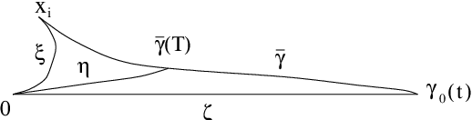
Proof. To prove the first inequality, let η∈Σ⁡(0,γ¯​(T),T+τ)\eta\in\Sigma(0,\overline{\gamma}(T);T+\tau) and let ζ∈Σ⁡(0,γ0​(t),t−τ)\zeta\in\Sigma(0,\gamma_{0}(t);t-\tau). The path ζ\zeta is nothing but a repametrization of γ0|[0,t]\gamma_{0}\left|{}_{[0,t]}\right.. Since η\eta and γ¯\overline{\gamma} are minimizers, we have the triangular inequalities

AL​(η)≤AL(ξ)+AL(γ¯|[0,T])AL​(γ¯)≤AL​(ξ)+AL​(ζ),\begin{array}[]{rl}A_{L}(\eta)&\leq A_{L}(\xi)+A_{L}(\overline{\gamma}\left|{}_{[0,T]}\right.)\\ A_{L}(\overline{\gamma})&\leq A_{L}(\xi)+A_{L}(\zeta),\end{array}

therefore

AL(η)+AL(γ¯|)[T,t]≤AL(ξ)+AL(γ¯)≤2AL(ξ)+AL(ζ).A_{L}(\eta)+A_{L}(\overline{\gamma}\left|{}_{[T,t]}\right.)\leq A_{L}(\xi)+A_{L}(\overline{\gamma})\leq 2A_{L}(\xi)+A_{L}(\zeta).

This gives the first inequality.
The second inequality is a direct consequence of the first one and of Lemma 7.

Refer to caption
Figure 1. The paths γ¯\overline{\gamma}, η\eta, ζ\zeta and ξ\xi in the configuration space.
Proposition 9.

There exist three constants K>0K>0, T¯>0\overline{T}>0 and s¯>1\overline{s}>1 such that for every T≥T¯T\geq\overline{T}, for every t≥s¯​Tt\geq\overline{s}T and for every γ¯∈Σ⁡(xi,γ0​(t),t)\overline{\gamma}\in\Sigma(x_{i},\gamma_{0}(t);t) we have

‖γ¯​(T)‖≤K​T23.\|\overline{\gamma}(T)\|\leq KT^{\frac{2}{3}}.

Proof. Suppose, for the sake of a contradiction, that there exist three sequences of positive real numbers (Kn)n=0+∞(K_{n})_{n=0}^{+\infty}, (Tn)n=0+∞(T_{n})_{n=0}^{+\infty} and (tn)n=0+∞(t_{n})_{n=0}^{+\infty} satisfying

Kn→+∞,Tn→+∞,tnTn→+∞,K_{n}\rightarrow+\infty,\qquad T_{n}\rightarrow+\infty,\qquad\frac{t_{n}}{T_{n}}\rightarrow+\infty,

and a sequence of minimizers γ¯n∈Σ⁡(xi,γ0​(tn),tn)\overline{\gamma}_{n}\in\Sigma(x_{i},\gamma_{0}(t_{n});t_{n}) such that for every n∈ℕn\in{\mathbb{N}} :

‖γ¯n​(Tn)‖≥Kn​Tn23.\|\overline{\gamma}_{n}(T_{n})\|\geq K_{n}T_{n}^{\frac{2}{3}}.

Let τ>0\tau>0 and ξ:[0,τ]→𝒳\xi:[0,\tau]\rightarrow{\mathcal{X}} be a minimizer connecting 00 to xix_{i} in time τ\tau. Without loss of generality we can assume 0<τ<Tn<tn0<\tau<T_{n}<t_{n}. By homothety invariance and by the second inequality of Lemma 8 we have

(10) Tn13​𝒩​(‖γ¯n​(Tn)‖Tn23,α​(tnTn)23,τTn,1,tnTn)≤2​AL​(ξ).T_{n}^{\frac{1}{3}}{\mathcal{N}}\left(\frac{\|\overline{\gamma}_{n}(T_{n})\|}{T_{n}^{\frac{2}{3}}},\alpha\left(\frac{t_{n}}{T_{n}}\right)^{\frac{2}{3}};\frac{\tau}{T_{n}},1,\frac{t_{n}}{T_{n}}\right)\leq 2A_{L}(\xi).

Since ‖γ¯n​(Tn)‖Tn23→+∞\frac{\|\overline{\gamma}_{n}(T_{n})\|}{T_{n}^{\frac{2}{3}}}\rightarrow+\infty and tnTn→+∞\frac{t_{n}}{T_{n}}\rightarrow+\infty, by Proposition 21 of the Appendix we have

𝒩⁡(‖γ¯n​(Tn)‖Tn23,α​(tnTn)23,τTn,1,tnTn)→+∞{\mathcal{N}}\left(\frac{\|\overline{\gamma}_{n}(T_{n})\|}{T_{n}^{\frac{2}{3}}},\alpha\left(\frac{t_{n}}{T_{n}}\right)^{\frac{2}{3}};\frac{\tau}{T_{n}},1,\frac{t_{n}}{T_{n}}\right)\rightarrow+\infty

as n→+∞n\rightarrow+\infty. This contradicts inequality (10).

We need now an estimates of the minimal action 𝒜⁡(x,x′,T){\mathcal{A}}(x,x^{\prime};T) when ‖x‖\|x\| and ‖x′‖\|x^{\prime}\| are less then a given size.

Proposition 10.

There exist two positive constants C1C_{1} and C2C_{2} such that if R>0R>0 and T>0T>0, if x∈𝒳x\in{\mathcal{X}} and x′∈𝒳x^{\prime}\in{\mathcal{X}} are two configurations satisfying ‖x‖≤R\|x\|\leq R and ‖x′‖≤R\|x^{\prime}\|\leq R, we can find an absolutely continuous path γx​x′:[0,T]→𝒳\gamma_{xx^{\prime}}:[0,T]\rightarrow{\mathcal{X}} joining xx to x′x^{\prime} in time TT such that the following inequality holds

(11) AL​(γx​x′)≤C1​R2T+C2​TR.A_{L}(\gamma_{xx^{\prime}})\leq C_{1}\frac{R^{2}}{T}+C_{2}\frac{T}{R}.

In particular we have

(12) 𝒜⁡(x,x′,T)≤C1​R2T+C2​TR.{\mathcal{A}}(x,x^{\prime};T)\leq C_{1}\frac{R^{2}}{T}+C_{2}\frac{T}{R}.

Proof. Let x0′∈𝒳^x_{0}^{\prime}\in{\widehat{\mathcal{X}}} be any normalized collision-free configuration. We construct an absolutely continuous path γx:[0,T/2]→𝒳\gamma_{x}:[0,T/2]\rightarrow{\mathcal{X}} joining xx to R​x0′Rx_{0}^{\prime} and verifying

(13) AL​(γx)≤A1​R2T+A2​TRA_{L}(\gamma_{x})\leq A_{1}\frac{R^{2}}{T}+A_{2}\frac{T}{R}

where A1A_{1} and A2A_{2} are two positive constants independent on RR, TT and xx. An analogous path γx′:[0,T/2]→𝒳\gamma_{x^{\prime}}:[0,T/2]\rightarrow{\mathcal{X}} joining R​x0′Rx_{0}^{\prime} to x′x^{\prime} can be constructed in exactly the same way. Pasting γx\gamma_{x} and γx′\gamma_{x^{\prime}} together and choosing C1=2​A1C_{1}=2A_{1} and C2=2​A2C_{2}=2A_{2} we get a path γx​x′\gamma_{xx^{\prime}} verifying (11). Inequality (12) is an obvious consequence of (11).
Let x0′=(c→1,…,c→N)x_{0}^{\prime}=(\vec{c}_{1},...,\vec{c}_{N}). We term c→i​j=c→j−c→i\vec{c}_{ij}=\vec{c}_{j}-\vec{c}_{i} and ci​j=|c→i​j|c_{ij}=|\vec{c}_{ij}| for 1≤i<j≤N1\leq i<j\leq N. In a similar way, given x=(r→1,…,r→N)∈𝒳x=(\vec{r}_{1},...,\vec{r}_{N})\in{\mathcal{X}} with ‖x‖≤R\|x\|\leq R, we term r→i​j=r→j−r→i\vec{r}_{ij}=\vec{r}_{j}-\vec{r}_{i} and ri​j=|r→i​j|r_{ij}=|\vec{r}_{ij}|. Let λi​j\lambda_{ij} be the coefficients

λi​j=ri​jR​ci​j+ri​j∈[0,1),\lambda_{ij}=\frac{r_{ij}}{Rc_{ij}+r_{ij}}\in[0,1),

and let hh be the cardinality of the set {λi​j}1≤i<j≤N\{\lambda_{ij}\}_{1\leq i<j\leq N}. The inequality 1≤h≤N⁡(N−1)/21\leq h\leq N(N-1)/2 holds. Let us denote

0≤μ1<…<μh<10\leq\mu_{1}<...<\mu_{h}<1

the elements of the set {λi​j}1≤i<j≤N\{\lambda_{ij}\}_{1\leq i<j\leq N} ordered increasingly. We define μ0=0\mu_{0}=0 and μh+1=1\mu_{h+1}=1. For every i=0,…,hi=0,...,h we term

τi=T​(μi+1−μi)322​∑k=0h(μk+1−μk)32.\tau_{i}=\frac{T(\mu_{i+1}-\mu_{i})^{\frac{3}{2}}}{2\sum\limits_{k=0}^{h}(\mu_{k+1}-\mu_{k})^{\frac{3}{2}}}.

We observe that τ0≥0\tau_{0}\geq 0 and τi>0\tau_{i}>0 if i≥1i\geq 1, moreover ∑i=0hτi=T/2\sum\limits_{i=0}^{h}\tau_{i}=T/2. Defining

σ0=0,σi=τ0+…+τi−1,i=1,…,h+1.\sigma_{0}=0,\qquad\sigma_{i}=\tau_{0}+...+\tau_{i-1},\qquad i=1,...,h+1.

we have σh+1=T/2\sigma_{h+1}=T/2. Let λ:[0,T/2]→[0,1]\lambda:[0,T/2]\rightarrow[0,1] be the path defined by

λ⁡(t)={μ1​(1−(τ0−tτ0)23),ift∈[0,σ1]μi+(t−σiτi/2)23​μi+1−μi2,ift∈[σi,σi+τi2],i=1,…,h−1μi+1−(σi+1−tτi/2)23​μi+1−μi2,ift∈[σi+τi2,σi+1],i=1,…,h−1μh+(1−μh)​(t−σhT/2−σh)23,ift∈[σh,T/2].\lambda(t)=\left\{\begin{array}[]{lll}\mu_{1}\left(1-\left(\frac{\tau_{0}-t}{\tau_{0}}\right)^{\frac{2}{3}}\right),&\text{if}\quad t\in[0,\sigma_{1}]&\\ \mu_{i}+\left(\frac{t-\sigma_{i}}{\tau_{i}/2}\right)^{\frac{2}{3}}\frac{\mu_{i+1}-\mu_{i}}{2},&\text{if}\quad t\in[\sigma_{i},\sigma_{i}+\frac{\tau_{i}}{2}],&i=1,...,h-1\\ \mu_{i+1}-\left(\frac{\sigma_{i+1}-t}{\tau_{i}/2}\right)^{\frac{2}{3}}\frac{\mu_{i+1}-\mu_{i}}{2},&\text{if}\quad t\in[\sigma_{i}+\frac{\tau_{i}}{2},\sigma_{i+1}],&i=1,...,h-1\\ \mu_{h}+(1-\mu_{h})\left(\frac{t-\sigma_{h}}{T/2-\sigma_{h}}\right)^{\frac{2}{3}},&\text{if}\quad t\in[\sigma_{h},T/2].&\end{array}\right.

The definition of λ⁡(t)\lambda(t) in the interval [σ0,σ1][\sigma_{0},\sigma_{1}] has some meaning only if σ0<σ1\sigma_{0}<\sigma_{1} (i.e. if τ0>0\tau_{0}>0). The path

γx​(t)=(1−λ⁡(t))​x+λ⁡(t)​R​x0′,t∈[0,T/2]\gamma_{x}(t)=(1-\lambda(t))x+\lambda(t)Rx_{0}^{\prime},\qquad t\in[0,T/2]

connects xx to R​x0′Rx_{0}^{\prime} in the time T/2T/2. If 1≤i≤h−11\leq i\leq h-1, the action of the restriction γx|[σi,σi+τi/2]\gamma_{x}\left|{}_{[\sigma_{i},\sigma_{i}+\tau_{i}/2]}\right. is given by

AL(γx|[σi,σi+τi2])=‖R​x0′−x‖22​∫σiσi+τi2λ˙​(t)2​𝑑t+∑1≤j<k≤Nmjmk∫σiσi+τi2d​t|(1−λ⁡(t))​r→j​k+λ⁡(t)​R​c→j​k|.\begin{array}[]{rl}A_{L}(\gamma_{x}\left|{}_{[\sigma_{i},\sigma_{i}+\frac{\tau_{i}}{2}]}\right.)&=\frac{\|Rx_{0}^{\prime}-x\|^{2}}{2}\displaystyle\int_{\sigma_{i}}^{\sigma_{i}+\frac{\tau_{i}}{2}}\dot{\lambda}(t)^{2}\,dt\\ &+\sum\limits_{1\leq j<k\leq N}m_{j}m_{k}\displaystyle\int_{\sigma_{i}}^{\sigma_{i}+\frac{\tau_{i}}{2}}\frac{dt}{|(1-\lambda(t))\vec{r}_{jk}+\lambda(t)R\vec{c}_{jk}|}.\end{array}

As t∈[σi,σi+τi/2]t\in[\sigma_{i},\sigma_{i}+\tau_{i}/2] the path λ⁡(t)\lambda(t) increases from μi\mu_{i} to (μi+μi+1)/2(\mu_{i}+\mu_{i+1})/2, hence the coefficient λj​k\lambda_{jk} that is closest to λ⁡(t)\lambda(t) is exactly μi\mu_{i}. Using the triangular inequality we find

|(1−λ⁡(t))​r→j​k+λ⁡(t)​R​c→j​k|≥|rj​k−λ⁡(t)​(rj​k+R​cj​k)|=(rj​k+R​cj​k)​|λj​k−λ⁡(t)|≥R​cj​k​|λj​k−λ⁡(t)|≥R​cj​k​(λ⁡(t)−μi),\begin{array}[]{rl}|(1-\lambda(t))\vec{r}_{jk}+\lambda(t)R\vec{c}_{jk}|&\geq|r_{jk}-\lambda(t)(r_{jk}+Rc_{jk})|\\ &=(r_{jk}+Rc_{jk})|\lambda_{jk}-\lambda(t)|\\ &\geq Rc_{jk}|\lambda_{jk}-\lambda(t)|\\ &\geq Rc_{jk}(\lambda(t)-\mu_{i}),\end{array}

for t∈[σi,σi+τi/2]t\in[\sigma_{i},\sigma_{i}+\tau_{i}/2] and for every 1≤j<k≤N1\leq j<k\leq N. Therefore, since ‖x‖≤R\|x\|\leq R and ‖x0′‖=1\|x_{0}^{\prime}\|=1

AL(γx|[σi,σi+τi2])≤2​R2​(μi+1−μi2)2​(2τi)43​∫σiσi+τi249​(t−σi)−23​𝑑t+∑1≤j<k≤Nmj​mkR​cj​k∫σiσi+τi2d​tλ⁡(t)−μi=4​R23​(μi+1−μi)2τi+U⁡(x0′)R​2μi+1−μi​(τi2)23​∫σiσi+τi2d​t(t−σi)23=4​R23​(μi+1−μi)2τi+3​U​(x0′)R​τiμi+1−μi.\begin{array}[]{rl}A_{L}(\gamma_{x}\left|{}_{[\sigma_{i},\sigma_{i}+\frac{\tau_{i}}{2}]}\right.)&\leq 2R^{2}\left(\frac{\mu_{i+1}-\mu_{i}}{2}\right)^{2}\left(\frac{2}{\tau_{i}}\right)^{\frac{4}{3}}\displaystyle\int_{\sigma_{i}}^{\sigma_{i}+\frac{\tau_{i}}{2}}\frac{4}{9}(t-\sigma_{i})^{-\frac{2}{3}}dt\\ &+\sum\limits_{1\leq j<k\leq N}\frac{m_{j}m_{k}}{Rc_{jk}}\displaystyle\int_{\sigma_{i}}^{\sigma_{i}+\frac{\tau_{i}}{2}}\frac{dt}{\lambda(t)-\mu_{i}}\\ &=\frac{4R^{2}}{3}\frac{(\mu_{i+1}-\mu_{i})^{2}}{\tau_{i}}+\frac{U(x_{0}^{\prime})}{R}\frac{2}{\mu_{i+1}-\mu_{i}}\left(\frac{\tau_{i}}{2}\right)^{\frac{2}{3}}\displaystyle\int_{\sigma_{i}}^{\sigma_{i}+\frac{\tau_{i}}{2}}\frac{dt}{(t-\sigma_{i})^{\frac{2}{3}}}\\ &=\frac{4R^{2}}{3}\frac{(\mu_{i+1}-\mu_{i})^{2}}{\tau_{i}}+\frac{3U(x_{0}^{\prime})}{R}\frac{\tau_{i}}{\mu_{i+1}-\mu_{i}}.\end{array}

In a similar way we find

AL(γx|[σi+τi2,σi+1])≤4​R23(μi+1−μi)2τi+3​U​(x0′)Rτiμi+1−μi,i=1,…,h−1AL(γx|[σ0,σ1])≤8​R23​μ12τ0+3​U​(x0′)R​τ0μ1,AL(γx|[σh,σh+1])≤8​R23​(1−μh)2τh+3​U​(x0′)R​τh1−μh.\begin{array}[]{rl}A_{L}(\gamma_{x}\left|{}_{[\sigma_{i}+\frac{\tau_{i}}{2},\sigma_{i+1}]}\right.)&\leq\frac{4R^{2}}{3}\frac{(\mu_{i+1}-\mu_{i})^{2}}{\tau_{i}}+\frac{3U(x_{0}^{\prime})}{R}\frac{\tau_{i}}{\mu_{i+1}-\mu_{i}},\qquad i=1,...,h-1\\ A_{L}(\gamma_{x}\left|{}_{[\sigma_{0},\sigma_{1}]}\right.)&\leq\frac{8R^{2}}{3}\frac{\mu_{1}^{2}}{\tau_{0}}+\frac{3U(x_{0}^{\prime})}{R}\frac{\tau_{0}}{\mu_{1}},\\ A_{L}(\gamma_{x}\left|{}_{[\sigma_{h},\sigma_{h+1}]}\right.)&\leq\frac{8R^{2}}{3}\frac{(1-\mu_{h})^{2}}{\tau_{h}}+\frac{3U(x_{0}^{\prime})}{R}\frac{\tau_{h}}{1-\mu_{h}}.\end{array}

That gives

AL(γx|)[σi,σi+1]≤8​R23(μi+1−μi)2τi+6​U​(x0′)Rτiμi+1−μi,i=0,…,h,A_{L}(\gamma_{x}\left|{}_{[\sigma_{i},\sigma_{i+1}]}\right.)\leq\frac{8R^{2}}{3}\frac{(\mu_{i+1}-\mu_{i})^{2}}{\tau_{i}}+\frac{6U(x_{0}^{\prime})}{R}\frac{\tau_{i}}{\mu_{i+1}-\mu_{i}},\qquad i=0,...,h,

and by definition of τi\tau_{i}

(14) AL​(γx)≤16​R23​T​(∑i=0h(μi+1−μi)32)​(∑i=0h(μi+1−μi)12)+3​U​(x0′)​TR​∑i=0h(μi+1−μi)12∑i=0h(μi+1−μi)32.\begin{array}[]{rl}A_{L}(\gamma_{x})&\leq\frac{16R^{2}}{3T}\left(\sum\limits_{i=0}^{h}(\mu_{i+1}-\mu_{i})^{\frac{3}{2}}\right)\left(\sum\limits_{i=0}^{h}(\mu_{i+1}-\mu_{i})^{\frac{1}{2}}\right)\\ &+\frac{3U(x_{0}^{\prime})T}{R}\frac{\sum\limits_{i=0}^{h}(\mu_{i+1}-\mu_{i})^{\frac{1}{2}}}{\sum\limits_{i=0}^{h}(\mu_{i+1}-\mu_{i})^{\frac{3}{2}}}.\end{array}

By definition of μi\mu_{i} we have

μi+1−μi≥0,∑i=0h(μi+1−μi)=1.\mu_{i+1}-\mu_{i}\geq 0,\qquad\sum\limits_{i=0}^{h}(\mu_{i+1}-\mu_{i})=1.

Let us introduce now the functions

f1:ℝ+h+1→ℝ,f1​(z)=∑i=0hzi32,f2:ℝ+h+1→ℝ,f2​(z)=∑i=0hzi12,g:ℝ+h+1→ℝ,g⁡(z)=∑i=0hzi,\begin{array}[]{rl}f_{1}:{\mathbb{R}}_{+}^{h+1}\rightarrow{\mathbb{R}},\qquad f_{1}(z)&=\sum\limits_{i=0}^{h}z_{i}^{\frac{3}{2}},\\ f_{2}:{\mathbb{R}}_{+}^{h+1}\rightarrow{\mathbb{R}},\qquad f_{2}(z)&=\sum\limits_{i=0}^{h}z_{i}^{\frac{1}{2}},\\ g:{\mathbb{R}}_{+}^{h+1}\rightarrow{\mathbb{R}},\qquad g(z)&=\sum\limits_{i=0}^{h}z_{i},\end{array}

and study minima and maxima of f1f_{1} and f2f_{2} under the condition g⁡(z)=1g(z)=1. We show by induction on hh that

(15) ming⁡(z)=1⁡f1​(z)=1(h+1)12,maxg⁡(z)=1⁡f1​(z)=1.\min\limits_{g(z)=1}f_{1}(z)=\frac{1}{(h+1)^{\frac{1}{2}}},\qquad\max\limits_{g(z)=1}f_{1}(z)=1.

If h=0h=0, condition g⁡(z)=1g(z)=1 implies z0=1z_{0}=1, thus

ming⁡(z)=1⁡f1​(z)=1,maxg⁡(z)=1⁡f1​(z)=1\min\limits_{g(z)=1}f_{1}(z)=1,\qquad\max\limits_{g(z)=1}f_{1}(z)=1

Assuming now the statement is true up to order h−1h-1, let us prove it is true at order hh. By Lagrange multiplier theorem, the unique interior critical point of f1f_{1} under the condition g⁡(z)=1g(z)=1 is given by the equations

∂f1∂zi(z)=λ∂g∂zi(z),i=0,…,h,λ∈ℝ,g(z)=1,\frac{\partial f_{1}}{\partial z_{i}}(z)=\lambda\frac{\partial g}{\partial z_{i}}(z),\quad i=0,...,h,\qquad\lambda\in{\mathbb{R}},\qquad g(z)=1,

this gives

zi=1h+1,i=0,…,h,f1(z)=1(h+1)12.z_{i}=\frac{1}{h+1},\quad i=0,...,h,\qquad f_{1}(z)=\frac{1}{(h+1)^{\frac{1}{2}}}.

The boundary of the simplex g⁡(z)=1g(z)=1 is the set of z=(z0,…,zh)z=(z_{0},...,z_{h}) such that ∑i=0hzi=1\sum\limits_{i=0}^{h}z_{i}=1 and zi=0z_{i}=0 for at least one indices ii. By inductive hypothesis, the minimum of f1​(z)f_{1}(z) on the boundary of g⁡(z)=1g(z)=1 is 1/h1/21/h^{1/2} and the maximum is 11. Comparing with the value of f1f_{1} on the unique interior critical point of f1f_{1} we find (15). In a similar way one prove

(16) ming⁡(z)=1⁡f2​(z)=1,maxg⁡(z)=1⁡f2​(z)=(h+1)12.\min\limits_{g(z)=1}f_{2}(z)=1,\qquad\max\limits_{g(z)=1}f_{2}(z)=(h+1)^{\frac{1}{2}}.

Replacing these estimates in (14) we find

AL​(γx)≤16​R23​T​(h+1)12+3​U​(x0′)​TR​(h+1),A_{L}(\gamma_{x})\leq\frac{16R^{2}}{3T}(h+1)^{\frac{1}{2}}+\frac{3U(x_{0}^{\prime})T}{R}(h+1),

since h≤N⁡(N−1)2h\leq\frac{N(N-1)}{2}, inequality (13) is proved.

We give now the proof of Theorem 6.
Proof of Theorem 6. By Propositions 9 and 10, there exist three constants a>0a>0, T¯>0\overline{T}>0 and s¯>1\overline{s}>1 such that for every T≥T¯T\geq\overline{T}, for every t≥s¯​Tt\geq\overline{s}T and for every minimizer γ¯∈Σ⁡(xi,γ0​(t),t)\overline{\gamma}\in\Sigma(x_{i},\gamma_{0}(t);t) we have

(17) AL(γ¯|)[0,T]≤aT13A_{L}(\overline{\gamma}\left|{}_{[0,T]}\right.)\leq aT^{\frac{1}{3}}

Let us prove the equicontinuity of the family

(18) {γ¯|,[0,T]γ¯∈Σ(xi,γ0(t);t),t≥s¯T}.\left\{\overline{\gamma}\left|{}_{[0,T]}\right.,\quad\overline{\gamma}\in\Sigma(x_{i},\gamma_{0}(t);t),\quad t\geq\overline{s}T\right\}.

By (17) we have

∫0T‖γ¯˙​(s)‖2​𝑑s≤2​a​T13,\int_{0}^{T}\|\dot{\overline{\gamma}}(s)\|^{2}ds\leq 2aT^{\frac{1}{3}},

hence, by Cauchy-Schwarz inequality, for every 0≤s<s′≤T0\leq s<s^{\prime}\leq T we have

|γ¯​(s′)−γ¯​(s)|≤∫ss′‖γ¯˙​(u)‖​𝑑u≤s−s′​(∫ss′‖γ¯˙​(u)‖2​𝑑u)12≤(2​a​T13)12​s−s′.\begin{array}[]{rl}|\overline{\gamma}(s^{\prime})-\overline{\gamma}(s)|\leq\displaystyle\int_{s}^{s^{\prime}}\|\dot{\overline{\gamma}}(u)\|du&\leq\sqrt{s-s^{\prime}}\left(\displaystyle\int_{s}^{s^{\prime}}\|\dot{\overline{\gamma}}(u)\|^{2}du\right)^{\frac{1}{2}}\\ &\leq(2aT^{\frac{1}{3}})^{\frac{1}{2}}\sqrt{s-s^{\prime}}.\end{array}

This gives the equicontinuity of the family (18). By the way, since γ¯​(0)=xi\overline{\gamma}(0)=x_{i}, the family is also equibounded. By Ascoli theorem we can find a divergent sequence (tn)n=1+∞(t_{n})_{n=1}^{+\infty} satisfying tn≥s¯​Tt_{n}\geq\overline{s}T and and a sequence of minimizers γn∈Σ⁡(xi,γ0​(tn),tn)\gamma_{n}\in\Sigma(x_{i},\gamma_{0}(t_{n});t_{n}) such that the restriction (γn|)[0,T]n=1+∞(\gamma_{n}\left|{}_{[0,T]}\right.)_{n=1}^{+\infty} converges uniformly. Applying this argument on an increasing and divergent sequence (Tk)k=1+∞(T_{k})_{k=1}^{+\infty}, by a diagonal trick we can find an increasing and divergent sequence of times (tn)n=1+∞(t_{n})_{n=1}^{+\infty}, a sequence of minimizers γn∈Σ⁡(xi,γ0​(tn),tn)\gamma_{n}\in\Sigma(x_{i},\gamma_{0}(t_{n});t_{n}) and a path γ:[0,+∞)→𝒳\gamma:[0,+\infty)\rightarrow{\mathcal{X}} such that (γn)n=1+∞(\gamma_{n})_{n=1}^{+\infty} converges uniformly to γ\gamma on every compact interval. Moreover, by lower semi-continuity of the action we have

(19) AL(γ|)[0,T]≤lim infn→+∞AL(γn|)[0,T]≤aT13A_{L}(\gamma\left|{}_{[0,T]}\right.)\leq\liminf\limits_{n\rightarrow+\infty}A_{L}(\gamma_{n}\left|{}_{[0,T]}\right.)\leq aT^{\frac{1}{3}}

for every T>0T>0, proving in particular that AL(γ|)[0,T]A_{L}(\gamma\left|{}_{[0,T]}\right.) is finite. Therefore, γ⁡(T)\gamma(T) is a non-collision configuration for almost all T>0T>0. We prove now that γ\gamma is a minimizing path. Since we want to show that γ|[0,T]\gamma\left|{}_{[0,T]}\right. is a minimizer for every T>0T>0, it is sufficient to prove that γ|[0,T]\gamma\left|{}_{[0,T]}\right. is a minimizer for TT arbitrary great.

Refer to caption
Figure 2. σϵ,n\sigma_{\epsilon,n} is obtained by pasting σ\sigma (reparametrized) with the straight line joining γ⁡(T)\gamma(T) to γn​(T)\gamma_{n}(T)

We can assume, without loss of generality, that γ⁡(T)\gamma(T) is a non-collision configuration. Assuming, for the sake of a contradiction, that γ|[0,T]\gamma\left|{}_{[0,T]}\right. is not a minimizer, there would exists an absolutely continuous path σ:[0,T]→𝒳\sigma:[0,T]\rightarrow{\mathcal{X}} joining xix_{i} to γ⁡(T)\gamma(T) such that

(20) AL(σ)<AL(γ|)[0,T].A_{L}(\sigma)<A_{L}(\gamma\left|{}_{[0,T]}\right.).

Moreover, there exists M>0M>0 and ϵ¯>0\overline{\epsilon}>0 such that

∀x∈B¯​(γ⁡(T),ϵ¯)⇒U⁡(x)≤M,\forall x\in\overline{B}(\gamma(T),\overline{\epsilon})\Rightarrow U(x)\leq M,

where B¯​(γ​(T),ϵ¯)\overline{B}(\gamma(T),\overline{\epsilon}) is the closed ball centered in γ⁡(T)\gamma(T) with radius ϵ¯\overline{\epsilon}. Since the sequence γn|[0,T]\gamma_{n}\left|{}_{[0,T]}\right. converges uniformly to γ|[0,T]\gamma\left|{}_{[0,T]}\right., given 0<ϵ<ϵ¯0<\epsilon<\overline{\epsilon} there exists a positive integer NT,ϵN_{T,\epsilon} such that for every n≥NT,ϵn\geq N_{T,\epsilon} we have γn​(T)∈B¯​(γ⁡(T),ϵ)\gamma_{n}(T)\in\overline{B}(\gamma(T),\epsilon). Let σϵ,n:[0,T]→𝒳\sigma_{\epsilon,n}:[0,T]\rightarrow{\mathcal{X}} be the path defined by

σϵ,n​(t)={σ⁡(TT−ϵ​t)ift∈[0,T−ϵ]T−tϵ​γ​(T)+t−T+ϵϵ​γn​(T)ift∈[T−ϵ,T],\sigma_{\epsilon,n}(t)=\left\{\begin{array}[]{ll}\sigma(\frac{T}{T-\epsilon}t)&\text{if}\quad t\in[0,T-\epsilon]\\ \frac{T-t}{\epsilon}\gamma(T)+\frac{t-T+\epsilon}{\epsilon}\gamma_{n}(T)&\text{if}\quad t\in[T-\epsilon,T],\end{array}\right.

where n≥NT,ϵn\geq N_{T,\epsilon}. By construction σϵ,n\sigma_{\epsilon,n} joins xix_{i} to γn​(T)\gamma_{n}(T) in time TT (see Figure 2). Moreover, if t∈[T−ϵ,T]t\in[T-\epsilon,T], σϵ,n​(t)\sigma_{\epsilon,n}(t) is contained in the ball B¯​(γ​(T),ϵ)\overline{B}(\gamma(T),\epsilon). Computing the action of σϵ,n\sigma_{\epsilon,n} we get

AL​(σϵ,n)≤12​(TT−ϵ)2​∫0T−ϵ‖σ˙​(T​tT−ϵ)‖2​𝑑t+∫0T−ϵU⁡(σ⁡(T​tT−ϵ))​𝑑t+(M+12)​ϵ=TT−ϵ​∫0T12​‖σ˙​(t)‖2​𝑑t+T−ϵT​∫0TU⁡(σ⁡(t))​𝑑t+(M+12)​ϵ=AL​(σ)+𝒪⁡(ϵ).\begin{array}[]{rl}A_{L}(\sigma_{\epsilon,n})&\leq\frac{1}{2}\left(\frac{T}{T-\epsilon}\right)^{2}\displaystyle\int_{0}^{T-\epsilon}\left\|\dot{\sigma}\left(\frac{Tt}{T-\epsilon}\right)\right\|^{2}dt+\displaystyle\int_{0}^{T-\epsilon}U\left(\sigma\left(\frac{Tt}{T-\epsilon}\right)\right)dt\\ &+\left(M+\frac{1}{2}\right)\epsilon\\ &=\frac{T}{T-\epsilon}\displaystyle\int_{0}^{T}\frac{1}{2}\|\dot{\sigma}(t)\|^{2}dt+\frac{T-\epsilon}{T}\displaystyle\int_{0}^{T}U(\sigma(t))dt+\left(M+\frac{1}{2}\right)\epsilon\\ &=A_{L}(\sigma)+{\mathcal{O}}(\epsilon).\end{array}

Inequalities (19) and (20) imply

AL(σϵ,n)<AL(γn|)[0,T]A_{L}(\sigma_{\epsilon,n})<A_{L}(\gamma_{n}\left|{}_{[0,T]}\right.)

if ϵ\epsilon is sufficiently small and nn sufficiently great. This contradicts the minimizing property of γn\gamma_{n} and proves that γ\gamma is a minimizer. By Marchal theorem, γ\gamma is collision-free (and in particular it is a real solution of the N-body problem) for t>0t>0. This complete the proof of Theorem 6.

4. Parabolicity of the solution

To complete the proof of the main theorem we still have to show that the limit solution γ⁡(t)\gamma(t) is parabolic and asymptotic to x0x_{0}. By Lemma 5 we just need to verify the asymptotic estimates (6). We introduce now the following

Notation.

Given the functions f⁡(r,x1,…,xn)f(r,x_{1},...,x_{n}) and g⁡(r,x1,…,xn)≠0g(r,x_{1},...,x_{n})\neq 0, we write f⁡(r,x1,…,xn)=or​(g⁡(r,x1,…,xn))f(r,x_{1},...,x_{n})=o_{r}(g(r,x_{1},...,x_{n})) as r→r0r\rightarrow r_{0} if the quotient f⁡(r,x1,…,xn)g⁡(r,x1,…,xn)\frac{f(r,x_{1},...,x_{n})}{g(r,x_{1},...,x_{n})} is infinitesimal as r→r0r\rightarrow r_{0}, uniformly on (x1,…,xn)(x_{1},...,x_{n}). In a similar way, we write f⁡(r,x1,…,xn)=𝒪r​(g⁡(r,x1,…,xn))f(r,x_{1},...,x_{n})={\mathcal{O}}_{r}(g(r,x_{1},...,x_{n})) if the quotient f⁡(r,x1,…,xn)g⁡(r,x1,…,xn)\frac{f(r,x_{1},...,x_{n})}{g(r,x_{1},...,x_{n})} is locally bounded for rr close to r0r_{0}, uniformly on the variables (x1,…,xn)(x_{1},...,x_{n}).

Let us give now a refinement of Lemma 8.

Lemma 11.

Let τ>0\tau>0 and ξ∈Σ⁡(0,xi,τ)\xi\in\Sigma(0,x_{i};\tau). There exist two constants T¯>τ\overline{T}>\tau and s¯>1\overline{s}>1 such that for every T≥T¯T\geq\overline{T}, for every t≥s¯​Tt\geq\overline{s}T and for every minimizer γ¯∈Σ⁡(xi,γ0​(t),t)\overline{\gamma}\in\Sigma(x_{i},\gamma_{0}(t);t) we have

ℳ⁡(γ¯​(T),γ0​(t),0,T,t)≤2​AL​(ξ)+𝒪T​(T−23)𝒩⁡(‖γ¯​(T)‖,α​t23,0,T,t)≤2​AL​(ξ)+𝒪T​(T−23).\begin{array}[]{rl}{\mathcal{M}}(\overline{\gamma}(T),\gamma_{0}(t);0,T,t)&\leq 2A_{L}(\xi)+{\mathcal{O}}_{T}(T^{-\frac{2}{3}})\\ {\mathcal{N}}(\|\overline{\gamma}(T)\|,\alpha t^{\frac{2}{3}};0,T,t)&\leq 2A_{L}(\xi)+{\mathcal{O}}_{T}(T^{-\frac{2}{3}}).\end{array}

as T→+∞T\rightarrow+\infty.

Proof. The second inequality is a direct consequence of the first one and of Lemma 7. Let us prove the first inequality. We consider τ\tau as a fixed constant, while TT and tt are variables. Let T¯>0\overline{T}>0, s¯>1\overline{s}>1 and K>0K>0 be like in Proposition 9. Without loss of generality we can assume T¯>τ\overline{T}>\tau. Let T≥T¯T\geq\overline{T} and t≥s¯​Tt\geq\overline{s}T. Let ηT+τ∈Σ⁡(0,γ¯​(T),T+τ)\eta_{T+\tau}\in\Sigma(0,\overline{\gamma}(T);T+\tau) The path

η¯T:[0,T]→𝒳,η¯T​(s)=ηT+τ​(T+τT​s).\overline{\eta}_{T}:[0,T]\rightarrow{\mathcal{X}},\qquad\overline{\eta}_{T}(s)=\eta_{T+\tau}\left(\frac{T+\tau}{T}s\right).

is a reparametrization of ηT+τ\eta_{T+\tau} and it joins 00 to γ¯​(T)\overline{\gamma}(T) in time TT, thus

𝒜⁡(0,γ¯​(T),T)≤AL​(η¯T).{\mathcal{A}}(0,\overline{\gamma}(T);T)\leq A_{L}(\overline{\eta}_{T}).

A computation of the action of η¯T\overline{\eta}_{T} gives

(21) AL​(η¯T)=(1+𝒪⁡(1/T))​AL​(ηT+τ),T→+∞.A_{L}(\overline{\eta}_{T})=\left(1+{\mathcal{O}}(1/T)\right)A_{L}(\eta_{T+\tau}),\qquad T\rightarrow+\infty.

Since ηT+τ\eta_{T+\tau} is a minimizer joining 00 to γ¯​(T)\overline{\gamma}(T) in time T+τT+\tau, by Propositions 9 and 10 we obtain

(22) AL​(ηT+τ)≤C1​K2​T43T+τ+C2​T+τK​T23=𝒪⁡(T13).A_{L}(\eta_{T+\tau})\leq C_{1}\frac{K^{2}T^{\frac{4}{3}}}{T+\tau}+C_{2}\frac{T+\tau}{KT^{\frac{2}{3}}}={\mathcal{O}}(T^{\frac{1}{3}}).

Combining inequalities (21) and (22), by definition of ηT+τ\eta_{T+\tau} and η¯T\overline{\eta}_{T} we get

(23) 𝒜⁡(0,γ¯​(T),T)−𝒜⁡(0,γ¯​(T),T+τ)≤𝒪⁡(T−23).T→+∞{\mathcal{A}}(0,\overline{\gamma}(T);T)-{\mathcal{A}}(0,\overline{\gamma}(T);T+\tau)\leq{\mathcal{O}}(T^{-\frac{2}{3}}).\quad T\rightarrow+\infty

In a similar way, let us consider a minimizer ηT∈Σ⁡(0,γ¯​(T),T)\eta_{T}\in\Sigma(0,\overline{\gamma}(T);T) The path

η¯T+τ:[0,T+τ]→𝒳,η¯T+τ​(s)=ηT​((TT+τ)​s).\overline{\eta}_{T+\tau}:[0,T+\tau]\rightarrow{\mathcal{X}},\qquad\overline{\eta}_{T+\tau}(s)=\eta_{T}\left(\left(\frac{T}{T+\tau}\right)s\right).

is a reparametrization of ηT\eta_{T}, and it joins 00 to γ¯​(T)\overline{\gamma}(T) in time T+τT+\tau, hence

𝒜⁡(0,γ¯​(T),T+τ)≤AL​(η¯T+τ).{\mathcal{A}}(0,\overline{\gamma}(T);T+\tau)\leq A_{L}(\overline{\eta}_{T+\tau}).

Arguing as before we get the estimates

(24) 𝒜⁡(0,γ¯​(T),T+τ)−𝒜⁡(0,γ¯​(T),T)≤𝒪⁡(T−23),T→+∞.{\mathcal{A}}(0,\overline{\gamma}(T);T+\tau)-{\mathcal{A}}(0,\overline{\gamma}(T);T)\leq{\mathcal{O}}(T^{-\frac{2}{3}}),\quad T\rightarrow+\infty.

Combining inequalities (23) with (24) we obtain

(25) 𝒜⁡(0,γ¯​(T),T+τ)=𝒜⁡(0,γ¯​(T),T)+𝒪T​(T−23),T→+∞,{\mathcal{A}}(0,\overline{\gamma}(T);T+\tau)={\mathcal{A}}(0,\overline{\gamma}(T);T)+{\mathcal{O}}_{T}(T^{-\frac{2}{3}}),\quad T\rightarrow+\infty,

uniformly on t≥s¯​Tt\geq\overline{s}T and γ¯∈Σ⁡(0,γ0​(t),t)\overline{\gamma}\in\Sigma(0,\gamma_{0}(t);t). With the same argument we find the following estimates

(26) 𝒜⁡(0,γ0​(t),t−τ)−𝒜⁡(0,γ0​(t),t)=𝒪t​(t−23),t→+∞.{\mathcal{A}}(0,\gamma_{0}(t);t-\tau)-{\mathcal{A}}(0,\gamma_{0}(t);t)={\mathcal{O}}_{t}(t^{-\frac{2}{3}}),\quad t\rightarrow+\infty.

Replacing (25) and (26) into the first inequality of Lemma 8, since we assume t≥s¯​Tt\geq\overline{s}T and s¯>1\overline{s}>1, we obtain the first inequality of this Lemma. This ends the proof.

To simplify the notations we introduce now the functions

ℱ:𝒳×(1,+∞)→ℝ+ℱ⁡(x,s)=ℳ⁡(x,γ0​(s),0,1,s)=𝒜⁡(0,x,1)+𝒜⁡(x,γ0​(s),s−1)−𝒜⁡(0,γ0​(s),s),\begin{array}[]{rl}&{\mathcal{F}}:{\mathcal{X}}\times(1,+\infty)\rightarrow{\mathbb{R}}_{+}\\ &{\mathcal{F}}(x,s)={\mathcal{M}}(x,\gamma_{0}(s);0,1,s)={\mathcal{A}}(0,x;1)+{\mathcal{A}}(x,\gamma_{0}(s);s-1)-{\mathcal{A}}(0,\gamma_{0}(s);s),\end{array}

and

𝒢:ℝ+×(1,+∞)→ℝ+𝒢⁡(r,s)=𝒩⁡(r,α​s23,0,1,s)=S⁡(0,r,1)+S⁡(r,α​s23,s−1)−S⁡(0,α​s23,s).\begin{array}[]{rl}&{\mathcal{G}}:{\mathbb{R}}_{+}\times(1,+\infty)\rightarrow{\mathbb{R}}_{+}\\ &{\mathcal{G}}(r,s)={\mathcal{N}}(r,\alpha s^{\frac{2}{3}};0,1,s)=S(0,r;1)+S(r,\alpha s^{\frac{2}{3}};s-1)-S(0,\alpha s^{\frac{2}{3}};s).\end{array}
Lemma 12.

Given s>1s>1 and x∈𝒳x\in{\mathcal{X}} we have

ℱ⁡(x,s)≥0{\mathcal{F}}(x,s)\geq 0

with equality if and only if x=α​x0x=\alpha x_{0}.

Proof. By Lemma 7 we have

ℱ⁡(x,s)≥𝒢⁡(‖x‖,s),{\mathcal{F}}(x,s)\geq{\mathcal{G}}(\|x\|,s),

with equality if and only if x=‖x‖​x0x=\|x\|x_{0}. Since u↦α​u23u\mapsto\alpha u^{\frac{2}{3}} is the unique solution of the one-dimensional Kepler problem joining 00 to α​s23\alpha s^{\frac{2}{3}} in time ss (see Lemma 16 in the Appendix), it is also a minimizer, therefore

𝒢⁡(r,s)≥0,{\mathcal{G}}(r,s)\geq 0,

with equality if and only if r=αr=\alpha. This proves the Lemma.

By homothety invariance, the conclusion of Lemmas 11 and 12 can be written in the more compact form

(27) 0≤T1/3​ℱ​(γ¯​(T)T2/3,tT)≤2AL(ξ)+𝒪T(T−2/3)0≤T1/3​𝒢​(‖γ¯​(T)‖T2/3,tT)≤2AL(ξ)+𝒪T(T−2/3).\begin{array}[]{rl}0\leq T^{1/3}{\mathcal{F}}\left(\frac{\overline{\gamma}(T)}{T^{2/3}},\frac{t}{T}\right)&\leq 2A_{L}(\xi)+{\mathcal{O}}_{T}(T^{-{2/3}})\\ 0\leq T^{1/3}{\mathcal{G}}\left(\frac{\|\overline{\gamma}(T)\|}{T^{2/3}},\frac{t}{T}\right)&\leq 2A_{L}(\xi)+{\mathcal{O}}_{T}(T^{-{2/3}}).\end{array}

as T→+∞T\rightarrow+\infty, uniformly on t≥s¯​Tt\geq\overline{s}T and γ¯∈Σ⁡(0,γ0​(t),t)\overline{\gamma}\in\Sigma(0,\gamma_{0}(t);t).
The following Theorem is a main tool in the proof of the Main Theorem. It shows that if ℱ⁡(x,s){\mathcal{F}}(x,s) is sufficiently small and ss is sufficiently great, the configuration xx is close to α​x0\alpha x_{0}.

Theorem 13.

There exist a function δ:(0,ϵ¯]→ℝ+\delta:(0,\overline{\epsilon}]\rightarrow{\mathbb{R}}_{+} satisfying δ⁡(ϵ)=o⁡(1)\delta(\epsilon)=o(1) as ϵ→0+\epsilon\rightarrow 0^{+}, such that for every ϵ∈(0,ϵ¯]\epsilon\in(0,\overline{\epsilon}], there exists s¯ϵ>1\overline{s}_{\epsilon}>1, such that for every s≥s¯ϵs\geq\overline{s}_{\epsilon}, the set of configurations x∈𝒳x\in{\mathcal{X}} satisfying the inequality

(28) ℱ⁡(x,s)≤ϵ{\mathcal{F}}(x,s)\leq\epsilon

is contained in the ball B¯​(α​x0,δ⁡(ϵ)){\overline{B}}(\alpha x_{0},\delta(\epsilon)).

Before giving the proof of Theorem 13, we show that this theorem achieve the proof of the Main Theorem.
Proof of the Main Theorem. Let γ:[0,+∞)→𝒳\gamma:[0,+\infty)\rightarrow{\mathcal{X}} be the limit solution constructed in Theorem 6 and let γn∈Σ⁡(xi,γ0​(tn),tn)\gamma_{n}\in\Sigma(x_{i},\gamma_{0}(t_{n});t_{n}) be the sequence of minimizers uniformly convergent to γ\gamma on every compact interval. Let ϵ¯\overline{\epsilon} like in Theorem 13 and 0<ϵ<ϵ¯0<\epsilon<\overline{\epsilon}. An immediate consequence of inequalities (27) is the existence of T¯ϵ≥T¯\overline{T}_{\epsilon}\geq\overline{T} such that if T≥T¯ϵT\geq\overline{T}_{\epsilon} and tn≥s¯​Tt_{n}\geq\overline{s}T we have

ℱ⁡(γn​(T)T23,tnT)≤ϵ{\mathcal{F}}\left(\frac{\gamma_{n}(T)}{T^{\frac{2}{3}}},\frac{t_{n}}{T}\right)\leq\epsilon

and by Theorem 13

‖γn​(T)T2/3−α​x0‖≤δ⁡(ϵ),\left\|\frac{\gamma_{n}(T)}{T^{2/3}}-\alpha x_{0}\right\|\leq\delta(\epsilon),

for tnt_{n} sufficiently great. The sequence γn|[0,T]\gamma_{n}\left|{}_{[0,T]}\right. converges uniformly to γ|[0,T]\gamma\left|{}_{[0,T]}\right. as n→+∞n\rightarrow+\infty, hence

‖γ⁡(T)T2/3−α​x0‖≤δ⁡(ϵ),\left\|\frac{\gamma(T)}{T^{2/3}}-\alpha x_{0}\right\|\leq\delta(\epsilon),

for every T≥T¯ϵT\geq\overline{T}_{\epsilon}. Since δ⁡(ϵ)→0\delta(\epsilon)\rightarrow 0 as ϵ→0\epsilon\rightarrow 0, we have proved that

γ⁡(T)T2/3→α​x0,asT→+∞,\frac{\gamma(T)}{T^{2/3}}\rightarrow\alpha x_{0},\quad\text{as}\quad T\rightarrow+\infty,

that is to say, γ\gamma is parabolic and asymptotic to x0x_{0}. This achieves the proof of the Main Theorem.
The next section is devoted to prove Theorem 13.

5. Proof of Theorem 13

In order to achieve the proof of Theorem 13 we compare the NN-body problem with a Kepler problem on the configuration space with a lagrangian given by

L0​(x,x˙)=‖x˙‖22+U0‖x‖,(x,x˙)∈𝒳×𝒳.L_{0}(x,\dot{x})=\frac{\|\dot{x}\|^{2}}{2}+\frac{U_{0}}{\|x\|},\qquad(x,\dot{x})\in{\mathcal{X}}\times{\mathcal{X}}.

Let AL0​(ϖ)A_{L_{0}}(\varpi) denote the action (for the lagrangian L0L_{0}) of an absolutely continuous path ϖ\varpi and 𝒜0​(x1,x2,s){\mathcal{A}}_{0}(x_{1},x_{2};s) the infimum of AL0​(ϖ)A_{L_{0}}(\varpi) over all absolutely continuous paths ϖ\varpi joining x1x_{1} to x2x_{2} in time ss. We have the inequality

𝒜⁡(x1,x2,s)≥𝒜0​(x1,x2,s)≥S⁡(‖x1‖,‖x2‖,s),{\mathcal{A}}(x_{1},x_{2};s)\geq{\mathcal{A}}_{0}(x_{1},x_{2};s)\geq S(\|x_{1}\|,\|x_{2}\|;s),

with 𝒜⁡(x1,x2,s)=𝒜0​(x1,x2,s){\mathcal{A}}(x_{1},x_{2};s)={\mathcal{A}}_{0}(x_{1},x_{2};s) if and only if there exists a minimizing path (for the lagrangian LL) ϖ:[0,s]→𝒳\varpi:[0,s]\rightarrow{\mathcal{X}} joining x1x_{1} with x2x_{2} such that U~​(ϖ​(u))=U0\tilde{U}(\varpi(u))=U_{0} for every u∈[0,s]u\in[0,s], and 𝒜0​(x1,x2,s)=S⁡(‖x1‖,‖x2‖,s){\mathcal{A}}_{0}(x_{1},x_{2};s)=S(\|x_{1}\|,\|x_{2}\|;s) if and only if x1x_{1} and x2x_{2} are on a same half-line starting from the origin. The function

ℱ0:𝒳×(1,+∞)→ℝ+,ℱ0​(x,s)=𝒜0​(0,x,1)+𝒜0​(x,γ0​(s),s−1)−𝒜0​(0,γ0​(s),s),\begin{array}[]{rl}&{\mathcal{F}}_{0}:{\mathcal{X}}\times(1,+\infty)\rightarrow{\mathbb{R}}_{+},\\ &{\mathcal{F}}_{0}(x,s)={\mathcal{A}}_{0}(0,x;1)+{\mathcal{A}}_{0}(x,\gamma_{0}(s);s-1)-{\mathcal{A}}_{0}(0,\gamma_{0}(s);s),\end{array}

verifies the inequality

(29) ℱ⁡(x,s)≥ℱ0​(x,s)≥𝒢⁡(‖x‖,s)≥0.{\mathcal{F}}(x,s)\geq{\mathcal{F}}_{0}(x,s)\geq{\mathcal{G}}(\|x\|,s)\geq 0.

Roughly speaking, to achieve the proof of Theorem 13, we replace ℱ⁡(x,s){\mathcal{F}}(x,s) with ℱ0​(x,s){\mathcal{F}}_{0}(x,s) and we show that if ϵ\epsilon is small and ss great, the inequality ℱ0​(x,s)≤ϵ{\mathcal{F}}_{0}(x,s)\leq\epsilon can be satisfied only if xx is in a small ball centered in α​x0\alpha x_{0}.
This goal will be achieved in two steps. In Proposition 14 we prove that if ss is sufficiently great, the set of r∈ℝ+r\in{\mathbb{R}}_{+} verifying 𝒢⁡(r,s)≤ϵ{\mathcal{G}}(r,s)\leq\epsilon is contained in a small interval centered in α\alpha. Hence, by inequality (29), the set of configuration xx verifying ℱ⁡(x,s)≤ϵ{\mathcal{F}}(x,s)\leq\epsilon is contained in a thin hollow sphere with inner and outer radious close to α\alpha. In Proposition 15 we show that the set of configurations xx verifying ℱ0​(x,s)≤ϵ{\mathcal{F}}_{0}(x,s)\leq\epsilon is a small neighborhood of α​x0\alpha x_{0}.

Proposition 14.

There exist a function δ1:(0,ϵ¯1]→ℝ+\delta_{1}:(0,\overline{\epsilon}_{1}]\rightarrow{\mathbb{R}}_{+} satisfying δ1​(ϵ)=o​(1)\delta_{1}(\epsilon)=o(1) as ϵ→0+\epsilon\rightarrow 0^{+}, such that for every ϵ∈(0,ϵ¯1]\epsilon\in(0,\overline{\epsilon}_{1}] there exists s¯ϵ1>1\overline{s}^{1}_{\epsilon}>1, such that for every s≥s¯ϵ1s\geq\overline{s}^{1}_{\epsilon}, the set of r∈ℝ+r\in{\mathbb{R}}_{+} satisfying the inequality

𝒢⁡(r,s)≤ϵ{\mathcal{G}}(r,s)\leq\epsilon

is contained in the interval [α−δ1​(ϵ),α+δ1​(ϵ)][\alpha-\delta_{1}(\epsilon),\alpha+\delta_{1}(\epsilon)] .

Proof. By Proposition 21 of the Appendix there exists r¯>0\overline{r}>0 and s¯>0\overline{s}>0 such that for every r≥r¯r\geq\overline{r} and for every s≥s¯s\geq\overline{s} we have 𝒢⁡(r,s)>1{\mathcal{G}}(r,s)>1. Without loss of generality we will assume α<r¯<s¯1/3\alpha<\overline{r}<\overline{s}^{1/3}. By Proposition 20 of the Appendix we have

𝒢⁡(r,s)=S⁡(0,r,1)−β0​r12+g⁡(r,s),{\mathcal{G}}(r,s)=S(0,r;1)-\beta_{0}r^{\frac{1}{2}}+g(r,s),

where g​(r,s)=os​(1)g(r,s)=o_{s}(1) as s→+∞s\rightarrow+\infty, uniformly on 0≤r≤s130\leq r\leq s^{\frac{1}{3}}, and where β0=(8​U0)12\beta_{0}=(8U_{0})^{\frac{1}{2}}. Let us introduce now the function

G⁡(r)=S⁡(0,r,1)−β0​r12.G(r)=S(0,r;1)-\beta_{0}r^{\frac{1}{2}}.

By Lemma 16 the solution joining 00 with rr in time 11 is monotonic if and only if for r≥βr\geq\beta, where β=2​(U0π2)1/3\beta=2\left(\frac{U_{0}}{\pi^{2}}\right)^{1/3}. We remark that β<α\beta<\alpha. The energy h⁡(0,r,1)h(0,r;1) of this solution is negative if and only if 0≤r<α0\leq r<\alpha, moreover h(0,β;1)=−U0/βh(0,\beta;1)=-U_{0}/\beta. Let us term h=h⁡(0,r,1)h=h(0,r;1). The action S⁡(0,r,1)S(0,r;1) is given by

S⁡(0,r,1)={∫0−U0h2​(h+U0u)​𝑑u+∫r−U0h2​(h+U0u)​𝑑u−hifr<β∫0r2​(h+U0u)​𝑑u−hifr≥β,S(0,r;1)=\left\{\begin{array}[]{ll}\displaystyle\int_{0}^{-\frac{U_{0}}{h}}\sqrt{2\left(h+\frac{U_{0}}{u}\right)}du+\displaystyle\int_{r}^{-\frac{U_{0}}{h}}\sqrt{2\left(h+\frac{U_{0}}{u}\right)}du-h&\text{if}\quad r<\beta\\ \displaystyle\int_{0}^{r}\sqrt{2\left(h+\frac{U_{0}}{u}\right)}du-h&\text{if}\quad r\geq\beta,\end{array}\right.

hence by Lemma 18, the functions r↦S⁡(0,r,1)r\mapsto S(0,r;1) and r↦G⁡(r)r\mapsto G(r) are of class 𝒞1{\mathcal{C}}^{1} on (0,+∞)(0,+\infty), moreover we have

G′​(r)={−2​(h​(0,r,1)+U0r)−2​U0rif0<r<β2​(h​(0,r,1)+U0r)−2​U0rifr≥β,G^{\prime}(r)=\left\{\begin{array}[]{ll}-\sqrt{2\left(h(0,r;1)+\frac{U_{0}}{r}\right)}-\sqrt{\frac{2U_{0}}{r}}&\text{if}\quad 0<r<\beta\\ \sqrt{2\left(h(0,r;1)+\frac{U_{0}}{r}\right)}-\sqrt{\frac{2U_{0}}{r}}&\text{if}\quad r\geq\beta,\end{array}\right.

proving that G⁡(r)G(r) is in fact of class 𝒞2{\mathcal{C}}^{2} on (0,β)∪(β,+∞)(0,\beta)\cup(\beta,+\infty). Since the function r↦h⁡(0,r,1)r\mapsto h(0,r;1) is increasing and h⁡(0,α,1)=0h(0,\alpha;1)=0, the function G⁡(r)G(r) is decreasing for r∈(0,α)r\in(0,\alpha) and it is increasing for r∈(α,+∞)r\in(\alpha,+\infty). The absolute minimum of G⁡(r)G(r) is achieved at r=αr=\alpha, and we have

G⁡(α)=∫0α2​U0u​𝑑u−8​U0​α=0.G(\alpha)=\int_{0}^{\alpha}\sqrt{\frac{2U_{0}}{u}}du-\sqrt{8U_{0}\alpha}=0.

By Lemma 18, a direct computation of the second derivative of GG at α\alpha gives

G′′​(α)=5​U012212​α32,G^{\prime\prime}(\alpha)=\frac{5U_{0}^{\frac{1}{2}}}{2^{\frac{1}{2}}\alpha^{\frac{3}{2}}},

hence, since G⁡(α)=G′​(α)=0G(\alpha)=G^{\prime}(\alpha)=0, there exists δ¯>0\overline{\delta}>0 and C1>0C_{1}>0 such that

∀r∈[α−δ¯,α+δ¯],G⁡(r)≥C1​(r−α)2.\forall r\in[\alpha-\overline{\delta},\alpha+\overline{\delta}],\qquad G(r)\geq C_{1}(r-\alpha)^{2}.

Without loss of generality we shall assume α−δ¯>β\alpha-\overline{\delta}>\beta and α+δ¯<r¯\alpha+\overline{\delta}<\overline{r}. Let ϵ¯1=min⁡{C1​δ¯22,1}\overline{\epsilon}_{1}=\min\{\frac{C_{1}\overline{\delta}^{2}}{2},1\} and let us define the function

δ1:(0,ϵ¯1]→ℝ+,δ1​(ϵ)=2​ϵC1.\delta_{1}:(0,\overline{\epsilon}_{1}]\rightarrow{\mathbb{R}}_{+},\qquad\delta_{1}(\epsilon)=\sqrt{\frac{2\epsilon}{C_{1}}}.

Since G⁡(r)G(r) is decreasing for r≤αr\leq\alpha and increasing for r≥αr\geq\alpha, for every ϵ∈(0,ϵ¯1]\epsilon\in(0,\overline{\epsilon}_{1}] we have

(30) ∀r∈(0,α−δ1​(ϵ))∪(α+δ1​(ϵ),+∞),G⁡(r)>C1​δ1​(ϵ)2=2​ϵ.\forall r\in(0,\alpha-\delta_{1}(\epsilon))\cup(\alpha+\delta_{1}(\epsilon),+\infty),\qquad G(r)>C_{1}\delta_{1}(\epsilon)^{2}=2\epsilon.

We come back now to the function 𝒢⁡(r,s)=G⁡(r)+g⁡(r,s){\mathcal{G}}(r,s)=G(r)+g(r,s). Since g⁡(r,s)g(r,s) is infinitesimal for s→+∞s\rightarrow+\infty and 0≤r≤s130\leq r\leq s^{\frac{1}{3}}, for every ϵ∈(0,ϵ¯1]\epsilon\in(0,\overline{\epsilon}_{1}] there exists s¯ϵ1>s¯\overline{s}^{1}_{\epsilon}>\overline{s} such that for every s≥s¯ϵ1s\geq\overline{s}^{1}_{\epsilon} and for every rr verifying 0≤r≤s130\leq r\leq s^{\frac{1}{3}} we have |g⁡(r,s)|≤ϵ|g(r,s)|\leq\epsilon. If s≥s¯ϵ1s\geq\overline{s}^{1}_{\epsilon} and r≥r¯r\geq\overline{r} we have

𝒢⁡(r,s)>1≥ϵ¯1≥ϵ.{\mathcal{G}}(r,s)>1\geq\overline{\epsilon}_{1}\geq\epsilon.

If s≥s¯ϵ1s\geq\overline{s}^{1}_{\epsilon} and r∈]0,r¯[r\in]0,\overline{r}[, by (30), for every r∈]0,α−δ1(ϵ)[∪]α+δ1(ϵ),r¯[r\in]0,\alpha-\delta_{1}(\epsilon)[\cup]\alpha+\delta_{1}(\epsilon),\overline{r}[ we have

𝒢⁡(r,s)=G⁡(r)+g⁡(r,s)>2​ϵ−ϵ=ϵ.{\mathcal{G}}(r,s)=G(r)+g(r,s)>2\epsilon-\epsilon=\epsilon.

This ends the proof of the Proposition.

We introduce the following notation : given two configurations x1x_{1} and x2x_{2}, the angle between x1x_{1} and x2x_{2} is denoted by the symbol ∠⁡(x1,x2)\angle(x_{1},x_{2}). We always have 0≤∠⁡(x1,x2)≤π0\leq\angle(x_{1},x_{2})\leq\pi.

Proposition 15.

If ϵ¯1\overline{\epsilon}_{1} and δ1:(0,ϵ¯1]→ℝ+\delta_{1}:(0,\overline{\epsilon}_{1}]\rightarrow{\mathbb{R}}_{+} are like in Proposition 14, there exist ϵ¯∈(0,ϵ¯1]\overline{\epsilon}\in(0,\overline{\epsilon}_{1}] and C2>0C_{2}>0 such that given the function

(31) δ2:(0,ϵ¯]→ℝ+,δ2​(ϵ)=(C2​ϵ)12,\delta_{2}:(0,\overline{\epsilon}]\rightarrow{\mathbb{R}}_{+},\qquad\delta_{2}(\epsilon)=(C_{2}\epsilon)^{\frac{1}{2}},

for every ϵ∈(0,ϵ¯]\epsilon\in(0,\overline{\epsilon}], there exists s¯ϵ2>1\overline{s}^{2}_{\epsilon}>1 such that for every s≥s¯ϵ2s\geq\overline{s}^{2}_{\epsilon} and for every configuration x∈𝒳x\in{\mathcal{X}} satisfying

(32) |‖x‖−α|≤δ1​(ϵ),∠⁡(x,x0)>δ2​(ϵ)\left|\|x\|-\alpha\right|\leq\delta_{1}(\epsilon),\qquad\angle(x,x_{0})>\delta_{2}(\epsilon)

we have

ℱ0​(x,s)>ϵ.{\mathcal{F}}_{0}(x,s)>\epsilon.

Proof. The basic tool of this proof is Lambert’s Theorem. Our reference is [Al].
Let C2>0C_{2}>0 and ϵ¯∈(0,ϵ¯1]\overline{\epsilon}\in(0,\overline{\epsilon}_{1}]. Let δ2:(0,ϵ¯]→ℝ+\delta_{2}:(0,\overline{\epsilon}]\rightarrow{\mathbb{R}}_{+} be the function defined in (31). In the following we will ask more precise conditions on C2C_{2} and ϵ¯\overline{\epsilon}. Let 0<ϵ≤ϵ¯0<\epsilon\leq\overline{\epsilon}, let xx be a configuration verifying (32) and s>1s>1. The minimizer (for L0L_{0}) σ:[0,s−1]→𝒳\sigma:[0,s-1]\rightarrow{\mathcal{X}} joining xx to γ0​(s)\gamma_{0}(s) in time s−1s-1 is a collision-free Keplerian arc, hence it is contained in the plane generated by 00, xx and γ0​(s)\gamma_{0}(s). Introducing a system of polar coordinates in this plane, we can identify xx with r​eı​θre^{\imath\theta} and γ0​(s)\gamma_{0}(s) with α​s23∈ℝ⊂ℂ\alpha s^{\frac{2}{3}}\in{\mathbb{R}}\subset{\mathbb{C}} where

|r−α|≤δ1​(ϵ),δ2​(ϵ)<|θ|≤π.|r-\alpha|\leq\delta_{1}(\epsilon),\qquad\delta_{2}(\epsilon)<|\theta|\leq\pi.

Moreover, the path σ\sigma can be written in polar coordinates by

σ⁡(u)=ρ⁡(u)​eı​ϕ​(u),u∈[0,s−1],\sigma(u)=\rho(u)e^{\imath\phi(u)},\quad u\in[0,s-1],

where

ρ⁡(0)=rϕ⁡(0)=θρ⁡(s−1)=α​s23ϕ⁡(s−1)∈2​π​ℤ.\begin{array}[]{rl}\rho(0)=r&\phi(0)=\theta\\ \rho(s-1)=\alpha s^{\frac{2}{3}}&\phi(s-1)\in 2\pi{\mathbb{Z}}.\end{array}

Since σ\sigma is collision-free, ρ⁡(u)>0\rho(u)>0 for all u∈[0,s−1]u\in[0,s-1]. By definition of ℱ0{\mathcal{F}}_{0} and using the properties of 𝒜0{\mathcal{A}}_{0} we have

ℱ0​(r​eı​θ,s)=𝒜0​(0,r​eı​θ,1)+𝒜0​(r​eı​θ,γ0​(s),s−1)−𝒜0​(0,γ0​(s),s)=S⁡(0,r,1)+𝒜0​(r​eı​θ,γ0​(s),s−1)−S⁡(0,α​s23,s).\begin{array}[]{rl}{\mathcal{F}}_{0}(re^{\imath\theta},s)&={\mathcal{A}}_{0}(0,re^{\imath\theta};1)+{\mathcal{A}}_{0}(re^{\imath\theta},\gamma_{0}(s);s-1)-{\mathcal{A}}_{0}(0,\gamma_{0}(s);s)\\ &=S(0,r;1)+{\mathcal{A}}_{0}(re^{\imath\theta},\gamma_{0}(s);s-1)-S(0,\alpha s^{\frac{2}{3}};s).\end{array}

We prove now that σ\sigma is a direct path, that is to say, the total variation of the polar angle ϕ\phi is less or equal to π\pi. Assume, for the sake of contradiction, that |ϕ⁡(s−1)−ϕ⁡(0)|>π|\phi(s-1)-\phi(0)|>\pi. Eventually changing the orientation of the plane, we can assume without loss of generality ϕ⁡(s−1)−ϕ⁡(0)>π\phi(s-1)-\phi(0)>\pi, hence there exists a unique integer k≥1k\geq 1 and a unique real number α∈(−π,π]\alpha\in(-\pi,\pi] such that

ϕ⁡(s−1)−ϕ⁡(0)=2​k​π+α.\phi(s-1)-\phi(0)=2k\pi+\alpha.

The path ρ¯​eı​ϕ¯\overline{\rho}e^{\imath\overline{\phi}} defined by

ρ¯​(u)=ρ⁡(u),ϕ¯​(u)=ϕ⁡(0)+α2​k​π+α​(ϕ⁡(u)−ϕ⁡(0)),\overline{\rho}(u)=\rho(u),\quad\overline{\phi}(u)=\phi(0)+\frac{\alpha}{2k\pi+\alpha}(\phi(u)-\phi(0)),

has the same ends as the original one, moreover

AL0​(ρ¯​eı​ϕ¯)−AL0​(ρ​eı​ϕ)=12​[(α2​k​π+α)2−1]​∫0s−1(ρ2​ϕ˙2)​(u)​𝑑u<0,A_{L_{0}}(\overline{\rho}e^{\imath\overline{\phi}})-A_{L_{0}}(\rho e^{\imath\phi})=\frac{1}{2}\left[\left(\frac{\alpha}{2k\pi+\alpha}\right)^{2}-1\right]\int_{0}^{s-1}(\rho^{2}\dot{\phi}^{2})(u)du<0,

and we get a contradiction. Lambert’s Theorem state that if x1x_{1} and x2x_{2} are two configurations and τ>0\tau>0, the action 𝒜0​(x1,x2,τ){\mathcal{A}}_{0}(x_{1},x_{2};\tau) of the direct Keplerian arc joining x1x_{1} to x2x_{2} in time τ\tau is a function of three parameters only : the time τ\tau, the distance ‖x1−x2‖\|x_{1}-x_{2}\| between the two ends and the sum of the distances between the ends and the origin (i.e. ‖x1‖+‖x2‖\|x_{1}\|+\|x_{2}\|). Comparing now σ\sigma with a direct collinear arc, by Lambert’s Theorem we find

𝒜0​(r​eı​θ,γ0​(s),s−1)=S⁡(d1​(r,θ,s),d2​(r,θ,s),s−1),{\mathcal{A}}_{0}(re^{\imath\theta},\gamma_{0}(s);s-1)=S(d_{1}(r,\theta,s),d_{2}(r,\theta,s);s-1),

where

d1​(r,θ,s)=r+α​s23−|r​eı​θ−α​s23|2,d2​(r,θ,s)=r+α​s23+|r​eı​θ−α​s23|2.\begin{array}[]{rl}d_{1}(r,\theta,s)&=\frac{r+\alpha s^{\frac{2}{3}}-|re^{\imath\theta}-\alpha s^{\frac{2}{3}}|}{2},\\ d_{2}(r,\theta,s)&=\frac{r+\alpha s^{\frac{2}{3}}+|re^{\imath\theta}-\alpha s^{\frac{2}{3}}|}{2}.\end{array}

Moreover

|r​eı​θ−α​s23|=α​s23−r​cos⁡θ+l⁡(r,θ,s),|re^{\imath\theta}-\alpha s^{\frac{2}{3}}|=\alpha s^{\frac{2}{3}}-r\cos\theta+l(r,\theta,s),

where

l(r,θ,s)=𝒪s(s−2/3),s→+∞l(r,\theta,s)={\mathcal{O}}_{s}(s^{-{2/3}}),\quad s\rightarrow+\infty

uniformly on δ2​(ϵ)<|θ|≤π\delta_{2}(\epsilon)<|\theta|\leq\pi and |r−α|≤δ1​(ϵ)|r-\alpha|\leq\delta_{1}(\epsilon). Therefore we get

d1​(r,θ,s)=r⁡(1+cos⁡θ2)−l⁡(r,θ,s)2d2​(r,θ,s)=α​s23+r⁡(1−cos⁡θ2)+l⁡(r,θ,s)2.\begin{array}[]{rl}d_{1}(r,\theta,s)&=r\left(\frac{1+\cos\theta}{2}\right)-\frac{l(r,\theta,s)}{2}\\ d_{2}(r,\theta,s)&=\alpha s^{\frac{2}{3}}+r\left(\frac{1-\cos\theta}{2}\right)+\frac{l(r,\theta,s)}{2}.\end{array}

Since S⁡(0,α​s23,s)=α0​s13S(0,\alpha s^{\frac{2}{3}};s)=\alpha_{0}s^{\frac{1}{3}}, applying Proposition 20 of the Appendix to S⁡(d1​(r,θ,s),d2​(r,θ,s),s−1)S(d_{1}(r,\theta,s),d_{2}(r,\theta,s);s-1) we find

ℱ0​(r​eı​θ,s)=G⁡(r)+β0​r12​[1−(1+cos⁡θ2−l⁡(r,θ,s)2​r)12]+g⁡(r,θ,s),{\mathcal{F}}_{0}(re^{\imath\theta},s)=G(r)+\beta_{0}r^{\frac{1}{2}}\left[1-\left(\frac{1+\cos\theta}{2}-\frac{l(r,\theta,s)}{2r}\right)^{\frac{1}{2}}\right]+g(r,\theta,s),

where g⁡(r,θ,s)g(r,\theta,s) is infinitesimal as s→+∞s\rightarrow+\infty, uniformly on rr and θ\theta. In Proposition 14 we showed that G⁡(r)≥0G(r)\geq 0 for all r>0r>0. Let s¯ϵ2>0\overline{s}^{2}_{\epsilon}>0 such that for every s≥s¯ϵ2s\geq\overline{s}^{2}_{\epsilon}, for every θ\theta satisfying |θ|∈(δ2​(ϵ),π]|\theta|\in(\delta_{2}(\epsilon),\pi] and for every r∈[α−δ1​(ϵ),α+δ1​(ϵ)]r\in[\alpha-\delta_{1}(\epsilon),\alpha+\delta_{1}(\epsilon)] we have

|g⁡(r,θ,s)|≤ϵ,|l⁡(r,θ,s)2​r|≤ϵ.|g(r,\theta,s)|\leq\epsilon,\qquad\left|\frac{l(r,\theta,s)}{2r}\right|\leq\epsilon.

Since the function x↦cos⁡xx\mapsto\cos x is decreasing in [0,π][0,\pi], chosing C2>4C_{2}>4 and using the classical expansions of cos⁡x\cos x and (1+x)12(1+x)^{\frac{1}{2}} we find

ℱ0​(r​eı​θ,s)≥β0​(α−δ1​(ϵ))12​[1−(1+cos⁡δ2​(ϵ)2+ϵ)12]−ϵ=ϵ⁡[β0​α12​(1−δ1​(ϵ)α)12​(C2−48+μ⁡(ϵ))−1],\begin{array}[]{rl}{\mathcal{F}}_{0}(re^{\imath\theta},s)&\geq\beta_{0}(\alpha-\delta_{1}(\epsilon))^{\frac{1}{2}}\left[1-\left(\frac{1+\cos\delta_{2}(\epsilon)}{2}+\epsilon\right)^{\frac{1}{2}}\right]-\epsilon\\ &=\epsilon\left[\beta_{0}\alpha^{\frac{1}{2}}\left(1-\frac{\delta_{1}(\epsilon)}{\alpha}\right)^{\frac{1}{2}}\left(\frac{C_{2}-4}{8}+\mu(\epsilon)\right)-1\right],\end{array}

where μ⁡(ϵ)=o⁡(1)\mu(\epsilon)=o(1) as ϵ→0\epsilon\rightarrow 0. Chosing 0<ϵ¯<ϵ¯10<\overline{\epsilon}<\overline{\epsilon}_{1} such that

∀ϵ∈(0,ϵ¯],|μ(ϵ)|<18,and|δ1(ϵ)|<α2,\forall\epsilon\in(0,\overline{\epsilon}],\qquad|\mu(\epsilon)|<\frac{1}{8},\quad\text{and}\quad|\delta_{1}(\epsilon)|<\frac{\alpha}{2},

and chosing C2C_{2} in such a way

C2>5+16​2β0​α12C_{2}>5+\frac{16\sqrt{2}}{\beta_{0}\alpha^{\frac{1}{2}}}

we find

ℱ0​(r​eı​θ,s)>ϵ,{\mathcal{F}}_{0}(re^{\imath\theta},s)>\epsilon,

for every r∈[α−δ1​(ϵ),α+δ1​(ϵ)]r\in[\alpha-\delta_{1}(\epsilon),\alpha+\delta_{1}(\epsilon)], for every θ\theta such that |θ|∈(δ2​(ϵ),π]|\theta|\in(\delta_{2}(\epsilon),\pi] and for every s≥s¯ϵ2s\geq\overline{s}^{2}_{\epsilon}. This proves the Proposition.
The proof of Theorem 13 is essentially the juxtaposition of the two previous Propositions.
Proof of Theorem 13.
We use the same notations of the previous two Propositions. Given ϵ∈(0,ϵ¯]\epsilon\in(0,\overline{\epsilon}], let s¯ϵ=max⁡{s¯ϵ1,s¯ϵ2}\overline{s}_{\epsilon}=\max\{\overline{s}^{1}_{\epsilon},\overline{s}^{2}_{\epsilon}\}. By Proposition 14 and 15 and by inequality (29), if s≥s¯ϵs\geq\overline{s}_{\epsilon} and xx is a configuration verifying ℱ⁡(x,s)≤ϵ{\mathcal{F}}(x,s)\leq\epsilon we have

(33) |‖x‖−α|≤δ1​(ϵ)and∠⁡(x,x0)≤δ2​(ϵ).\left|\|x\|-\alpha\right|\leq\delta_{1}(\epsilon)\quad\text{and}\quad\angle(x,x_{0})\leq\delta_{2}(\epsilon).

Let δ\delta be the function

δ:(0,ϵ¯]→ℝ+,δ⁡(ϵ)=[2​α​(α+δ1​(ϵ))​(1−cos⁡δ2​(ϵ))+δ1​(ϵ)2]12,\delta:(0,\overline{\epsilon}]\rightarrow{\mathbb{R}}_{+},\qquad\delta(\epsilon)=\left[2\alpha\left(\alpha+\delta_{1}(\epsilon)\right)(1-\cos\delta_{2}(\epsilon))+\delta_{1}(\epsilon)^{2}\right]^{\frac{1}{2}},

an easy computation show that δ⁡(ϵ)→0\delta(\epsilon)\rightarrow 0 as ϵ→0\epsilon\rightarrow 0 and the set of configurations verifying (33) is contained in the ball B¯​(α​x0,δ⁡(ϵ))\overline{B}\left(\alpha x_{0},\delta(\epsilon)\right). The Theorem is proved.

Appendix : Some estimates for the one-dimensional Kepler Problem

The Kepler problem on the half-line ℝ+{\mathbb{R}}_{+} is defined by the equation

(34) r¨=−U0r2,\ddot{r}=-\frac{U_{0}}{r^{2}},

where U0>0U_{0}>0 is the gravitational constant. The Lagrangian function of the problem and the energy are written

l=r˙22+U0r,h=r˙22−U0r.l=\frac{\dot{r}^{2}}{2}+\frac{U_{0}}{r},\qquad h=\frac{\dot{r}^{2}}{2}-\frac{U_{0}}{r}.

A parabolic solution of the Kepler problem is nothing but a solution with zero energy. There is a unique increasing parabolic solution, namely r⁡(s)=α​s2/3r(s)=\alpha s^{2/3} where α=(9​U0/2)1/3\alpha=(9U_{0}/2)^{1/3}. Given 0≤a≤b0\leq a\leq b, the energy of a solution connecting aa to bb is necessarily greater or equal to −U0/b-U_{0}/b. Moreover, if 0≤a<b0\leq a<b, for h≥0h\geq 0 or h=−U0/bh=-U_{0}/b there is a unique segment of solution of energy hh joining aa to bb, this solution increases from aa to bb. If −U0/b<h<0-U_{0}/b<h<0 there are exactly two segments of solutions of energy hh joining aa to bb, a monotonic one, that increases from aa to bb, and a non-monotonic one, that increases from aa to −U0/h-U_{0}/h and decreases from −U0/h-U_{0}/h to bb. Let s¯​(a,b)\overline{s}(a,b) be the time employed by the solution of energy −U0/b-U_{0}/b to connect aa to bb. We have the following lemma, whose proof is left to the reader.

Lemma 16.

Given 0≤a≤b0\leq a\leq b, and s>0s>0, there exists a unique segment of solution joining aa to bb in time ss, moreover, the solution is monotonic if and only if 0<s≤s¯​(a,b)0<s\leq\overline{s}(a,b).

Definition 17.

Given 0≤a≤b0\leq a\leq b and s>0s>0, we denote by h⁡(a,b,s)h(a,b;s) the energy of the unique segment of solution joining aa to bb in time ss, and we denote by S⁡(a,b,s)S(a,b;s) the Lagrangian action of this solution.

Since the solution joining aa to bb in time ss is unique, S⁡(a,b,s)S(a,b;s) is also the minimum of the action of absolutely continuous paths joining aa to bb in time ss.
We shall study the behaviour of the function r↦h⁡(0,r,s)r\mapsto h(0,r;s) for fixed s>0s>0.

Lemma 18.

Given s>0s>0, the function r↦h⁡(0,r,s)r\mapsto h(0,r;s) is 𝒞1{\mathcal{C}}^{1} in (0,+∞)(0,+\infty) with a strictly positive derivative. Moreover

∂h∂r​(0,α​s23,s)=5​U0α2​s43.\frac{\partial h}{\partial r}(0,\alpha s^{\frac{2}{3}};s)=\frac{5U_{0}}{\alpha^{2}s^{\frac{4}{3}}}.

The proof is left to the reader. We shall also need the following two Propositions

Proposition 19.

Let ϵ¯>0\overline{\epsilon}>0. We have

(35) S⁡(0,r,1+ϵ)=r22​(1+ϵ)+or​(r2)S(0,r;1+\epsilon)=\frac{r^{2}}{2(1+\epsilon)}+o_{r}(r^{2})

as r→+∞r\rightarrow+\infty, uniformly for ϵ∈[0,ϵ¯]\epsilon\in[0,\overline{\epsilon}].

Proof. The parabolic solution u↦α​u23u\mapsto\alpha u^{\frac{2}{3}} has zero energy, hence h⁡(0,α​(1+ϵ)23,1+ϵ)=0h(0,\alpha(1+\epsilon)^{\frac{2}{3}};1+\epsilon)=0. Since we are interested at what happens when r→+∞r\rightarrow+\infty, we assume r>α​(1+ϵ¯)23r>\alpha(1+\overline{\epsilon})^{\frac{2}{3}}. By Lemma 18 the energy h⁡(0,r,1+ϵ)h(0,r;1+\epsilon) is positive and the solution joining 00 to rr in time 1+ϵ1+\epsilon is monotonic. The function h=h⁡(0,r,1+ϵ)h=h(0,r;1+\epsilon) verifies the identity

(36) 1+ϵ=∫0rd​u2​(h+U0u)=U0212​h32​E​(h​rU0),1+\epsilon=\int_{0}^{r}\frac{du}{\sqrt{2\left(h+\frac{U_{0}}{u}\right)}}=\frac{U_{0}}{2^{\frac{1}{2}}h^{\frac{3}{2}}}E\left(\frac{hr}{U_{0}}\right),

where E:ℝ+→ℝE:{\mathbb{R}}_{+}\rightarrow{\mathbb{R}} is defined by

E⁡(x)=∫0xs1+s​𝑑s,x∈ℝ+,E(x)=\int_{0}^{x}\sqrt{\frac{s}{1+s}}ds,\qquad x\in{\mathbb{R}}_{+},

and it verifies the estimates

(37) E⁡(x)=23x32+o(x32)asx→0+E⁡(x)=x+o⁡(x),asx→+∞.\begin{array}[]{rl}E(x)&=\frac{2}{3}x^{\frac{3}{2}}+o(x^{\frac{3}{2}})\quad\text{as}\quad x\rightarrow 0^{+}\\ E(x)&=x+o(x),\quad\text{as}\quad x\rightarrow+\infty.\end{array}

Let us prove now that

(38) h⁡(0,r,1+ϵ)→+∞,asr→+∞h(0,r;1+\epsilon)\rightarrow+\infty,\qquad\text{as}\quad r\rightarrow+\infty

uniformly on ϵ∈[0,ϵ¯]\epsilon\in[0,\overline{\epsilon}]. Assuming, for the sake of contradiction, that (38) is false, there would exist two sequence rn→+∞r_{n}\rightarrow+\infty and ϵn∈[0,ϵ¯]\epsilon_{n}\in[0,\overline{\epsilon}] such that h⁡(0,rn,1+ϵn)h(0,r_{n};1+\epsilon_{n}) is bounded. To simplify notations let us denote hn=h⁡(0,rn,1+ϵn)h_{n}=h(0,r_{n};1+\epsilon_{n}). By identities (36) and (37), the sequence hn​rnh_{n}r_{n} is bounded too. This implies that hn→0h_{n}\rightarrow 0 as n→+∞n\rightarrow+\infty. Since E⁡(x)E(x) is continuous and strictly increasing, identity (36) gives hn​rn→0h_{n}r_{n}\rightarrow 0 as n→+∞n\rightarrow+\infty. Applying again (36) and the first of (37) we obtain

limn→+∞1+ϵn=limn→+∞U02​(rnU0)32​(U0hn​rn)32​E​(hn​rnU0)=+∞\lim\limits_{n\rightarrow+\infty}1+\epsilon_{n}=\lim\limits_{n\rightarrow+\infty}\frac{U_{0}}{\sqrt{2}}\left(\frac{r_{n}}{U_{0}}\right)^{\frac{3}{2}}\left(\frac{U_{0}}{h_{n}r_{n}}\right)^{\frac{3}{2}}E\left(\frac{h_{n}r_{n}}{U_{0}}\right)=+\infty

that gives a contradiction and proves (38). Writing now (36) as

1+ϵ=r2​h​(U0h​r)​E​(h​rU0),1+\epsilon=\frac{r}{\sqrt{2h}}\left(\frac{U_{0}}{hr}\right)E\left(\frac{hr}{U_{0}}\right),

using the second of (37) we obtain the following estimates

(39) h=h⁡(0,r,1+ϵ)=12​(r1+ϵ)2+or​(r2)h=h(0,r;1+\epsilon)=\frac{1}{2}\left(\frac{r}{1+\epsilon}\right)^{2}+o_{r}(r^{2})

as r→+∞r\rightarrow+\infty, uniformly on ϵ∈[0,ϵ¯]\epsilon\in[0,\overline{\epsilon}]. Let us consider now the action S⁡(0,r,1+ϵ)S(0,r;1+\epsilon). Let t↦u⁡(t)t\mapsto u(t) be the solution joining 00 with rr in time 1+ϵ1+\epsilon. We have

(40) S⁡(0,r,1+ϵ)=∫01+ϵ(u˙22+U0u)​𝑑t=∫0rh+2​U0u2​(h+U0u)​𝑑u=2​h​∫0r1+U0h​u​𝑑u−h2​∫0rd​u1+U0h​u=U0h​(2​F​(h​rU0)−12​E​(h​rU0)),\begin{array}[]{rl}S(0,r;1+\epsilon)&=\displaystyle\int_{0}^{1+\epsilon}\left(\frac{\dot{u}^{2}}{2}+\frac{U_{0}}{u}\right)dt=\displaystyle\int_{0}^{r}\frac{h+\frac{2U_{0}}{u}}{\sqrt{2\left(h+\frac{U_{0}}{u}\right)}}du\\ &=\sqrt{2h}\displaystyle\int_{0}^{r}\sqrt{1+\frac{U_{0}}{hu}}du-\sqrt{\frac{h}{2}}\displaystyle\int_{0}^{r}\frac{du}{\sqrt{1+\frac{U_{0}}{hu}}}\\ &=\frac{U_{0}}{\sqrt{h}}\left(\sqrt{2}F\left(\frac{hr}{U_{0}}\right)-\frac{1}{\sqrt{2}}E\left(\frac{hr}{U_{0}}\right)\right),\end{array}

where F:ℝ+→ℝF:{\mathbb{R}}_{+}\rightarrow{\mathbb{R}} is defined by

F⁡(x)=∫0xs+1s​𝑑s,x≥0.F(x)=\int_{0}^{x}\sqrt{\frac{s+1}{s}}ds,\qquad x\geq 0.

The function FF verifies the asymptotic estimates

(41) F⁡(x)=x+o⁡(x),x→+∞.F(x)=x+o(x),\qquad x\rightarrow+\infty.

Replacing (39) in (40) we find (35).

Proposition 20.

Let A>0A>0 and B>0B>0 be two constants. If we set

α0=(8​U0​α)12andβ0=(8​U0)12\alpha_{0}=(8U_{0}\alpha)^{\frac{1}{2}}\quad\text{and}\quad\beta_{0}=(8U_{0})^{\frac{1}{2}}

then we have

(42) S⁡(r,α⁡(s23+ξ),s+η)=α0​s23−β0​r12+os​(1)S(r,\alpha(s^{\frac{2}{3}}+\xi);s+\eta)=\alpha_{0}s^{\frac{2}{3}}-\beta_{0}r^{\frac{1}{2}}+o_{s}(1)

uniformly on r∈[0,s1/3]r\in[0,s^{1/3}], |ξ|≤A|\xi|\leq A and |η|≤B|\eta|\leq B.

Proof. We first prove that the (unique) solution joining rr to α⁡(s2/3+ξ)\alpha(s^{2/3}+\xi) in time s+ηs+\eta is monotonic. In order to simplify the exposition let us term λ⁡(ξ,s)=α⁡(s2/3+ξ)\lambda(\xi,s)=\alpha(s^{2/3}+\xi). We shall compare s+ηs+\eta with the time employed by the solution of energy −U0λ⁡(ξ,s)-\frac{U_{0}}{\lambda(\xi,s)} to connect rr to λ⁡(ξ,s)\lambda(\xi,s). As usual we denote s¯​(r,λ​(ξ,s))\overline{s}(r,\lambda(\xi,s)) this time. By definition of α\alpha we have

s¯​(r,λ​(ξ,s))=∫rλ⁡(ξ,s)d​u2​(−U0λ⁡(ξ,s)+U0u)=λ​(ξ,s)3/2(2​U0)1/2​∫rλ⁡(ξ,s)1d​v1v−1=3​s2​(1+ξs2/3)3/2​(π2−H⁡(rλ⁡(ξ,s))),\begin{array}[]{rl}\overline{s}(r,\lambda(\xi,s))&=\displaystyle\int_{r}^{\lambda(\xi,s)}\frac{du}{\sqrt{2\left(-\frac{U_{0}}{\lambda(\xi,s)}+\frac{U_{0}}{u}\right)}}\\ &=\frac{\lambda(\xi,s)^{3/2}}{(2U_{0})^{1/2}}\displaystyle\int_{\frac{r}{\lambda(\xi,s)}}^{1}\frac{dv}{\sqrt{\frac{1}{v}-1}}\\ &=\frac{3s}{2}\left(1+\frac{\xi}{s^{2/3}}\right)^{3/2}\left(\frac{\pi}{2}-H\left(\frac{r}{\lambda(\xi,s)}\right)\right),\end{array}

where we define

H:ℝ+→ℝ,H⁡(x)=∫0xv1−v​𝑑v.H:{\mathbb{R}}_{+}\rightarrow{\mathbb{R}},\qquad H(x)=\int_{0}^{x}\sqrt{\frac{v}{1-v}}dv.

Since we assume

0≤r≤s1/3and|ξ|≤A0\leq r\leq s^{1/3}\qquad\text{and}\qquad|\xi|\leq A

we have

rλ⁡(ξ,s)→0ass→+∞.\frac{r}{\lambda(\xi,s)}\rightarrow 0\qquad\text{as}\qquad s\rightarrow+\infty.

An easy computation shows that

H⁡(x)=23​x3/2+𝒪⁡(x5/2),x→0,H(x)=\frac{2}{3}x^{3/2}+{\mathcal{O}}(x^{5/2}),\qquad x\rightarrow 0,

hence we get the estimates

s¯(r,λ(ξ,s))=3​π4s(1+𝒪s(s−1/2)).\overline{s}(r,\lambda(\xi,s))=\frac{3\pi}{4}s\left(1+{\mathcal{O}}_{s}(s^{-{1/2}})\right).

Since 3​π4>1\frac{3\pi}{4}>1, we have s¯​(r,λ⁡(ξ,s))>s+η\overline{s}(r,\lambda(\xi,s))>s+\eta for ss sufficiently great, and by Lemma 16 the solution joining rr to λ⁡(ξ,s)\lambda(\xi,s) in time s+ηs+\eta is monotonic.

Let h=h⁡(r,λ⁡(ξ,s),s+η)h=h(r,\lambda(\xi,s);s+\eta) be the energy of the solution joining rr to λ⁡(ξ,s)\lambda(\xi,s) in time s+ηs+\eta. We prove that h=os​(1/s)h=o_{s}(1/s) for s→+∞s\rightarrow+\infty, uniformly on 0≤r≤s1/30\leq r\leq s^{1/3}, |ξ|≤A|\xi|\leq A and |η|≤B|\eta|\leq B. The energy hh satisfies the identity

(43) s+η=∫rλ⁡(ξ,s)d​u2​(h+U0u)=λ​(ξ,s)3/2(2​U0)1/2​∫rλ⁡(ξ,s)1d​vλ⁡(ξ,s)U0​h+1v\begin{array}[]{rl}s+\eta&=\displaystyle\int_{r}^{\lambda(\xi,s)}\frac{du}{\sqrt{2\left(h+\frac{U_{0}}{u}\right)}}\\ &=\frac{\lambda(\xi,s)^{3/2}}{(2U_{0})^{1/2}}\displaystyle\int_{\frac{r}{\lambda(\xi,s)}}^{1}\frac{dv}{\sqrt{\frac{\lambda(\xi,s)}{U_{0}}h+\frac{1}{v}}}\end{array}

Introducing the functions

(44) x⁡(r,s,ξ)=(rλ⁡(ξ,s))1/2,y⁡(s,ξ)=ξs2/3,k⁡(r,s,ξ,η)=λ⁡(ξ,s)U0​h​(r,λ⁡(ξ,s),s+η),z⁡(s,η)=ηs,\begin{array}[]{rlrl}x(r,s,\xi)&=\left(\frac{r}{\lambda(\xi,s)}\right)^{1/2},&\quad y(s,\xi)&=\frac{\xi}{s^{2/3}},\\ k(r,s,\xi,\eta)&=\frac{\lambda(\xi,s)}{U_{0}}h(r,\lambda(\xi,s);s+\eta),&\quad z(s,\eta)&=\frac{\eta}{s},\end{array}

and using the definition of α\alpha, the relation (43) becomes

(45) F⁡(x⁡(r,s,ξ),y⁡(s,ξ),z⁡(s,η),k⁡(r,s,ξ,η))=0,F(x(r,s,\xi),y(s,\xi),z(s,\eta),k(r,s,\xi,\eta))=0,

where F⁡(x,y,z,k)F(x,y,z,k) is defined by

F(x,y,z,k)=∫x21(v1+k​v)1/2dv−23(1+z)(1+y)−3/2.F(x,y,z,k)=\int_{x^{2}}^{1}\left(\frac{v}{1+kv}\right)^{1/2}\,dv-\frac{2}{3}(1+z)(1+y)^{-{3/2}}.

We think now at (x,y,z,k)(x,y,z,k) as independent variables. Using the implicit function theorem we show that the equation

(46) F⁡(x,y,z,k)=0F(x,y,z,k)=0

defines a unique 𝒞2{\mathcal{C}}^{2} function k=k⁡(x,y,z)k=k(x,y,z) for (x,y,z)(x,y,z) close to (0,0,0)(0,0,0). We observe that F⁡(x,y,z,k)F(x,y,z,k) is of class 𝒞2{\mathcal{C}}^{2} with respect to the variables yy and zz. Moreover FF is derivable with respect to xx and

∂F∂x​(x,y,z,k)=−2​x​|x|(1+k​x2)1/2,∂F∂x​(0,0,0,0)=0.\frac{\partial F}{\partial x}(x,y,z,k)=-\frac{2x|x|}{\left(1+kx^{2}\right)^{1/2}},\qquad\frac{\partial F}{\partial x}(0,0,0,0)=0.

∂F∂x\frac{\partial F}{\partial x} is derivable with respect to xx and kk, and we have

(47) ∂2F∂x2​(x,y,z,k)=−2​|x|​(2+k​x2)(1+k​x2)3/2∂2F∂k​∂x​(x,y,z,k)=x3​|x|(1+k​x2)3/2,\begin{array}[]{rl}\frac{\partial^{2}F}{\partial x^{2}}(x,y,z,k)&=-\frac{2|x|(2+kx^{2})}{\left(1+kx^{2}\right)^{3/2}}\\ \frac{\partial^{2}F}{\partial k\partial x}(x,y,z,k)&=\frac{x^{3}|x|}{\left(1+kx^{2}\right)^{3/2}},\end{array}

showing that ∂F∂x\frac{\partial F}{\partial x} is of class 𝒞1{\mathcal{C}}^{1} in a neighborhood of (0,0,0,0)(0,0,0,0). In particular

∂2F∂x2​(0,0,0,0)=0,∂2F∂k​∂x​(0,0,0,0)=0.\frac{\partial^{2}F}{\partial x^{2}}(0,0,0,0)=0,\qquad\frac{\partial^{2}F}{\partial k\partial x}(0,0,0,0)=0.

By the theorem of differentiation under the integral sign, ∂F∂k\frac{\partial F}{\partial k}, ∂2F∂k2\frac{\partial^{2}F}{\partial k^{2}} and ∂2F∂x​∂k\frac{\partial^{2}F}{\partial x\partial k} are well defined, moreover

∂F∂k​(x,y,z,k)=−12∫x21(v1+k​v)3/2dv,∂F∂k​(0,0,0,0)=−15,∂2F∂k2​(x,y,z,k)=34​∫x21(v1+k​v)5/2​dv,∂2F∂k2​(0,0,0,0)=314,∂2F∂x​∂k​(x,y,z,k)=x3​|x|(1+k​x2)3/2,∂2F∂x​∂k​(0,0,0,0)=0.\begin{array}[]{rlrl}\frac{\partial F}{\partial k}(x,y,z,k)&=-\frac{1}{2}\displaystyle\int_{x^{2}}^{1}\left(\frac{v}{1+kv}\right)^{3/2}\,dv,&\frac{\partial F}{\partial k}(0,0,0,0)&=-\frac{1}{5},\\ \frac{\partial^{2}F}{\partial k^{2}}(x,y,z,k)&=\frac{3}{4}\displaystyle\int_{x^{2}}^{1}\left(\frac{v}{1+kv}\right)^{5/2}\,dv,&\frac{\partial^{2}F}{\partial k^{2}}(0,0,0,0)&=\frac{3}{14},\\ \frac{\partial^{2}F}{\partial x\partial k}(x,y,z,k)&=\frac{x^{3}|x|}{\left(1+kx^{2}\right)^{3/2}},&\frac{\partial^{2}F}{\partial x\partial k}(0,0,0,0)&=0.\end{array}

By the way, we have also

∂2F∂k​∂y​(x,y,z,k)=∂2F∂k​∂z​(x,y,z,k)=0.\frac{\partial^{2}F}{\partial k\partial y}(x,y,z,k)=\frac{\partial^{2}F}{\partial k\partial z}(x,y,z,k)=0.

These computations show that FF is of class 𝒞2{\mathcal{C}}^{2} in a neighborhood of (0,0,0,0)(0,0,0,0). Moreover

F⁡(0,0,0,0)=∫01v​𝑑v−23=0.F(0,0,0,0)=\int_{0}^{1}\sqrt{v}dv-\frac{2}{3}=0.

By the implicit function theorem, equation (46) defines a 𝒞2{\mathcal{C}}^{2} function k=g⁡(x,y,z)k=g(x,y,z) in a neighborhood of (0,0,0)(0,0,0) such that g⁡(0,0,0)=0g(0,0,0)=0 and

∂g∂x​(0,0,0)=∂2g∂x2​(0,0,0)=∂2g∂x​∂y​(0,0,0)=∂2g∂x​∂z​(0,0,0)=0,\frac{\partial g}{\partial x}(0,0,0)=\frac{\partial^{2}g}{\partial x^{2}}(0,0,0)=\frac{\partial^{2}g}{\partial x\partial y}(0,0,0)=\frac{\partial^{2}g}{\partial x\partial z}(0,0,0)=0,

that is to say

(48) g⁡(x,y,z)=𝒪⁡(|y|+|z|)+o⁡(x2+y2+z2).g(x,y,z)={\mathcal{O}}(|y|+|z|)+o(x^{2}+y^{2}+z^{2}).

Coming back to original variables, identity (48) gives

(49) h⁡(r,λ⁡(ξ,s),s+η)=U0λ⁡(ξ,s)​g​((rλ⁡(ξ,s))1/2,ξs2/3,ηs)=os​(1/s),\begin{array}[]{rl}h(r,\lambda(\xi,s);s+\eta)&=\frac{U_{0}}{\lambda(\xi,s)}\,g\left(\left(\frac{r}{\lambda(\xi,s)}\right)^{1/2},\frac{\xi}{s^{2/3}},\frac{\eta}{s}\right)\\ &=o_{s}({1/s}),\end{array}

as s→+∞s\rightarrow+\infty, uniformly on 0≤r≤s130\leq r\leq s^{\frac{1}{3}}, |ξ|≤A|\xi|\leq A, and |η|≤B|\eta|\leq B. We compute now the action S⁡(r,λ⁡(ξ,s),s+η)S(r,\lambda(\xi,s);s+\eta). Since the solution joining rr to λ⁡(ξ,s)\lambda(\xi,s) in time s+ηs+\eta (denoted here t↦u⁡(t)t\mapsto u(t)) is monotonic, we have

S⁡(r,λ⁡(ξ,s),s+η)=∫0s+η(u˙2​(t)2+U0u⁡(t))​𝑑t=∫rλ⁡(ξ,s)h+2​U0u2​(h+U0u)​𝑑u=∫rλ⁡(ξ,s)2​(h+U0u)​du−(s+η)​h.\begin{array}[]{rl}S(r,\lambda(\xi,s);s+\eta)&=\displaystyle\int_{0}^{s+\eta}\left(\frac{\dot{u}^{2}(t)}{2}+\frac{U_{0}}{u(t)}\right)dt\\ &=\displaystyle\int_{r}^{\lambda(\xi,s)}\frac{h+\frac{2U_{0}}{u}}{\sqrt{2\left(h+\frac{U_{0}}{u}\right)}}du\\ &=\displaystyle\int_{r}^{\lambda(\xi,s)}\sqrt{2\left(h+\frac{U_{0}}{u}\right)}\,du-(s+\eta)h.\end{array}

Introducing the integration variable v=uλ⁡(ξ,s)v=\frac{u}{\lambda(\xi,s)}, by (49) we find

(50) S⁡(r,λ⁡(ξ,s),s+η)=(2​U0​λ​(ξ,s))12​A​(x,k)+os​(1),S(r,\lambda(\xi,s);s+\eta)=(2U_{0}\lambda(\xi,s))^{\frac{1}{2}}A(x,k)+o_{s}(1),

where x=x⁡(r,s,ξ)x=x(r,s,\xi) and k=k⁡(r,s,ξ,η)k=k(r,s,\xi,\eta) are the functions defined like in (44) and

A⁡(x,k)=∫x21k+1v​𝑑v=A0​(k)−B⁡(x,k),A(x,k)=\int_{x^{2}}^{1}\sqrt{k+\frac{1}{v}}\,dv=A_{0}(k)-B(x,k),

where

A0​(k)=∫01k+1v​𝑑v,B⁡(x,k)=∫0x2k+1v​𝑑v.A_{0}(k)=\int_{0}^{1}\sqrt{k+\frac{1}{v}}\,dv,\qquad B(x,k)=\int_{0}^{x^{2}}\sqrt{k+\frac{1}{v}}\,dv.

Once again, we think at xx and kk as independent variables and we give an asymptotic expansion of A⁡(x,k)A(x,k) for xx and kk close to 00. By the classical theorem of differentiation under the integral sign, A0​(k)A_{0}(k) is derivable in 00 and

A0​(k)=2+k3+o⁡(k).A_{0}(k)=2+\frac{k}{3}+o(k).

Moreover we have the following estimates for B⁡(x,k)B(x,k)

B⁡(x,k)=∫0x2d​vv+∫0x2(k+1v−1v)​𝑑v=2​|x|+k​∫0x2v1+k​v+1​𝑑v=2​|x|+𝒪⁡(k​|x|3),\begin{array}[]{rl}B(x,k)&=\displaystyle\int_{0}^{x^{2}}\frac{dv}{\sqrt{v}}+\displaystyle\int_{0}^{x^{2}}\left(\sqrt{k+\frac{1}{v}}-\sqrt{\frac{1}{v}}\right)dv\\ &=2|x|+k\displaystyle\int_{0}^{x^{2}}\frac{\sqrt{v}}{\sqrt{1+kv}+1}\,dv\\ &=2|x|+{\mathcal{O}}(k|x|^{3}),\end{array}

hence

A⁡(x,k)=2+k3−2​|x|+𝒪⁡(k​|x|3)+o⁡(k),A(x,k)=2+\frac{k}{3}-2|x|+{\mathcal{O}}(k|x|^{3})+o(k),

as x→0x\rightarrow 0 and k→0k\rightarrow 0. Replacing in (50) and using (49) we find the final estimates (42).
The two previous Propositions imply the following one.

Proposition 21.

Given ϵ¯>0\overline{\epsilon}>0, we have

lims→+∞r→+∞𝒩⁡(r,α​s23,ϵ,1,s)=+∞,\lim\limits_{\begin{array}[]{rl}&s\rightarrow+\infty\\ &r\rightarrow+\infty\end{array}}{\mathcal{N}}(r,\alpha s^{\frac{2}{3}};\epsilon,1,s)=+\infty,

uniformly on ϵ∈[0,ϵ¯]\epsilon\in[0,\overline{\epsilon}], where 𝒩{\mathcal{N}} is the function defined in (9).

Proof. If 0≤ϵ≤ϵ¯0\leq\epsilon\leq\overline{\epsilon} and 0≤r≤s130\leq r\leq s^{\frac{1}{3}}, from Propositions (19) and (20) we have :

𝒩⁡(r,α​s23,ϵ,1,s)=r22​(1+ϵ)​(1+or​(1))−β0​r12+os​(1),{\mathcal{N}}(r,\alpha s^{\frac{2}{3}};\epsilon,1,s)=\frac{r^{2}}{2(1+\epsilon)}(1+o_{r}(1))-\beta_{0}r^{\frac{1}{2}}+o_{s}(1),

therefore

(51) limr→+∞0≤r≤s13𝒩⁡(r,α​s23,ϵ,1,s)=+∞,\lim\limits_{\begin{array}[]{rl}&r\rightarrow+\infty\\ &0\leq r\leq s^{\frac{1}{3}}\end{array}}{\mathcal{N}}(r,\alpha s^{\frac{2}{3}};\epsilon,1,s)=+\infty,

uniformly on ϵ∈[0,ϵ¯]\epsilon\in[0,\overline{\epsilon}]. Let us consider now the case r≥s13r\geq s^{\frac{1}{3}}. Forgetting the term S⁡(r,α​s23,s−1)S(r,\alpha s^{\frac{2}{3}};s-1) in 𝒩⁡(r,α​s23,ϵ,1,s){\mathcal{N}}(r,\alpha s^{\frac{2}{3}};\epsilon,1,s) and applying again Propositions (19) and (20) we find

𝒩⁡(r,α​s23,ϵ,1,s)≥r22​(1+ϵ)​(1+or​(1))−α0​s13+os​(1)≥s232​(1+ϵ)​(1+os​(1))−α0​s13+os​(1).\begin{array}[]{rl}{\mathcal{N}}(r,\alpha s^{\frac{2}{3}};\epsilon,1,s)&\geq\frac{r^{2}}{2(1+\epsilon)}(1+o_{r}(1))-\alpha_{0}s^{\frac{1}{3}}+o_{s}(1)\\ &\geq\frac{s^{\frac{2}{3}}}{2(1+\epsilon)}(1+o_{s}(1))-\alpha_{0}s^{\frac{1}{3}}+o_{s}(1).\end{array}

This estimates implies the limit

(52) lims→+∞r≥s13𝒩⁡(r,α​s23,ϵ,1,s)=+∞,\lim\limits_{\begin{array}[]{rl}&s\rightarrow+\infty\\ &r\geq s^{\frac{1}{3}}\end{array}}{\mathcal{N}}(r,\alpha s^{\frac{2}{3}};\epsilon,1,s)=+\infty,

uniformly on ϵ∈[0,ϵ¯]\epsilon\in[0,\overline{\epsilon}].
The two limits (51) and (52) achieve a proof of the Proposition.

Acknowledgements

We wish to thanks Alain Chenciner and Albert Fathi for some useful discussion, Marie-Claude Arnaud for a careful reading of the manuscript.

References

[Al] A. Albouy Lectures on the Two-Body Problem, Classical and Celestial Mechanics, The Recife Lectures, H. Cabral, F. Diacu editors, Princeton University Press, (2001)

[Al-Ch] A. Albouy, A. Chenciner Le problème des nn corps et les distances mutuelles, Inventiones Mathematicæ131, pp. 151-184, (1998)

[Ch1] A. Chenciner Collision Totales, Mouvements Complètement Paraboliques et Réduction des Homothéties dans le Problème des n Corps, Regular and Chaotic Dynamics, Vol. 3, n0n^{0}3, pp. 93-105, (1998)

[Ch2] A. Chenciner Action minimizing solutions of the Newtonian n-body problem : from homology to symmetry, ICM, Beijing, (2002)

[Cha1] J. Chazy Sur l’allure du mouvement dans le problème de trois corps quand le temps croît indéfinimment, Ann. Sci. École Norm. Sup. 3ème série 39, 29-130, (1922)

[Cha2] J. Chazy Sur certaines trajectoires du problème des nn corps, Bulletin Astronomique 35, 321-389, (1918)

[Fa] A. Fathi The Weak KAM Theorem in Lagrangian Dynamics, book in preparation

[Fe-Te] D. Ferrario, S. Terracini On the existence of collisionless equivariant minimizers for the classical nn-body problem, Invent. Math. 155, no. 2, 305–362, (2004)

[Hu-Sa] N. Hulkower, D. Saari On the manifolds of total collapse orbits and of completely parabolic orbits for the nn-body problem, Journal Diff. Eq. 41, no. 1, 27-43, (1981)

[Mad] E. Maderna On weak KAM theory of NN-body problems, preprint, (2006)

[Ma1] C. Marchal How the minimization of action avoids singularities, Celestial Mechanics 83, pp. 325-354, (2002)

[Ma2] C. Marchal private communication

[McG] R. McGehee Triple collisions in the collinear three-body problem, Inv. Math. 27, pp. 191-227, (1974)

[Mo] R. Moeckel Orbit Near Triple Collision in the Three-Body Problem, Indiana Univ. Math. Journ., vol. 32, non^{o} 2, pp. 221-240, (1983)

[Ve] A. Venturelli Application de la minimisation de l’action au Problème des NN corps dans le plan et dans l’espace, Thèese de Doctorat, Université de Paris 7-Denis Diderot, (2002)