跳到论文正文
W Papers独立论文阅读器 arXiv:1502.06210 论文正文 计算阅读时间 · 0%
引用这篇论文根据当前论文元数据生成,正式投稿前建议核对。


License: arXiv.org perpetual non-exclusive license
arXiv:1502.06210v2 [math.DS] 24 Jul 2015

Regularizations of two-fold bifurcations in planar piecewise smooth systems using blowup

K. Uldall Kristiansen and S. J. Hogan ††thanks: K. Uldall Kristiansen: Department of Applied Mathematics and Computer Science, Technical University of Denmark, 2800 Kgs. Lyngby, DK. S. J. Hogan: Department of Engineering Mathematics, University of Bristol, Bristol BS8 1UB, United Kingdom. S.J. Hogan wishes to thank both Danmarks Nationalbank and the Otto Mønsteds Fond for support. In addition, he is extremely grateful to Morten Brøns for hosting a very productive sabbatical at DTU, Lyngby, Denmark from January to September 2014.
Abstract

We use blowup to study the regularization of codimension one two-fold singularities in planar piecewise smooth (PWS) dynamical systems. We focus on singular canards, pseudo-equlibria and limit cycles that can occur in the PWS system. Using the regularization of Sotomayor and Teixeira [30], we show rigorously how singular canards can persist and how the bifurcation of pseudo-equilibria is related to bifurcations of equilibria in the regularized system. We also show that PWS limit cycles are connected to Hopf bifurcations of the regularization. In addition, we show how regularization can create another type of limit cycle that does not appear to be present in the original PWS system. For both types of limit cycle, we show that the criticality of the Hopf bifurcation that gives rise to periodic orbits is strongly dependent on the precise form of the regularization. Finally, we analyse the limit cycles as locally unique families of periodic orbits of the regularization and connect them, when possible, to limit cycles of the PWS system. We illustrate our analysis with numerical simulations and show how the regularized system can undergo a canard explosion phenomenon.

keywords
Piecewise smooth systems, blowup, geometric singular perturbation theory, sliding bifurcations, canards, pseudo-equilibrium, limit cycles.
AMS
37G10, 34E15, 37M99

1 Introduction

Piecewise smooth (PWS) dynamical systems [15, 27] are of great significance in applications [8], ranging from problems in mechanics (friction, impact) and biology (genetic regulatory networks) to control engineering [32]. But, compared to smooth systems [16], the study of PWS systems is in its infancy. For example, notions of solution, trajectory, separatrix, topological equivalence and bifurcation, all need revision and extension [15]. Often PWS systems are used as caricatures of smooth systems [4, 28], especially if significant amounts of computation are expected. So one of the major challenges of PWS system theory is to see just how close the behaviour of a PWS system is to a suitable smooth system.

In this paper, we focus on PWS systems in the plane, of the form:

𝐱˙=X±​(𝐱),𝐱∈Σ±⊂ℝ2,\dot{\mathbf{x}}=X^{\pm}(\mathbf{x}),\quad\mathbf{x}\in\Sigma_{\pm}\subset\mathbb{R}^{2}, (1)

where the smooth vector fields X±X^{\pm}, defined on disjoint open regions Σ±\Sigma_{\pm}, are smoothly extendable to their common boundary Σ\Sigma. The line Σ\Sigma is called the switching manifold or switching boundary. The union Σ∪Σ−∪Σ+\Sigma\cup\Sigma_{-}\cup\Sigma_{+} covers the whole state space. When the normal components of the vector fields on either side of Σ\Sigma are in opposition, a vector field needs to be defined on Σ\Sigma. The precise choice is not unique and crucially depends on the nature of the problem under consideration. We adopt the widely-used Filippov convention [15], where a sliding vector field is defined on Σ\Sigma. In this case, the dynamics is described as sliding and the PWS system (1), together with the sliding vector field, constitute a Filippov system. Such systems possess many phenomena that are not present in smooth systems; grazing and sliding bifurcations, period adding bifurcations and chattering are (almost) ubiquitous in and (virtually) unique to PWS systems.

Sotomayor and Teixeira [30] proposed a regularization of a planar PWS dynamical system, in which the switching manifold Σ\Sigma is replaced by a boundary layer of width 2​ϵ2\epsilon. Outside the boundary layer, the regularization agrees exactly with the PWS vector fields. Inside the boundary layer, a monotonic function is chosen such that the regularization is at least continuous everywhere. The regualization of PWS systems in ℝ3\mathbb{R}^{3} was considered by [26] and in ℝn\mathbb{R}^{n} by [24].

It is natural to ask whether bifurcations in PWS systems are close to bifurcations in a suitable smooth system. But for any regularization, there is a fundamental difficulty when dealing with bifurcations. Fenichel theory [12, 13, 14, 17], the main tool used to analyze regularization, requires hyperbolicity, which is lost at a PWS bifurcation. A widely used approach to deal with this loss of hyperbolicity is the blowup method, originally due to Dumortier and Roussarie [9, 10, 11], and subsequently developed by Krupa and Szmolyan [19] in the context of slow-fast systems.

Buzzi et al. [2] considered how different PWS phenomena11 1 For example, they considered crossing, stable and unstable sliding, pseudo-saddle-nodes and two-folds. in the plane were affected by the regularization method of Sotomayor and Teixeira [30]. A similar study in ℝ3\mathbb{R}^{3} was carried out by Llibre et al. [23]. Regularization of PWS systems in ℝn\mathbb{R}^{n} was considered by Llibre et al. [24]. These three papers considered the case of one switching manifold separating two different smooth vector fields. Regularization in the case of two intersecting switching manifolds was considered by Llibre et al. [25], and in the case of surfaces of algebraic variety by Buzzi et al. [3]. Regularization of codimension one bifurcations in planar PWS systems was considered by De Carvalho and Tonon [6]. Common to all of these studies, however, is that they do not deal rigorously with the loss of hyperbolicity at a PWS bifurcation and hence they do not properly unfold the effect of the regularization.

Recently, Kristiansen and Hogan [18] successfully applied the blowup method of Krupa and Szmolyan [19] to study the regularization of both fold and two-fold singularities of PWS dynamical systems in ℝ3\mathbb{R}^{3}. For two-fold singularities, they showed that the regularized system only fully retains the features of the PWS singular canards when the sliding region does not include a full sector of singular canards. In particular, they showed that every locally unique singular canard persists the regularizing perturbation. For the case of a sector of singular canards, they showed that the regularized system contains a primary canard, provided a certain non-resonance condition holds and they provided numerical evidence for the existence of secondary canards near resonance. Other authors [29] have used asymptotic methods to analyze the regularization of a planar PWS fold bifurcation.

In this paper, we regularize planar codimension one two-fold singularities that occur as the result of collisions of folds (quadratic tangencies) in both X−X^{-} and X+X^{+}. We seek to identify PWS bifurcations as smooth bifurcations through regularization. We will study the fate of singular canards, pseudo-equilibria and limit cycles that can occur in our PWS system. We illustrate our analytical results with numerical simulations and show how the regularized system can undergo a canard explosion phenomenon.

The paper is organized as follows. In section 2, we set up the problem, define the two-fold singularities we wish to regularize and present our PWS planar system in a normalized form such that the sliding regions retain their character under parameter variation. In section 3, we describe those properties of the PWS system that we wish to regularize, paying particular attention to singular canards, pseudo-equilibria and limit cycles. Then in section 4, we present a regularized version of our PWS system, using the approach of Sotomayor and Teixeira [30]. Before beginning our analysis, we collect together all our main results in section 5, giving the reader a concise summary of what is to come. In section 6, we carry out a blowup analysis [19] and show how singular canards persist the regularization. Our PWS system can also exhibit pseudo-equilibria, so in section 7, we consider how these unique PWS phenomena survive regularization. In section 8, we show how limit cycles that are present in the original PWS system behave when regularized. In addition, we show how regularization can create another type of limit cycle that does not appear to be present in the original PWS system. For both types of limit cycle, we show how that the criticality of the Hopf bifurcation that gives rise to periodic orbits is strongly dependent on the precise form of the regularization. Some numerical results are presented in section 9 to illustrate our analysis. Our conclusions are presented in section 10.

2 Preliminaries

In this section we set up the problem, define two-fold singularities and present our PWS planar system in a suitable normalized form. Let x=(x,y)∈ℝ2\textbf{x}=(x,y)\in\mathbb{R}^{2}, μ∈ℝ\mu\in\mathbb{R}. Consider an open set (x,μ)∈𝒰×ℐ(\textbf{x},\mu)\in\mathcal{U}\times\mathcal{I} and a smooth function fμ​(x)f_{\mu}(\textbf{x}) having 00 as a regular value for all μ∈ℐ\mu\in\mathcal{I}. Then Σ⊂𝒰\Sigma\subset\mathcal{U} defined by Σ=fμ−1​(0)\Sigma=f_{\mu}^{-1}(0) is a smooth 1​D1D manifold. The manifold Σ\Sigma is our switching boundary. It separates the set Σ+={(x,y)∈𝒰|fμ​(x,y)>0}\Sigma_{+}=\{(x,y)\in\mathcal{U}|f_{\mu}(x,y)>0\} from the set Σ−={(x,y)|fμ​(x,y)<0}\Sigma_{-}=\{(x,y)|f_{\mu}(x,y)<0\}. We introduce local coordinates so that fμ​(x,y)=yf_{\mu}(x,y)=y and so Σ={(x,y)∈𝒰|y=0}\Sigma=\{(x,y)\in\mathcal{U}|y=0\}. From now on, we suppress the subscript μ\mu.

We consider two smooth vector-fields X+X^{+} and X−X^{-} that are smooth on Σ¯+\overline{\Sigma}_{+} and Σ¯−\overline{\Sigma}_{-}, respectively, and define the PWS vector-field X=(X−,X+)X=(X^{-},X^{+}) by

X⁡(x,μ)={X−​(x,μ)forx∈Σ−X+​(x,μ)forx∈Σ+\displaystyle X(\textbf{x},\mu)=\left\{\begin{array}[]{cc}X^{-}(\textbf{x},\mu)&\text{for}\quad\textbf{x}\in\Sigma_{-}\\ X^{+}(\textbf{x},\mu)&\text{for}\quad\textbf{x}\in\Sigma_{+}\end{array}\right.

Then

  • •

    Σc​r⊂Σ\Sigma_{cr}\subset\Sigma is the crossing region where (X+​f​(x,0,μ)​(X−​f​(x,0,μ))=X2+​(x,0,μ)​X2−​(x,0,μ)>0CLOSE(X^{+}f(x,0,\mu)(X^{-}f(x,0,\mu))=X_{2}^{+}(x,0,\mu)X_{2}^{-}(x,0,\mu)>0.

  • •

    Σs​l⊂Σ\Sigma_{sl}\subset\Sigma is the sliding region where (X+​f​(x,0,μ))​(X−​f​(x,0,μ))=X2+​(x,0,μ)​X2−​(x,0,μ)<0(X^{+}f(x,0,\mu))(X^{-}f(x,0,\mu))=X_{2}^{+}(x,0,\mu)X_{2}^{-}(x,0,\mu)<0.

Here X±​f​(⋅,μ)=∇f⋅X±​(⋅,μ)X^{\pm}f(\cdot,\mu)=\nabla f\cdot X^{\pm}(\cdot,\mu) denotes the Lie-derivative of ff along X±​(⋅,μ)X^{\pm}(\cdot,\mu). Since f⁡(x,y)=yf(x,y)=y in our coordinates we have that X±​f=X2±X^{\pm}f=X_{2}^{\pm}.

In the sliding region, the vector fields on either side of Σs​l\Sigma_{sl} point either toward or away from Σs​l\Sigma_{sl}. In this case, in order to have a solution to our system in forward or backward time, we need to define a vector field on Σs​l\Sigma_{sl}. There are many possibilities, depending on the problem being considered. One of the most widely adopted definitions is the Filippov convention [15], in which the sliding vector field Xs​l​(x,μ)X_{sl}(\textbf{x},\mu) is taken to be the convex combination of X+X^{+} and X−X^{-}:

Xs​l​(x,μ)=σ​X+​(x,μ)+(1−σ)​X−​(x,μ),\displaystyle X_{sl}(\textbf{x},\mu)=\sigma X^{+}(\textbf{x},\mu)+(1-\sigma)X^{-}(\textbf{x},\mu), (5)

where σ∈(0,1)\sigma\in(0,1) is such that Xs​l​(x,μ)X_{sl}(\textbf{x},\mu) is tangent to Σs​l\Sigma_{sl}. In this case,

σ=X−​f​(x,0,μ)X−​f​(x,0,μ)−X+​f​(x,0,μ).\displaystyle\sigma=\frac{X^{-}f(x,0,\mu)}{X^{-}f(x,0,\mu)-X^{+}f(x,0,\mu)}. (6)

The sliding vector field Xs​l​(x,μ)X_{sl}(\textbf{x},\mu) can have equilibria (pseudo-equilibria, or sometimes quasi-equilibria [15]). Unlike in smooth systems, it is possible for trajectories to reach these pseudo-equilibria in finite time. An orbit of a PWS system can be made up of a concatenation of arcs from Σ\Sigma and Σ±\Sigma_{\pm}.

2.1 Two-fold singularities

The boundaries of Σs​l\Sigma_{sl} and Σc​r\Sigma_{cr} where X+​f=X2+=0X^{+}f=X_{2}^{+}=0 or X−​f=X2−=0X^{-}f=X_{2}^{-}=0 are singularities called tangencies. The simplest tangency is the fold singularity, which is defined as follows.

Definition 1.

A point q∈Σq\in\Sigma for μ∈ℐ\mu\in\mathcal{I} is a fold singularity if

X+​f​(q,μ)=0,X+​(X+​f)​(q,μ)≠0,\displaystyle X^{+}f(q,\mu)=0,\quad X^{+}(X^{+}f)(q,\mu)\neq 0, (7)

or if

X−​f​(q,μ)=0,X−​(X−​f)​(q,μ)≠0.\displaystyle X^{-}f(q,\mu)=0,\quad X^{-}(X^{-}f)(q,\mu)\neq 0. (8)

A fold singularity qq with X±​f​(q,μ)=0X^{\pm}f(q,\mu)=0 is visible if

X±​(X±​f)​(q,μ)≷0,\displaystyle X^{\pm}(X^{\pm}f)(q,\mu)\gtrless 0, (9)

and invisible if

X±​(X±​f)​(q,μ)≶0.\displaystyle X^{\pm}(X^{\pm}f)(q,\mu)\lessgtr 0. (10)

Note that, for μ\mu sufficiently small, the inequalities in (7) and (8) are equivalent to the following

∂xX2+​(q,0)​X1+​(q,0)≠0,∂xX2−​(q,0)​X1−​(q,0)≠0.\displaystyle\partial_{x}X_{2}^{+}(q,0)X_{1}^{+}(q,0)\neq 0,\,\partial_{x}X_{2}^{-}(q,0)X_{1}^{-}(q,0)\neq 0. (11)

In this paper, we consider the case of the two-fold singularity, when there is a fold singularity in both X±X^{\pm}. In particular, we suppose that X±X^{\pm} have tangencies at q±=q±​(μ)∈Σq^{\pm}=q^{\pm}(\mu)\in\Sigma, respectively, which collide for μ=0\mu=0 at q=q±​(0)q=q^{\pm}(0) with non-zero velocity. Hence (q+−q−)′​(0)≠0(q^{+}-q^{-})^{\prime}(0)\neq 0.

Definition 2.

We say that the two-fold singularity qq is

  • •

    visible if q+q^{+} and q−q^{-} are both visible;

  • •

    visible-invisible if q+q^{+} (q−q^{-}) is visible and q−q^{-} (OPENq+)q^{+}) is invisible;

  • •

    invisible if q+q^{+} and q−q^{-} are both invisible.

The three different types of two-fold singularity are shown in Fig. 1.

Refer to caption
Figure 1: The three different types of two-fold singularity studied in this paper: (from L to R) visible, visible-invisible, invisible. Following Filippov [15], we show neither flow directions nor any sliding vector field.

In the case of a single fold singularity, it is known that both the visible and invisible cases are structurally stable [15, p. 232]. The regularization of the visible case was studied in [29]. Filippov [15, Figs. 58, 59] also considered the case of a single cusp singularity, which can be either visible or invisible. The cusp singularity is known to be structurally unstable, bifurcating into two tangencies [15, Figs. 76, 77], which are on the same side of Σ\Sigma. Kuznetsov et al. [22, Fig. 9] considered these bifurcations, which they label D​T1,2DT_{1,2}, together with the cases we consider here. But we feel that the cusp singularity is best left for future work, as part of the wider picture that includes cusp-fold and two-cusp singularities. The two-fold singularities that we consider are shown in Filippov [15, Figs. 64, 65, 67, 68], where they are termed type 3 singularities22 2 Other type 3 singularities, shown in [15, Figs. 66, 69, 70, 71], have codimension greater than one (see [15, p. 239]). They include cusp-fold and two-cusp singularities.. There are 77 different generic cases. These were subsequently called V​V1,2,V​I1−3,I​I1,2VV_{1,2},VI_{1-3},II_{1,2} by Kuznetsov et al. [22]; a notation that we will find useful to adopt. Other authors [2, 6] refer to two-fold singularities as fold-fold singularities, which can be hyperbolic (visible), elliptic(al) (invisible) or parabolic (visible-invisible). Two-folds in ℝ3\mathbb{R}^{3} were considered by the present authors in [18].

2.2 Normalized equations

In this section, we derive a normalized form for the equations near a two-fold singularity at (q,μ)=0(q,\mu)=0 in ℝ2\mathbb{R}^{2}. By Taylor-expanding X±X^{\pm}, we have, for y>0y>0,

x˙\displaystyle\dot{x} =X1+​(0)+𝒪⁡(x+y+μ),\displaystyle=X_{1}^{+}(0)+\mathcal{O}(x+y+\mu),
y˙\displaystyle\dot{y} =∂yX2+​(0)​y+∂xX2+​(0)​x+𝒪⁡(|(x,y)|2+μ⁡(x+y)),\displaystyle=\partial_{y}X_{2}^{+}(0)y+\partial_{x}X_{2}^{+}(0)x+\mathcal{O}(|(x,y)|^{2}+\mu(x+y)),

and, for y<0y<0,

x˙\displaystyle\dot{x} =X1−​(0)+𝒪⁡(x+y+μ),\displaystyle=X_{1}^{-}(0)+\mathcal{O}(x+y+\mu),
y˙\displaystyle\dot{y} =∂yX2−​(0)​y+∂xX2−​(0)​(x−μ)+𝒪⁡(|(x−μ,y)|2+μ⁡(x−μ+y)).\displaystyle=\partial_{y}X_{2}^{-}(0)y+\partial_{x}X_{2}^{-}(0)(x-\mu)+\mathcal{O}(|(x-\mu,y)|^{2}+\mu(x-\mu+y)).

We now introduce x~\tilde{x} and t~\tilde{t} where

x\displaystyle x =|X1+​(0)∂yX2+​(0)|​x~,\displaystyle=\sqrt{\left|\frac{X_{1}^{+}(0)}{\partial_{y}X_{2}^{+}(0)}\right|}\tilde{x},
t\displaystyle t =sign​(∂yX2+​(0))|X1+​(0)​∂xX2+​(0)|​t~,\displaystyle=\frac{\text{sign}(\partial_{y}X_{2}^{+}(0))}{\sqrt{|X_{1}^{+}(0)\partial_{x}X_{2}^{+}(0)|}}\tilde{t},

which is well-defined, by virtue of (11). Then, on dropping tildes, we have, for y>0y>0:

x˙\displaystyle\dot{x} =δ+𝒪⁡(x+y+μ),\displaystyle=\delta+\mathcal{O}(x+y+\mu), (12)
y˙\displaystyle\dot{y} =x+𝒪⁡(y+μ​x+x2),\displaystyle=x+\mathcal{O}(y+\mu x+x^{2}),

and, for y<0y<0,

x˙\displaystyle\dot{x} =α+𝒪⁡(x+y+μ),\displaystyle=\alpha+\mathcal{O}(x+y+\mu), (13)
y˙\displaystyle\dot{y} =−β⁡(x−μ)+𝒪⁡(y+μ⁡(x−μ)+(x−μ)2),\displaystyle=-\beta(x-\mu)+\mathcal{O}(y+\mu(x-\mu)+(x-\mu)^{2}),

where δ=sign​(X1+​(0)​∂xX2+​(0))=±1\delta=\text{sign}(X_{1}^{+}(0)\partial_{x}X_{2}^{+}(0))=\pm 1. The constants

α\displaystyle\alpha =sign​(∂yX2+​(0))​X1−​(0)|X1+​(0)|,\displaystyle=\text{sign}(\partial_{y}X_{2}^{+}(0))\frac{X_{1}^{-}(0)}{|X_{1}^{+}(0)|},
β\displaystyle\beta =sign​(∂yX2+​(0))​∂yX2−​(0)|X1+​(0)​∂xX2+​(0)|,\displaystyle=\text{sign}(\partial_{y}X_{2}^{+}(0))\frac{\partial_{y}X_{2}^{-}(0)}{\sqrt{|X_{1}^{+}(0)\partial_{x}X_{2}^{+}(0)|}},

are non-zero by (11). Later on, we will need to include higher order terms in our analysis. We introduce the following coefficients:

ζ±,χ±,and​η±,\displaystyle\zeta^{\pm},\,\chi^{\pm},\,\,\text{and}\,\,\eta^{\pm}, (14)

so that (12) becomes for y>0y>0:

x˙\displaystyle\dot{x} =δ+ζ+​x+𝒪⁡(x2+y+μ),\displaystyle=\delta+\zeta^{+}x+\mathcal{O}(x^{2}+y+\mu), (15)
y˙\displaystyle\dot{y} =x+η+​x2+χ+​y+𝒪⁡(x​y+μ⁡(x+y)+x3),\displaystyle=x+\eta^{+}x^{2}+\chi^{+}y+\mathcal{O}(xy+\mu(x+y)+x^{3}),

and (13) becomes for y<0y<0:

x˙\displaystyle\dot{x} =α+ζ−​x+𝒪⁡(x2+y+μ),\displaystyle=\alpha+\zeta^{-}x+\mathcal{O}(x^{2}+y+\mu), (16)
y˙\displaystyle\dot{y} =−β⁡(x−μ)+η−​(x−μ)2+χ−​y+𝒪⁡(x​y+μ​y+μ⁡(x−μ)+(x−μ)3).\displaystyle=-\beta(x-\mu)+\eta^{-}(x-\mu)^{2}+\chi^{-}y+\mathcal{O}(xy+\mu y+\mu(x-\mu)+(x-\mu)^{3}).
Remark 2.3.

De Carvalho and Tonon [7] have given normal forms for codimension one planar PWS vector fields33 3 De Carvalho and Tonon (private communication) have indicated that they intend to publish a corrigendum to this paper, since their normal forms, as currently stated [7], can not distinguish between all the different planar PWS singularities.. However, we need (12), (13) and (15), (16) in this form in order to unfold several of the phenomena studied in this paper.

The sliding vector field (5) is given by

x˙\displaystyle\dot{x} =\displaystyle= σ​X1+​(x,0,μ)+(1−σ)​X1−​(x,0,μ),\displaystyle\sigma X_{1}^{+}(x,0,\mu)+(1-\sigma)X_{1}^{-}(x,0,\mu), (17)
y˙\displaystyle\dot{y} =\displaystyle= 0,\displaystyle 0,

where σ\sigma, defined in (6), is given by

σ\displaystyle\sigma =\displaystyle= (−β+𝒪⁡(x+μ))​(x−μ)(−β+𝒪⁡(x+μ))​(x−μ)−(1+𝒪⁡(x+μ))​x.\displaystyle\frac{(-\beta+\mathcal{O}(x+\mu))(x-\mu)}{(-\beta+\mathcal{O}(x+\mu))(x-\mu)-(1+\mathcal{O}(x+\mu))x}. (18)

The denominator in (18) is positive for stable sliding Σs​l−\Sigma_{sl}^{-} and negative for unstable sliding Σs​l+\Sigma_{sl}^{+}. So if we multiply (17) by the modulus of this denominator, |(−β+𝒪⁡(x+μ))​(x−μ)−(1+𝒪⁡(x+μ))​x||(-\beta+\mathcal{O}(x+\mu))(x-\mu)-(1+\mathcal{O}(x+\mu))x|, corresponding to a transformation of time, we find on y=0y=0 that, in Σs​l∓\Sigma_{sl}^{\mp},

x˙\displaystyle\dot{x} =±(−β+𝒪⁡(x+μ))​(x−μ)​(δ+𝒪⁡(x+μ))±(−1+𝒪⁡(x+μ))​x​(α+𝒪⁡(x+μ)),\displaystyle=\pm(-\beta+\mathcal{O}(x+\mu))(x-\mu)(\delta+\mathcal{O}(x+\mu))\pm(-1+\mathcal{O}(x+\mu))x(\alpha+\mathcal{O}(x+\mu)), (19)
y˙\displaystyle\dot{y} =0,\displaystyle=0,

Equilibria of (19) are pseudo-equilibria, which we will study in section 3.2 below.

Within Σs​l−\Sigma_{sl}^{-} for μ=0\mu=0 we find from (19) that

x˙=(−β​δ+𝒪⁡(x))​x−(α+𝒪⁡(x))​x=−(β​δ+α)​x+𝒪⁡(x2).\displaystyle\dot{x}=(-\beta\delta+\mathcal{O}(x))x-(\alpha+\mathcal{O}(x))x=-(\beta\delta+\alpha)x+\mathcal{O}(x^{2}).
Proposition 2.4.

The fold q+=(0,0)q^{+}=(0,0) is visible (invisible) from above if δ=1\delta=1 (δ=−1\delta=-1), whereas the fold q−=(μ,0)q^{-}=(\mu,0) is visible (invisible) from below if α​β>0\alpha\beta>0 (α​β<0\alpha\beta<0). Hence the two-fold q=(0,0)q=(0,0) for μ=0\mu=0 is

  • •

    visible if δ=1\delta=1 and α​β>0\alpha\beta>0;

  • •

    visible-invisible if δ=1\delta=1 (δ=−1\delta=-1) and α​β<0\alpha\beta<0 (α​β>0\alpha\beta>0);

  • •

    invisible if δ=−1\delta=-1 and α​β<0\alpha\beta<0.

We also have that

Σs​l\displaystyle\Sigma_{sl} :β​x​(x−μ)>0,\displaystyle:\,\beta x(x-\mu)>0, (20)
Σc​r\displaystyle\Sigma_{cr} :β​x​(x−μ)<0,\displaystyle:\,\beta x(x-\mu)<0, (21)

for xx and μ\mu sufficiently small. The subset Σs​l−=Σs​l∩{x<0}\Sigma_{sl}^{-}=\Sigma_{sl}\cap\{x<0\} of Σs​l\Sigma_{sl} is the stable sliding region whereas the subset Σs​l+=Σs​l∩{x>0}\Sigma_{sl}^{+}=\Sigma_{sl}\cap\{x>0\} of Σs​l\Sigma_{sl} is the unstable sliding region. The subset Σc​r−=Σc​r∩{x<0}\Sigma_{cr}^{-}=\Sigma_{cr}\cap\{x<0\} of Σc​r\Sigma_{cr} is crossing downwards whereas the subset Σc​r+=Σc​r∩{x>0}\Sigma_{cr}^{+}=\Sigma_{cr}\cap\{x>0\} of Σc​r\Sigma_{cr} is crossing upwards.

Proof 2.5.

These statements follow from simple computations. For example, to obtain the last part, we note that

X2+​(x,0,μ)​X2−​(x,0,μ)=(1+𝒪⁡(x+μ))​x​(−β+𝒪⁡(x+μ))​(x−μ),\displaystyle X_{2}^{+}(x,0,\mu)X_{2}^{-}(x,0,\mu)=(1+\mathcal{O}(x+\mu))x(-\beta+\mathcal{O}(x+\mu))(x-\mu),

and use the definition of Σs​l\Sigma_{sl} in section 2 together with (11).

Henceforth, in the visible-invisible case, without loss of generality, we will focus on the case δ=1\delta=1, α​β<0\alpha\beta<0 so that the fold q+=(0,0)q^{+}=(0,0) is visible from above and q−=(μ,0)q^{-}=(\mu,0) is invisible from below (as in Fig. 1).

Since we perform a local analysis, we restrict attention to xx and μ\mu sufficiently small so that statements (20) and (21) in Proposition 2.4, about Σs​l\Sigma_{sl} and Σc​r\Sigma_{cr}, apply. The advantage of the form (12) and (13) of the normalized equations is that the sliding regions Σs​l±\Sigma_{sl}^{\pm} retain their character (stable or unstable) under parameter variation.

For later convenience we introduce the parameter Ω\Omega defined by

Ω≡β​δ+α.\Omega\equiv\beta\delta+\alpha.

To conclude this section, we state the following assumptions, which we make throughout the rest of the paper.

Assumption 1.

δ≠0.\delta\neq 0.

Assumption 2.

α​β≠0.\alpha\beta\neq 0.

Assumption 3.

Ω≠0.\Omega\neq 0.

Assumption 1 and Assumption 2 are the normalized form of (11), when combined with (12) and (13). In fact we have already set δ=±1\delta=\pm 1. The significance of Assumption 3 will be explained in Remark 3.6 below.

3 Analysis of the PWS system

In this section, we analyze the planar PWS system (12) and (13), together with (17) and (18) whenever we have sliding. We pay particular attention to singular canards, pseudo-equilibria and limit cycles that can occur in our system. The fold at q+=(0,0)q^{+}=(0,0) is fixed, whereas the fold at q−=(μ,0)q^{-}=(\mu,0) varies with μ\mu such that the two-fold at μ=0\mu=0 bifurcates. Both pseudo-equilibria and sliding sections can appear, disappear or change character depending on whether q±q^{\pm} are visible or invisible. In addition, some of the two-folds at μ=0\mu=0 possess singular canards, which disappear for μ≠0\mu\neq 0, and at least one two-fold can have a limit cycle.

3.1 Singular canards

Trajectories can go from the attracting sliding region Σs​l−\Sigma_{sl}^{-} to the repelling sliding region Σs​l+\Sigma_{sl}^{+}, or vice versa, for μ=0\mu=0. These trajectories, which we call singular canards [18], resemble canards in slow-fast systems [1]. A singular canard is called a vrai singular canard if it goes from the attracting sliding region Σs​l−\Sigma_{sl}^{-} to the repelling sliding region Σs​l+\Sigma_{sl}^{+} in forward time. Singular canards that go from the repelling sliding region Σs​l+\Sigma_{sl}^{+} to the attracting sliding region Σs​l−\Sigma_{sl}^{-} are called faux singular canards. Singular canards can only exist for μ=0\mu=0 and when there is sliding in both x<0x<0 and x>0x>0. From (20), we see that singular canards can only exist for β>0\beta>0.

For the existence of singular canards in our PWS system, it is important to note that, in terms of the original time used in (17), the two-fold on Σs​l\Sigma_{sl} can be reached in finite time. A simple calculation using L’Hôpital’s rule shows that on Σs​l\Sigma_{sl}, for μ=0\mu=0,

limx→0x˙=(1+β)−1​Ω.\displaystyle\lim_{x\rightarrow 0}\dot{x}=(1+\beta)^{-1}\Omega. (22)

There is no singularity at 1+β=01+\beta=0 since we need β>0\beta>0 for sliding. So, by Assumption 3, we have a finite value of x˙\dot{x} on Σs​l\Sigma_{sl} for x→0x\rightarrow 0 when μ=0\mu=0. Hence it is possible to pass in finite time through x=0x=0 (the point separating attracting and repelling sliding regions, if they exist) at a two-fold.

Remark 3.6.

The case Ω=0\Omega=0 is degenerate, since limx→0x˙\lim_{x\rightarrow 0}\dot{x} vanishes. Geometrically this case corresponds to the linearized trajectories of X±X^{\pm} having the same gradient on Σs​l\Sigma_{sl}. We shall not consider this case further (cf. Assumption 3 above).

Hence by (22) we conclude that singular canards exist in our PWS system. To decide whether they are vrai singular canards or faux singular canards, we need to consider the sign of x˙\dot{x} in (22). We collect the results in the following proposition:

Proposition 3.7.

Singular canards in our PWS system exist if and only if β>0\beta>0. If Ω>0\Omega>0 (Ω<0\Omega<0) then the singular canard is a vrai (faux) singular canard.

One of the main objectives of this work is to establish persistence results of these singular canards under regularization. We will focus primarily on the persistence of vrai singular canards.

The different types of two-fold, together with their flow directions and any sliding regions are shown in Fig. 2. Note that the visible two-folds V​V1,2VV_{1,2} and the visible-invisible two-folds V​I1−3VI_{1-3} exist for δ=1\delta=1, whereas the invisible two-folds I​I1,2II_{1,2} exist for δ=−1\delta=-1.

Refer to caption
Figure 2: The different types of two-fold singularities. Sliding is indicated by triple headed arrows. Cases I​I1,2II_{1,2} occur for δ=−1\delta=-1, the other cases for δ=1\delta=1.

3.2 Pseudo-equilibria

As mentioned in section 2, the sliding vector field Xs​l​(x,μ)X_{sl}(\textbf{x},\mu) itself can have equilibria, called pseudo-equilibria44 4 Hence there can be no pseudo-equilibria without a sliding vector field.. These pseudo-equilibria are not necessarily equilibria of X±​(x,μ)X^{\pm}(\textbf{x},\mu). Instead they correspond to the case when X±​(x,μ)X^{\pm}(\textbf{x},\mu) on Σs​l\Sigma_{sl} are linearly dependent. Filippov ([15], p. 218) terms them type 1 singularities. They comprise three distinct topological classes; a pseudo-node, a pseudo-saddle and a pseudo-saddle-node. The following proposition describes the existence of pseudo-equilibria in (19).

Proposition 3.8.

If

α​δ<0,\displaystyle\alpha\delta<0, (23)

then, for μ\mu sufficiently small, there exists a pseudo-equilibrium of (19) at (x,y)=(xp​s,0)(x,y)=(x_{ps},0), where

xp​s=β​δ​Ω−1​μ+𝒪⁡(μ2).\displaystyle x_{ps}=\beta\delta\Omega^{-1}\mu+\mathcal{O}(\mu^{2}). (24)

Also if β​δ​Ω−1​μ<0\beta\delta\Omega^{-1}\mu<0 then (xp​s,0)∈Σs​l−(x_{ps},0)\in\Sigma_{sl}^{-} and

  • •

    for Ω<0\Omega<0: (xp​s,0)(x_{ps},0) is a pseudo-saddle with local repelling manifold coinciding with Σs​l−\Sigma_{sl}^{-};

  • •

    for Ω>0\Omega>0: (xp​s,0)(x_{ps},0) is a attracting pseudo-node.

If β​δ​Ω−1​μ>0\beta\delta\Omega^{-1}\mu>0 then (xp​s,0)∈Σs​l+(x_{ps},0)\in\Sigma_{sl}^{+} and

  • •

    for Ω<0\Omega<0: (xp​s,0)(x_{ps},0) is a pseudo-saddle with local attracting manifold coinciding with Σs​l+\Sigma_{sl}^{+};

  • •

    for Ω>0\Omega>0: (xp​s,0)(x_{ps},0) is a repelling pseudo-node.

If α​δ>0\alpha\delta>0, then (xp​s,0)(x_{ps},0) is not a pseudo-equilibrium.

Remark 3.9.

From Assumption 3 we do not consider pseudo-saddle-nodes in our system.

Proof 3.10.

To find pseudo-equilibria, we set x˙=0\dot{x}=0 in (19) to get

(−β​δ+𝒪⁡(μ+x))​x+(−α+𝒪⁡(μ+x))​x−(−β​δ+𝒪⁡(μ))​μ=0,\displaystyle(-\beta\delta+\mathcal{O}(\mu+x))x+(-\alpha+\mathcal{O}(\mu+x))x-(-\beta\delta+\mathcal{O}(\mu))\mu=0,

or

(1+β−1​δ​α+𝒪⁡(μ+x))​x=(1+𝒪⁡(μ))​μ.\displaystyle(1+\beta^{-1}\delta\alpha+\mathcal{O}(\mu+x))x=(1+\mathcal{O}(\mu))\mu.

Here we have used that δ=±1\delta=\pm 1. Note that

1+β−1​δ​α=β−1​δ−1​Ω≠0,1+\beta^{-1}\delta\alpha=\beta^{-1}\delta^{-1}\Omega\neq 0,

by assumption. We can therefore solve this equation by the implicit function theorem to obtain

x=xp​s≡β​δ​Ω−1​μ+𝒪⁡(μ2).\displaystyle x=x_{ps}\equiv\beta\delta\Omega^{-1}\mu+\mathcal{O}(\mu^{2}).

This is a pseudo-equilibrium if and only if (xp​s,0)∈Σs​l(x_{ps},0)\in\Sigma_{sl}. We determine Σs​l\Sigma_{sl} as follows. Consider first β>0\beta>0. Then we have

Σs​l:\displaystyle\Sigma_{sl}: x⁡<0orx>​μforμ>0,\displaystyle\,x<0\quad\text{or}\quad x>\mu\quad\text{for}\quad\mu>0,
x=0forμ=0,\displaystyle\,x=0\quad\text{for}\quad\mu=0,
x⁡<μorx>​0forμ<0.\displaystyle\,x<\mu\quad\text{or}\quad x>0\quad\text{for}\quad\mu<0.

Thus Σs​l:sign​(μ)​x∉(0,|μ|)\Sigma_{sl}:\,\text{sign}(\mu)x\notin(0,|\mu|). Then since

sign​(μ)​xp​s=β​δ​Ω−1​|μ|+𝒪⁡(μ2),\displaystyle\text{sign}(\mu)x_{ps}=\beta\delta\Omega^{-1}|\mu|+\mathcal{O}(\mu^{2}),

we conclude that (xp​s,0)∈Σs​l(x_{ps},0)\in\Sigma_{sl} for μ\mu sufficiently small, provided β​δ​Ω−1=(1+β−1​δ​α)−1∉(0,1)\beta\delta\Omega^{-1}=(1+\beta^{-1}\delta\alpha)^{-1}\notin(0,1). Since β>0\beta>0, this condition is equivalent to α​δ<0\alpha\delta<0. If, on the other hand β​δ​Ω−1=(1+β−1​δ​α)−1∈(0,1)\beta\delta\Omega^{-1}=(1+\beta^{-1}\delta\alpha)^{-1}\in(0,1), then α​δ>0\alpha\delta>0, for β>0\beta>0 and so (xp​s,0)(x_{ps},0) is not a pseudo-equilibrium.

Next consider β<0\beta<0. Then

Σs​l:sign​(μ)​x∈(0,|μ|).\displaystyle\Sigma_{sl}:\,\text{sign}(\mu)x\in(0,|\mu|).

Hence (xp​s,0)∈Σs​l(x_{ps},0)\in\Sigma_{sl} for μ≠0\mu\neq 0 sufficiently small, provided β​δ​Ω−1=(1+β−1​δ​α)−1∈(0,1)\beta\delta\Omega^{-1}=(1+\beta^{-1}\delta\alpha)^{-1}\in(0,1). For β<0\beta<0, this is equivalent to α​δ<0\alpha\delta<0. If, on the other hand β​δ​Ω−1=(1+β−1​δ​α)−1∉(0,1)\beta\delta\Omega^{-1}=(1+\beta^{-1}\delta\alpha)^{-1}\notin(0,1), then α​δ>0\alpha\delta>0, for β<0\beta<0 and so (xp​s,0)(x_{ps},0) is not a pseudo-equilibrium.

We conclude that (xp​s,0)(x_{ps},0) is a pseudo-equilibrium, where xp​sx_{ps} is defined in (24), provided (23) holds.

If xp​s<0x_{ps}<0 then (xp​s,0)∈Σs​l−(x_{ps},0)\in\Sigma_{sl}^{-}, the region of stable sliding, and if xp​s>0x_{ps}>0 then (xp​s,0)∈Σs​l+(x_{ps},0)\in\Sigma_{sl}^{+}, the region of unstable sliding (see Proposition 2.4). Combining this with the linearization of (19) about (xp​s,0)(x_{ps},0) gives the statements about stability.

Refer to caption
Figure 3: Results of Proposition 3.8. Here α​δ<0\alpha\delta<0 and xp​s=β​δ​Ω−1​μ+𝒪⁡(μ2)x_{ps}=\beta\delta\Omega^{-1}\mu+\mathcal{O}(\mu^{2}).

These results are summarized in Fig. 3. As mentioned earlier, two-fold singularities occur in (12) and (13) when μ=0\mu=0. From Proposition 3.8, it follows that the two-fold singularity can be accompanied by significant changes in the nature of pseudo-equilibria around μ=0\mu=0. For example, if Ω<0\Omega<0 then xp​sx_{ps} is a pseudo-saddle for all μ≠0\mu\neq 0. The difference between μ>0\mu>0 and μ<0\mu<0 is, where β​δ​Ω−1​μ<0\beta\delta\Omega^{-1}\mu<0, the pseudo-saddle is in Σs​l−\Sigma_{sl}^{-}, which coincides with the associated repelling manifold of xp​sx_{ps}. But, where β​δ​Ω−1​μ>0\beta\delta\Omega^{-1}\mu>0, the pseudo-saddle is in Σs​l+\Sigma_{sl}^{+}, which coincides with the associated attracting manifold of xp​sx_{ps}. Hence the attracting and repelling directions “switch” on passage through the two-fold at μ=0\mu=0. We can see this behaviour in [22, Fig. 10], where Σs​l\Sigma_{sl} is the attracting manifold of the pseudo-saddle of V​V2VV_{2} on one side of the two-fold, whereas it is the repelling manifold on the other. Similarly, when Ω>0\Omega>0 a pseudo-equilibrium goes from being attracting on one side to repelling on the other side. We see this behaviour for example in [22, Fig. 11], for the V​I3VI_{3} two-fold, where a repelling pseudo-node becomes an attracting pseudo-node.

Another main objective of this paper is to understand how the behaviour of these pseudo-equilibria is modified when our governing equations are regularized.

3.3 Limit cycles

A further phenomenon in the two-fold singularity is the existence of limit cycles. For our PWS system, it is clear from Fig. 2 (see also [22, Fig. 12]) that (local) limit cycles can occur in the invisible case I​I2II_{2} where:

δ=−1,α>0,β<0.\displaystyle\delta=-1,\quad\alpha>0,\quad\beta<0. (25)

To study periodic orbits in this case, one can introduce a Poincaré map P0P_{0} which takes {(x,0)|x>0}\{(x,0)|x>0\} into {(x,0)|x>μ}\{(x,0)|x>\mu\} under the forward flow of X+X^{+} and X−X^{-} (see Fig. 4 and [15, p. 236]). The map P0P_{0} is composed of σ0+:x0↦x1\sigma_{0}^{+}:\,x_{0}\mapsto x_{1}, the mapping from (x0,0),x0>0(x_{0},0),\,x_{0}>0, to (x1​(x0),0),x1​(x0)<0(x_{1}(x_{0}),0),\,x_{1}(x_{0})<0, under the forward flow of X+X^{+}, and σ0−:x1↦x2\sigma_{0}^{-}:x_{1}\mapsto x_{2}, the mapping from (x1,0),x1<μ(x_{1},0),\,x_{1}<\mu, to (x2​(x1),0),x2​(x1)>μ(x_{2}(x_{1}),0),\,x_{2}(x_{1})>\mu, under the forward flow of X−X^{-}. Clearly P0P_{0} is only defined for those x0x_{0} for which x1<μx_{1}<\mu. For X−X^{-} to map x1<μx_{1}<\mu into x2>μx_{2}>\mu we need x˙=α+𝒪⁡(x+y+μ)>0\dot{x}=\alpha+\mathcal{O}(x+y+\mu)>0. Therefore α>0\alpha>0.

Refer to caption
Figure 4: The Poincaré map P0=σ0−∘σ0+P_{0}=\sigma_{0}^{-}\circ\sigma_{0}^{+} associated with the invisible two-fold singularity I​I2II_{2}, where δ=−1\delta=-1, α>0\alpha>0 and β<0\beta<0.

Hence we have the following lemma.

Lemma 3.11.

Consider (25). Then

σ0+​(x0)\displaystyle\sigma_{0}^{+}(x_{0}) =−x0+A+​x02+𝒪⁡(x0​(μ+x02)),\displaystyle=-x_{0}+A^{+}x_{0}^{2}+\mathcal{O}(x_{0}(\mu+x_{0}^{2})),
σ0−​(x1)\displaystyle\sigma_{0}^{-}(x_{1}) =−x1+2​μ+A−​x12+𝒪⁡(x1​(μ+x12)),\displaystyle=-x_{1}+2\mu+A^{-}x_{1}^{2}+\mathcal{O}(x_{1}(\mu+x_{1}^{2})),

where

A−\displaystyle A^{-} =23​α​β​(α​η−+β⁡(ζ−+χ−)),\displaystyle=\frac{2}{3\alpha\beta}(\alpha\eta^{-}+\beta(\zeta^{-}+\chi^{-})), (26)
A+\displaystyle A^{+} =−23​(η++ζ++χ+).\displaystyle=-\frac{2}{3}(\eta^{+}+\zeta^{+}+\chi^{+}).
Proof 3.12.

See [15, p. 236].

The Poincaré mapping P0=σ0−∘σ0+P_{0}=\sigma_{0}^{-}\circ\sigma_{0}^{+} therefore takes the following form:

P0​(x0)=σ0−​(σ0+​(x0))=x0+2​μ+(A−−A+)​x02+𝒪⁡(x03+μ​x0),\displaystyle P_{0}(x_{0})=\sigma_{0}^{-}(\sigma_{0}^{+}(x_{0}))=x_{0}+2\mu+(A^{-}-A^{+})x_{0}^{2}+\mathcal{O}(x_{0}^{3}+\mu x_{0}), (27)

for those x0x_{0} which satisfy the inequality:

σ0+​(x0)=−x0+A+​x02+𝒪⁡(x03+x0​μ)<μ.\displaystyle\sigma_{0}^{+}(x_{0})=-x_{0}+A^{+}x_{0}^{2}+\mathcal{O}(x_{0}^{3}+x_{0}\mu)<\mu. (28)
Proposition 3.13.

Consider (25) and suppose that

ΔI​I2≡A−−A+=23​α​β​(α⁡(η−+β​η+)+β⁡(ζ−+χ−+α⁡(ζ++χ+))),\displaystyle\Delta_{II_{2}}\equiv A^{-}-A^{+}=\frac{2}{3\alpha\beta}\left(\alpha(\eta^{-}+\beta\eta^{+})+\beta(\zeta^{-}+\chi^{-}+\alpha(\zeta^{+}+\chi^{+}))\right), (29)

is non-zero. Then, for μ​ΔI​I2−1<0\mu\Delta_{II_{2}}^{-1}<0 sufficiently small, the PWS system has a family of periodic orbits. These periodic orbits correspond to fixed points of P0P_{0} of the following form

x0​(μ)=−2​μ​ΔI​I2−1+𝒪⁡(μ).\displaystyle x_{0}(\mu)=\sqrt{-2\mu\Delta_{II_{2}}^{-1}}+\mathcal{O}(\mu). (30)

The periodic orbits are attracting for ΔI​I2<0\Delta_{II_{2}}<0 and repelling for ΔI​I2>0\Delta_{II_{2}}>0.

Proof 3.14.

We obtain (30) by solving the equation P0​(x0)=x0P_{0}(x_{0})=x_{0} for x0>0x_{0}>0 using the implicit function theorem. For μ\mu small, x0​(μ)x_{0}(\mu) is positive and satisfies the inequality (28). For stability we compute the derivative of (27) to get:

P0′​(x0​(μ))\displaystyle P_{0}^{\prime}(x_{0}(\mu)) =1+2​ΔI​I2​x0​(μ)+𝒪⁡(μ).\displaystyle=1+2\Delta_{II_{2}}x_{0}(\mu)+\mathcal{O}(\mu).

If ΔI​I2<0\Delta_{II_{2}}<0 (ΔI​I2>0\Delta_{II_{2}}>0) then 0<P′​(0)<10<P^{\prime}(0)<1 (P′​(0)>1P^{\prime}(0)>1) for μ\mu sufficiently small. The result follows.

Finally in this subsection, we note that the visible-invisible case V​I3VI_{3} does not appear to have limit cycles. However, by straightening out the flow within Σ−\Sigma^{-}, so that Σ\Sigma becomes curved and quadratic at the fold, the V​I3VI_{3} case clearly resembles the classical slow-fast curved critical manifold with singular cycles. This similarity can be seen in Fig. 5 where we illustrate (a) the V​I3VI_{3} two-fold and (b) the slow-fast equivalent as it appears, for example, in the van der Pol system (see also [21, Fig. 5]). There are two singular canard cycles in Fig. 5 (b), shown as thick curves, each composed of fast segments (with triple-headed arrows) and slow segments on the curved slow manifold. For ϵ\epsilon sufficiently small, this slow-fast system is known to produce a canard explosion phenomenon [21], in which the singular cycles become limits of a family of rapidly increasing periodic orbits as ϵ→0\epsilon\rightarrow 0. However, when considering Fig. 5, it is important to highlight that there is no time scale separation in the PWS system. Nevertheless, we shall see that the regularized PWS system possesses a hidden slow-fast structure near the discontinuity set. This will allow us identify the singular cycles in Fig. 5 (a) as limits of periodic orbits of the regularization, and hence strengthen the connection between (a) and (b) further. The singular cycles in Fig. 5 (a) are also illustrated as thick curves, but in comparison to the cycles in (b), they are composed of an orbit segment of X−X^{-}, within Σ−\Sigma^{-}, and a sliding segment on Σ\Sigma.

Another objective of this paper to understand the existence of limit cycles under regularization. Further details are presented in section 8.

Refer to caption
Figure 5: In (a): the V​I​3VI3 PWS two-fold bifurcation and in (b): the classical curved critical manifold e.g. appearing in the slow-fast van der Pol system. In (b) SaS_{a} and SrS_{r} denote the attracting and repelling part of the critical manifold. Note also the different use of triple-headed arrows. In (a) triple-headed arrows are used to indicate sliding whereas they in (b) are used to indicate fast orbit segments described by a set of layer equations. The thick curves illustrate singular closed curves which for case (a) will be become periodic orbits upon regularization.

3.4 Summary of two-fold properties

We conclude this section with Table 1 which summarizes properties of the seven two-folds, for future reference.

Table 1: 1: type of two-fold singularity [visible (VV), visible-invisible (VI) and invisible (II), following [22]]. 2: value of δ\delta. 3: sign of α\alpha. 4: sign of β\beta. 5: sign of Ω\Omega. 6: type of singular canard (x=no canard). 7: type of pseudo-equilibrium after bifurcation (PS=pseudo-saddle, PN=pseudo-node, x=no pseudo-equilibrium). 8: possibility of limit cycle.
1 2 3 4 5 6 7 8
Two-fold type δ\delta α\alpha β\beta Ω\Omega Singular canard Pseudo-equilibrium Limit cycle
V​V1VV_{1} 1 + + + vrai x no
V​V2VV_{2} 1 - - - x PS no
V​I1VI_{1} 1 + - ±\pm x x no
V​I2VI_{2} 1 - + - faux PS no
V​I3VI_{3} 1 - + + vrai PN -55 5 The regularized two-fold V​I3VI_{3} does possess a limit cycle. See Theorem 8.54.
I​I1II_{1} -1 - + - faux x no
I​I2II_{2} -1 + - + x PN yes

4 Regularization

It is natural to ask how the results in section 3 are affected by regularization. For example, there is the question of the persistence of the singular canards (section 3.1). Then, of course, pseudo-equilibria (section 3.2) can not exist in a smooth system, so we will need to look at the existence and behaviour of equilibria in the regularization. Finally there is the need to understand both the fate of the limit cycles (section 3.3) in the invisible two-fold I​I2II_{2} under regularization and the possibility of other limit cycles which may appear in the regularized system.

There is a number of ways that the original PWS vector field X=(X−,X+)X=(X^{-},X^{+}) can be regularized. We follow the approach of Sotomayor and Teixeira [30]. We define a CkC^{k}-function (1≤k≤∞1\leq k\leq\infty) ϕ⁡(s)\phi(s) which satisfies:

ϕ⁡(s)={1fors≥1,∈(−1,1)fors∈(−1,1),−1fors≤−1,\displaystyle\phi(s)=\left\{\begin{array}[]{cc}1&\text{for}\quad s\geq 1,\\ \in(-1,1)&\text{for}\quad s\in(-1,1),\\ -1&\text{for}\quad s\leq-1,\\ \end{array}\right.

where

ϕ′​(s)>0withins∈(−1,1).\displaystyle\phi^{\prime}(s)>0\quad\text{within}\quad s\in(-1,1). (35)

Then for ϵ>0\epsilon>0, the regularized vector-field Xϵ​(x,μ)X_{\epsilon}(\textbf{x},\mu) is then given by

Xϵ​(x,μ)=12​X+​(x,μ)​(1+ϕ⁡(ϵ−1​y))+12​X−​(x,μ)​(1−ϕ⁡(ϵ−1​y)).\displaystyle X_{\epsilon}(\textbf{x},\mu)=\frac{1}{2}X^{+}(\textbf{x},\mu)(1+\phi(\epsilon^{-1}y))+\frac{1}{2}X^{-}(\textbf{x},\mu)(1-\phi(\epsilon^{-1}y)). (36)

Note that

Xϵ​(x,μ)=X±​(x,μ)fory≷±ϵ.\displaystyle X_{\epsilon}(\textbf{x},\mu)=X^{\pm}(\textbf{x},\mu)\quad\text{for}\quad y\gtrless\pm\epsilon. (37)

The region y∈(−ϵ,ϵ)y\in(-\epsilon,\epsilon) is the region of regularization. The system (36) has a hidden slow-fast stucture which is unfolded by the re-scaling (see also [29])

y^=ϵ−1​y.\displaystyle\hat{y}=\epsilon^{-1}y. (38)

In terms of this re-scaling the region of regularization becomes y^∈(−1,1)\hat{y}\in(-1,1). Then, using (12) and (13), the regularized system (36) becomes

x˙\displaystyle\dot{x} =\displaystyle= 12​((δ+𝒪⁡(x+μ+ϵ​y^))​(1+ϕ⁡(y^))+(α+𝒪⁡(x+μ+ϵ​y^))​(1−ϕ⁡(y^))),\displaystyle\frac{1}{2}\left((\delta+\mathcal{O}(x+\mu+\epsilon\hat{y}))(1+\phi(\hat{y}))+(\alpha+\mathcal{O}(x+\mu+\epsilon\hat{y}))(1-\phi(\hat{y}))\right), (39)
ϵ​y^˙\displaystyle\epsilon\dot{\hat{y}} =\displaystyle= 12​((x+𝒪⁡(μ​x+x2+ϵ​y^))​(1+ϕ⁡(y^))+(−β⁡(x−μ)+𝒪⁡(μ⁡(x−μ)+(x−μ)2+ϵ​y^))​(1−ϕ⁡(y^))).\displaystyle\frac{1}{2}\left((x+\mathcal{O}(\mu x+x^{2}+\epsilon\hat{y}))(1+\phi(\hat{y}))+(-\beta(x-\mu)+\mathcal{O}(\mu(x-\mu)+(x-\mu)^{2}+\epsilon\hat{y}))(1-\phi(\hat{y}))\right).

This is the slow system of a slow-fast system. The y^\hat{y} variable is fast with 𝒪⁡(ϵ−1)\mathcal{O}(\epsilon^{-1}) velocities and xx is the slow variable with 𝒪⁡(1)\mathcal{O}(1) velocities. The limit ϵ=0\epsilon=0:

x˙\displaystyle\dot{x} =\displaystyle= 12​((δ+𝒪⁡(x+μ))​(1+ϕ⁡(y^))+(α+𝒪⁡(x+μ))​(1−ϕ⁡(y^))),\displaystyle\frac{1}{2}\left((\delta+\mathcal{O}(x+\mu))(1+\phi(\hat{y}))+(\alpha+\mathcal{O}(x+\mu))(1-\phi(\hat{y}))\right), (40)
0\displaystyle 0 =\displaystyle= 12​((x+𝒪⁡(μ​x+x2))​(1+ϕ⁡(y^))+(−β⁡(x−μ)+𝒪⁡(μ⁡(x−μ)+(x−μ)2))​(1−ϕ⁡(y^))).\displaystyle\frac{1}{2}\left((x+\mathcal{O}(\mu x+x^{2}))(1+\phi(\hat{y}))+(-\beta(x-\mu)+\mathcal{O}(\mu(x-\mu)+(x-\mu)^{2}))(1-\phi(\hat{y}))\right).

is called the reduced problem. When we re-scale time according to τ=12​ϵ​t\tau=\frac{1}{2\epsilon}t, (39) becomes:

x′\displaystyle x^{\prime} =\displaystyle= ϵ⁡((δ+𝒪⁡(x+μ+ϵ​y^))​(1+ϕ⁡(y^))+(α+𝒪⁡(x+μ+ϵ​y^))​(1−ϕ⁡(y^))),\displaystyle\epsilon\left((\delta+\mathcal{O}(x+\mu+\epsilon\hat{y}))(1+\phi(\hat{y}))+(\alpha+\mathcal{O}(x+\mu+\epsilon\hat{y}))(1-\phi(\hat{y}))\right), (41)
y^′\displaystyle\hat{y}^{\prime} =\displaystyle= (x+𝒪⁡(μ​x+x2+ϵ​y^))​(1+ϕ⁡(y^))+(−β⁡(x−μ)+𝒪⁡(μ⁡(x−μ)+(x−μ)2+ϵ​y^))​(1−ϕ⁡(y^)),\displaystyle(x+\mathcal{O}(\mu x+x^{2}+\epsilon\hat{y}))(1+\phi(\hat{y}))+(-\beta(x-\mu)+\mathcal{O}(\mu(x-\mu)+(x-\mu)^{2}+\epsilon\hat{y}))(1-\phi(\hat{y})),

with ()′=dd​τ()^{\prime}=\frac{d}{d\tau}. This is the fast system of a slow-fast system. The limit ϵ=0\epsilon=0:

x′\displaystyle x^{\prime} =\displaystyle= 0,\displaystyle 0, (42)
y^′\displaystyle\hat{y}^{\prime} =\displaystyle= (x+𝒪⁡(μ​x+x2))​(1+ϕ⁡(y^))+(−β⁡(x−μ)+𝒪⁡(μ⁡(x−μ)+(x−μ)2))​(1−ϕ⁡(y^)).\displaystyle(x+\mathcal{O}(\mu x+x^{2}))(1+\phi(\hat{y}))+(-\beta(x-\mu)+\mathcal{O}(\mu(x-\mu)+(x-\mu)^{2}))(1-\phi(\hat{y})).

is called the layer problem. Time τ\tau is the fast time and time tt is the slow time.

Remark 4.15.

The re-scaling used in (38) is necessary to identify the slow-fast structure hidden in (36). It is not due to loss of hyperbolicity and so the use of (38) is different from the scaling used later in section 6 in connection with the blowup of a nonhyperbolic line. We use (38) to cover y^∈(−1,1)\hat{y}\in(-1,1). Outside this region we will use (37) and the exact PWS analysis to describe the dynamics.

In [23, 24, 25], the re-scaling (38) is replaced by a transformation y=r​y¯,ϵ=r​ϵ¯y=r\bar{y},\,\epsilon=r\bar{\epsilon}, (y¯,ϵ¯)∈S1(\bar{y},\bar{\epsilon})\in S^{1}, making it possible to illustrate, in one diagram, the dynamics of X±X^{\pm} outside the region of regularization and the slow-fast dynamics within (by inserting the cylinder (x,(y¯,ϵ¯))∈ℝ×S1(x,(\bar{y},\bar{\epsilon}))\in\mathbb{R}\times S^{1} at y=0y=0). However it does nothing to address any loss of hyperbolicity that may occur.

In this paper, we apply and extend Fenichel theory [12, 13, 14, 17] of singular perturbations to study these regularized equations (39)-(42), allowing us to go from a description of the singular limit ϵ=0\epsilon=0 to a description for ϵ>0\epsilon>0. This approach has the advantage that it is geometric so, for example, we are able to solve persistence problems by invoking transversality. It will also be important to identify the singular limit ϵ=0\epsilon=0 with the original PWS system.

The key to the subsequent analysis in this paper is the following result (a related result is given in [24, Theorem 1.1], in a slightly different form):

Theorem 4.16.

There exist critical manifolds Sa,rS_{a,r} and q~\tilde{q}, given by

Sa\displaystyle S_{a} :1−ϕ⁡(y^)1+ϕ⁡(y^)=x+𝒪⁡(x2+μ​x)β⁡(x−μ)+𝒪⁡(μ⁡(x−μ)+(x−μ)2),(x,0)∈Σs​l−,\displaystyle:\quad\frac{1-\phi(\hat{y})}{1+\phi(\hat{y})}=\frac{x+\mathcal{O}(x^{2}+\mu x)}{\beta(x-\mu)+\mathcal{O}(\mu(x-\mu)+(x-\mu)^{2})},\,(x,0)\in{\Sigma}_{sl}^{-}, (43)
Sr\displaystyle S_{r} :1−ϕ⁡(y^)1+ϕ⁡(y^)=x+𝒪⁡(x2+μ​x)β⁡(x−μ)+𝒪⁡(μ⁡(x−μ)+(x−μ)2),(x,0)∈Σs​l+,\displaystyle:\quad\frac{1-\phi(\hat{y})}{1+\phi(\hat{y})}=\frac{x+\mathcal{O}(x^{2}+\mu x)}{\beta(x-\mu)+\mathcal{O}(\mu(x-\mu)+(x-\mu)^{2})},\,(x,0)\in{\Sigma}_{sl}^{+},
q~\displaystyle\tilde{q} :x=0,μ=0,y^∈(−1,1),\displaystyle:\quad x=0,\,\mu=0,\,\hat{y}\in(-1,1), (44)

which are normally attracting, normally repelling and normally non-hyperbolic, respectively. On the critical manifolds Sa,rS_{a,r}, the motion of the slow variable xx is described by the reduced problem (40), which coincides with the sliding equations (17) and (18).

Proof 4.17.

This follows from simple computations. Recall that the critical manifolds are fixed points of the layer equations (42). Each manifold is normally hyperbolic if the linearization has one non-zero eigenvalue. Otherwise it is non-hyperbolic.

Remark 4.18.

The non-hyperbolic line q~\tilde{q} of the regularized system corresponds to the two-fold qq of the PWS system.

As in our previous paper [18] it is useful to introduce the following function w=w⁡(y^)w=w(\hat{y}):

w⁡(y^)=1−ϕ⁡(y^)1+ϕ⁡(y^),\displaystyle w(\hat{y})=\frac{1-\phi(\hat{y})}{1+\phi(\hat{y})}, (45)

which appears on the left hand side of (43), since this reduces the complexity of subsequent expressions. For y^∈(−1,1)\hat{y}\in(-1,1) we have w∈(0,∞)w\in(0,\infty). Also

w′​(y^)=−2​ϕ′​(y^)(1+ϕ⁡(y^))2<0,\displaystyle w^{\prime}(\hat{y})=-\frac{2\phi^{\prime}(\hat{y})}{(1+\phi(\hat{y}))^{2}}<0, (46)

within y^∈(−1,1)\hat{y}\in(-1,1), and the critical manifolds Sa,rS_{a,r} are therefore graphs of y^\hat{y} over Σs​l∓\Sigma_{sl}^{\mp}:

Sa\displaystyle S_{a} :y^=w−1(x+𝒪⁡(x2+μ​x)β⁡(x−μ)+𝒪⁡(μ⁡(x−μ)+(x−μ)2)),(x,0)∈Σs​l−,\displaystyle:\quad\hat{y}=w^{-1}\left(\frac{x+\mathcal{O}(x^{2}+\mu x)}{\beta(x-\mu)+\mathcal{O}(\mu(x-\mu)+(x-\mu)^{2})}\right),\,(x,0)\in{\Sigma}_{sl}^{-},
Sr\displaystyle S_{r} :y^=w−1(x+𝒪⁡(x2+μ​x)β⁡(x−μ)+𝒪⁡(μ⁡(x−μ)+(x−μ)2)),(x,0)∈Σs​l+,\displaystyle:\quad\hat{y}=w^{-1}\left(\frac{x+\mathcal{O}(x^{2}+\mu x)}{\beta(x-\mu)+\mathcal{O}(\mu(x-\mu)+(x-\mu)^{2})}\right),\,(x,0)\in{\Sigma}_{sl}^{+},

where

w−1​(z)=ϕ−1​(1−z1+z),z∈(0,∞)w^{-1}(z)=\phi^{-1}\left(\frac{1-z}{1+z}\right),\quad z\in(0,\infty)

is the inverse of ww.

In the sequel, we will also need the extended problem, which is given by

x′\displaystyle x^{\prime} =ϵ⁡((δ+ζ+​x+𝒪⁡(x2+μ+ϵ​y^))​(1+ϕ⁡(y^))+(α+ζ−​x+𝒪⁡(x2+μ+ϵ​y^))​(1−ϕ⁡(y^))),\displaystyle=\epsilon\left((\delta+\zeta^{+}x+\mathcal{O}(x^{2}+\mu+\epsilon\hat{y}))(1+\phi(\hat{y}))+(\alpha+\zeta^{-}x+\mathcal{O}(x^{2}+\mu+\epsilon\hat{y}))(1-\phi(\hat{y}))\right), (47)
y^′\displaystyle\hat{y}^{\prime} =(x+η+​x2+ϵ​χ−​y^+𝒪⁡(ϵ​x​y^+μ⁡(x+ϵ​y^)+x3))​(1+ϕ⁡(y^))\displaystyle=(x+\eta^{+}x^{2}+\epsilon\chi^{-}\hat{y}+\mathcal{O}(\epsilon x\hat{y}+\mu(x+\epsilon\hat{y})+x^{3}))(1+\phi(\hat{y}))
+(−β⁡(x−μ)+η−​(x−μ)2+ϵ​χ−​y^+𝒪⁡(ϵ​x​y^+μ​ϵ​y^+μ⁡(x−μ)+(x−μ)3))​(1−ϕ⁡(y^)),\displaystyle+(-\beta(x-\mu)+\eta^{-}(x-\mu)^{2}+\epsilon\chi^{-}\hat{y}+\mathcal{O}(\epsilon x\hat{y}+\mu\epsilon\hat{y}+\mu(x-\mu)+(x-\mu)^{3}))(1-\phi(\hat{y})),
ϵ′\displaystyle\epsilon^{\prime} =0,\displaystyle=0,
μ′\displaystyle\mu^{\prime} =0.\displaystyle=0.

Here we have used (15) and (16).

Finally, when studying canards in section 6, it will also be useful to introduce a new time τ~\tilde{\tau}, defined by

d​τ~=(1+ϕ⁡(y^))​d​τ,\displaystyle d\tilde{\tau}=(1+\phi(\hat{y}))d\tau, (48)

so that our extended problem (47), now only defined within y^∈(−1,1)\hat{y}\in(-1,1), becomes:

x′\displaystyle x^{\prime} =ϵ⁡(δ+ζ+​x+𝒪⁡(x2+μ+ϵ​y^)+(α+ζ−​x+𝒪⁡(x2+μ+ϵ​y^))​w​(y^)),\displaystyle=\epsilon\left(\delta+\zeta^{+}x+\mathcal{O}(x^{2}+\mu+\epsilon\hat{y})+(\alpha+\zeta^{-}x+\mathcal{O}(x^{2}+\mu+\epsilon\hat{y}))w(\hat{y})\right), (49)
y^′\displaystyle\hat{y}^{\prime} =x+η+​x2+ϵ​χ−​y^+𝒪⁡(ϵ​x​y^+μ⁡(x+ϵ​y^)+x3)\displaystyle=x+\eta^{+}x^{2}+\epsilon\chi^{-}\hat{y}+\mathcal{O}(\epsilon x\hat{y}+\mu(x+\epsilon\hat{y})+x^{3})
+(−β⁡(x−μ)+η−​(x−μ)2+χ−​y+𝒪⁡(ϵ​x​y^+μ​ϵ​y^+μ⁡(x−μ)+(x−μ)3))​w​(y^),\displaystyle+(-\beta(x-\mu)+\eta^{-}(x-\mu)^{2}+\chi^{-}y+\mathcal{O}(\epsilon x\hat{y}+\mu\epsilon\hat{y}+\mu(x-\mu)+(x-\mu)^{3}))w(\hat{y}),
ϵ′\displaystyle\epsilon^{\prime} =0,\displaystyle=0,
μ′\displaystyle\mu^{\prime} =0.\displaystyle=0.

where, by abuse of notation, we take ()′=dd​τ~()^{\prime}=\frac{d}{d\tilde{\tau}} in section 6 only. Note that w⁡(y^)w(\hat{y}) appears on the right hand sides of equations (49).

Remark 4.19.

If we return to our original yy variable using (38) then the critical manifolds Sa,rS_{a,r} become graphs y=ϵ​h​(x,μ)y=\epsilon h(x,\mu) which, for ϵ=0\epsilon=0, collapse to Σ¯s​l\overline{\Sigma}_{sl}.

Remark 4.20.

The critical manifolds Sa,rS_{a,r} and q~\tilde{q} are shown in Fig. 6 for β>0\beta>0. It is clear that a singular canard exists for μ=0\mu=0 only.

Refer to caption
Figure 6: The critical manifolds Sa,rS_{a,r} for different values of μ\mu together with the non-hyperbolic line q~\tilde{q} for β>0\beta>0. The critical manifolds agree with the sliding regions of the PWS smooth system. In particular, stable (unstable) sliding becomes an attracting (repelling) critical manifold of the regularization carrying slow dynamics described by the sliding equations.

4.1 Fenichel theory

Consider compact sets I±I^{\pm} contained within Σs​l±\Sigma_{sl}^{\pm}, respectively. Then according to Fenichel theory [12, 13, 14, 17], there exist slow manifolds of (36) of the form

Sa,ϵ:y^=w−1​(x+𝒪⁡(x2+μ​x)β⁡(x−μ)+𝒪⁡(μ⁡(x−μ)+(x−μ)2))+𝒪⁡(ϵ),(x,0)∈I−⊂Σs​l−,\displaystyle S_{a,\epsilon}:\quad\hat{y}=w^{-1}\left(\frac{x+\mathcal{O}(x^{2}+\mu x)}{\beta(x-\mu)+\mathcal{O}(\mu(x-\mu)+(x-\mu)^{2})}\right)+\mathcal{O}(\epsilon),\quad(x,0)\in I^{-}\subset\Sigma_{sl}^{-}, (50)
Sr,ϵ:y^=w−1​(x+𝒪⁡(x2+μ​x)β⁡(x−μ)+𝒪⁡(μ⁡(x−μ)+(x−μ)2))+𝒪⁡(ϵ),(x,0)∈I+⊂Σs​l+.\displaystyle S_{r,\epsilon}:\quad\hat{y}=w^{-1}\left(\frac{x+\mathcal{O}(x^{2}+\mu x)}{\beta(x-\mu)+\mathcal{O}(\mu(x-\mu)+(x-\mu)^{2})}\right)+\mathcal{O}(\epsilon),\quad(x,0)\in I^{+}\subset\Sigma_{sl}^{+}. (51)

The flow on Sa,ϵS_{a,\epsilon} and Sr,ϵS_{r,\epsilon} is therefore 𝒪⁡(ϵ)\mathcal{O}(\epsilon)-close to the flow of the sliding equations. The potential non-uniqueness of Sa,ϵS_{a,\epsilon} and Sr,ϵS_{r,\epsilon} only manifests itself in 𝒪(e−c/ϵ)\mathcal{O}(e^{-c/\epsilon}) small deviations. Henceforth we shall fix copies of Sa,ϵS_{a,\epsilon} and Sr,ϵS_{r,\epsilon}.

4.2 Loss of hyperbolicity

From Theorem 4.16, it follows that the analysis in section 3 can be directly applied to singular canards on the critical manifold for the limiting regularized system. In contrast, a (maximal) canard of the regularized system (41) appears as an intersection of the extension by the flow of the Fenichel slow manifolds Sa,ϵS_{a,\epsilon} and Sr,ϵS_{r,\epsilon} to a vicinity of the non-hyperbolic line q~\tilde{q}. A canard of the regularized system is called a vrai (faux) canard if it goes from Sa,ϵS_{a,\epsilon} (Sr,ϵS_{r,\epsilon}) to Sr,ϵS_{r,\epsilon} (Sa,ϵS_{a,\epsilon}) in forward time.

Remark 4.21.

Our focus is mainly on vrai canards, usually referred to as canards [19, 31], a convention we shall adopt.

To study the extensions of Sa,ϵS_{a,\epsilon} and Sr,ϵS_{r,\epsilon} near q~\tilde{q}, we will use the blowup method of Dumortier and Roussarie [9, 10, 11], in the formulation of Krupa and Szmolyan [19].

Consider the following sections:

Λ∓:\displaystyle\Lambda^{\mp}: x=∓ρ,\displaystyle\quad x=\mp\rho, (52)

where ρ\rho is a small positive constant. Then Fenichel’s slow manifolds Sa,ϵS_{a,\epsilon} and Sr,ϵS_{r,\epsilon} intersect Λ∓\Lambda^{\mp}, respectively, in

y^\displaystyle\hat{y} =w−1​(β−1)+𝒪a,r​(ρ+μ+ϵ),\displaystyle=w^{-1}(\beta^{-1})+\mathcal{O}_{a,r}(\rho+\mu+\epsilon), (53)

from (50) and (51). This will become useful later when extending Sa,ϵS_{a,\epsilon} and Sr,ϵS_{r,\epsilon}.

We are also interested in studying the regularization of pseudo-equilibria and limit cycles. The non-hyperbolicity of the line q~\tilde{q} defined in (44) will again complicate the analysis and we will also use the blowup method to obtain an accurate and complete description of the regularization of these phenomena.

5 Main results

In this section, we anticipate our main regularization results, in a form convenient for the reader. The connection between sections of the paper devoted to PWS results and to regularization results is shown in Table 2:

Table 2: Connection between phenomena in the PWS and regularized systems
PWS phenomenon Regularized phenomenon
Singular canards (section 3.1) Canards (section 6)
Pseudo-equilibria (section 3.2) Equilibria (section 7)
Limit cycles (section 3.3) Limit cycles (section 8)

5.1 Canards

From section 3.1, singular canards of the PWS system can only exist for μ=0\mu=0. From Proposition 3.7, singular canards exist for

β>0andΩ>0.\displaystyle\beta>0\quad\text{and}\quad\Omega>0. (54)

Canards of the regularized system (36) are considered in section 6. The main result of that section is that singular canards survive the regularization in the following sense:

theorem 6.29 Assuming (54), the regularized system (36) has a maximal canard at

μ=ϵ​μ2,c​(ϵ)=𝒪⁡(ϵ),\mu=\sqrt{\epsilon}\mu_{2,c}(\sqrt{\epsilon})=\mathcal{O}(\epsilon),

where μ2,c\mu_{2,c} is given by (79), which is 𝒪⁡(ϵ)\mathcal{O}(\sqrt{\epsilon})-close to the singular canard.

Remark 5.22.

Canards are non-unique because the slow manifolds are non-unique. But often in the literature, any solution following Sr,ϵS_{r,\epsilon} for an O⁡(1)O(1)-distance is called a canard. Hence the canard in Theorem (6.29), which is obtained geometrically as the transverse intersection of fixed copies of Sa,ϵS_{a,\epsilon} and Sr,ϵS_{r,\epsilon}, is referred to as the maximal canard.

5.2 Equilibria

From section 3.2, pseudo-equilibria of the PWS system can only exist for

α​δ<0.\displaystyle\alpha\delta<0. (55)

Equilibria of the regularized system (36) are considered in section 7. We have two main results. Our first result is Theorem 7.38, which shows that, for Ω<0\Omega<0, the equilibria are saddles and, for Ω>0\Omega>0, there is a Hopf bifurcation at μ=𝒪⁡(ϵ)\mu=\mathcal{O}(\sqrt{\epsilon}), after which the equilibria become foci, and then nodes, as μ\mu varies.

theorem 7.38 Assuming (55), the regularized system (36) has a smooth and locally unique family of equilibria

(x,y)=(x∗,y∗)​(μ,ϵ)≡(μ1+β−1​δ​α+𝒪⁡(μ2+ϵ),𝒪⁡(ϵ))\displaystyle(x,y)=(x^{*},y^{*})(\mu,\sqrt{\epsilon})\equiv\left(\frac{\mu}{1+\beta^{-1}\delta\alpha}+\mathcal{O}(\mu^{2}+\epsilon),\mathcal{O}(\epsilon)\right)

where (x∗​(μ,0),y∗​(μ,0))=(x∗​(μ,0),0)(x^{*}(\mu,0),y^{*}(\mu,0))=(x^{*}(\mu,0),0) agrees with the family of pseudo-equilibria for the PWS system (see Proposition 3.8) and, in particular, ∂μx∗​(μ,0)≠0\partial_{\mu}x^{*}(\mu,0)\neq 0. For

  • Ω<0\Omega<0:

    The family of equilibria consists of saddles and does not undergo any bifurcation.

  • Ω>0\Omega>0:

    The family of equilibria undergoes a Hopf bifurcation at μ=ϵ​μ2,H​(ϵ)=𝒪⁡(ϵ)\mu=\sqrt{\epsilon}\mu_{2,H}(\sqrt{\epsilon})=\mathcal{O}(\epsilon), where μ2,H\mu_{2,H} is given by (93). The first Lyapunov coefficient is given by a=a2​ϵ+𝒪⁡(ϵ)a=a_{2}\sqrt{\epsilon}+\mathcal{O}(\epsilon) where a2a_{2}, given by (94), depends upon the regularization function ϕ\phi.

Our second result for equilibria of the regularized system (36), Theorem 7.39, is perhaps surprising, in that it shows that the criticality of the Hopf bifurcation depends on the regularization function ϕ\phi.

theorem 7.39 Suppose that Ω>0\Omega>0 so that, from Theorem 7.38, there exists a Hopf bifurcation. Then for ϵ\epsilon sufficiently small, provided

δ⁡(ζ−+χ−)−α⁡(ζ++χ+)≠0,\displaystyle\delta(\zeta^{-}+\chi^{-})-\alpha(\zeta^{+}+\chi^{+})\neq 0, (98)

where ζ∓,χ∓\zeta^{\mp},\chi^{\mp} are the higher order coefficients in (14), the first Lyapunov coefficient aa can be positive, zero or negative, depending on the regularization function ϕ\phi.

5.3 Limit cycles

From section 3.3, limit cycles of the PWS system can exist for the case I​I2II_{2}, which occurs when

δ=−1,α>0,β<0.\displaystyle\delta=-1,\quad\alpha>0,\quad\beta<0. (56)

Limit cycles of the regularized system (36) are considered in section 8 where, following Theorem 7.38 above, we find limit cycles provided:

Ω>0andα​δ<0.\displaystyle\Omega>0\quad\text{and}\quad\alpha\delta<0. (57)

This leads to the regularization of I​I2II_{2} and of V​I3VI_{3}, which we denote by I​I2ϵII_{2}^{\epsilon} and V​I3ϵVI_{3}^{\epsilon}, respectively. We have two main results for limit cycles of the regularized system. The first main result Theorem 8.54 shows how small amplitude periodic orbits due the Hopf bifurcation in Theorem 7.38 can be connected to 𝒪⁡(1)\mathcal{O}(1) (with respect to ϵ\epsilon) amplitude periodic orbits.

theorem 8.54 For ϵ\epsilon sufficiently small:

  • I​I2ϵII_{2}^{\epsilon}:

    There exists a CkC^{k}-smooth family of locally unique periodic orbits of the regularized system (36) that is due to the Hopf bifurcation in Theorem 7.38. If a2<0a_{2}<0 (a2>0a_{2}>0) where a2a_{2} is the first Lyapunov coefficient as defined in (94), then the periodic orbits are attracting (repelling) near the Hopf bifurcation. If

    ΔI​I2=23​α​β​(α⁡(η−+β​η+)+β⁡(ζ−+χ−+α⁡(ζ++χ+))),\displaystyle\Delta_{II_{2}}=\frac{2}{3\alpha\beta}\left(\alpha(\eta^{-}+\beta\eta^{+})+\beta(\zeta^{-}+\chi^{-}+\alpha(\zeta^{+}+\chi^{+}))\right), (29)

    is negative (positive) then the periodic orbits for ΔI​I2−1​μ≤−c​ϵ\Delta_{II_{2}}^{-1}\mu\leq-c\sqrt{\epsilon}, c>0c>0 sufficiently large, are attracting (repelling). The periodic orbits for μ=𝒪⁡(1)\mu=\mathcal{O}(1) (with respect to ϵ\epsilon) are continuously 𝒪⁡(ϵ)\mathcal{O}(\epsilon)-close to the PWS periodic orbits in Proposition 3.13.

  • V​I3ϵVI_{3}^{\epsilon}:

    There exists a CkC^{k}-smooth family of small periodic orbits of the regularized system (36) that is due to the Hopf bifurcation in Theorem 7.38. There also exists a CkC^{k}-smooth family of periodic orbits that are 𝒪⁡(1)\mathcal{O}(1) (with respect to ϵ\epsilon) in amplitude and which undergo a canard explosion, where the amplitude changes by 𝒪⁡(1)\mathcal{O}(1) within an exponentially small parameter regime around the canard value μ=ϵ​μ2,c​(ϵ)\mu=\sqrt{\epsilon}\mu_{2,c}(\sqrt{\epsilon}) (see Theorem 6.29). If a2<0a_{2}<0 (a2>0a_{2}>0) where a2a_{2} is the first Lyapunov coefficient as defined in (94), then the periodic orbits are attracting (repelling) near the Hopf bifurcation. If

    ΔV​I3=23​α​β​(α⁡(η−+β​η+)+β⁡(β+1)​(ζ−+χ−))\displaystyle\Delta_{VI_{3}}=\frac{2}{3\alpha\beta}\left(\alpha(\eta^{-}+\beta\eta^{+})+\beta(\beta+1)(\zeta^{-}+\chi^{-})\right) (109)

    is negative (positive) then the 𝒪⁡(1)\mathcal{O}(1)-periodic orbits are attracting (repelling).

We conjecture on the connection of the two families of periodic orbits in V​I3ϵVI_{3}^{\epsilon}:

Conjecture 1 The two families of periodic orbits in V​I3ϵVI_{3}^{\epsilon} belong to the same family of locally unique periodic orbits.

The second main result for limit cycles of the regularized system (36) shows how an open set of regularization functions can induce at least one saddle-node bifurcation in the periodic orbits of Theorem 8.54.

theorem 8.69 Suppose (98) and (57). Then for ϵ\epsilon sufficiently small:

  • I​I2ϵII_{2}^{\epsilon}:

    There exists an open set of regularization functions such that the periodic orbits in Theorem 8.54, case I​I2ϵII_{2}^{\epsilon}, undergo at least one saddle-node bifurcation.

  • V​I3ϵVI_{3}^{\epsilon}:

    Suppose, in addition, that Conjecture 1 holds. Then there exists an open set of regularization functions such that the periodic orbits in Theorem 8.54, case V​I3ϵVI_{3}^{\epsilon}, undergo at least one saddle-node bifurcation.

In section 9, we illustrate the results in Theorem 8.69 by applying two different regularization functions to two model systems of I​I2ϵII_{2}^{\epsilon} and V​I3ϵVI_{3}^{\epsilon}. The regularization functions are such that each case, I​I2ϵII_{2}^{\epsilon} or V​I3ϵVI_{3}^{\epsilon}, will have a saddle-node bifurcation for only one of the regularization functions.

6 On the existence of canards

In section 3.1, Proposition 3.7, we showed that our PWS system (12) and (13) together with the sliding vector field (17) and (18) contains singular canards for β>0\beta>0. In this section, we aim to discover the fate of these singular canards in the regularized system. To do this, we focus on dynamics in the region of regularization y∈(−ϵ,ϵ)y\in(-\epsilon,\epsilon), or y^∈(−1,1)\hat{y}\in(-1,1), as described by equations (49), which are written in terms of the new time τ~\tilde{\tau}, defined in (48). We work with τ~\tilde{\tau} in this section only.

As discussed in section 4.2, Fenichel theory breaks down on the non hyperbolic line q~\tilde{q}, defined in (44). We use the blowup method [9, 10, 11] to deal with this line. We introduce the quasi-homogeneous blowup, given by

(x,ϵ,μ)=(ra1​x¯,ra2​ϵ¯,ra3​μ¯),(x,\epsilon,\mu)=(r^{a_{1}}\overline{x},r^{a_{2}}\overline{\epsilon},r^{a_{3}}\overline{\mu}),

where the number rr is called the exceptional divisor. By this transformation, the line q~\tilde{q} is blown up to a cylinder

S2×(−1,1)={((x¯,ϵ¯,μ¯),y^)|x¯2+ϵ¯2+μ¯2=1,y^∈(−1,1)}.S^{2}\times(-1,1)=\{((\bar{x},\bar{\epsilon},\bar{\mu}),\hat{y})|\bar{x}^{2}+\bar{\epsilon}^{2}+\bar{\mu}^{2}=1,\,\hat{y}\in(-1,1)\}.

When r=0r=0, the blown-up coordinates collapse to the non-hyperbolic line q~\tilde{q}.

The weights (a1,a2,a3)(a_{1},a_{2},a_{3}) are chosen so that the vector field written as a function of the blowup coordinates has a power of the exceptional divisor as a common factor. By transforming time using this common factor, it is then possible to remove the exceptional divisor and so de-trivialize the vector-field on q~\tilde{q}. By substituting the quasi-homogeneous blowup into (49) and removing the exceptional divisor, it turns out that (a1,a2,a3)=(1,2,1)(a_{1},a_{2},a_{3})=(1,2,1). So we have the following blowup of q~\tilde{q}:

x=r​x¯,ϵ=r2​ϵ¯,μ=r​μ¯x=r\bar{x},\,\epsilon=r^{2}\bar{\epsilon},\,\mu=r\bar{\mu}

with r≥0r\geq 0, (x¯,ϵ¯,μ¯)∈S2(\bar{x},\bar{\epsilon},\bar{\mu})\in S^{2}. Note that this blowup does not depend on y^\hat{y}. The new phase space is therefore

((x¯,ϵ¯,μ¯),r,y^)∈S2×ℝ¯+×(−1,1).((\bar{x},\bar{\epsilon},\bar{\mu}),r,\hat{y})\in S^{2}\times\overline{\mathbb{R}}_{+}\times(-1,1).

To describe the dynamics on the blowup space we consider the following charts:

chart κ1:x¯=−1,x=−r1,ϵ=r12​ϵ1,μ=r1​μ1\displaystyle\kappa_{1}:\,\bar{x}=-1,\,x=-r_{1},\,\epsilon=r_{1}^{2}\epsilon_{1},\,\mu=r_{1}\mu_{1} (58)
chart κ2:ϵ¯=1,x=r2​x2,ϵ=r22,μ=r2​μ2,\displaystyle\kappa_{2}:\,\bar{\epsilon}=1,\,x=r_{2}x_{2},\,\epsilon=r_{2}^{2},\,\mu=r_{2}\mu_{2}, (59)
chart κ3:x¯=1,x=r3,ϵ=r32​ϵ3,μ=r3​μ3.\displaystyle\kappa_{3}:\,\bar{x}=1,\quad x=r_{3},\,\,\epsilon=r_{3}^{2}\epsilon_{3},\,\mu=r_{3}\mu_{3}. (60)

The chart κ2\kappa_{2} is called the scaling chart or family rescaling chart [9, 10, 11]. The charts κ1,3\kappa_{1,3} are called phase directional charts. The point (x,ϵ,μ)=(0,0,0)(x,\epsilon,\mu)=(0,0,0) has been blown up into the planes ri=0:i=1,2,3r_{i}=0:i=1,2,3. The two-sphere S2S^{2} and the charts κ1−3\kappa_{1-3} are shown in Fig. 7. We adopt the convention that the subscript nn of each quantity is used when we are working in chart κn\kappa_{n}.

Refer to caption
Figure 7: The two-sphere S2S^{2} and the charts κ1−3\kappa_{1-3}.

The following coordinate change between charts κ1\kappa_{1} and κ2\kappa_{2} will be important in what follows:

κ21\displaystyle\kappa_{21} :(r1,y^,ϵ1,μ1)↦(x2,y^,μ2,r2)=\displaystyle:(r_{1},\hat{y},\epsilon_{1},\mu_{1})\mapsto(x_{2},\hat{y},\mu_{2},r_{2})= (−ϵ1−1/2,y^,ϵ1−1/2μ1,r1ϵ1),\displaystyle(-\epsilon_{1}^{-1/2},\,\hat{y},\,{\epsilon_{1}}^{-1/2}\mu_{1},\,r_{1}\sqrt{\epsilon_{1}}), (61)
κ12\displaystyle\kappa_{12} :(x2,y^,r2,μ2)↦(r1,y^,ϵ1,μ1)=\displaystyle:(x_{2},\hat{y},r_{2},\mu_{2})\mapsto(r_{1},\hat{y},\epsilon_{1},\mu_{1})= (−r2​x2,y^,x2−2,−x2−1​μ2),\displaystyle(-r_{2}x_{2},\,\hat{y},\,x_{2}^{-2},-x_{2}^{-1}\mu_{2}), (62)

defined for x2<0x_{2}<0 and ϵ1>0\epsilon_{1}>0 respectively. The change between charts κ2\kappa_{2} and κ3\kappa_{3} is given by:

κ32\displaystyle\kappa_{32} :(x2,y^,r2,μ2)↦(r3,y^,ϵ3,μ3)=\displaystyle:(x_{2},\hat{y},r_{2},\mu_{2})\mapsto(r_{3},\hat{y},\epsilon_{3},\mu_{3})= (r2​x2,y^,x2−2,x2−1​μ2),\displaystyle(r_{2}x_{2},\,\hat{y},\,x_{2}^{-2},x_{2}^{-1}\mu_{2}), (63)
κ23\displaystyle\kappa_{23} :(r3,y^,ϵ3,μ3)↦(x2,y^,μ2,r2)=\displaystyle:(r_{3},\hat{y},\epsilon_{3},\mu_{3})\mapsto(x_{2},\hat{y},\mu_{2},r_{2})= (ϵ3−1/2,y^,ϵ3−1/2μ3,r3ϵ3),\displaystyle(\epsilon_{3}^{-1/2},\,\hat{y},\,{\epsilon_{3}}^{-1/2}\mu_{3},\,r_{3}\sqrt{\epsilon_{3}}), (64)

defined for x2>0x_{2}>0 and ϵ3>0\epsilon_{3}>0 respectively.

We now describe the dynamics in each chart, beginning with the chart κ2\kappa_{2}. Sections 6.2 and 6.3 describe the dynamics in charts κ1,3\kappa_{1,3}. Finally, section 6.4 combines the results from charts κ1−3\kappa_{1-3} to prove Theorem 6.29.

6.1 Chart κ2\kappa_{2}

The extended problem (49) written in chart κ2\kappa_{2} becomes

x˙2\displaystyle\dot{x}_{2} =δ+α​w​(y^)+r2​(ζ+​x2+ζ−​x2​w​(y^))+𝒪⁡(r2​(μ2+r2)),\displaystyle=\delta+\alpha w(\hat{y})+r_{2}(\zeta^{+}x_{2}+\zeta^{-}x_{2}w(\hat{y}))+\mathcal{O}(r_{2}(\mu_{2}+r_{2})), (65)
y^˙\displaystyle\dot{\hat{y}} =x2+r2​(η+​x22+χ+​y^),\displaystyle=x_{2}+r_{2}\left(\eta^{+}x_{2}^{2}+\chi^{+}\hat{y}\right),
OPEN+(−β⁡(x2−μ2)+r2​(η−​(x2−μ2)2+χ−​y^))​w​(y^)+𝒪⁡(r2​(μ2+r2))),\displaystyle+\left(-\beta(x_{2}-\mu_{2})+r_{2}\left(\eta^{-}(x_{2}-\mu_{2})^{2}+\chi^{-}\hat{y}\right)\right)w(\hat{y})+\mathcal{O}(r_{2}(\mu_{2}+r_{2}))\big),
r˙2\displaystyle\dot{r}_{2} =0,\displaystyle=0,
μ˙2\displaystyle\dot{\mu}_{2} =0,\displaystyle=0,

where we have multiplied time by r2r_{2}. For β>0\beta>0 there is an invariant line l2l_{2} given by:

l2:x2∈ℝ,y^=y^c,r2=0,μ2=0,\displaystyle l_{2}:\,x_{2}\in\mathbb{R},\,\hat{y}=\hat{y}_{c},\,r_{2}=0,\,\mu_{2}=0, (66)

where

y^c=w−1​(β−1)=ϕ−1​(β−1β+1)∈(−1,1),\displaystyle\hat{y}_{c}=w^{-1}(\beta^{-1})=\phi^{-1}\left(\frac{\beta-1}{\beta+1}\right)\in(-1,1), (67)

carrying the special solution:

x2=β−1​Ω​t2,y^=y^c,r2=0,μ2=0,\displaystyle x_{2}=\beta^{-1}\Omega t_{2},\,\hat{y}=\hat{y}_{c},\,r_{2}=0,\,\mu_{2}=0,

where t2t_{2} is the time used in (65).

Consider the following sections

Λ2∓={(x2,y^,r2,μ2)|x2=∓ν−1},\displaystyle\Lambda_{2}^{\mp}=\{(x_{2},\hat{y},r_{2},\mu_{2})|\,x_{2}=\mp\nu^{-1}\}, (68)

where ν\nu is small and positive. The line l2l_{2} intersects Λ2∓\Lambda_{2}^{\mp} in

l2∩Λ2∓:x2=∓ν−1,y^=y^c,r2=0,μ2=0.\displaystyle l_{2}\cap\Lambda_{2}^{\mp}:\,x_{2}=\mp\nu^{-1},\,\hat{y}=\hat{y}_{c},\,r_{2}=0,\,\mu_{2}=0. (69)

The line l2l_{2} and the sections Λ2∓\Lambda_{2}^{\mp} are shown in Fig. 8.

Refer to caption
Figure 8: The line l2l_{2} and the sections Λ2±\Lambda_{2}^{\pm}.

6.2 Chart κ1\kappa_{1}

We now describe the dynamics in chart κ1\kappa_{1} and relate them to the dynamics in chart κ2\kappa_{2}. The extended problem (49) written in chart κ1\kappa_{1} becomes

r˙1\displaystyle\dot{r}_{1} =−r1​ϵ1​F1​(r1,y^,ϵ1,μ1),\displaystyle=-r_{1}\epsilon_{1}F_{1}(r_{1},\hat{y},\epsilon_{1},\mu_{1}), (70)
y^˙\displaystyle\dot{\hat{y}} =−1+β⁡(1+μ1)​w​(y^)+𝒪⁡(r1),\displaystyle=-1+\beta(1+\mu_{1})w(\hat{y})+\mathcal{O}(r_{1}),
ϵ˙1\displaystyle\dot{\epsilon}_{1} =2​ϵ12​F1​(r1,y^,ϵ1,μ1),\displaystyle=2\epsilon_{1}^{2}F_{1}(r_{1},\hat{y},\epsilon_{1},\mu_{1}),
μ˙1\displaystyle\dot{\mu}_{1} =ϵ1​μ1​F1​(r1,y^,ϵ1,μ1),\displaystyle=\epsilon_{1}\mu_{1}F_{1}(r_{1},\hat{y},\epsilon_{1},\mu_{1}),

where we have divided the vector-field by r1r_{1} and set F1​(r1,y^,ϵ1,μ1)=δ+α​w​(y^)+𝒪⁡(r1)F_{1}(r_{1},\hat{y},\epsilon_{1},\mu_{1})=\delta+\alpha w(\hat{y})+\mathcal{O}(r_{1}). The 𝒪⁡(r1)\mathcal{O}(r_{1})-terms include the constants ζ±,η±,χ±\zeta^{\pm},\,\eta^{\pm},\,\chi^{\pm} from (14) but they will not play a role in this section and we therefore suppress them. The line r1=0,y^=w−1​(1β⁡(1+μ1)),ϵ1=0r_{1}=0,\,\hat{y}=w^{-1}\left(\frac{1}{\beta(1+\mu_{1})}\right),\,\epsilon_{1}=0 is a line of fixed points, provided β⁡(1+μ1)>0\beta(1+\mu_{1})>0, since w⁡(y^)∈(0,∞)w(\hat{y})\in(0,\infty). In particular, this line includes the point r1=0,y^=y^c,ϵ1=0,μ1=0r_{1}=0,\,\hat{y}=\hat{y}_{c},\,\epsilon_{1}=0,\,\mu_{1}=0 because we focus on β>0\beta>0. There exists an attracting center manifold Ma,1M_{a,1} of this line, given by:

Ma,1:y^=w−1​(1β⁡(1+μ1))+𝒪⁡(r1+ϵ1)M_{a,1}:\,\hat{y}=w^{-1}\left(\frac{1}{\beta(1+\mu_{1})}\right)+\mathcal{O}(r_{1}+\epsilon_{1})

and, within r1=0r_{1}=0, a center manifold Ca,1C_{a,1}, given by:

Ca,1:y^=w−1​(1β⁡(1+μ1))+𝒪⁡(ϵ1).C_{a,1}:\,\hat{y}=w^{-1}\left(\frac{1}{\beta(1+\mu_{1})}\right)+\mathcal{O}(\epsilon_{1}).

Within Ca,1C_{a,1}, there exists an invariant line:

la,1:r1=0,y^=y^c,ϵ1≥0,μ1=0.\displaystyle l_{a,1}:\,r_{1}=0,\,\hat{y}=\hat{y}_{c},\,\epsilon_{1}\geq 0,\,\mu_{1}=0.

Recall (67). The center manifold Ca,1C_{a,1} is overflowing and hence unique near la,1l_{a,1} if ϵ˙1>0\dot{\epsilon}_{1}>0 for ϵ1>0\epsilon_{1}>0. From (70), we therefore have

ϵ˙1=2​ϵ12​(δ+α​w​(y^))=2​ϵ12​β−1​Ω+𝒪⁡(ϵ1),\dot{\epsilon}_{1}=2\epsilon_{1}^{2}(\delta+\alpha w(\hat{y}))=2\epsilon_{1}^{2}\beta^{-1}\Omega+\mathcal{O}(\epsilon_{1}),

with r1=0r_{1}=0 and w⁡(y^)=β−1+𝒪⁡(ϵ1)w(\hat{y})=\beta^{-1}+\mathcal{O}(\epsilon_{1}) near la,1l_{a,1}. Hence since β>0\beta>0, ϵ˙1>0\dot{\epsilon}_{1}>0 for ϵ1>0\epsilon_{1}>0 if Ω>0\Omega>0. For Ω<0\Omega<0, we have ϵ˙1<0\dot{\epsilon}_{1}<0 and so Ca,1C_{a,1} is non-unique near la,1l_{a,1} in this case.

The manifold Ma,1M_{a,1} has invariant foliations, which we denote by Ma,1​(ϵ)M_{a,1}(\epsilon), with ϵ=r12​ϵ1=const\epsilon=r_{1}^{2}\epsilon_{1}=\text{const}. The sub-manifold Ma,1​(ϵ)M_{a,1}(\epsilon) intersects the section r1=ρr_{1}=\rho, corresponding to Λ−\Lambda^{-} (52), in

y^=w−1​(β−1)+𝒪⁡(ρ+μ+ϵ)=y^c+𝒪⁡(ρ+μ+ϵ),\displaystyle\hat{y}=w^{-1}(\beta^{-1})+\mathcal{O}(\rho+\mu+\epsilon)=\hat{y}_{c}+\mathcal{O}(\rho+\mu+\epsilon),

which agrees with (53) since μ=r1​μ1=ρ​μ1\mu=r_{1}\mu_{1}=\rho\mu_{1}. Hence Ma,1​(ϵ)M_{a,1}(\epsilon) is the extension of Sa,ϵS_{a,\epsilon} into chart κ1\kappa_{1} near the line q~\tilde{q} (ignoring exponentially small terms).

In order to relate the dynamics in chart κ1\kappa_{1} to the dynamics in chart κ2\kappa_{2}, we use the coordinate change κ21\kappa_{21} in (62). The section Λ2−\Lambda_{2}^{-} defined in (68) then becomes

Λ1−:ϵ1=ν2.\displaystyle\Lambda_{1}^{-}:\quad\epsilon_{1}=\nu^{2}. (71)

The manifold Ca,1C_{a,1} intersects Λ1−\Lambda_{1}^{-} in

Ca,1∩Λ1−:ϵ1=ν2,r1=0,y^=y^c+𝒪⁡(ν2+μ1)\displaystyle C_{a,1}\cap\Lambda_{1}^{-}:\,\epsilon_{1}=\nu^{2},\,r_{1}=0,\hat{y}=\hat{y}_{c}+\mathcal{O}(\nu^{2}+\mu_{1})

and hence, by the conservation of ϵ\epsilon, we conclude that the intersection of Ma,1​(ϵ)M_{a,1}(\epsilon) with Λ1−\Lambda_{1}^{-} is 𝒪⁡(ϵ)\mathcal{O}(\sqrt{\epsilon})-close to Ca,1C_{a,1}.

The line la,1l_{a,1} and the section Λ1−\Lambda_{1}^{-} are shown in Fig. 9.

Refer to caption
Figure 9: The line la,1l_{a,1} and the section Λ1−\Lambda_{1}^{-}.

6.3 Chart κ3\kappa_{3}

The extended problem (49) written in chart κ3\kappa_{3} becomes

r˙3\displaystyle\dot{r}_{3} =r3​ϵ3​F3​(r3,y^,ϵ3,μ3),\displaystyle=r_{3}\epsilon_{3}F_{3}(r_{3},\hat{y},\epsilon_{3},\mu_{3}), (72)
y^˙\displaystyle\dot{\hat{y}} =1−β⁡(1−μ3)​w​(y^)+𝒪⁡(r3),\displaystyle=1-\beta(1-\mu_{3})w(\hat{y})+\mathcal{O}(r_{3}),
ϵ˙3\displaystyle\dot{\epsilon}_{3} =−2​ϵ32​F3​(r3,y^,ϵ3,μ3),\displaystyle=-2\epsilon_{3}^{2}F_{3}(r_{3},\hat{y},\epsilon_{3},\mu_{3}),
μ˙3\displaystyle\dot{\mu}_{3} =−ϵ3​μ3​F3​(r3,y^,ϵ3,μ3),\displaystyle=-\epsilon_{3}\mu_{3}F_{3}(r_{3},\hat{y},\epsilon_{3},\mu_{3}),

where we have divided the vector-field by r3r_{3} and set F3​(r3,y^,ϵ3,μ2)=δ+α​w​(y^)+𝒪⁡(r3)F_{3}(r_{3},\hat{y},\epsilon_{3},\mu_{2})=\delta+\alpha w(\hat{y})+\mathcal{O}(r_{3}). The analysis of the dynamics in this chart is very similar to the analysis in chart κ1\kappa_{1}. Therefore we state the main results only.

There exists a repelling center manifold Mr,3M_{r,3} of r3=0,y^=w−1​(1β⁡(1−μ3)),ϵ3=0r_{3}=0,\,\hat{y}=w^{-1}\left(\frac{1}{\beta(1-\mu_{3})}\right),\,\epsilon_{3}=0 given by

Mr,3:y^=w−1​(1β⁡(1−μ3))+𝒪⁡(r3+ϵ3)M_{r,3}:\,\hat{y}=w^{-1}\left(\frac{1}{\beta(1-\mu_{3})}\right)+\mathcal{O}(r_{3}+\epsilon_{3})

and a center manifold Cr,3C_{r,3} within r3=0r_{3}=0 which takes the form

Cr,3:y^=w−1​(1β⁡(1−μ3))+𝒪⁡(ϵ3).C_{r,3}:\,\hat{y}=w^{-1}\left(\frac{1}{\beta(1-\mu_{3})}\right)+\mathcal{O}(\epsilon_{3}).

Within Cr,3C_{r,3} there exists an invariant line

lr,3:r3=0,y^=y^c,ϵ3≥0,μ3=0.\displaystyle l_{r,3}:\,r_{3}=0,\,\hat{y}=\hat{y}_{c},\,\epsilon_{3}\geq 0,\,\mu_{3}=0.

The center manifold Cr,3C_{r,3} is overflowing and hence unique near lr,3l_{r,3} for Ω>0\Omega>0. If Ω<0\Omega<0 then Cr,3C_{r,3} is non-unique near la,3l_{a,3}. The sub-manifold Mr,3(ϵ)=Mr,3∩{r32ϵ3=ϵ}M_{r,3}(\epsilon)=M_{r,3}\cap\{r_{3}^{2}\epsilon_{3}=\epsilon\} is the extension of Sr,ϵS_{r,\epsilon} into chart κ3\kappa_{3} near the line q~\tilde{q}. Also Mr,3​(ϵ)M_{r,3}(\epsilon) intersects

Λ3+:ϵ3=ν2,\displaystyle\Lambda_{3}^{+}:\quad\epsilon_{3}=\nu^{2}, (73)

which corresponds to Λ2+\Lambda_{2}^{+} through the coordinate change κ23\kappa_{23} in (63), 𝒪⁡(ϵ)\mathcal{O}(\sqrt{\epsilon})-close to the intersection of Cr,3C_{r,3} with (73)

Cr,3∩Λ3+:ϵ3=ν2,r3=0,y^=y^c+𝒪⁡(ν2+μ3).\displaystyle C_{r,3}\cap\Lambda_{3}^{+}:\,\epsilon_{3}=\nu^{2},\,r_{3}=0,\hat{y}=\hat{y}_{c}+\mathcal{O}(\nu^{2}+\mu_{3}).

The line lr,3l_{r,3} and the section Λ3+\Lambda_{3}^{+} are shown in Fig. 10.

Refer to caption
Figure 10: The line lr,3l_{r,3} and the section Λ3+\Lambda_{3}^{+}.

6.4 Persistence of canards

In this section, we combine results from the three charts κ1−3\kappa_{1-3} to show how singular canards in our PWS system can survive the regularization. For singular canards, there were two cases to consider: Ω>0\Omega>0 (vrai singular canards) and Ω<0\Omega<0 (faux singular canards). We now consider the same two cases for canards in the regularized system.

For Ω>0\Omega>0, Ca,1C_{a,1} and Cr,3C_{r,3} are unique as center manifolds. By transforming l2∩Λ2∓l_{2}\cap\Lambda_{2}^{\mp} of (69) into charts κ1\kappa_{1} and κ3\kappa_{3} we conclude that κ12​(l2)=la,1⊂Ca,1\kappa_{12}(l_{2})=l_{a,1}\subset C_{a,1} for x2≪0x_{2}\ll 0 and κ32​(l2)=lr,3⊂Cr,3\kappa_{32}(l_{2})=l_{r,3}\subset C_{r,3} for x2≫0x_{2}\gg 0. It is therefore possible to extend Ca,1C_{a,1} and Cr,3C_{r,3} into κ2\kappa_{2} as invariant manifolds Ca,2C_{a,2} and Cr,2C_{r,2} by using the invariant line l2l_{2} as a guide. Then from the analyses in section 6.2 and section 6.3, we conclude that the manifolds Ma,2​(ϵ)=κ21​(Ma,1​(ϵ))M_{a,2}(\epsilon)=\kappa_{21}(M_{a,1}(\epsilon)) and Mr,2​(ϵ)=κ23​(Mr,3​(ϵ))M_{r,2}(\epsilon)=\kappa_{23}(M_{r,3}(\epsilon)) intersect Λ2∓\Lambda_{2}^{\mp} a distance 𝒪⁡(r2)\mathcal{O}(r_{2})-close to the intersections of Ca,2C_{a,2} and Cr,2C_{r,2}, respectively, where r2=ϵr_{2}=\sqrt{\epsilon} by (59). By applying regular perturbation theory in chart κ2\kappa_{2} the manifolds Ma,2​(ϵ)M_{a,2}(\epsilon) and Mr,2​(ϵ)M_{r,2}(\epsilon) can be continued all the way up to x2=0x_{2}=0 where they remain 𝒪⁡(r2)\mathcal{O}(r_{2})-close to Ca,2C_{a,2} and Cr,2C_{r,2}, respectively.

The manifolds Ca,2C_{a,2} and Cr,2C_{r,2} intersect along l2l_{2}. We now investigate whether the intersection is transverse. If so, we can conclude that Ma,2​(ϵ)M_{a,2}(\epsilon) and Mr,2​(ϵ)M_{r,2}(\epsilon) also intersect transversally 𝒪⁡(r2)\mathcal{O}(r_{2})-close to l2l_{2}, since Ma,2​(ϵ)M_{a,2}(\epsilon) and Mr,2​(ϵ)M_{r,2}(\epsilon) are 𝒪⁡(r2)\mathcal{O}(r_{2})-close to Ca,2C_{a,2} and Cr,2C_{r,2}, respectively. We first eliminate time from (65) by division with x˙2\dot{x}_{2} and re-writting our equations in terms of ww instead of y^\hat{y} using (45). Then we let (u⁡(x2),μ~2​(x2),r~2​(x2))(u(x_{2}),\tilde{\mu}_{2}(x_{2}),\tilde{r}_{2}(x_{2})) denote the variations of (w,μ2,r2)(w,\mu_{2},r_{2}) about l2:(w,μ2,r2)=(β−1,0,0)l_{2}:\,(w,\mu_{2},r_{2})=(\beta^{-1},0,0). This gives

d​ud​x2\displaystyle\frac{du}{dx_{2}} =λ⁡(β​x2​u−μ~2+r~2​G2​(x2,u)),\displaystyle=\lambda(\beta x_{2}u-\tilde{\mu}_{2}+\tilde{r}_{2}G_{2}(x_{2},u)), (74)
d​μ~2d​x2\displaystyle\frac{d\tilde{\mu}_{2}}{dx_{2}} =0,\displaystyle=0,
d​r~2d​x2\displaystyle\frac{d\tilde{r}_{2}}{dx_{2}} =0,\displaystyle=0,

where

λ\displaystyle\lambda =(β+1)2​ϕ1,c2​β​Ω,G2​(x2)=β−1​(x22​(η−+β​η+)−y^c​(χ−+β​χ+)),\displaystyle=\frac{(\beta+1)^{2}\phi_{1,c}}{2\beta\Omega},\quad G_{2}(x_{2})=\beta^{-1}\left(x_{2}^{2}(\eta^{-}+\beta\eta^{+})-\hat{y}_{c}(\chi^{-}+\beta\chi^{+})\right), (75)

and

ϕ1,c≡ϕ′​(y^c)>0.\displaystyle\phi_{1,c}\equiv\phi^{\prime}(\hat{y}_{c})>0.

For simplicity we now drop the tildes from μ2\mu_{2} and r2r_{2}. We will apply the following lemma to (74).

Lemma 6.23.

([31, Proposition 4.2]) Ca,2C_{a,2} and Cr,2C_{r,2} intersect transversally along l2l_{2} if and only if there exists no non-zero solution of (74)|r2=0|_{r_{2}=0} which has algebraic growth for both x2→±∞x_{2}\rightarrow\pm\infty.

Proof 6.24.

Variations within the tangent spaces T0​Ca,2T_{0}C_{a,2} and T0​Cr,2T_{0}C_{r,2} are characterized by algebraic growth in the past (x2→−∞x_{2}\rightarrow-\infty) and in the future (x2→∞x_{2}\rightarrow\infty), respectively. Since Ca,2C_{a,2} and Cr,2C_{r,2} are unique, variations normal to T0​Ca,2T_{0}C_{a,2} and T0​Cr,2T_{0}C_{r,2} will be characterized by exponential growth in the past and in the future, respectively.

The following lemma describes the properties of the solutions of (74)r2=0{}_{r_{2}=0} necessary to invoke Lemma 6.23.

Lemma 6.25.

If Ω>0\Omega>0 then (74)r2=0{}_{r_{2}=0} has two linearly independent solutions

γ−=(u−,μ2−)=(π​λ2​β​(1−erf​(λ​β2​x2))​e−λ​β​x222,1),\gamma^{-}=(u^{-},\mu_{2}^{-})=\left(\sqrt{\frac{\pi\lambda}{2\beta}}(1-\textnormal{erf}\left(\sqrt{\frac{\lambda\beta}{2}}x_{2}\right))e^{\frac{-\lambda\beta x_{2}^{2}}{2}},1\right),

and

γ+=(u+,μ2+)=(π​λβ​(1+erf​(λ​β2​x2))​e−λ​β​x222,1).\gamma^{+}=(u^{+},\mu_{2}^{+})=\left(\sqrt{\frac{\pi\lambda}{\beta}}(1+\textnormal{erf}\left(\sqrt{\frac{\lambda\beta}{2}}x_{2}\right))e^{\frac{-\lambda\beta x_{2}^{2}}{2}},1\right).

The solutions γ∓\gamma^{\mp} grow exponentially as x2→±∞x_{2}\rightarrow\pm\infty but the growth is only algebraic as x2→∓∞x_{2}\rightarrow\mp\infty, respectively.

If Ω<0\Omega<0, then neither of the solutions of (74)r2=0{}_{r_{2}=0} grows exponentially as x2→±∞x_{2}\rightarrow\pm\infty.

Proof 6.26.

For Ω>0\Omega>0 the result follows from the asymptotic behaviour of the error-function:

erf​(z)=2π​∫0ze−t2​𝑑t.\displaystyle\text{erf}(z)=\frac{2}{\sqrt{\pi}}\int_{0}^{z}e^{-t^{2}}dt.

For Ω<0\Omega<0 we use that ∫0zet2−z2​𝑑t=𝒪⁡(z−1)\int_{0}^{z}e^{t^{2}-z^{2}}dt=\mathcal{O}(z^{-1}) for z→±∞z\rightarrow\pm\infty.

Therefore by Lemma 6.23, the manifolds Ca,2C_{a,2} and Cr,2C_{r,2} intersect transversally for Ω>0\Omega>0 along l2l_{2}. Hence Ma,2​(ϵ)M_{a,2}(\epsilon) and Mr,2​(ϵ)M_{r,2}(\epsilon) intersect transversally 𝒪⁡(ϵ)\mathcal{O}(\sqrt{\epsilon})-close to r2r_{2} for μ2=μ2,c\mu_{2}=\mu_{2,c} where

μ2,c=𝒪⁡(r2)\displaystyle\mu_{2,c}=\mathcal{O}(r_{2}) (76)

and r2=ϵr_{2}=\sqrt{\epsilon} sufficiently small. In fact, the following lemma allow us to calculate μ2,c\mu_{2,c} to lowest order:

Lemma 6.27.

Consider Ω>0\Omega>0, then the only solution of (74) which has algebraic growth for x2→±∞x_{2}\rightarrow\pm\infty is

u⁡(x2)\displaystyle u(x_{2}) =−r2​β−2​(η−+β​η+)​x2,\displaystyle=-r_{2}\beta^{-2}(\eta^{-}+\beta\eta^{+})x_{2},

for

μ2=−(2​Ω(β+1)2​ϕ1,c​(η−+β​η+)+y^c​(χ−+β​χ+))​β−1​r2.\displaystyle\mu_{2}=-\left(\frac{2\Omega}{(\beta+1)^{2}\phi_{1,c}}(\eta^{-}+\beta\eta^{+})+\hat{y}_{c}(\chi^{-}+\beta\chi^{+})\right)\beta^{-1}r_{2}. (77)
Proof 6.28.

The complete solution of (74) is

u⁡(x2)\displaystyle u(x_{2}) =(−(r2​β−2​(η−+β​η+)+λ⁡(μ2+r2​β−1​y^c​(χ−+β​χ+)))​π2​λ​β​erf​(λ​β2​x2)+u⁡(0))​eλ​β​x222\displaystyle=\bigg(-\left(r_{2}\beta^{-2}\left(\eta^{-}+\beta\eta^{+}\right)+\lambda(\mu_{2}+r_{2}\beta^{-1}\hat{y}_{c}(\chi^{-}+\beta\chi^{+}))\right)\sqrt{\frac{\pi}{2\lambda\beta}}\text{erf}\left(\sqrt{\frac{\lambda\beta}{2}}x_{2}\right)+u(0)\bigg)e^{\frac{\lambda\beta x_{2}^{2}}{2}}
−r2​β−2​(η−+β​η+)​x2.\displaystyle-r_{2}\beta^{-2}(\eta^{-}+\beta\eta^{+})x_{2}. (78)

Setting u⁡(0)=0u(0)=0 and (77) the result follows from Lemma 6.25.

Then following [20, Prop. 3.1] and using (77) we obtain

μ2,c\displaystyle\mu_{2,c} =−(2​Ω(β+1)2​ϕ1,c​(η−+β​η+)+y^c​(χ−+β​χ+))​β−1​r2+𝒪⁡(r22),\displaystyle=-\left(\frac{2\Omega}{(\beta+1)^{2}\phi_{1,c}}(\eta^{-}+\beta\eta^{+})+\hat{y}_{c}(\chi^{-}+\beta\chi^{+})\right)\beta^{-1}r_{2}+\mathcal{O}(r_{2}^{2}), (79)

and hence we have the following main theorem.

Theorem 6.29.

Assuming (54), the regularized system (36) has a maximal canard at

μ=ϵ​μ2,c​(ϵ)=𝒪⁡(ϵ),\mu=\sqrt{\epsilon}\mu_{2,c}(\sqrt{\epsilon})=\mathcal{O}(\epsilon),

where μ2,c\mu_{2,c} is given by (79), which is 𝒪⁡(ϵ)\mathcal{O}(\sqrt{\epsilon})-close to the singular canard.

Proof 6.30.

The statements follow from the analysis above.

In the case where Ω<0\Omega<0 then Ca,1C_{a,1} and Cr,3C_{r,3} are both non-unique and there exists a faux canard. The proof of this is very similar to the proof of faux canards in ℝ3\mathbb{R}^{3} [18, 31].

7 Equilibria of the regularized system

We now revert to describing the dynamics in terms of the fast time τ\tau in (48) for the remainder of the paper. In section 3.2, pseudo-equilibria of the PWS system were shown to exist for α​δ<0\alpha\delta<0 only. In Theorem 4.16, we showed that the equations of the reduced problem (40) agree with the sliding equations (17) and (18). Hence, as a consequence of the implicit function theorem, pseudo-equilibria of the sliding vector field Xs​l​(x,μ)X_{sl}(\textbf{x},\mu) for |μ|>μ0>0|\mu|>\mu_{0}>0 perturb to locally unique equilibria on the slow manifold of the regularized problem for 0<ϵ≤ϵ0​(μ0)0<\epsilon\leq\epsilon_{0}(\mu_{0}) sufficiently small. Indeed, from our fast system (49), we find an equilibrium at

x∗\displaystyle x^{*} =β​δ​Ω−1​μ+𝒪⁡(μ2+ϵ),\displaystyle=\beta\delta\Omega^{-1}\mu+\mathcal{O}(\mu^{2}+\epsilon), (80)
y^∗\displaystyle\hat{y}^{*} =w−1​(−α−1​δ)+𝒪⁡(μ+ϵ).\displaystyle=w^{-1}(-\alpha^{-1}\delta)+\mathcal{O}(\mu+\epsilon).

Since we require w⁡(y^)>0w(\hat{y})>0 by (45), (x∗,y^∗)(x^{*},\hat{y}^{*}) is an equilibrium provided α​δ<0\alpha\delta<0. This is in accordance with equation (23) for the PWS system. The stability of this equilibrium is described by Proposition 3.8. However, for μ=0\mu=0, ϵ=0\epsilon=0, the equilibrium lies on the non-hyperbolic line q~\tilde{q}, defined in (44), of the critical manifold. Hence Fenichel theory can not give a description of the equilibrium for ϵ≠0\epsilon\neq 0. To accurately follow the equilibria near μ=0\mu=0 we need to consider the extended equations in chart κ2\kappa_{2}, equations (65).

7.1 Chart κ2\kappa_{2}

From (65), we find the following equilibrium:

(x2∗,y^∗)=(β​δ​Ω−1​μ2,w−1​(−α−1​δ))+𝒪⁡(r2).\displaystyle(x_{2}^{*},\hat{y}^{*})=\left(\beta\delta\Omega^{-1}\mu_{2},\,w^{-1}(-\alpha^{-1}\delta)\right)+\mathcal{O}(r_{2}). (81)

The equilibrium (x2∗,y^∗)(x_{2}^{*},\hat{y}^{*}) intersects the section Λ2−\Lambda_{2}^{-}, defined in (68), when

y^∗\displaystyle\hat{y}^{*} =w−1​(−α−1​δ)+𝒪⁡(r2),\displaystyle=w^{-1}(-\alpha^{-1}\delta)+\mathcal{O}(r_{2}), (82)
μ2\displaystyle\mu_{2} =−β−1​δ​Ω​ν−1+𝒪⁡(r2).\displaystyle=-\beta^{-1}\delta\Omega\nu^{-1}+\mathcal{O}(r_{2}).

Consider r2=0r_{2}=0. The linearization of (65) about (x2∗,y^∗)(x_{2}^{*},\hat{y}^{*}) is then given by

z˙\displaystyle\dot{z} =A​z,A=(0α​w′​(−α−1​δ)α−1​Ωα​β​Ω−1​w′​(−α−1​δ)​μ2),\displaystyle=Az,\quad A=\begin{pmatrix}0&\alpha w^{\prime}(-\alpha^{-1}\delta)\\ \alpha^{-1}\Omega&\alpha\beta\Omega^{-1}w^{\prime}(-\alpha^{-1}\delta)\mu_{2}\end{pmatrix}, (83)

where zz is the variation of (x2,y^)(x_{2},\hat{y}) about (x2∗,y^∗)(x_{2}^{*},\hat{y}^{*}) and

w′​(−α−1​δ)=−2​ϕ′​(y^∗)(1+ϕ⁡(y^∗))2=−12​(1−α−1​δ)2​ϕ′​(y^∗),\displaystyle w^{\prime}(-\alpha^{-1}\delta)=-\frac{2\phi^{\prime}(\hat{y}^{*})}{(1+\phi(\hat{y}^{*}))^{2}}=-\frac{1}{2}(1-\alpha^{-1}\delta)^{2}\phi^{\prime}(\hat{y}^{*}),

using (46) and the fact that

ϕ⁡(y^∗)=1+α−1​δ1−α−1​δ.\phi(\hat{y}^{*})=\frac{1+\alpha^{-1}\delta}{1-\alpha^{-1}\delta}.

The determinant of the coefficient matrix AA is independent of μ2\mu_{2}:

det​A=−Ω​w′​(−α−1​δ)\displaystyle\text{det}\,A=-\Omega w^{\prime}(-\alpha^{-1}\delta) (84)

and the trace of AA is given by

tr​A=α​β​Ω−1​w′​(−α−1​δ)​μ2\displaystyle\text{tr}\,A=\alpha\beta\Omega^{-1}w^{\prime}(-\alpha^{-1}\delta)\mu_{2} (85)

which vanishes for μ2=0\mu_{2}=0. Since w′<0w^{\prime}<0 from (46), the sign of det​A\text{det}\,A is determined by the sign of Ω\Omega. Therefore we conclude the following:

Lemma 7.31.

Consider r2=0r_{2}=0 and suppose α​δ<0\alpha\delta<0.

  • •

    For Ω<0\Omega<0 we have:

    • –

      The equilibrium (x2∗,y^∗)(x_{2}^{*},\hat{y}^{*}), defined in (81), is a neutral saddle for μ2=μ2,N≡0\mu_{2}=\mu_{2,N}\equiv 0 and a generic saddle for μ2≠μ2,N\mu_{2}\neq\mu_{2,N}.

    • –

      The stable (unstable) eigenspace associated with (x2∗,y^∗)(x_{2}^{*},\hat{y}^{*}) and the linearization (83) is asymptotically vertical for β​δ​Ω−1​μ2→∓∞\beta\delta\Omega^{-1}\mu_{2}\rightarrow\mp\infty.

    • –

      The unstable (stable) eigenspace associated with (x2∗,y^∗)(x_{2}^{*},\hat{y}^{*}) and the linearization (83) is asymptotically horizontal for β​δ​Ω−1​μ2→∓∞\beta\delta\Omega^{-1}\mu_{2}\rightarrow\mp\infty.

  • •

    For Ω>0\Omega>0 we have:

    • –

      A Hopf bifurcation at μ2=μ2,H≡0\mu_{2}=\mu_{2,H}\equiv 0.

    • –

      The equilibrium (x2∗,y^∗)(x_{2}^{*},\hat{y}^{*}) is attracting (repelling) for β​δ​Ω−1​μ2≶0\beta\delta\Omega^{-1}\mu_{2}\lessgtr 0.

    • –

      For |μ2|∈(μ2,H,μ2,F)|\mu_{2}|\in(\mu_{2,H},\mu_{2,F}), where

      μ2,F≡2​Ω3/2−w′​(−α−1​δ)​|α​β|,\displaystyle\mu_{2,F}\equiv\frac{2\Omega^{3/2}}{\sqrt{-w^{\prime}(-\alpha^{-1}\delta)}|\alpha\beta|}, (86)

      the equilibrium (x2∗,y^∗)(x_{2}^{*},\hat{y}^{*}) is a focus.

    • –

      For |μ2|≥μ2,F|\mu_{2}|\geq\mu_{2,F}, (x2∗,y^∗)(x_{2}^{*},\hat{y}^{*}) is a node.

    • –

      The strong eigenspace is asymptotically vertical for β​δ​Ω−1​μ2→±∞\beta\delta\Omega^{-1}\mu_{2}\rightarrow\pm\infty.

    • –

      The weak eigenspace is asymptotically horizontal for β​δ​Ω−1​μ2→±∞\beta\delta\Omega^{-1}\mu_{2}\rightarrow\pm\infty

The quantities μ2,N\mu_{2,N}, μ2,H\mu_{2,H} and μ2,F\mu_{2,F} perturb by an amount of 𝒪⁡(r2)\mathcal{O}(r_{2}) for r2≠0r_{2}\neq 0 by the implicit function theorem.

Proof 7.32.

From (83) we find the following eigenvalues and eigenvectors:

λ±\displaystyle\lambda_{\pm} =tr​A2±12​tr2​A−4​det​A,\displaystyle=\frac{\text{tr}\,A}{2}\pm\frac{1}{2}\sqrt{\text{tr}^{2}\,A-4\text{det}\,A}, (87)
v±\displaystyle v_{\pm} =(αλ±1).\displaystyle=\begin{pmatrix}\frac{\alpha}{\lambda_{\pm}}\\ 1\end{pmatrix}. (88)

For μ2=0\mu_{2}=0 we have a neutral saddle for Ω<0\Omega<0 and a center for Ω>0\Omega>0, since tr​A=0\text{tr}\,A=0 from (85) and the sign of det​A\text{det}\,A is determined by the sign of Ω\Omega. Also, since dd​μ2​tr​A≠0\frac{d}{d\mu_{2}}\text{tr}\,A\neq 0, we have a Hopf bifurcation at μ2=μ2,H≡0\mu_{2}=\mu_{2,H}\equiv 0 when Ω>0\Omega>0.

For Ω>0\Omega>0 we note that when

tr​A=±2​det​A,\displaystyle\text{tr}\,A=\pm 2\sqrt{\text{det}\,A},

that is, when μ2=∓μ2,F\mu_{2}=\mp\mu_{2,F} from (86), then the equilibrium (x2∗,y^∗)(x_{2}^{*},\hat{y}^{*}) is a node. It is attracting (repelling) for those μ2\mu_{2} for which tr​A≶0\text{tr}\,A\lessgtr 0. So from (85), we conclude that (x2∗,y^∗)(x_{2}^{*},\hat{y}^{*}) is attracting (repelling) for β​δ​Ω−1​μ2≶0\beta\delta\Omega^{-1}\mu_{2}\lessgtr 0.

For either sign of Ω\Omega we have, for β​δ​Ω−1​μ2→±∞\beta\delta\Omega^{-1}\mu_{2}\rightarrow\pm\infty, that

λ+\displaystyle\lambda_{+} →±∞,\displaystyle\rightarrow\pm\infty,
λ−\displaystyle\lambda_{-} →0.\displaystyle\rightarrow 0.

So, for Ω<0\Omega<0, using (88), this means that the stable (unstable) eigenspace associated with (x2∗,y^∗)(x_{2}^{*},\hat{y}^{*}) and the linearization (83) is asymptotically vertical for β​δ​Ω−1​μ2→∓∞\beta\delta\Omega^{-1}\mu_{2}\rightarrow\mp\infty. On the other hand the unstable (stable) eigenspace is asymptotically horizontal for β​δ​Ω−1​μ2→∓∞\beta\delta\Omega^{-1}\mu_{2}\rightarrow\mp\infty.

Similarly for Ω>0\Omega>0 we find that the strong (weak) eigenspace66 6 The strong (weak) eigenspace is the eigenspace associated with the eigenvalue representing the stronger (weaker) contraction or expansion. associated with (x2∗,y^∗)(x_{2}^{*},\hat{y}^{*}) and the linearization (83) is asymptotically vertical (horizontal) for β​δ​Ω−1​μ2→±∞\beta\delta\Omega^{-1}\mu_{2}\rightarrow\pm\infty.

The results of Lemma 7.31 are shown in Fig. 11, which can be compared with Fig. 3.

Refer to caption
Figure 11: Results of Lemma 7.31. The dashed line corresponds to y^∗=w−1​(−α−1​δCLOSE\hat{y}^{*}=w^{-1}(-\alpha^{-1}\delta), from (81). This figure can be compared with Fig. 3.

7.2 Charts κ1,3\kappa_{1,3}

The results in Lemma 7.31 are in accordance with Proposition 3.8 in the limits μ2→±∞\mu_{2}\rightarrow\pm\infty. But they occur within chart κ2\kappa_{2} and everything collapses to μ=0\mu=0 for r2=0r_{2}=0, see (59). To connect the results in chart κ2\kappa_{2} with the case μ=𝒪⁡(1)\mu=\mathcal{O}(1), we can consider charts κ1,3\kappa_{1,3}. We obtain the following:

Lemma 7.33.

The equilibria described in Lemma 7.31 belong to the same smooth, locally unique family of equilibria as those in (80). The equilibria do not undergo any further bifurcations in passing from Λ2±\Lambda_{2}^{\pm} to Λ±\Lambda^{\pm}.

Proof 7.34.

In chart κ1\kappa_{1}, we find the following family of equilibria:

y^\displaystyle\hat{y} =w−1​(−α−1​δ)+𝒪⁡(r1+ϵ1),\displaystyle=w^{-1}(-\alpha^{-1}\delta)+\mathcal{O}(r_{1}+\epsilon_{1}),
μ1\displaystyle\mu_{1} =−β​δ​Ω−1+𝒪⁡(r1+ϵ1),\displaystyle=-\beta\delta\Omega^{-1}+\mathcal{O}(r_{1}+\epsilon_{1}),

within Ma,1M_{a,1}. Using the conservation of ϵ\epsilon and μ\mu it is straightforward to trace this family of equilibria from Λ1−\Lambda_{1}^{-} to Λ−\Lambda^{-} and connect them to the equilibria described in chart κ2\kappa_{2} with the 𝒪⁡(1)\mathcal{O}(1) equilibria described in (80). The analysis in chart κ3\kappa_{3} is identical.

7.3 The Hopf bifurcation for Ω>0\Omega>0

We now describe in further detail the Hopf bifurcation for Ω>0\Omega>0 in Lemma 7.31 and the resulting birth of limit cycles. As mentioned at the start of this section, we return to the time τ\tau, since time τ~\tilde{\tau} defined in (48) and used in section 6 leads to difficulties when the periodic orbits leave the region of regularization y∈(−ϵ,ϵ)y\in(-\epsilon,\epsilon), or y^∈(−1,1)\hat{y}\in(-1,1) (whereas canards do not suffer this fate). To proceed, we write the extended problem (47) in chart κ2\kappa_{2} to obtain

x˙2\displaystyle\dot{x}_{2} =(δ+r2​ζ+​x2+𝒪⁡(r2​(μ2+r2)))​(1+ϕ⁡(y^))+(α+r2​ζ−​x2+𝒪⁡(r2​(μ2+r2)))​(1−ϕ⁡(y^)),\displaystyle=(\delta+r_{2}\zeta^{+}x_{2}+\mathcal{O}(r_{2}(\mu_{2}+r_{2})))(1+\phi(\hat{y}))+(\alpha+r_{2}\zeta^{-}x_{2}+\mathcal{O}(r_{2}(\mu_{2}+r_{2})))(1-\phi(\hat{y})), (89)
y^˙\displaystyle\dot{\hat{y}} OPEN=(x2+r2​η+​x22+𝒪⁡(r2​(μ2+r2))))​(1+ϕ⁡(y^))\displaystyle=(x_{2}+r_{2}\eta^{+}x_{2}^{2}+\mathcal{O}(r_{2}(\mu_{2}+r_{2}))))(1+\phi(\hat{y}))
+(−β⁡(x2−μ2)+r2​η−​(x2−μ2)2+𝒪⁡(r2​(μ2+r2)))​(1−ϕ⁡(y^)CLOSE.\displaystyle+(-\beta(x_{2}-\mu_{2})+r_{2}\eta^{-}(x_{2}-\mu_{2})^{2}+\mathcal{O}(r_{2}(\mu_{2}+r_{2})))(1-\phi(\hat{y}).

where we have multiplied time τ\tau by r2r_{2}. The equilibrium in (81) for α​δ<0\alpha\delta<0 then becomes

(x2∗,y^∗)≡(β​δ​Ω−1​μ2,ϕ−1​(1+α−1​δ1−α−1​δ))+𝒪⁡(r2).\displaystyle(x_{2}^{*},\hat{y}^{*})\equiv\left(\beta\delta\Omega^{-1}\mu_{2},\,\phi^{-1}\left(\frac{1+\alpha^{-1}\delta}{1-\alpha^{-1}\delta}\right)\right)+\mathcal{O}(r_{2}). (90)

This equilibrium undergoes a Hopf bifurcation at μ2=μ2,H=𝒪⁡(r2)\mu_{2}=\mu_{2,H}=\mathcal{O}(r_{2}) when Ω>0\Omega>0 (compare with Lemma 7.31). Let

ϕi,H≡ϕ(i)(y^0∗),i=1,2,3,\displaystyle\phi_{i,H}\equiv\phi^{(i)}(\hat{y}_{0}^{*}),\quad i=1,2,3, (91)

where

y^0∗=ϕ−1​(1+α−1​δ1−α−1​δ),\displaystyle\hat{y}_{0}^{*}=\phi^{-1}\left(\frac{1+\alpha^{-1}\delta}{1-\alpha^{-1}\delta}\right), (92)

and

ϕ(i)≡di​ϕd​y^i.\displaystyle\phi^{(i)}\equiv\frac{d^{i}\phi}{d\hat{y}^{i}}.

The subscript 00 in (92) is used to emphasize that y^∗\hat{y}^{*} has been obtained from (90) with μ2=r2=0\mu_{2}=r_{2}=0. By assumption ϕ1,H>0\phi_{1,H}>0 and so we obtain

Proposition 7.35.

System (89) has an equilibrium at (x2∗,y^∗)(x_{2}^{*},\hat{y}^{*}), as defined in (90), which undergoes a Hopf bifurcation at

μ2=μ2,H​(r2)\mu_{2}=\mu_{2,H}(r_{2})

where

μ2,H​(r2)≡(2​(α⁡(ζ++χ+)−δ⁡(ζ−+χ−))​Ω(α−δ)2​ϕ1,H−(χ−+β​χ+)​y^0∗)​β−1​r2+𝒪⁡(r22).\displaystyle\mu_{2,H}(r_{2})\equiv\left(\frac{2(\alpha(\zeta^{+}+\chi^{+})-\delta(\zeta^{-}+\chi^{-}))\Omega}{(\alpha-\delta)^{2}\phi_{1,H}}-{(\chi^{-}+\beta\chi^{+})\hat{y}_{0}^{*}}\right)\beta^{-1}r_{2}+\mathcal{O}(r_{2}^{2}). (93)

The first Lyapunov coefficient is given by

a\displaystyle a =a2​r2+𝒪⁡(r22),\displaystyle=a_{2}r_{2}+\mathcal{O}(r_{2}^{2}),

where

a2\displaystyle a_{2} =(α−δ)​ϕ1,H216​Ω2​((β+1)2​(δ​ζ−−α​ζ+)−(α−δ)2​(η−+β​η+))+(β+1)​ϕ2,H16​Ω​(δ​χ−−α​χ+)\displaystyle=\frac{(\alpha-\delta)\phi_{1,H}^{2}}{16\Omega^{2}}\bigg({(\beta+1)^{2}}\left(\delta\zeta^{-}-\alpha\zeta^{+}\right)-{(\alpha-\delta)^{2}}\left(\eta^{-}+\beta\eta^{+}\right)\bigg)+\frac{(\beta+1)\phi_{2,H}}{16\Omega}(\delta\chi^{-}-\alpha\chi^{+})
+18​(ϕ3,Hϕ1,H​(α−δ)−ϕ2,H2ϕ1,H2​(α−δ)−(β+1)​ϕ2,HΩ)​(δ⁡(ζ−+χ−)−α⁡(ζ++χ+)).\displaystyle+\frac{1}{8}\left(\frac{\phi_{3,H}}{\phi_{1,H}(\alpha-\delta)}-\frac{\phi_{2,H}^{2}}{\phi_{1,H}^{2}(\alpha-\delta)}-\frac{(\beta+1)\phi_{2,H}}{\Omega}\right)\left(\delta(\zeta^{-}+\chi^{-})-\alpha(\zeta^{+}+\chi^{+})\right). (94)

If a2≠0a_{2}\neq 0 then for ϵ\epsilon sufficiently small there exists a family of unique periodic solutions bifurcating from (x2∗,y^∗)(x_{2}^{*},\hat{y}^{*}) for

β​δ​Ω−1​μ2>β​δ​Ω−1​μ2,Hwhena2<0,\displaystyle\beta\delta\Omega^{-1}\mu_{2}>\beta\delta\Omega^{-1}\mu_{2,H}\quad\text{when}\quad a_{2}<0,
β​δ​Ω−1​μ2​<β​δ​Ω−1​μ2,Hwhena2>​0,\displaystyle\beta\delta\Omega^{-1}\mu_{2}<\beta\delta\Omega^{-1}\mu_{2,H}\quad\text{when}\quad a_{2}>0,

with amplitude 𝒪⁡(|μ2−μ2,H|​r2−1)\mathcal{O}\left(\sqrt{|\mu_{2}-\mu_{2,H}|r_{2}^{-1}}\right). The periodic orbits are attracting for a2<0a_{2}<0 and repelling for a2>0a_{2}>0, for r2r_{2} sufficiently small.

Proof 7.36.

The calculation of a2a_{2} is based on classical Hopf bifurcation theory [5].

Note that the Hopf bifurcation is degenerate within r2=0r_{2}=0 since a≡0a\equiv 0 there. The reason for this is that the system (89) with μ2=0\mu_{2}=0 and r2=0r_{2}=0 is Hamiltonian, as we shall now demonstrate. In this case, (89) becomes:

x˙2\displaystyle\dot{x}_{2} =δ⁡(1+ϕ⁡(y^))+α⁡(1−ϕ⁡(y^)),\displaystyle=\delta(1+\phi(\hat{y}))+\alpha(1-\phi(\hat{y})), (95)
y^˙\displaystyle\dot{\hat{y}} =(1+ϕ⁡(y^)−β⁡(1−ϕ⁡(y^)))​x2,\displaystyle=\left(1+\phi(\hat{y})-\beta(1-\phi(\hat{y}))\right)x_{2},

The Hamiltonian function H=H⁡(x2,y^)H=H(x_{2},\hat{y}) is given by

H⁡(x2,y^)=12​x22+∫y^0∗y^δ⁡(1+ϕ⁡(s))+α⁡(1−ϕ⁡(s))β⁡(1−ϕ⁡(s))−(1+ϕ⁡(s))​𝑑s.\displaystyle H(x_{2},\hat{y})=\frac{1}{2}x_{2}^{2}+\int_{\hat{y}_{0}^{*}}^{\hat{y}}\frac{\delta(1+\phi(s))+\alpha(1-\phi(s))}{\beta(1-\phi(s))-(1+\phi(s))}ds. (96)

The symplectic structure matrix J⁡(x2,y^)J(x_{2},\hat{y}) is non-canonical:

J⁡(x2,y^)=(β⁡(1−ϕ⁡(y^))−(1+ϕ⁡(y^)))​(01−10),\displaystyle J(x_{2},\hat{y})=(\beta(1-\phi(\hat{y}))-(1+\phi(\hat{y})))\begin{pmatrix}0&1\\ -1&0\end{pmatrix}, (97)

which is regular and non-zero near y^=y^0∗\hat{y}=\hat{y}_{0}^{*} since ϕ⁡(y^0∗)=1+α−1​δ1−α−1​δ\phi(\hat{y}_{0}^{*})=\frac{1+\alpha^{-1}\delta}{1-\alpha^{-1}\delta}, α​δ<0\alpha\delta<0 and Assumption 3. Hence the system with μ2=0\mu_{2}=0 and r2=0r_{2}=0 has a whole family of periodic orbits in the vicinity of (90)μ2=r2=0{}_{\mu_{2}=r_{2}=0}. The Hamiltonian system is not well-defined for y^=y^c\hat{y}=\hat{y}_{c} (67), β>0\beta>0, since J⁡(x2,y^c)=0J(x_{2},\hat{y}_{c})=0.

Remark 7.37.

The periodic orbits within the (x2,y^)(x_{2},\hat{y})-plane rotate about (90) in the counter clockwise (clockwise) direction if α>0\alpha>0 (α<0\alpha<0).

Combining the results in Lemma 7.31, Lemma 7.33, and Proposition 7.35 we obtain one of our main results, Theorem 7.38, as follows:

Theorem 7.38.

Assuming (55), the regularized system (36) has a smooth and locally unique family of equilibria

(x,y)=(x∗,y∗)​(μ,ϵ)≡(β​δ​Ω−1​μ+𝒪⁡(μ2+ϵ),𝒪⁡(ϵ))\displaystyle(x,y)=(x^{*},y^{*})(\mu,\sqrt{\epsilon})\equiv\left(\beta\delta\Omega^{-1}\mu+\mathcal{O}(\mu^{2}+\epsilon),\mathcal{O}(\epsilon)\right)

where (x∗​(μ,0),y∗​(μ,0))=(x∗​(μ,0),0)(x^{*}(\mu,0),y^{*}(\mu,0))=(x^{*}(\mu,0),0) agrees with the family of pseudo-equilibria for the PWS system (see Proposition 3.8) and, in particular, ∂μx∗​(μ,0)≠0\partial_{\mu}x^{*}(\mu,0)\neq 0. For

  • Ω<0\Omega<0:

    The family of equilibria consists of saddles and does not undergo any bifurcation.

  • Ω>0\Omega>0:

    The family of equilibria undergoes a Hopf bifurcation at μ=ϵ​μ2,H​(ϵ)=𝒪⁡(ϵ)\mu=\sqrt{\epsilon}\mu_{2,H}(\sqrt{\epsilon})=\mathcal{O}(\epsilon), where μ2,H\mu_{2,H} is given by (93). The first Lyapunov coefficient is given by a=a2​ϵ+𝒪⁡(ϵ)a=a_{2}\sqrt{\epsilon}+\mathcal{O}(\epsilon) where a2a_{2}, given by (94), depends upon the regularization function ϕ\phi.

Note that a2a_{2}, as given in (94), depends upon the regularization function ϕ\phi, through ϕ1,H\phi_{1,H}, ϕ2,H\phi_{2,H} and ϕ3,H\phi_{3,H} as defined in (91), and hence that the criticality of the Hopf bifurcation depends on ϕ\phi. This observation leads to another one of our main results:

Theorem 7.39.

Suppose that Ω>0\Omega>0 and α​δ<0\alpha\delta<0 so that there exists a Hopf bifurcation. Then, provided

δ⁡(ζ−+χ−)−α⁡(ζ++χ+)≠0,\displaystyle\delta(\zeta^{-}+\chi^{-})-\alpha(\zeta^{+}+\chi^{+})\neq 0, (98)

all cases a2<0a_{2}<0, a2=0a_{2}=0 and a2>0a_{2}>0 can be attained by varying ϕ\phi.

Proof 7.40.

We are free to choose ϕ1,H>0\phi_{1,H}>0, ϕ2,H\phi_{2,H} and ϕ3,H\phi_{3,H} in (94). Note, from (94), that the equation a2=0a_{2}=0 is linear in ϕ3,H\phi_{3,H} and that the coefficient of ϕ3,H\phi_{3,H}:

δ⁡(ζ−+χ−)−α⁡(ζ++χ+)8​ϕ1,H​(α−δ)\displaystyle\frac{\delta(\zeta^{-}+\chi^{-})-\alpha(\zeta^{+}+\chi^{+})}{8\phi_{1,H}(\alpha-\delta)}

is non-zero by assumption (98). Hence a2=0a_{2}=0 can be solved for ϕ3,H\phi_{3,H}. The statement of the proposition therefore follows.

Remark 7.41.

It seems natural to insist that ϕ\phi should be an odd function. If ϕ\phi were not odd, then one of the vector-fields X±X^{\pm} would be favoured over the other by the regularization. The functions ϕ\phi that we used to prove Theorem 7.39 can be odd, at least if y^0∗≠0\hat{y}_{0}^{*}\neq 0. If y^0∗=0\hat{y}_{0}^{*}=0 and ϕ\phi is odd, then ϕ2,H=0\phi_{2,H}=0. Hence, the equation a2=0a_{2}=0 should have a solution with ϕ3,H<0\phi_{3,H}<0 for ϕ\phi to be odd and for Theorem 7.39 to apply.

Remark 7.42.

Another natural condition appears to be that ϕ′\phi^{\prime} should be strictly increasing within (−1,0)(-1,0) and strictly decreasing within (0,1)(0,1). The functions used in the proof of Theorem 7.39 may also be chosen to satisfy these conditions, at least when y^0∗≠0\hat{y}_{0}^{*}\neq 0. The functions then just have ϕ2,H≷0\phi_{2,H}\gtrless 0 for y^0∗≶0\hat{y}_{0}^{*}\lessgtr 0. For y^0∗=0\hat{y}_{0}^{*}=0 we have ϕ2,H=0\phi_{2,H}=0 and the equation a2=0a_{2}=0 should have a solution with ϕ3,H<0\phi_{3,H}<0 to ensure ϕ′′​(y^)≷0\phi^{\prime\prime}(\hat{y})\gtrless 0 for y^≶0\hat{y}\lessgtr 0 and that Theorem 7.39 apply.

8 Limit cycles of the regularized system

From section 3.3, limit cycles of the PWS system can exist for the case I​I2II_{2}, which occurs when

δ=−1,α>0,β<0.\displaystyle\delta=-1,\quad\alpha>0,\quad\beta<0. (99)

See also Table 1. Limit cycles can also occur in the regularized version of case V​I3VI_{3}. This case occurs for

δ=1,β>−α>0.\displaystyle\delta=1,\quad\beta>-\alpha>0. (100)

Note that β>0\beta>0 in (100) and hence from Theorem 6.29 the regularization of V​I3VI_{3} also possesses a canard which is 𝒪⁡(ϵ)\mathcal{O}(\sqrt{\epsilon})-close to the singular canard of the PWS system.

The regularization of I​I2II_{2} and V​I3VI_{3}, denoted by I​I2ϵII_{2}^{\epsilon} and V​I3ϵVI_{3}^{\epsilon} respectively, exhibit significant differences. In case I​I2ϵII_{2}^{\epsilon}, the limit cycles eventually (for μ2\mu_{2} large enough) cross the region of regularization y^∈(−1,1)\hat{y}\in(-1,1) from y^>1\hat{y}>1 to y^<−1\hat{y}<-1 and back again. There is no sliding and hence no singular canards in the corresponding PWS case I​I2II_{2}. Thus there are no canards in the regularized case I​I2ϵII_{2}^{\epsilon}. However, for V​I3ϵVI_{3}^{\epsilon}, the resulting limit cycles interact with the slow manifolds and the maximal canard to produce a scenario almost identical to the canard explosion phenomenon in classical slow-fast theory [21].

In this section we present a comprehensive study of the regularized limit cycles that are due to the Hopf bifurcation in chart κ2\kappa_{2} (see Proposition 7.35). In section 8.1, these limit cycles are followed, beyond the validity of the classical Hopf bifurcation theory, into large limit cycles in chart κ2\kappa_{2}. In terms of the original (x,y)(x,y)-variables, from (59), these periodic orbits are, however, still small, only extending 𝒪⁡(ϵ)\mathcal{O}(\sqrt{\epsilon}) in the xx-direction and 𝒪⁡(ϵ)\mathcal{O}(\epsilon) in the yy-direction. To follow these orbits to 𝒪⁡(1)\mathcal{O}(1)-size, and obtain a connection to the PWS system, we must use charts κ1,3\kappa_{1,3}.

In doing so, we use different techniques for cases I​I2ϵII_{2}^{\epsilon} and V​I3ϵVI_{3}^{\epsilon}. We split the analysis into separate parts. In section 8.2.1 we study limit cycles of 𝒪⁡(1)\mathcal{O}(1)-size for case I​I2ϵII_{2}^{\epsilon} while section 8.2.2 contains the corresponding analysis for case V​I3ϵVI_{3}^{\epsilon}. The connection of these 𝒪⁡(1)\mathcal{O}(1)-limit cycles with the limit cycles in chart κ2\kappa_{2} for cases I​I2ϵII_{2}^{\epsilon} and V​I3ϵVI_{3}^{\epsilon} is shown in sections 8.3.1 and 8.3.2, respectively.

8.1 Chart κ2\kappa_{2}

Proposition 7.35 only guarantees the existence of small periodic orbits for μ2/r2\mu_{2}/r_{2} small within chart κ2\kappa_{2}. To follow these periodic orbits within chart κ2\kappa_{2} for larger values of μ2/r2\mu_{2}/r_{2} we follow the Melnikov-based approach of Krupa and Szmolyan [21]. We will consider both I​I2ϵII_{2}^{\epsilon} and V​I3ϵVI_{3}^{\epsilon} in this section.

First we define y^0h\hat{y}_{0}^{h}, y^1h\hat{y}_{1}^{h} and y^2h\hat{y}_{2}^{h} as follows. Consider the forward solution σ=(x2,y^)​(t)\sigma=(x_{2},\hat{y})(t) with initial condition (0,y^0h)(0,\hat{y}_{0}^{h}) where the Hamiltonian HH in (96) takes the value H⁡(0,y^0h)=h>0H(0,\hat{y}_{0}^{h})=h>0 and

y^0h<y^0∗.\displaystyle\hat{y}_{0}^{h}<\hat{y}^{*}_{0}. (101)

The point (0,y^2h)(0,\hat{y}_{2}^{h}) is then the second return of σ\sigma to x2=0x_{2}=0 where

y^2h<y^0∗.\displaystyle\hat{y}_{2}^{h}<\hat{y}^{*}_{0}.

Similarly, we let (0,y^1h)(0,\hat{y}_{1}^{h}) denote the first return of σ\sigma to x2=0x_{2}=0 where

y^1h>y^0∗.\displaystyle\hat{y}_{1}^{h}>\hat{y}_{0}^{*}.

The relevant quantities are shown in Fig. 12 for the case V​I3ϵVI_{3}^{\epsilon}. Notice that by (100) and Ω>0\Omega>0 it follows from (66) and (81) that the singular canard for μ2=r2=0\mu_{2}=r_{2}=0 is above the bifurcating equilibrium. This is illustrated in Fig. 12 by letting the continuation of Sa,ϵS_{a,\epsilon} and Sr,ϵS_{r,\epsilon} lie above y^0∗\hat{y}^{*}_{0}. The case I​I2ϵII_{2}^{\epsilon} is similar but there are no slow manifolds in this case.

Following Proposition 7.35 there exists an h0>0h_{0}>0 independent of r2r_{2} so that for 0≤h≤h00\leq h\leq h_{0} there exists a locally unique family of limit cycles parametrized by μ2\mu_{2} whose stability is determined by the sign of a2a_{2} given in (94). We therefore take h≥h0>0h\geq h_{0}>0

Refer to caption
Figure 12: Illustration of y^0h\hat{y}_{0}^{h}, y^1h\hat{y}_{1}^{h} and y^2h\hat{y}_{2}^{h} for the case V​I3ϵVI_{3}^{\epsilon}. Here Sa,ϵS_{a,\epsilon} and Sr,ϵS_{r,\epsilon} are in fact the continuation Ma,2​(ϵ)M_{a,2}(\epsilon) and Mr,2​(ϵ)M_{r,2}(\epsilon) of the Fenichel slow manifolds into chart κ2\kappa_{2}. The case I​I2ϵII_{2}^{\epsilon} is similar but there are no slow manifolds in this case.

and consider the following distance function

D⁡(r2,μ2,h)=H⁡(0,y^2h)−H⁡(0,y^0h).\displaystyle D(r_{2},\mu_{2},h)=H(0,\hat{y}_{2}^{h})-H(0,\hat{y}_{0}^{h}). (102)

From the analysis proceeding Proposition 7.35, the system with μ2=r2=0\mu_{2}=r_{2}=0 is Hamiltonian and hence D⁡(0,0,h)=0D(0,0,h)=0 for all h≥0h\geq 0. Also since

∂y^H=δ⁡(1+ϕ⁡(y^))+α⁡(1−ϕ⁡(y^))β⁡(1−ϕ⁡(y^))−(1+ϕ⁡(y^))≠0,\partial_{\hat{y}}H=\frac{\delta(1+\phi(\hat{y}))+\alpha(1-\phi(\hat{y}))}{\beta(1-\phi(\hat{y}))-(1+\phi(\hat{y}))}\neq 0,

for y^<y^0∗\hat{y}<\hat{y}_{0}^{*} (in accordance with (101)), roots of the equation D=0D=0 correspond to periodic orbits.

Let ThT^{h} denote the period of the orbit σ\sigma of the Hamiltonian system with μ2=r2=0\mu_{2}=r_{2}=0 satisfying H⁡(σ)=hH(\sigma)=h. We have the following lemma, similar to [21, Proposition 4.1]:

Lemma 8.43.

For h≥h0h\geq h_{0} we have

D⁡(r2,μ2,h)=Dr2​(h)​r2+Dμ2​(h)​μ2+𝒪⁡((r2+μ2)2),\displaystyle D(r_{2},\mu_{2},h)=D_{r_{2}}(h)r_{2}+D_{\mu_{2}}(h)\mu_{2}+\mathcal{O}((r_{2}+\mu_{2})^{2}), (103)

where

Dr2​(h)\displaystyle D_{r_{2}}(h) =2​∫0Th/2(ζ+​(1+ϕ⁡(y^))+ζ−​(1−ϕ⁡(y^)))​x22\displaystyle=2\int_{0}^{T^{h}/2}{(\zeta^{+}(1+\phi(\hat{y}))+\zeta^{-}(1-\phi(\hat{y})))x_{2}^{2}}
+δ⁡(1+ϕ⁡(y^))+α⁡(1−ϕ⁡(y^))β⁡(1−ϕ⁡(y^))−(1+ϕ⁡(y^))​((η+​x22+χ+​y^)​(1+ϕ⁡(y^))+(η−​x22+χ−​y^)​(1−ϕ⁡(y^)))​d​t,\displaystyle+\frac{\delta(1+\phi(\hat{y}))+\alpha(1-\phi(\hat{y}))}{\beta(1-\phi(\hat{y}))-(1+\phi(\hat{y}))}((\eta^{+}x_{2}^{2}+\chi^{+}\hat{y})(1+\phi(\hat{y}))+(\eta^{-}x_{2}^{2}+\chi^{-}\hat{y})(1-\phi(\hat{y})))dt, (104)
Dμ2​(h)\displaystyle D_{\mu_{2}}(h) =−4∫y^0hy^1hβ​ϕ′​(y)(β⁡(1−ϕ⁡(y^))−(1+ϕ⁡(y^)))2x2dy^,\displaystyle=-4\int_{\hat{y}_{0}^{h}}^{\hat{y}_{1}^{h}}\frac{\beta\phi^{\prime}(y)}{(\beta(1-\phi(\hat{y}))-(1+\phi(\hat{y})))^{2}}x_{2}d\hat{y}, (105)

where (x2,y^)​(t)(x_{2},\hat{y})(t) satisfies (95) with (x2,y^)​(0)=(0,y^0h)(x_{2},\hat{y})(0)=(0,\hat{y}_{0}^{h}), H⁡(x2,y^)=hH(x_{2},\hat{y})=h and (x2,y^)​(Th/2)=(0,y^1h)(x_{2},\hat{y})(T^{h}/2)=(0,\hat{y}_{1}^{h}).

Proof 8.44.

Similar calculations to those in [21, Proposition 4.1] lead to

Dr2​(h)\displaystyle D_{r_{2}}(h) =∫0Th∇H​(x2​(t),y^​(t))⋅Gr2​(x2​(t),y^​(t))​𝑑t,\displaystyle=\int_{0}^{T^{h}}\nabla H(x_{2}(t),\hat{y}(t))\cdot G_{r_{2}}(x_{2}(t),\hat{y}(t))dt,
Dμ2​(h)\displaystyle D_{\mu_{2}}(h) =∫0Th∇H​(x2​(t),y^​(t))⋅Gμ2​(x2​(t),y^​(t))​𝑑t,\displaystyle=\int_{0}^{T^{h}}\nabla H(x_{2}(t),\hat{y}(t))\cdot G_{\mu_{2}}(x_{2}(t),\hat{y}(t))dt,

where

Gr2​(x2,y^)\displaystyle G_{r_{2}}(x_{2},\hat{y}) =((ζ+​(1+ϕ⁡(y^))+ζ−​(1−ϕ⁡(y^)))​x2(η+​x22+χ+​y^)​(1+ϕ⁡(y^))+(η−​x22+χ−​y^)​(1−ϕ⁡(y^))),\displaystyle=\begin{pmatrix}(\zeta^{+}(1+\phi(\hat{y}))+\zeta^{-}(1-\phi(\hat{y})))x_{2}\\ (\eta^{+}x_{2}^{2}+\chi^{+}\hat{y})(1+\phi(\hat{y}))+(\eta^{-}x_{2}^{2}+\chi^{-}\hat{y})(1-\phi(\hat{y}))\end{pmatrix},
Gμ2​(x2,y^)\displaystyle G_{\mu_{2}}(x_{2},\hat{y}) =(0(1−ϕ⁡(y^))​β).\displaystyle=\begin{pmatrix}0\\ (1-\phi(\hat{y}))\beta\end{pmatrix}.

The Hamiltonian system possesses a time-reversible symmetry (x2,y^,t)↦(−x2,y^,−t)(x_{2},\hat{y},t)\mapsto(-x_{2},\hat{y},-t) so:

Dr2​(h)\displaystyle D_{r_{2}}(h) =2​∫0Th/2∇H​(x2​(t),y^​(t))⋅Gr2​(x2​(t),y^​(t))​𝑑t,\displaystyle=2\int_{0}^{T^{h}/2}\nabla H(x_{2}(t),\hat{y}(t))\cdot G_{r_{2}}(x_{2}(t),\hat{y}(t))dt,
Dμ2​(h)\displaystyle D_{\mu_{2}}(h) =2​∫0Th/2∇H​(x2​(t),y^​(t))⋅Gμ2​(x2​(t),y^​(t))​𝑑t.\displaystyle=2\int_{0}^{T^{h}/2}\nabla H(x_{2}(t),\hat{y}(t))\cdot G_{\mu_{2}}(x_{2}(t),\hat{y}(t))dt.

For Dμ2​(h)D_{\mu_{2}}(h) we then use integration by parts.

Remark 8.45.

If |y^0h|,|y^1h|>1|\hat{y}_{0}^{h}|,|\hat{y}_{1}^{h}|>1 then Dμ2D_{\mu_{2}} can be simplified further:

Dμ2(h)=−4∫−11β​x2(β⁡(1−ϕ)−(1+ϕ))2dϕ.\displaystyle D_{\mu_{2}}(h)=-4\int_{-1}^{1}\frac{\beta x_{2}}{(\beta(1-\phi)-(1+\phi))^{2}}d\phi. (106)

This is only relevant for case I​I2ϵII_{2}^{\epsilon}. In the case V​I3ϵVI_{3}^{\epsilon} the maximal canard prevents the local limit cycles from entering y^≥1\hat{y}\geq 1 (see Fig. 12).

Since Dμ2​(h)≠0D_{\mu_{2}}(h)\neq 0 we can apply the implicit function theorem to conclude the following:

Proposition 8.46.

Fix ν>0\nu>0 small. The family of limit cycles from the Hopf bifurcation, described in Proposition 7.35, can be continued into periodic orbits corresponding to roots of D⁡(r2,μ2,h)D(r_{2},\mu_{2},h) for h≤2​ν−2h\leq 2\nu^{-2} and r2≤r20​(ν)r_{2}\leq r_{20}(\nu) sufficiently small. The orbits are 𝒪⁡(r2)\mathcal{O}(r_{2})-close to the periodic orbits of the Hamiltonian system H=H⁡(x2,y^)H=H(x_{2},\hat{y}) defined in (96).

Proof 8.47.

From (103) and the implicit function theorem we obtain

μ2=−Dr2​(h)Dμ2​(h)​r2+𝒪⁡(r22).\displaystyle\mu_{2}=-\frac{D_{r_{2}}(h)}{D_{\mu_{2}}(h)}r_{2}+\mathcal{O}(r_{2}^{2}). (107)
Remark 8.48.

The periodic orbit with h=2​ν−2h=2\nu^{-2} intersects y^=y^0∗\hat{y}=\hat{y}_{0}^{*} in x2=∓2​ν−1x_{2}=\mp 2\nu^{-1} for μ2=r2=0\mu_{2}=r_{2}=0. By Proposition 8.46 we are therefore able to continue periodic orbits beyond the sections Λ2∓\Lambda_{2}^{\mp} in chart κ2\kappa_{2}. These orbits belong to a CkC^{k}-smooth and locally unique family because they are obtained using an argument based on the implicit function theorem for μ2=r2=0\mu_{2}=r_{2}=0.

8.2 𝒪⁡(1)\mathcal{O}(1) limit cycles

We now wish to consider limit cycles of the regularized system with amplitudes that are 𝒪⁡(1)\mathcal{O}(1) with respect to ϵ\epsilon. As mentioned above, the analysis is divided into two cases: I​I2ϵII_{2}^{\epsilon} and V​I3ϵVI_{3}^{\epsilon}.

8.2.1 𝒪⁡(1)\mathcal{O}(1)-limit cycles for case I​I2ϵII_{2}^{\epsilon}

We start by obtaining 𝒪⁡(1)\mathcal{O}(1)-periodic orbits in the original (x,y)(x,y)-variables by following fixed points of a Poincaré map:

Pϵ:{y=ϵ,x>0}→{y=ϵ,x>0},\displaystyle P_{\epsilon}:\,\{y=\epsilon,\,x>0\}\rightarrow\{y=\epsilon,\,x>0\}, (108)

where defined under the flow of the regularized system. Since these orbits are 𝒪⁡(1)\mathcal{O}(1) with respect to ϵ\epsilon and only involve crossing (see Fig. 4 case I​I2II_{2}), the mapping PϵP_{\epsilon} is smoothly 𝒪⁡(ϵ)\mathcal{O}(\epsilon)-close to P0P_{0}, as defined in (27) for the PWS system. We therefore obtain the following proposition.

Proposition 8.49.

Fix μ0\mu_{0} small and consider (99). Suppose that |μ|≥μ0>0|\mu|\geq\mu_{0}>0 and ΔI​I2≠0\Delta_{II_{2}}\neq 0, where ΔI​I2\Delta_{II_{2}} is defined in (29). Then for ϵ≤ϵ0​(μ0)\epsilon\leq\epsilon_{0}(\mu_{0}) sufficiently small, the regularized system has a family of periodic orbits corresponding to fixed points of PϵP_{\epsilon} of the following form

xϵ​(μ)=x0​(μ)+𝒪⁡(ϵ),\displaystyle x_{\epsilon}(\mu)=x_{0}(\mu)+\mathcal{O}(\epsilon),

with x0​(μ)x_{0}(\mu) given by (30), and μ​ΔI​I2−1<−μ0​|ΔI​I2|−1<0\mu\Delta_{II_{2}}^{-1}<-\mu_{0}|\Delta_{II_{2}}|^{-1}<0. The periodic orbits are attracting for ΔI​I2<0\Delta_{II_{2}}<0 and repelling for ΔI​I2>0\Delta_{II_{2}}>0. Moreover, they are continuously 𝒪⁡(ϵ)\mathcal{O}(\epsilon)-close to periodic orbits of the PWS system.

Proof 8.50.

Proposition 8.49 gives non-degenerate fixed points x0​(μ)x_{0}(\mu) of P0P_{0} for μ​ΔI​I2−1<−μ0​|ΔI​I2|−1<0\mu\Delta_{II_{2}}^{-1}<-\mu_{0}|\Delta_{II_{2}}|^{-1}<0. Since Pϵ=P0+𝒪⁡(ϵ)P_{\epsilon}=P_{0}+\mathcal{O}(\epsilon) we can apply the implicit function theorem to obtain fixed points xϵ​(μ)=x0​(μ)+𝒪⁡(ϵ)x_{\epsilon}(\mu)=x_{0}(\mu)+\mathcal{O}(\epsilon) of PϵP_{\epsilon}. The stability of the fixed points xϵ​(μ)x_{\epsilon}(\mu) is also determined by the stability of x0​(μ)x_{0}(\mu) as a fixed point of P0P_{0}.

8.2.2 𝒪⁡(1)\mathcal{O}(1)-limit cycles for case V​I3ϵVI_{3}^{\epsilon}

This case has a canard at μ=r2​μ2,c\mu=r_{2}\mu_{2,c} and a Hopf bifurcation at μ=r2​μ2,H\mu=r_{2}\mu_{2,H}. The co-existence of a Hopf bifurcation and a canard leads to the canard explosion phenomenon in which the amplitude of limit cycles undergo 𝒪⁡(1)\mathcal{O}(1) variations within an exponentially small parameter regime. In order to prove this statement, we follow the proof of a related assertion in [21, Proposition 5.1] for classical planar slow-fast systems.

Let μ=r2​μ2=ϵ​μ2\mu=r_{2}\mu_{2}=\sqrt{\epsilon}\mu_{2} and consider the original (x,y)(x,y)-variables, in which the region of regularization is y∈(−ϵ,ϵ)y\in(-\epsilon,\epsilon), and let γ\gamma be the forward orbit with initial condition (x,y)​(0)=(0,y0)(x,y)(0)=(0,y_{0}) where y0<0y_{0}<0 small but independent of ϵ\epsilon. The situation is illustrated in Fig. 13. Since the fold of the associated PWS system is invisible from below (see (99) and Proposition 2.4) we know that the first return of γ\gamma with x=0x=0 is a point (0,y1)(0,y_{1}) with y1=𝒪⁡(ϵ)y_{1}=\mathcal{O}(\epsilon). Let γ¯\underline{\gamma} be the backward orbit with initial condition (x,y)​(0)=(0,y0)(x,y)(0)=(0,y_{0}). Denote by (0,y¯1CLOSE(0,\underline{y}_{1}) the first return of γ¯\underline{\gamma} with x=0x=0. Here y¯1=𝒪⁡(ϵ)\underline{y}_{1}=\mathcal{O}(\epsilon). Let (x1​(y0,ϵ),−ϵ)(x_{1}(y_{0},\epsilon),-\epsilon) and (x¯1​(y0,ϵ),−ϵ)(\underline{x}_{1}(y_{0},\epsilon),-\epsilon) denote the first intersections of γ\gamma and γ¯\underline{\gamma}, respectively, with y=−ϵy=-\epsilon. The functions x1​(y0,ϵ)x_{1}(y_{0},\epsilon) and x¯1​(y0,ϵ)\underline{x}_{1}(y_{0},\epsilon) are smooth in y0y_{0} and ϵ\epsilon. In particular, x1​(y0,0)x_{1}(y_{0},0) and x¯1​(y0,0)\underline{x}_{1}(y_{0},0) can be obtained from the associated PWS system.
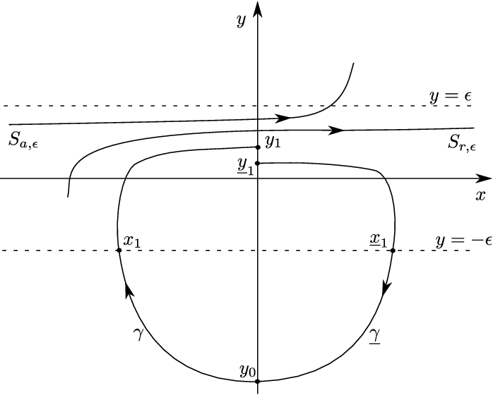
Refer to caption
Figure 13: Important quantities for case V​I3ϵVI_{3}^{\epsilon}, relevant to Proposition 8.51. The region of regularization y∈(−ϵ,ϵ)y\in(-\epsilon,\epsilon) is exaggerated for illustrative purposes.

We consider the distance function:

𝒟⁡(y0,μ2)=y1−y¯1.\displaystyle\mathcal{D}(y_{0},\mu_{2})=y_{1}-\underline{y}_{1}.

Roots of 𝒟\mathcal{D} correspond to periodic orbits. As in [21] we solve 𝒟⁡(y0,μ2)=0\mathcal{D}(y_{0},\mu_{2})=0 by noting, from Fenichel theory, that

𝒟(y0,μ2,c)=𝒪(e−c/ϵ),c=c(y0)>0.\displaystyle\mathcal{D}(y_{0},\mu_{2,c})=\mathcal{O}(e^{-c/\epsilon}),\quad c=c(y_{0})>0.

Since Sr,ϵS_{r,\epsilon} and Sa,ϵS_{a,\epsilon} are transverse for μ2=μ2,c\mu_{2}=\mu_{2,c} this then effectively implies the existence of a μ2=μ2,p​(y0)\mu_{2}=\mu_{2,p}(y_{0}) solving 𝒟⁡(y0,μ2)=0\mathcal{D}(y_{0},\mu_{2})=0 and satisfying μ2,p=μ2,c+𝒪(e−c/ϵ)\mu_{2,p}=\mu_{2,c}+\mathcal{O}(e^{-c/\epsilon}). Since x1x_{1} and x¯1\underline{x}_{1} are increasing functions of y0y_{0} for y0y_{0} small, it also follows that μ2,p​(y0)\mu_{2,p}(y_{0}) approaches μ2,c\mu_{2,c} monotonically as y0y_{0} increases, at least for y0y_{0} sufficiently small. The stability of the periodic orbits is determined by the sign of a way-in/way-out function R=R⁡(y0)R=R(y_{0}), see [21, Proposition 5.4], that measures the contraction and expansion along Sa,rS_{a,r}. In our case the contraction and expansion is determined by the following function

(X2+​(x,0,0)−X2−​(x,0,0))​ϕ′​(y^).\displaystyle(X_{2}^{+}(x,0,0)-X_{2}^{-}(x,0,0))\phi^{\prime}(\hat{y}).

Inserting y^=y^c=ϕ−1​(β−1β+1)\hat{y}=\hat{y}_{c}=\phi^{-1}\left(\frac{\beta-1}{\beta+1}\right) from (67), which corresponds to Sa,rS_{a,r} for μ2=r2=0\mu_{2}=r_{2}=0, we obtain the function R=R⁡(y0)R=R(y_{0}):

R⁡(y0)=ϕ1,c​∫x1​(y0,0)x¯1​(y0,0)(X2+​(x,0,0)−X2−​(x,0,0))​𝑑x.\displaystyle R(y_{0})=\phi_{1,c}\int_{x_{1}(y_{0},0)}^{\underline{x}_{1}(y_{0},0)}(X_{2}^{+}(x,0,0)-X_{2}^{-}(x,0,0))dx.

Since ϕ1,c=ϕ′​(y^c)>0\phi_{1,c}=\phi^{\prime}(\hat{y}_{c})>0, the sign of RR coincides with the sign of

R~​(y0)=∫x1​(y0,0)x¯1​(y0,0)(X2+​(x,0,0)−X2−​(x,0,0))​𝑑x.\displaystyle\tilde{R}(y_{0})=\int_{x_{1}(y_{0},0)}^{\underline{x}_{1}(y_{0},0)}(X_{2}^{+}(x,0,0)-X_{2}^{-}(x,0,0))dx.

We obtain the following proposition:

Proposition 8.51.

Consider a point p=(0,y0)p=(0,y_{0}) with y0∈[−c1−1,−c2−1]y_{0}\in[-c_{1}^{-1},-c_{2}^{-1}] with c2>c1c_{2}>c_{1} sufficiently large but fixed. Then for ϵ≤ϵ0​(c1,c2)\epsilon\leq\epsilon_{0}(c_{1},c_{2}) sufficiently small there exists a unique periodic orbit through pp for μ=μp​(r2,y0)\mu=\mu_{p}(r_{2},y_{0}) where

μp(r2,y0)≡μc+𝒪(e−c/ϵ).\displaystyle\mu_{p}(r_{2},y_{0})\equiv\mu_{c}+\mathcal{O}(e^{-c/\epsilon}).

The function μp​(r2,⋅)\mu_{p}(r_{2},\cdot) is monotonic so that μp​(r2,y0)\mu_{p}(r_{2},y_{0}) approaches μc​(r2)\mu_{c}(r_{2}) as y0y_{0} increases.

The periodic orbits are attracting if

ΔV​I3≡23​α​β​(α⁡(η−+β​η+)+β⁡(β+1)​(ζ−+χ−)),\displaystyle\Delta_{VI_{3}}\equiv\frac{2}{3\alpha\beta}\left(\alpha(\eta^{-}+\beta\eta^{+})+\beta(\beta+1)(\zeta^{-}+\chi^{-})\right), (109)

is negative. They are repelling if ΔV​I3\Delta_{VI_{3}} is positive.

Proof 8.52.

To verify the statement about stability we need to compute R~​(y0)\tilde{R}(y_{0}). To do this we invert x1=x1​(y0,0)x_{1}=x_{1}(y_{0},0) for y0y_{0} and parametrize x¯1\underline{x}_{1} in terms of x1x_{1} rather than y0y_{0}. Then x¯1​(x1)\underline{x}_{1}(x_{1}) is obtained from the map σ0−\sigma_{0}^{-} in Lemma 3.11 with μ=0\mu=0:

x¯1=σ0−​(x1)=−x1+A−​x12+𝒪⁡(x13),\displaystyle\underline{x}_{1}=\sigma_{0}^{-}(x_{1})=-x_{1}+A^{-}x_{1}^{2}+\mathcal{O}(x_{1}^{3}),

using the backward flow of X−X^{-}, where A−A^{-} is given by (26). We therefore consider the following integral

R~​(x1)\displaystyle\tilde{R}(x_{1}) =∫x1x¯1​(x1)(X2+​(x,0,0)−X2−​(x,0,0))​𝑑x\displaystyle=\int_{x_{1}}^{\underline{x}_{1}(x_{1})}(X_{2}^{+}(x,0,0)-X_{2}^{-}(x,0,0))dx
=∫x1x¯1​(x1)((1+β)​x+(η+−η−)​x2+𝒪⁡(x3))​𝑑x\displaystyle=\int_{x_{1}}^{\underline{x}_{1}(x_{1})}((1+\beta)x+(\eta^{+}-\eta^{-})x^{2}+\mathcal{O}(x^{3}))dx
=(A−​(1+β)+23​(η+−η−))​|x1|3+𝒪⁡(x14).\displaystyle=\left(A^{-}(1+\beta)+\frac{2}{3}(\eta^{+}-\eta^{-})\right)|x_{1}|^{3}+\mathcal{O}(x_{1}^{4}).

Hence the sign of R~​(x1)\tilde{R}(x_{1}) is determined by

A−​(1+β)+23​(η+−η−)=23​α​β​(α⁡(η−+β​η+)+β⁡(β+1)​ζ−),\displaystyle A^{-}(1+\beta)+\frac{2}{3}(\eta^{+}-\eta^{-})=\frac{2}{3\alpha\beta}\left(\alpha(\eta^{-}+\beta\eta^{+})+\beta(\beta+1)\zeta^{-}\right),

where we have used (26). The right hand side is (109). Since R~<0\tilde{R}<0 implies stability while R~>0\tilde{R}>0 implies instability the result follows for x1x_{1} (and hence y0y_{0}) sufficiently small.

Remark 8.53.

In classical planar slow-fast systems [21], a canard is generically associated with a Hopf bifurcation and a canard explosion. This is not necessarily the case here. For example the PWS case V​V1VV_{1} has a singular canard but no local limit cycles in either the PWS system or its regularization. Conversely, the regularized system can undergo a Hopf bifurcation without the presence of a canard. This is demonstrated by case I​I2ϵII_{2}^{\epsilon}.

We conclude this subsection with Table 3 which summarizes properties of the seven regularized two-folds (compare with Table 1).

Table 3: 1: type of regularized two-fold singularity. 2: value of α​δ\alpha\delta. 3: equilibrium (x = no, ✓\checkmark = yes). 4: sign of Ω\Omega. 5: Hopf (x = no, ✓\checkmark = yes, n.a. = not applicable). 6: value of β\beta. 7: canard (x = no, ✓\checkmark = yes).
1 2 3 4 5 6 7
Type α​δ\alpha\delta Equilibrium Ω\Omega Hopf β\beta Canard
V​V1ϵVV_{1}^{\epsilon} + x + n.a. + ✓\checkmark
V​V2ϵVV_{2}^{\epsilon} - ✓\checkmark - x - x
V​I1ϵVI_{1}^{\epsilon} + x ±\pm n.a. - x
V​I2ϵVI_{2}^{\epsilon} - ✓\checkmark - x + ✓\checkmark
V​I3ϵVI_{3}^{\epsilon} - ✓\checkmark + ✓\checkmark + ✓\checkmark
I​I1ϵII_{1}^{\epsilon} + x - n.a. + ✓\checkmark
I​I2ϵII_{2}^{\epsilon} - ✓\checkmark + ✓\checkmark - x

8.3 Connecting limit cycles

Having obtained 𝒪⁡(1)\mathcal{O}(1) limit cycles in the two cases I​I2ϵII_{2}^{\epsilon} and V​I3ϵVI_{3}^{\epsilon}, we now analyze the connection between these limit cycles and those described by Proposition 8.46 that are due to the Hopf bifurcation. The results are summarized in one of our main results:

Theorem 8.54.

For ϵ\epsilon sufficiently small:

  • I​I2ϵII_{2}^{\epsilon}:

    There exists a CkC^{k}-smooth family of locally unique periodic orbits of the regularized system (36) that is due to the Hopf bifurcation in Theorem 7.38. If a2<0a_{2}<0 (a2>0a_{2}>0) where a2a_{2} is the first Lyapunov coefficient as defined in (94), then the periodic orbits are attracting (repelling) near the Hopf bifurcation. If

    ΔI​I2=23​α​β​(α⁡(η−+β​η+)+β⁡(ζ−+χ−+α⁡(ζ++χ+))),\displaystyle\Delta_{II_{2}}=\frac{2}{3\alpha\beta}\left(\alpha(\eta^{-}+\beta\eta^{+})+\beta(\zeta^{-}+\chi^{-}+\alpha(\zeta^{+}+\chi^{+}))\right), (29)

    is negative (positive) then the periodic orbits for ΔI​I2−1​μ≤−c​ϵ\Delta_{II_{2}}^{-1}\mu\leq-c\sqrt{\epsilon}, c>0c>0 sufficiently large, are attracting (repelling). The periodic orbits for μ=𝒪⁡(1)\mu=\mathcal{O}(1) (with respect to ϵ\epsilon) are continuously 𝒪⁡(ϵ)\mathcal{O}(\epsilon)-close to the PWS periodic orbits in Proposition 3.13.

  • V​I3ϵVI_{3}^{\epsilon}:

    There exists a CkC^{k}-smooth family of small periodic orbits of the regularized system (36) that is due to the Hopf bifurcation in Theorem 7.38. There also exists a CkC^{k}-smooth family of periodic orbits that are 𝒪⁡(1)\mathcal{O}(1) (with respect to ϵ\epsilon) in amplitude and which undergo a canard explosion, where the amplitude changes by 𝒪⁡(1)\mathcal{O}(1) within an exponentially small parameter regime around the canard value μ=ϵ​μ2,c​(ϵ)\mu=\sqrt{\epsilon}\mu_{2,c}(\sqrt{\epsilon}) (see Theorem 6.29). If a2<0a_{2}<0 (a2>0a_{2}>0) where a2a_{2} is the first Lyapunov coefficient as defined in (94), then the periodic orbits are attracting (repelling) near the Hopf bifurcation. If

    ΔV​I3=23​α​β​(α⁡(η−+β​η+)+β⁡(β+1)​(ζ−+χ−))\displaystyle\Delta_{VI_{3}}=\frac{2}{3\alpha\beta}\left(\alpha(\eta^{-}+\beta\eta^{+})+\beta(\beta+1)(\zeta^{-}+\chi^{-})\right) (109)

    is negative (positive) then the 𝒪⁡(1)\mathcal{O}(1)-periodic orbits are attracting (repelling).

The proof of Theorem 8.54 is divided into two cases: I​I2ϵII_{2}^{\epsilon} and V​I3ϵVI_{3}^{\epsilon}.

8.3.1 Connecting limit cycles for case I​I2ϵII_{2}^{\epsilon} using charts κ1,3\kappa_{1,3}

To connect the periodic orbits described in chart κ2\kappa_{2} by Proposition 8.46 with the 𝒪⁡(1)\mathcal{O}(1) periodic orbits in Proposition 8.49 we first return to the original (x,y)(x,y) variables in which the region of regularization is y∈(−ϵ,ϵ)y\in(-\epsilon,\epsilon) and consider the mappings σϵ±\sigma_{\epsilon}^{\pm} taking (x0,ϵ)(x_{0},\epsilon) to (σϵ+​(x0),ϵ)(\sigma_{\epsilon}^{+}(x_{0}),\epsilon) and (x1,−ϵ)(x_{1},-\epsilon) to (σϵ−​(x1),−ϵ)(\sigma_{\epsilon}^{-}(x_{1}),-\epsilon), respectively. See Fig. 14. We have:

Lemma 8.55.

Fix c>0c>0 large. The maps σϵ±\sigma_{\epsilon}^{\pm} are defined for

x∈(xf+​(μ,ϵ),c−1]\displaystyle x\in(x_{f}^{+}(\mu,\epsilon),c^{-1}] wherexf+​(μ,ϵ)≡−χ+​ϵ+𝒪⁡(ϵ⁡(μ+ϵ)),\displaystyle\quad\text{where}\quad x_{f}^{+}(\mu,\epsilon)\equiv-\chi^{+}\epsilon+\mathcal{O}(\epsilon(\mu+\epsilon)), (110)
and
x∈[−c−1,xf−(μ,ϵ))\displaystyle x\in[-c^{-1},x_{f}^{-}(\mu,\epsilon)) wherexf−​(μ,ϵ)≡μ−β−​χ−​ϵ+𝒪⁡(ϵ⁡(μ+ϵ)),\displaystyle\quad\text{where}\quad x_{f}^{-}(\mu,\epsilon)\equiv\mu-\beta^{-}\chi^{-}\epsilon+\mathcal{O}(\epsilon(\mu+\epsilon)), (111)

respectively and for those xx the maps σϵ±\sigma_{\epsilon}^{\pm} satisfy

σϵ±=σ0±+𝒪⁡(ϵ),\displaystyle\sigma_{\epsilon}^{\pm}=\sigma_{0}^{\pm}+\mathcal{O}(\epsilon), (112)

where σ0±\sigma_{0}^{\pm} are described in Lemma 3.11.

Proof 8.56.

The mappings σ0±\sigma_{0}^{\pm} map {y=0}\{y=0\} to itself by the forward flow of X±X^{\pm} for x>0x>0 and x<μx<\mu, respectively. The mappings σϵ±\sigma_{\epsilon}^{\pm}, on the other hand, map {y=±ϵ}\{y=\pm\epsilon\} to itself by the forward flow of X±X^{\pm}, respectively. Here σϵ+\sigma_{\epsilon}^{+} is defined for x>xf+​(μ,ϵ)x>x_{f}^{+}(\mu,\epsilon) where X2+​(xf+​(μ,ϵ),ϵ,μ)=0X_{2}^{+}(x_{f}^{+}(\mu,\epsilon),\epsilon,\mu)=0 while σϵ+\sigma_{\epsilon}^{+} is defined for x<xf−​(μ,ϵ)x<x_{f}^{-}(\mu,\epsilon) where X2−​(xf−​(μ,ϵ),−ϵ,μ)=0X_{2}^{-}(x_{f}^{-}(\mu,\epsilon),-\epsilon,\mu)=0. Using (15) and (16) and the implicit function theorem gives (110) and (111), respectively, for cc sufficiently large. Equation (112) therefore follows by standard regular perturbation theory.

Remark 8.57.

The mappings σϵ±\sigma_{\epsilon}^{\pm} do not depend upon the regularization. They are due to (37) determined by X±X^{\pm}.

Refer to caption
Figure 14: The mappings σϵ±\sigma_{\epsilon}^{\pm} associated with the regularization of the invisible two-fold singularity I​I2II_{2}, where δ=−1\delta=-1, α>0\alpha>0 and β<0\beta<0. The points (x,y)=(x±,±ϵ)(x,y)=(x^{\pm},\pm\epsilon) are points where X2±​(x,±ϵ,μ)=0X_{2}^{\pm}(x,\pm\epsilon,\mu)=0. Note that the mappings ξ1−\xi_{1}^{-} and ξ3+\xi_{3}^{+} in (114) and (115) describe the fast transitions indicated in the figure by the triple-headed arrows, using the charts κ1\kappa_{1} and κ3\kappa_{3}. These transitions would appear nearly vertical in the stretched coordinate system (x,y^)(x,\hat{y}).

We now write these mappings σϵ∓\sigma_{\epsilon}^{\mp} in terms of the charts κ1,3\kappa_{1,3}. The resulting mappings will be denoted by

σ31−=κ3∘σϵ−∘κ1−1,\displaystyle\sigma_{31}^{-}=\kappa_{3}\circ\sigma_{\epsilon}^{-}\circ\kappa_{1}^{-1},

and

σ13+=κ1∘σϵ−∘κ3−1,\displaystyle\sigma_{13}^{+}=\kappa_{1}\circ\sigma_{\epsilon}^{-}\circ\kappa_{3}^{-1},

respectively, using the subscripts to highlight that these mappings are from κ1\kappa_{1} (κ3\kappa_{3}) to κ3\kappa_{3} (κ1\kappa_{1}), respectively.

Lemma 8.58.

Consider (99). In terms of the charts κ1,3\kappa_{1,3} the mappings σϵ∓\sigma_{\epsilon}^{\mp} take the following forms:

σ31−:κ1∩{y^=−1}\displaystyle\sigma_{31}^{-}:\quad\kappa_{1}\cap\{\hat{y}=-1\} →κ3∩{y^=−1},\displaystyle\rightarrow\kappa_{3}\cap\{\hat{y}=-1\},
r3\displaystyle r_{3} =r1​(1+2​μ1+A−​r1+𝒪⁡(r1​(ϵ1+μ1+r1))CLOSE,\displaystyle=r_{1}(1+2\mu_{1}+A^{-}r_{1}+\mathcal{O}(r_{1}(\epsilon_{1}+\mu_{1}+r_{1})),
ϵ3\displaystyle\epsilon_{3} =ϵ1​(1−2​(2​μ1+A−​r1)+𝒪⁡(r1​(ϵ1+μ1+r1)+μ12)),\displaystyle=\epsilon_{1}(1-2(2\mu_{1}+A^{-}r_{1})+\mathcal{O}(r_{1}(\epsilon_{1}+\mu_{1}+r_{1})+\mu_{1}^{2})),
μ3\displaystyle\mu_{3} =μ1​(1−(2​μ1+A−​r1)+𝒪⁡(r1​(ϵ1+μ1+r1)+μ12)),\displaystyle=\mu_{1}(1-(2\mu_{1}+A^{-}r_{1})+\mathcal{O}(r_{1}(\epsilon_{1}+\mu_{1}+r_{1})+\mu_{1}^{2})),

and

σ13+:κ3∩{y^=1}\displaystyle\sigma_{13}^{+}:\quad\kappa_{3}\cap\{\hat{y}=1\} →κ1∩{y^=1},\displaystyle\rightarrow\kappa_{1}\cap\{\hat{y}=1\},
r1\displaystyle r_{1} =r3​(1−A+​r3+𝒪⁡(r3​(ϵ3+μ3+r3))CLOSE,\displaystyle=r_{3}(1-A^{+}r_{3}+\mathcal{O}(r_{3}(\epsilon_{3}+\mu_{3}+r_{3})),
ϵ1\displaystyle\epsilon_{1} =ϵ3​(1+2​A+​r3+𝒪⁡(r3​(ϵ3+μ3+r3))),\displaystyle=\epsilon_{3}(1+2A^{+}r_{3}+\mathcal{O}(r_{3}(\epsilon_{3}+\mu_{3}+r_{3}))),
μ1\displaystyle\mu_{1} =μ3​(1+A+​r3+𝒪⁡(r3​(ϵ3+μ3+r3))),\displaystyle=\mu_{3}(1+A^{+}r_{3}+\mathcal{O}(r_{3}(\epsilon_{3}+\mu_{3}+r_{3}))),

respectively, for r1r_{1}, ϵ1\epsilon_{1} and μ1\mu_{1} sufficiently small.

Proof 8.59.

Consider the case σϵ−\sigma_{\epsilon}^{-} (the case σϵ+\sigma_{\epsilon}^{+} is identical). We then use (112) and Lemma 3.11 and set x1=−r1x_{1}=-r_{1} and x3=r3x_{3}=r_{3} as described by the charts κ1,3\kappa_{1,3}, respectively. The expressions for ϵ3\epsilon_{3} and μ3\mu_{3} then follow from the conservation of ϵ\epsilon and μ\mu, respectively. The condition (110) and (111) are satisfied for r3r_{3}, ϵ3\epsilon_{3}, μ3\mu_{3} and r1r_{1} ϵ1\epsilon_{1}, μ1\mu_{1}, respectively, sufficiently small.

We then consider the Poincaré mapping PϵP_{\epsilon} from (108) used in Proposition 8.49 and write this mapping in chart κ3\kappa_{3}. The resulting mapping is given by

P3=κ3∘Pϵ∘κ3−1:κ3∩{y^=1}\displaystyle P_{3}=\kappa_{3}\circ P_{\epsilon}\circ\kappa_{3}^{-1}:\quad\kappa_{3}\cap\{\hat{y}=1\} →κ3∩{y^=1},\displaystyle\rightarrow\kappa_{3}\cap\{\hat{y}=1\}, (113)
(r3,ϵ3,μ3)\displaystyle(r_{3},\epsilon_{3},\mu_{3}) ↦(r3+,ϵ3+,μ3+),\displaystyle\mapsto(r_{3}^{+},\epsilon_{3}^{+},\mu_{3}^{+}),

We will compose P3P_{3} into four different mappings σ13+\sigma_{13}^{+}, ξ1−\xi_{1}^{-}, σ31−\sigma_{31}^{-} and ξ3+\xi_{3}^{+} so that:

P3=ξ3+∘σ31−∘ξ1−∘σ13+.P_{3}=\xi_{3}^{+}\circ\sigma_{31}^{-}\circ\xi_{1}^{-}\circ\sigma_{13}^{+}.

The mappings σ13+\sigma_{13}^{+} and σ31−\sigma_{31}^{-} are described in Lemma 8.58 while ξ1−\xi_{1}^{-} and ξ3+\xi_{3}^{+} are given in terms of the forward flow associated with the differential equations in charts κ1\kappa_{1} and κ3\kappa_{3} (see (70) and (72)) and map {y=±ϵ}\{y=\pm\epsilon\} ({y^=±1}\{\hat{y}=\pm 1\}) to {y=∓ϵ}\{y=\mp\epsilon\} ({y^=∓1}\{\hat{y}=\mp 1\}), respectively. Hence the mappings:

ξ1−:{y^=1}\displaystyle\xi_{1}^{-}:\{\hat{y}=1\} →{y^=−1},\displaystyle\rightarrow\{\hat{y}=-1\}, (114)
(r1,ϵ1,μ1)\displaystyle(r_{1},\epsilon_{1},\mu_{1}) ↦(r1−,ϵ1−,μ1−),\displaystyle\mapsto(r_{1}^{-},\epsilon_{1}^{-},\mu_{1}^{-}),

and

ξ3+:{y^=−1}\displaystyle\xi_{3}^{+}:\{\hat{y}=-1\} →{y^=1},\displaystyle\rightarrow\{\hat{y}=1\}, (115)
(r3,ϵ3,μ3)\displaystyle(r_{3},\epsilon_{3},\mu_{3}) ↦(r3+,ϵ3+,μ3+),\displaystyle\mapsto(r_{3}^{+},\epsilon_{3}^{+},\mu_{3}^{+}),

are defined by the forward flow of the following equations:

r˙1\displaystyle\dot{r}_{1} =−r1​ϵ1​F~1​(r1,y^,ϵ1,μ1),\displaystyle=-r_{1}\epsilon_{1}\tilde{F}_{1}(r_{1},\hat{y},\epsilon_{1},\mu_{1}), (116)
y^˙\displaystyle\dot{\hat{y}} =(−1+𝒪⁡(r1))​(1+ϕ⁡(y^))+(β⁡(1+μ1)+𝒪⁡(r1))​(1−ϕ⁡(y^)),\displaystyle=(-1+\mathcal{O}(r_{1}))(1+\phi(\hat{y}))+(\beta(1+\mu_{1})+\mathcal{O}(r_{1}))(1-\phi(\hat{y})),
ϵ˙1\displaystyle\dot{\epsilon}_{1} =2​ϵ12​F~1​(r1,y^,ϵ1,μ1),\displaystyle=2\epsilon_{1}^{2}\tilde{F}_{1}(r_{1},\hat{y},\epsilon_{1},\mu_{1}),
μ˙1\displaystyle\dot{\mu}_{1} =ϵ1​μ1​F~1​(r1,y^,ϵ1,μ1),\displaystyle=\epsilon_{1}\mu_{1}\tilde{F}_{1}(r_{1},\hat{y},\epsilon_{1},\mu_{1}),

and

r˙3\displaystyle\dot{r}_{3} =r3​ϵ3​F~3​(r3,y^,ϵ3,μ3),\displaystyle=r_{3}\epsilon_{3}\tilde{F}_{3}(r_{3},\hat{y},\epsilon_{3},\mu_{3}),
y^˙\displaystyle\dot{\hat{y}} OPEN=(1+𝒪⁡(r3))​(1+ϕ⁡(y^))+(−β⁡(1−μ3)+𝒪⁡(r3))​(1−ϕ⁡(y^))),\displaystyle=(1+\mathcal{O}(r_{3}))(1+\phi(\hat{y}))+(-\beta(1-\mu_{3})+\mathcal{O}(r_{3}))(1-\phi(\hat{y}))),
ϵ˙3\displaystyle\dot{\epsilon}_{3} =−2​ϵ32​F~3​(r3,y^,ϵ3,μ3),\displaystyle=-2\epsilon_{3}^{2}\tilde{F}_{3}(r_{3},\hat{y},\epsilon_{3},\mu_{3}),
μ˙3\displaystyle\dot{\mu}_{3} =−ϵ3​μ3​F~3​(r3,y^,ϵ3,μ3),\displaystyle=-\epsilon_{3}\mu_{3}\tilde{F}_{3}(r_{3},\hat{y},\epsilon_{3},\mu_{3}),

respectively. These equations are equations (70) and (72), respectively, written in terms of y^\hat{y} rather than ww, where

F~1​(r1,y^,ϵ1,μ1)\displaystyle\tilde{F}_{1}(r_{1},\hat{y},\epsilon_{1},\mu_{1}) =(−1+𝒪⁡(r1))​(1+ϕ⁡(y^))+(α+𝒪⁡(r1))​(1−ϕ⁡(y^)),\displaystyle=(-1+\mathcal{O}(r_{1}))(1+\phi(\hat{y}))+(\alpha+\mathcal{O}(r_{1}))(1-\phi(\hat{y})),
F~3​(r3,y^,ϵ3,μ3)\displaystyle\tilde{F}_{3}(r_{3},\hat{y},\epsilon_{3},\mu_{3}) =(−1+𝒪⁡(r3))​(1+ϕ⁡(y^))+(α+𝒪⁡(r3))​(1−ϕ⁡(y^)).\displaystyle=(-1+\mathcal{O}(r_{3}))(1+\phi(\hat{y}))+(\alpha+\mathcal{O}(r_{3}))(1-\phi(\hat{y})).
Lemma 8.60.

Consider (99) and let

E\displaystyle E =∫−11−(1+ϕ⁡(y^))+α⁡(1−ϕ⁡(y^))1+ϕ⁡(y^)−β⁡(1−ϕ⁡(y^))​𝑑y^.\displaystyle=\int_{-1}^{1}\frac{-(1+\phi(\hat{y}))+\alpha(1-\phi(\hat{y}))}{1+\phi(\hat{y})-\beta(1-\phi(\hat{y}))}d\hat{y}.

Then the mappings ξ1−\xi_{1}^{-}, ξ3+\xi_{3}^{+} in (114) and (115) take the following form:

ξ1−:r1−\displaystyle\xi_{1}^{-}:\,r_{1}^{-} =r1​(1−E​ϵ1+𝒪⁡(r1​ϵ1)),\displaystyle=r_{1}(1-E\epsilon_{1}+\mathcal{O}(r_{1}\epsilon_{1})),
ϵ1−\displaystyle\epsilon_{1}^{-} =ϵ1​(1+2​E​ϵ1+𝒪⁡(r1​ϵ1)),\displaystyle=\epsilon_{1}(1+2E\epsilon_{1}+\mathcal{O}(r_{1}\epsilon_{1})),
μ1−\displaystyle\mu_{1}^{-} =μ1​(1+E​ϵ1+𝒪⁡(r1​ϵ1)),\displaystyle=\mu_{1}(1+E\epsilon_{1}+\mathcal{O}(r_{1}\epsilon_{1})),

and

ξ3+:r3+\displaystyle\xi_{3}^{+}:\,r_{3}^{+} =r3​(1+E​ϵ3+𝒪⁡(r3​ϵ3)),\displaystyle=r_{3}(1+E\epsilon_{3}+\mathcal{O}(r_{3}\epsilon_{3})),
ϵ3+\displaystyle\epsilon_{3}^{+} =ϵ3​(1−2​E​ϵ3+𝒪⁡(r3​ϵ3)),\displaystyle=\epsilon_{3}(1-2E\epsilon_{3}+\mathcal{O}(r_{3}\epsilon_{3})),
μ3+\displaystyle\mu_{3}^{+} =μ3​(1−E​ϵ3+𝒪⁡(r3​ϵ3)).\displaystyle=\mu_{3}(1-E\epsilon_{3}+\mathcal{O}(r_{3}\epsilon_{3})).
Proof 8.61.

Consider ξ1−\xi_{1}^{-} and (116) (the analysis for ξ3+\xi_{3}^{+} is identical). Since β<0\beta<0 we have that y^˙<0\dot{\hat{y}}<0 for y^∈[−1,1]\hat{y}\in[-1,1] for r1=μ1=0r_{1}=\mu_{1}=0 and hence we can replace time by y^\hat{y} by dividing the equations for r˙1\dot{r}_{1}, ϵ˙1\dot{\epsilon}_{1} and μ˙1\dot{\mu}_{1} by y^˙\dot{\hat{y}}. The point (r1,ϵ1,μ1)=0(r_{1},\epsilon_{1},\mu_{1})=0 is a fixed point of these equations. Solving the second order variational equations gives the desired result.

We then have:

Lemma 8.62.

Consider (99). The Poincaré map P3:(r3,ϵ3,μ3)↦(r3+,ϵ3+,μ3+)P_{3}:\,(r_{3},\epsilon_{3},\mu_{3})\mapsto(r_{3}^{+},\epsilon_{3}^{+},\mu_{3}^{+}) takes the following form:

P3:r3+\displaystyle P_{3}:\,r_{3}^{+} =r3​(1+2​μ3+ΔI​I2​r3+𝒪⁡(r3​(ϵ3+μ3+r3))CLOSE,\displaystyle=r_{3}(1+2\mu_{3}+\Delta_{II_{2}}r_{3}+\mathcal{O}(r_{3}(\epsilon_{3}+\mu_{3}+r_{3})), (118)
ϵ3+\displaystyle\epsilon_{3}^{+} =ϵ3​(1−2​(2​μ3+ΔI​I2​r3)+𝒪⁡(r3​(ϵ3+μ3+r3))CLOSE,\displaystyle=\epsilon_{3}(1-2(2\mu_{3}+\Delta_{II_{2}}r_{3})+\mathcal{O}(r_{3}(\epsilon_{3}+\mu_{3}+r_{3})),
μ3+\displaystyle\mu_{3}^{+} =μ3​(1−(2​μ3+ΔI​I2​r3)+𝒪⁡(r3​(ϵ3+μ3+r3))CLOSE,\displaystyle=\mu_{3}(1-(2\mu_{3}+\Delta_{II_{2}}r_{3})+\mathcal{O}(r_{3}(\epsilon_{3}+\mu_{3}+r_{3})),

where ΔI​I2\Delta_{II_{2}} is given by (29).

Proof 8.63.

We use Lemma 8.60 and Lemma 8.58.

Remark 8.64.

Note that to leading order (118) is independent of EE and hence of ϕ\phi, the regularization function. Hence ϕ\phi does not induce bifurcations in the transition from sufficiently large limit cycles (meaning ν\nu sufficiently small) in chart κ2\kappa_{2} to the 𝒪⁡(1)\mathcal{O}(1) limit cycles.

Next, we solve for fixed points of P3P_{3} and obtain:

Proposition 8.65.

Suppose that ΔI​I2\Delta_{II_{2}} in (29) is non-zero. Then for μ3,ϵ3\mu_{3},\,\epsilon_{3} sufficiently small and μ3​ΔI​I2−1<0\mu_{3}\Delta_{II_{2}}^{-1}<0, the mapping P3P_{3} has a locally unique family of fixed points:

r3\displaystyle r_{3} =−2​μ3​ΔI​I2−1+𝒪⁡(μ3​(ϵ3+μ3)).\displaystyle=-2\mu_{3}\Delta_{II_{2}}^{-1}+\mathcal{O}(\mu_{3}(\epsilon_{3}+\mu_{3})). (119)

The family of fixed point of P3P_{3} corresponds to a CkC^{k}-smooth family of periodic orbits which are attracting (repelling) for ΔI​I2<0\Delta_{II_{2}}<0 (ΔI​I2>0\Delta_{II_{2}}>0).

Proof 8.66.

Suppose that (r3,μ3,ϵ3)(r_{3},\mu_{3},\epsilon_{3}) is a fixed point of P3P_{3}. Then since μ=r3​μ3\mu=r_{3}\mu_{3} and ϵ=r3​ϵ3\epsilon=r_{3}\epsilon_{3} we solve for r3=r3​(μ3,ϵ3)r_{3}=r_{3}(\mu_{3},\epsilon_{3}) by setting r3+=r3r_{3}^{+}=r_{3} in (118). This gives

2​μ3+ΔI​I2​r3+𝒪⁡(r3​(ϵ3+μ3+r3))=0.\displaystyle 2\mu_{3}+\Delta_{II_{2}}r_{3}+\mathcal{O}(r_{3}(\epsilon_{3}+\mu_{3}+r_{3}))=0.

We solve this equation by the implicit function theorem and obtain (119). The statement about stability follows from the fact that the sign of ΔI​I2\Delta_{II_{2}} determines the sign of ∂r3r3+=r3​(ΔI​I2+𝒪⁡(ϵ3+μ3+r3))\partial_{r_{3}}r_{3}^{+}=r_{3}(\Delta_{II_{2}}+\mathcal{O}(\epsilon_{3}+\mu_{3}+r_{3})).

The periodic orbits in chart κ2\kappa_{2}, described by Proposition 8.46, that are due to the Hopf bifurcation, are locally unique since they are obtained by the implicit function theorem for μ2=r2=0\mu_{2}=r_{2}=0. These orbits can be continued all the way up to the section Λ2+\Lambda_{2}^{+}, defined in (68) (see also Remark 8.48). The periodic orbits that are 𝒪⁡(1)\mathcal{O}(1) with respect to 𝒪⁡(ϵ)\mathcal{O}(\epsilon), described by Proposition 8.49, are also locally unique by virtue of the implicit function theorem. Therefore by setting ϵ3=ν2\epsilon_{3}=\nu^{2}, corresponding to the section Λ2+\Lambda_{2}^{+} (68), and taking ν\nu sufficiently small, we obtain:

x2=ν−1,y^=1,μ2=−ΔI​I22​ν2​r2+𝒪⁡(r22),\displaystyle x_{2}=\nu^{-1},\,\hat{y}=1,\,\mu_{2}=-\frac{\Delta_{II_{2}}}{2\nu^{2}}r_{2}+\mathcal{O}(r_{2}^{2}), (120)

using (64) and (119). Therefore we can conclude that the periodic orbits described by (119) coincide with the locally unique ones in chart κ2\kappa_{2} described by Proposition 8.46. Similarly, setting r3=ρr_{3}=\rho, corresponding to section Λ+\Lambda^{+} (52), shows that the periodic orbits in (119) coincide with those in Proposition 8.49, where these are defined. This gives a CkC^{k}-smooth and locally unique family of periodic orbits as described by Theorem 8.54, case I​I2ϵII_{2}^{\epsilon}.

Remark 8.67.

We believe that the application of the directional charts κ1,3\kappa_{1,3} in this section to describe the Poincaré-mapping PϵP_{\epsilon} is a novelty. The coordinates of κ1,3\kappa_{1,3} enabled us to connect the periodic orbits in chart κ2\kappa_{2} with the larger periodic orbits without the need for careful estimation. This is a general advantage of the blowup method and the phase directional charts κ1,3\kappa_{1,3}. Having said that, it might be possible to prove the connection of the limit cycles in κ2\kappa_{2} with the larger limit cycles in Proposition 8.49 by working in chart κ2\kappa_{2} alone. To do this one would, however, have to perform a careful estimation of the function DD in (102). The following remark, Remark 8.68, contains a discussion of this issue.

Remark 8.68.

By (64) it follows that the family of fixed points of P3P_{3} described in Proposition 8.65 intersects Λ2+\Lambda_{2}^{+} in (120). By Theorem 8.54, case I​I2ϵII_{2}^{\epsilon}, this fixed point of P3P_{3} corresponds to a periodic orbit obtained from Proposition 8.46 for a corresponding value of the energy constant hh. Hence the value of μ2\mu_{2} in (120) must agree with the value given in (107). This is a corollary of Theorem 8.54, case I​I2ϵII_{2}^{\epsilon}. One may expect that there could be a more direct way of showing this. We now outline a formal derivation of the result by approximation the integrals in Dr2D_{r_{2}} and Dμ2D_{\mu_{2}} in (107).

Since x2=ν−1x_{2}=\nu^{-1} in (120) we take h=12​ν2h=\frac{1}{2\nu^{2}}. To compute Dr2D_{r_{2}} (104) we first substitute d​t=((1+ϕ)−β⁡(1−ϕ))​x2​d​ydt=((1+\phi)-\beta(1-\phi))x_{2}dy and integrate from y^0h\hat{y}_{0}^{h} to y^1h\hat{y}_{1}^{h}. We then split this integration into (a) an integration from y^=y^0h\hat{y}=\hat{y}_{0}^{h} to y^=0\hat{y}=0 and (b) an integration from y^=0\hat{y}=0 to y^=y^0h\hat{y}=\hat{y}_{0}^{h}. We then ignore the contribution from the region of regularization and simply set ϕ=∓1\phi=\mp 1 in the integrations (a) and (b), respectively. We apply the same approximation to the Hamiltonian H⁡(x2,y^)H(x_{2},\hat{y}) and obtain the value of y^0h\hat{y}_{0}^{h} and y^1h\hat{y}_{1}^{h} from the equation H⁡(0,y^)=hH(0,\hat{y})=h. Combining this gives the following approximation of Dr2D_{r_{2}}:

Dr2≈23​ν3​β​α​(α⁡(η−+β​η+)+β⁡(ζ−+χ−+α⁡(ζ++χ+))),\displaystyle D_{r_{2}}\approx\frac{2}{3\nu^{3}\beta\alpha}\left(\alpha(\eta^{-}+\beta\eta^{+})+\beta(\zeta^{-}+\chi^{-}+\alpha(\zeta^{+}+\chi^{+}))\right),

which is valid for ν\nu small. Hence

Dr2≈ΔI​I2ν3,\displaystyle D_{r_{2}}\approx\frac{\Delta_{II_{2}}}{\nu^{3}},

from (29). For Dμ2D_{\mu_{2}}, as defined in (105), we use (106) and approximate x2x_{2} by the constant value ν−1\nu^{-1}. This gives

Dμ2≈2ν.\displaystyle D_{\mu_{2}}\approx\frac{2}{\nu}.

Hence, from (107), we have

μ2≈−ΔI​I22​ν2​r2,\displaystyle\mu_{2}\approx-\frac{\Delta_{II_{2}}}{2\nu^{2}}r_{2},

which agrees with (120). We have not pursued a rigorous result of this kind.

8.3.2 Connecting limit cycles for case V​I3ϵVI_{3}^{\epsilon}

Krupa and Szmolyan [21] describe the classical canard explosion phenomenon, as observed in the van der Pol system. They prove that the periodic orbits within their chart κ2\kappa_{2} belong to a smooth and unique family of local periodic orbits that also includes 𝒪⁡(1)\mathcal{O}(1) periodic orbits that arise from their canard explosion. Their proof involves careful estimation on the dependency of the function D⁡(r2,μ2,h)D(r_{2},\mu_{2},h), as defined in (102), on the distance to the singular canard (measured by the energy constant hh). It seems plausible that a similar analysis could be performed to our system. However, the situation here is complicated by the fact that our Hamiltonian function HH depends non-trivially on the regularization function ϕ\phi. The statements in Theorem 8.54, case V​I3ϵVI_{3}^{\epsilon}, therefore summarize the previous results in Proposition 8.46 and Proposition 8.51. Instead we conjecture on the connection of small periodic orbits in Proposition 8.46 with the larger ones in Proposition 8.51 as follows:

Conjecture 1.

The two families of periodic orbits in V​I3ϵVI_{3}^{\epsilon} belong to the same family of locally unique periodic orbits.

The limit cycles in Proposition 8.46 and Proposition 8.51 do not seem to be present in the PWS case V​I3VI_{3}.

8.4 Saddle-node bifurcation

We conclude this section with the following main result

Theorem 8.69.

Suppose (98) and (57). Then for ϵ\epsilon sufficiently small:

  • I​I2ϵII_{2}^{\epsilon}:

    There exists an open set of regularization functions such that the periodic orbits in Theorem 8.54, case I​I2ϵII_{2}^{\epsilon}, undergo at least one saddle-node bifurcation.

  • V​I3ϵVI_{3}^{\epsilon}:

    Suppose, in addition, that Conjecture 1 holds. Then there exists an open set of regularization functions such that the periodic orbits in Theorem 8.54, case V​I3ϵVI_{3}^{\epsilon}, undergo at least one saddle-node bifurcation.

Proof 8.70.

A corollary of Theorem 7.39 is that we can always achieve a2​ΔI​I2<0a_{2}\Delta_{II_{2}}<0 or a2​ΔV​I3<0a_{2}\Delta_{VI_{3}}<0. The result therefore follows from the statements in Theorem 8.54 and Conjecture 1.

9 Numerics

In this section we illustrate the results in Theorem 8.69, and provide further support for Conjecture 1, by computing limit cycles for two model systems, for cases I​I2ϵII_{2}^{\epsilon} and V​I3ϵVI_{3}^{\epsilon}.

9.1 Case I​I2ϵII_{2}^{\epsilon}

In this section we consider the regularization of the following model system for case I​I2II_{2}:

X+​(x,y)=(−1−7​xx+2​x2),X−​(x,y,μ)=(1−6​x(x−μ)−2​(x−μ)2),\displaystyle X^{+}(x,y)=\begin{pmatrix}-1-7x\\ x+2x^{2}\end{pmatrix},\quad X^{-}(x,y,\mu)=\begin{pmatrix}1-6x\\ (x-\mu)-2(x-\mu)^{2}\end{pmatrix}, (121)

corresponding to the following parameters:

δ=−1,α=1,β=−1,ζ+=−7,ζ−=−6,η±=±2,χ±=0,Ω=2,\displaystyle\delta=-1,\,\alpha=1,\,\beta=-1,\,\zeta^{+}=-7,\,\zeta^{-}=-6,\,\eta^{\pm}=\pm 2,\,\chi^{\pm}=0,\,\Omega=2,

in (15) and (16). The constant ΔI​I2\Delta_{II_{2}} given in (29) takes the value:

ΔI​I2=−6.\displaystyle\Delta_{II_{2}}=-6.

According to Proposition 3.13 the limit cycles of the PWS system are therefore all stable. According to Theorem 8.54 the 𝒪⁡(1)\mathcal{O}(1) (with respect to ϵ\epsilon) limit cycles of the regularized system are also stable.

We consider two regularization functions77 7 The superscripts ll and cc refer to linear and cubic, respectively.:

ϕl​(y^)=y^fory^∈(−1,1),\displaystyle\phi^{l}(\hat{y})=\hat{y}\quad\text{for}\quad\hat{y}\in(-1,1), (122)

and

ϕc​(y^)=32​y^−12​y^3fory^∈(−1,1).\displaystyle\phi^{c}(\hat{y})=\frac{3}{2}\hat{y}-\frac{1}{2}\hat{y}^{3}\quad\text{for}\quad\hat{y}\in(-1,1). (123)

From (92) we obtain y^0∗=0\hat{y}_{0}^{*}=0 in both cases. Inserting the corresponding values of ϕ1,H=ϕ′​(0),ϕ2,H=ϕ′′​(0)=0,ϕ3,H=ϕ(3)​(0)\phi_{1,H}=\phi^{\prime}(0),\,\phi_{2,H}=\phi^{\prime\prime}(0)=0,\,\phi_{3,H}=\phi^{(3)}(0) into (93) and (94) gives the following values for μ2,H\mu_{2,H} and a2a_{2}:

μ2,Hl\displaystyle\mu_{2,H}^{l} =13​r2+𝒪⁡(r22),\displaystyle=13r_{2}+\mathcal{O}(r_{2}^{2}), (124)
a2l\displaystyle a_{2}^{l} =12,\displaystyle=\frac{1}{2},
μ2,Hc\displaystyle\mu_{2,H}^{c} =263​r2+𝒪⁡(r22)=(8+23)​r2+𝒪⁡(r22),\displaystyle=\frac{26}{3}r_{2}+\mathcal{O}(r_{2}^{2})=(8+\frac{2}{3})r_{2}+\mathcal{O}(r_{2}^{2}),
a2c\displaystyle a_{2}^{c} =−12.\displaystyle=-\frac{1}{2}.

Since a2l​ΔI​I2<0a_{2}^{l}\Delta_{II_{2}}<0 we have from Theorem 8.69 that the linear regularization function (122) introduces a saddle-node bifurcation. We demonstrate this as follows.

Using the numerical bifurcation software AUTO we continued the periodic orbits in the two regularizations of I​I2II_{2}. In Fig. 15 we show the amplitude (measured as max⁡(y^)\max(\hat{y})) of the periodic orbits as a function of the parameter μ2\mu_{2} for r2=ϵ=0.01r_{2}=\sqrt{\epsilon}=0.01. The full line shows the result of using ϕl\phi_{l}, as given in (122), while the dotted line shows the result of using ϕc\phi_{c}, as given in (123). The linear regularization function introduces a saddle-node bifurcation, in agreement with Theorem 8.69. On the other hand, the cubic regularization function does not introduce any saddle-node bifurcation.

The Hopf bifurcations were numerically found to occur at

μ2,Hl≈0.1298,μ2,Hc≈0.0866,\displaystyle\mu_{2,H}^{l}\approx 0.1298,\quad\mu_{2,H}^{c}\approx 0.0866,

which are in good agreement with (124) for r2=0.01r_{2}=0.01. Also, in agreement with Proposition 8.49, we observed that the two family of limit cycles agree for larger values of μ2\mu_{2} since the limit cycles for both regularizations must be 𝒪⁡(ϵ)\mathcal{O}(\epsilon)-close to the limit cycles of the PWS system for μ=𝒪⁡(1)\mu=\mathcal{O}(1).

Refer to caption
Figure 15: Periodic orbit amplitudes as a function of the parameter μ2\mu_{2} for r2=0.01r_{2}=0.01. The full line shows the result of using the linear regularization function (122), the dotted line shows the result of using the cubic regularization function (123). As can be seen, the linear regularization function induces a saddle-node (SN) bifurcation, in agreement with Theorem 8.69.
Remark 9.71.

We obtained system (121) by fixing (122) and (123) and the parameters δ,α,β\delta,\,\alpha,\beta and solving a2l=−a2ca_{2}^{l}=-a_{2}^{c} for ζ±\zeta^{\pm} and η±\eta^{\pm} setting χ±=0\chi^{\pm}=0 for simplicity.

9.2 Case V​I3ϵVI_{3}^{\epsilon}

In this section we consider the following model system for the case V​I3VI_{3}:

X+=(1+12​xx−x3),X−=(−1−2​(x−μ)+(x−μ)2).\displaystyle X^{+}=\begin{pmatrix}1+\frac{1}{2}x\\ x-x^{3}\end{pmatrix},\quad X^{-}=\begin{pmatrix}-1\\ -2(x-\mu)+(x-\mu)^{2}\end{pmatrix}. (125)

Here

δ=1,α=−1,β=2,ζ+=12,ζ−=0,η+=0,η−=1,χ±=0,Ω=1.\displaystyle\delta=1,\,\alpha=-1,\,\beta=2,\,\zeta^{+}=\frac{1}{2},\,\zeta^{-}=0,\,\eta^{+}=0,\,\eta^{-}=1,\,\chi^{\pm}=0,\,\Omega=1.

We sketch the PWS system in Fig. 16 for μ=0\mu=0. It is very similar to Fig. 12 in [22]. However, as opposed to [22] we have included the cubic term in X+X^{+} which gives rise to an invisible tangency at (x,y)=(1,0)(x,y)=(1,0) and a return mechanism from Σ+\Sigma^{+} to Σ−\Sigma^{-}.

Refer to caption
Figure 16: Sketch of the PWS system (125) for μ=0\mu=0. The triple-headed arrows within Σ\Sigma indicate the direction of the sliding vector field.

We then regularize XX in (125) using the cubic function in (123). Since Ω=1>0\Omega=1>0, we can apply Proposition 7.35 to the regularized system and conclude that the system has an equilibrium (90) which undergoes a Hopf bifurcation at

μ2=μ2,Hc≡−112​r2+𝒪⁡(r22).\displaystyle\mu_{2}=\mu_{2,H}^{c}\equiv-\frac{1}{12}r_{2}+\mathcal{O}(r_{2}^{2}). (126)

The first Lyapunov coefficient is obtained from (94):

a\displaystyle a =−564​r2+𝒪⁡(r22).\displaystyle=-\frac{5}{64}r_{2}+\mathcal{O}(r_{2}^{2}). (127)

Since a2c≡−564<0a_{2}^{c}\equiv-\frac{5}{64}<0 we conclude that the periodic orbits are attracting for r2r_{2} (and hence ϵ\epsilon) sufficiently small and appear for μ2>μ2,Hc\mu_{2}>\mu_{2,H}^{c}.

This example also has a maximal canard (see Theorem 6.29). The parameter value at which it occurs is, from (79), given by

μ2,cc\displaystyle\mu_{2,c}^{c} =−19​ϕ1,c​r2+𝒪⁡(r22)≈−0.07806​r2+𝒪⁡(r22),\displaystyle=-\frac{1}{9\phi_{1,c}}r_{2}+\mathcal{O}(r_{2}^{2})\approx-0.07806r_{2}+\mathcal{O}(r_{2}^{2}), (128)

In the last expression we have used (67) to obtain

ϕ1,c≈1.4233.\displaystyle\phi_{1,c}\approx 1.4233.

There is a related example for the case V​I3VI_{3} in [22] on p. 2169 (after reversing time and reflecting x↦−xx\mapsto-x) with the same values of δ\delta, α\alpha and β\beta. The system in [22] has ζ±=∓1\zeta^{\pm}=\mp 1 as the only non-zero coefficients in (14). The reason for modifying the system given in [22] is that their system gives a2=0a_{2}=0 from (94), for all regularization functions ϕ\phi. In fact a detailed calculation shows that a≡0a\equiv 0. The example in [22] is therefore codimension two for the regularization.

In Fig. 17 we have used the numerical bifurcation software AUTO to track the amplitudes of the limit cycles of (125) emanating from the equilibrium (81). We considered r2=0.1r_{2}=0.1. The amplitude of the limit cycles is now measured in Fig. 17 using max​(x)\text{max}(x) instead of max⁡(y^)\max(\hat{y}) used above. This proved to be more illustrative in this case. A dramatic increase in amplitude is seen near μ2≈−7.836574×10⁻³\mu_{2}\approx-7.836574\times 10^{-3}. In Fig. 18 we have illustrated three different limit cycles within the original (x,y)(x,y)-plane. The largest limit cycle looks like a canard. The three limit cycles occur for the following parameters:

μ2\displaystyle\mu_{2} =−7.85×10⁻³,\displaystyle=-7.85\times 10^{-3},
μ2\displaystyle\mu_{2} =−7.8365738×10⁻³,\displaystyle=-7.8365738\times 10^{-3},
μ2\displaystyle\mu_{2} =−7.8365737×10⁻³.\displaystyle=-7.8365737\times 10^{-3}.

The difference between the last two parameters is 10−1110^{-11}. The dramatic increase of amplitude is due to the canard explosion phenomenon described in Proposition 8.51. Numerically we found the following canard value

μ2,cc=−7.8365738×10⁻³.\displaystyle\mu_{2,c}^{c}=-7.8365738\times 10^{-3}. (129)

This value is in good agreement with (128) for r2=0.1r_{2}=0.1. Note that in comparison to the classical canard relaxation oscillation in the van der Pol system, the duck’s head and chest are in our case, not due to motion along a curved slow manifold. Instead they are due to regular motion within Σ±\Sigma_{\pm} following the regular vector fields X±X^{\pm}, respectively. It is the motion along the slow manifold that creates the straight back of the duck. Also in the present case these different types of motions occur on an identical time-scale. There is a slow-fast behaviour but it is hidden and only visible through the scaling y^=y/ϵ\hat{y}=y/\epsilon.

Refer to caption
Figure 17: The amplitude of the limit cycles, measured in terms of max​(x)\text{max}(x), as a function of μ2\mu_{2}. The amplitude explodes due to the presence of a maximal canard around μ2≈−7.8366×10⁻³\mu_{2}\approx-7.8366\times 10^{-3}. The flat part beyond the canard explosion gives rise to the canard-like limit cycles similar the one shown in Fig. 18.
Refer to caption
Figure 18: Three different limit cycles. Due to the canard explosion phenomenon (see Fig. 17) the difference in parameter between the largest and the second largest limit cycle is extremely small: 10−1110^{-11}.

Now we replace the cubic regularization function in (123) by the following septic C1C^{1} regularization function88 8 The superscript ss now stands for septic.:

ϕs​(y^)=−5554​y^7+8354​y^5−1427​y^3+y^,y^∈(−1,1).\displaystyle\phi^{s}(\hat{y})=-\frac{55}{54}\hat{y}^{7}+\frac{83}{54}\hat{y}^{5}-\frac{14}{27}\hat{y}^{3}+\hat{y},\quad\hat{y}\in(-1,1). (130)

This regularization function has been constructed so that a2a_{2}, using (94), becomes

a2s=564.\displaystyle a_{2}^{s}=\frac{5}{64}.

This value is just the negative of the previous value a2ca_{2}^{c} in (127). Hence periodic orbits emanating from the Hopf bifurcation are repelling and appear for μ<μ2,H\mu<\mu_{2,H} where now

μ2,H=μ2,Hs≡−18​ϵ+𝒪⁡(ϵ).\displaystyle\mu_{2,H}=\mu_{2,H}^{s}\equiv-\frac{1}{8}\sqrt{\epsilon}+\mathcal{O}(\epsilon). (131)

The canard value μ2,c\mu_{2,c} also changes and becomes

μ2,cs\displaystyle\mu_{2,c}^{s} ≈−0.12188​ϵ+𝒪⁡(ϵ).\displaystyle\approx-0.12188\sqrt{\epsilon}+\mathcal{O}(\epsilon). (132)

We again use AUTO with r2=0.1r_{2}=0.1 to continue periodic orbits from the Hopf bifurcation at μ=μ2,Hs\mu=\mu_{2,H}^{s} (131). We obtain the bifurcation diagram in Fig. 19. As opposed to Fig. 17 we now observe a saddle-node (SN) bifurcation, which occurs before the canard explosion phenomenon.

Refer to caption
Figure 19: This diagram shows the amplitude of the limit cycles, measured in terms of max​(x)\text{max}(x), as a function of μ2\mu_{2} using the septic regularization function (130) to regularize the system (125). The amplitude explodes due to the presence of a maximal canard around μ2≈−−1.22369×10⁻²\mu_{2}\approx--1.22369\times 10^{-2}.
Remark 9.72.

Fixing the values of δ\delta, α\alpha and β\beta it is straightforward to construct a family of model systems for V​I3VI_{3} where the Lyapunov coefficients corresponding to regularization functions ϕl\phi^{l} and ϕc\phi^{c} (see (122) and (123)) have opposite signs: a2l​a2c<0a_{2}^{l}a_{2}^{c}<0. A simple example is the following:

X+​(x,y)=(1+7​xx+8​x2),X−​(x,y,μ)=(−1+6​x−32​(x−μ)+8​(x−μ)2),\displaystyle X^{+}(x,y)=\begin{pmatrix}1+7x\\ x+8x^{2}\end{pmatrix},\quad X^{-}(x,y,\mu)=\begin{pmatrix}-1+6x\\ -\frac{3}{2}(x-\mu)+8(x-\mu)^{2}\end{pmatrix},

where

a2l\displaystyle a_{2}^{l} =−58,a2c=732.\displaystyle=-\frac{5}{8},\quad a_{2}^{c}=\frac{7}{32}.

However, we have not presented the details of this case since the saddle-node bifurcation occurs very close to the canard value and therefore it is not as clearly visible as the saddle-node in Fig. 19.

Remark 9.73.

This “duck” part in Fig. 18 is not covered by our results. However, it seems very plausible that the results in [21] can be extended to this case too.

10 Discussion and Conclusions

In this paper, we have considered the regularization of the codimension one two-fold bifurcation in planar PWS systems. The PWS two-fold bifurcation is dynamically very interesting as it may include singular canards, pseudo-equilibria and limit cycles. Using the blowup method of Krupa and Szmolyan [19], we continued these objects into the regularization and we related the PWS bifurcations to standard smooth bifurcations. Perhaps most interestingly, we were able to show that the regularization can induce saddle-node bifurcations of the limit cycles. The results were illustrated by numerical examples.

There are two questions that emerge from this work that we feel are worthy of further discussion. What light can regularization shed on the original PWS system? Is the introduction of saddle-node bifurcations a necessary consequence of regularization?

For the first question, it is clear that singular canards and pseudo-equilibria of the PWS system are limits of equivalent objects in the regularized system. Similarly, limit cycles in the PWS two-fold case I​I2II_{2} are limits as ϵ→0\epsilon\rightarrow 0 of limit cycles in the regularized case I​I2ϵII_{2}^{\epsilon}, at least “macroscopically”; the saddle-node bifurcations occur “microscopically” within chart κ2\kappa_{2}. In comparison, the PWS case V​I3VI_{3} is more singular. It possesses backwards and forwards non-uniqueness of orbits due to the presence of stable and unstable sliding. In particular, it is possible to identify closed “singular cycles”, reminiscent of singular cycles in slow-fast systems such as the van der Pol system (see Fig. 5). Our analysis showed that these singular cycles are limits of periodic orbits of the regularization. Interestingly, the quantity ΔV​I3\Delta_{VI_{3}} defined in (109) only depends on the PWS system, giving us an insight into the stability of a very singular object. The limit cycles of the regularization undergo a canard explosion phenomenon which gives rise to a very rapid amplitude increase of local periodic orbits. This can lead to global limit cyles as it was shown in section 9.2 and Fig. 18.

The second question is much broader. In this paper, we have considered planar two-folds, subject to the Sotomayor and Teixeira [30] regularization. We have shown that the criticality of Hopf bifurcations depends on the regularization function and generically it is possible to induce saddle-node bifurcations by varying the regularization function. But we have not shown how many saddle-node bifurcations may exist. Perhaps there are other PWS systems where the regularization does not induce bifurcations. Or there may be systems where other types of behaviour occur upon regularization. In addition there are other regularizations that could be considered.

References

  • [1] E. Benoît, J. L. Callot, F. Diener, and M. Diener. Chasse au canard. Collect. Math., 31-32:37–119, 1981.
  • [2] C. A. Buzzi, P. R. da Silva, and M. A. Teixeira. A singular approach to discontinuous vector fields on the plane. J. Diff. Equations, 231:633–655, 2006.
  • [3] C. A. Buzzi, P. R. da Silva, and M. A. Teixeira. Slow-fast systems on algebraic varieties bordering piecewise-smooth dynamical systems. Bulletin des Sciences Mathématiques, 136(4):444–462, JUN 2012.
  • [4] V. Carmona, F. Fernández-Sánchez, and A. E. Teruel. Existence of a reversible T-point heteroclinic cycle in a piecewise linear version of the Michelson system. SIAM Journal on Applied Dynamical Systems, 7:1032–1048, 2008.
  • [5] J. Carr. Applications of centre manifold theory, volume 35. New York: Springer-Verlag, 1981.
  • [6] T. de Carvalho and D. J. Tonon. Generic bifurcations of planar Filippov systems via geometric singular perturbations. Bulletin of the Belgian Mathematical Society-Simon Stevin, 18(5, S):861–881, 2011.
  • [7] T. de Carvalho and D. J. Tonon. Normal forms for codimension one planar piecewise smooth vector fields. Int. J. Bif. Chaos, 24(7):1450090, 2014.
  • [8] M. di Bernardo, C. J. Budd, A. R. Champneys, and P. Kowalczyk. Piecewise-smooth Dynamical Systems: Theory and Applications. Springer Verlag, 2008.
  • [9] F. Dumortier. Local study of planar vector fields: Singularities and their unfoldings. In H. W. Broer et al, editor, Structures in Dynamics, Finite Dimensional Deterministic Studies, volume 2, pages 161–241. Springer Netherlands, 1991.
  • [10] F. Dumortier. Techniques in the theory of local bifurcations: Blow-up, normal forms, nilpotent bifurcations, singular perturbations. In Dana Schlomiuk, editor, Bifurcations and Periodic Orbits of Vector Fields, volume 408 of NATO ASI Series, pages 19–73. Springer Netherlands, 1993.
  • [11] F. Dumortier and R. Roussarie. Canard cycles and center manifolds. Mem. Amer. Math. Soc., 121:1–96, 1996.
  • [12] N. Fenichel. Persistence and smoothness of invariant manifolds for flows. Indiana University Mathematics Journal, 21:193–226, 1971.
  • [13] N. Fenichel. Asymptotic stability with rate conditions. Indiana University Mathematics Journal, 23:1109–1137, 1974.
  • [14] N. Fenichel. Geometric singular perturbation theory for ordinary differential equations. J. Diff. Eq., 31:53–98, 1979.
  • [15] A.F. Filippov. Differential Equations with Discontinuous Righthand Sides. Mathematics and its Applications. Kluwer Academic Publishers, 1988.
  • [16] J. Guckenheimer and P. Holmes. Nonlinear Oscillations, Dynamical Systems and Bifurcations of Vector Fields. Springer Verlag, 5th edition, 1997.
  • [17] C.K.R.T. Jones. Geometric Singular Perturbation Theory, Lecture Notes in Mathematics, Dynamical Systems (Montecatini Terme). Springer, Berlin, 1995.
  • [18] K. Uldall Kristiansen and S. J. Hogan. On the use of blowup to study regularizations of singularities of piecewise smooth dynamical systems in ℝ3\mathbb{R}^{3}. SIAM Journal on Applied Dynamical Systems, 14:382–422, 2015.
  • [19] M. Krupa and P. Szmolyan. Extending geometric singular perturbation theory to nonhyperbolic points - fold and canard points in two dimensions. SIAM Journal on Mathematical Analysis, 33(2):286–314, 2001.
  • [20] M. Krupa and P. Szmolyan. Extending slow manifolds near transcritical and pitchfork singularities. Nonlinearity, 14(6):1473, 2001.
  • [21] M. Krupa and P. Szmolyan. Relaxation oscillation and canard explosion. Journal of Differential Equations, 174(2):312–368, 2001.
  • [22] Yu. A. Kuznetsov, S. Rinaldi, and A. Gragnani. One parameter bifurcations in planar Filippov systems. Int. J. Bif. Chaos, 13:2157–2188, 2003.
  • [23] J. Llibre, P. R. da Silva, and M. A. Teixeira. Regularization of discontinuous vector fields on ℝ3\mathbb{R}^{3} via singular perturbation. J. Dyn. Diff. Eq., 19:309–331, 1997.
  • [24] J. Llibre, P. R. da Silva, and M. A. Teixeira. Sliding vector fields via slow-fast systems. Bulletin of the Belgian Mathematical Society-Simon Stevin, 15(5):851–869, 2008.
  • [25] J. Llibre, P. R. da Silva, and M. A. Teixeira. Study of singularities in nonsmooth dynamical systems via singular perturbation. SIAM Journal on Applied Dynamical Systems, 8(1):508–526, 2009.
  • [26] J. Llibre and M. A. Teixeira. Regularization of discontinuous vector fields in dimension three. Discr. Cont. Dyn. Sys., 3:235–241, 1997.
  • [27] O. Makarenkov and J. S. W. Lamb. Dynamics and bifurcation of nonsmooth systems: A survey. Physica D, 241:1826–1844, 2012.
  • [28] D. Michelson. Steady solutions of the Kuramoto-Sivashinsky equation. Physica D, 19:89–111, 1986.
  • [29] C. B. Reves and T. M. Seara. Regularization of sliding global bifurcations derived from the local fold singularity of Filippov systems. arXiv preprint arXiv:1402.5237, 2014.
  • [30] J. Sotomayor and M. A. Teixeira. Regularization of discontinuous vector fields. In Proceedings of the International Conference on Differential Equations, Lisboa, pages 207–223, 1996.
  • [31] P. Szmolyan and M. Wechselberger. Canards in ℝ3\mathbb{R}^{3}. J. Diff. Eq., 177(2):419–453, December 2001.
  • [32] V. I. Utkin. Variable structure systems with sliding modes. IEEE Trans. Automatic Control, 22:212–222, 1977.