Two-stage Sampling, Prediction and Adaptive Regression via Correlation Screening (SPARCS)
Abstract
This paper proposes a general adaptive procedure for budget-limited predictor design in high dimensions called two-stage Sampling, Prediction and Adaptive Regression via Correlation Screening (SPARCS). SPARCS can be applied to high dimensional prediction problems in experimental science, medicine, finance, and engineering, as illustrated by the following. Suppose one wishes to run a sequence of experiments to learn a sparse multivariate predictor of a dependent variable (disease prognosis for instance) based on a dimensional set of independent variables (assayed biomarkers). Assume that the cost of acquiring the full set of variables increases linearly in its dimension. SPARCS breaks the data collection into two stages in order to achieve an optimal tradeoff between sampling cost and predictor performance. In the first stage we collect a few () expensive samples , at the full dimension of , winnowing the number of variables down to a smaller dimension using a type of cross-correlation or regression coefficient screening. In the second stage we collect a larger number of cheaper samples of the variables that passed the screening of the first stage. At the second stage, a low dimensional predictor is constructed by solving the standard regression problem using all samples of the selected variables. SPARCS is an adaptive online algorithm that implements false positive control on the selected variables, is well suited to small sample sizes, and is scalable to high dimensions. We establish asymptotic bounds for the Familywise Error Rate (FWER), specify high dimensional convergence rates for support recovery, and establish optimal sample allocation rules to the first and second stages.
Index Terms:
high dimensional regression, predictive modeling, model selection, thresholding, two-stage prediction, graphical models.I Introduction
Much effort has been invested in the sparse regression problem where the objective is to learn a sparse linear predictor from training data where the number of predictor variables is much larger that the number of training samples. Applications in science and engineering where such “small large ” problems arise include: sparse signal reconstruction [11, 15]; channel estimation in multiple antenna wireless communications [27, 8]; text processing of internet documents [20, 14]; gene expression array analysis [24]; combinatorial chemistry [47]; environmental sciences [45]; and others [26]. In this setting training a linear predictor becomes difficult due to rank deficient normal equations, overfitting errors, and high computational complexity.
A large number of methods for solving the sparse regression problem have been proposed. These include methods that simultaneously perform variable selection, and predictor design, and the methods that perform these two operations separately. The former class of methods includes, for example, least absolute shrinkage and selection operator (LASSO), elastic LASSO, and group LASSO [26, 48, 16, 9, 57, 21, 10]. The latter class of methods includes sequential thresholding approaches such as sure independence screening (SIS); and marginal regression [17, 22, 23, 18]. All of these methods are offline in the sense that they learn the predictor from a batch of precollected samples of all the variables. In this paper we propose an online framework, called two-stage Sampling, Prediction and Adaptive Regression via Correlation Screening (SPARCS), which unequally and adaptively samples the variables in the process of constructing the predictor. One of the principal results of this paper is that, as compared under common sampling budget constraints, the proposed SPARCS method results in better prediction performance than offline methods.
Specifically, the SPARCS method for online sparse regression operates in two-stages. The first stage, which we refer to as the SPARCS screening stage, collects a small number of full dimensional samples and performs variable selection on them. Variable selection at the SPARCS screening stage can be performed in one of two ways, i.e., by screening the sample cross-correlation between and , as in sure independence screening (SIS), or by thresholding the generalized Ordinary Least Squares (OLS) solution, which we propose in this paper and we refer to as predictive correlation screening (PCS). The second stage of SPARCS, referred to as the SPARCS regression stage, collects a larger number of reduced dimensional samples, consisting only of the variables selected at the first stage, and regresses the responses on the the selected variables to build the predictor.
We establish the following theoretical results on SPARCS. First, under a sparse correlation assumption, we establish a Poisson-like limit theorem for the number of variables that pass the SPARCS screening stage as for fixed . This yields a Poisson approximation to the probability of false discoveries that is accurate for small and very large . The Poisson-like limit theorem also specifies a phase transition threshold for the false discovery probability. Second, with , the number of samples in the first stage, and , the total number of samples, we establish that needs only be of order for SPARCS to succeed in recovering the support set of the optimal OLS predictor. Third, given a cost-per-sample that is linear in the number of assayed variables, we show that the optimal value of is on the order of . The above three results, established for our SPARCS framework, can be compared to theory for correlation screening [30, 31], support recovery for multivariate LASSO [41], and optimal exploration vs. exploitation allocation in multi-armed bandits [5].
SPARCS can of course also be applied offline. When implemented in this way, it can be viewed as an alternative to LASSO-type regression methods [48, 42, 50, 33, 52]. LASSO based methods try to perform simultaneous variable selection and regression via minimizing an -regularized Mean Squared Error (MSE) objective function. Since the -regularized objective function is not differentiable, such an optimization is computationally costly, specially for large . Several approaches such as LARS [16, 35, 32], gradient projection methods [19, 43], interior point methods [37, 38] and active-set-type algorithms [36, 55, 56] have been developed to optimize the LASSO objective function. SPARCS however differs from LASSO as it does not consider a regularized objective function and does not require costly iterative optimization. Instead, it performs variable selection via thresholding the min-norm solution to the non-regularized OLS problem.
Offline implementation of the proposed SPARCS method can be compared with correlation learning, also called marginal regression, simple thresholding, and sure independence screening [22, 23, 17], wherein the simple sample cross-correlation vector between the response variable and the predictor variables is thresholded. The theory developed in this paper also yields phase transitions for the familywise false discovery rate for these methods.
The SPARCS screening stage has some similarity to recently developed correlation screening and hub screening in graphical models [30, 31]. However, there are important and fundamental differences. The methods in [30, 31] screen for connectivity in the correlation graph, i.e., they only screen among the predictor variables . SPARCS screens for the connections in the bi-partite graph between the response variable Y and the predictor variables . Thus SPARCS is a supervised learning method that accounts for while the methods of [30, 31] are unsupervised methods.
SPARCS can also be compared to sequential sampling methods, originating in the pioneering work of [51]. This work has continued in various directions such as sequential selection and ranking and adaptive sampling schemes [7, 25]. Recent advances include the many multi-stage adaptive support recovery methods that have been collectively called distilled sensing [29, 28, 53, 54] in the compressive sensing literature. While bearing some similarities, our SPARCS approach differs from distilled sensing (DS). Like SPARCS, DS performs initial stage thresholding in order to reduce the number of measured variables in the second stage. However, in distilled sensing the objective is to recover a few variables with high mean amplitudes from a larger set of initially measured predictor variables. In contrast, SPARCS seeks to recover a few variables that are strongly predictive of the response variable from a large number of initially measured predictor variables and the corresponding response variable. Furthermore, unlike in DS, in SPARCS the final predictor uses all the information on selected variables collected during both stages.
The paper is organized as follows. Section II provides a practical motivation for SPARCS from the perspective of an experimental design problem in biology. It introduces the under-determined multivariate regression problem and formally defines the two stages of the SPARCS algorithm. Section III develops high dimensional asymptotic analysis for screening and support recovery performance of SPARCS. Section III also provides theory that specifies optimal sample allocation between the two stages of SPARCS. Section IV presents simulation comparisons and an application to symptom prediction from gene expression data.

II Two-stage SPARCS method for online sparse regression
In this section we motivate the two-stage SPARCS method for online sparse regression via an experimental design problem in biology. Moreover, we formally define each stage of the two-stage SPARCS method.
II-A Motivation and definition for SPARCS
As a practical motivation for SPARCS consider the following sequential design problem that is relevant to applications where the cost of samples increases with the number of variables. This is often the case for example, in gene microarray experiments: a high throughput “full genome” gene chip with gene probes can be significantly more costly than a smaller assay that tests fewer than gene probes (see Fig. 1). In this situation a sensible cost-effective approach would be to use a two-stage procedure: first select a smaller number of variables on a few expensive high throughput samples and then construct the predictor on additional cheaper low throughput samples.
Motivated by the above practical example, we propose SPARCS as the following two-stage procedure. The first stage of SPARCS, also referred to as the SPARCS screening stage, performs variable selection and the second stage, also referred to as the SPARCS regression stage, constructs a predictor using the variables selected at the first stage. More specifically, assume that there are a total of samples available. During the first stage a number of these samples are assayed for all variables and during the second stage the rest of the samples are assayed for a subset of of the variables selected in the first stage. Variable selection at the SPARCS screening stage can be performed in one of two ways, (1) by screening the sample marginal cross-correlation between and , as in sure independence screening (SIS), or (2) by thresholding the solution to the generalized Ordinary Least Squares (OLS) problem, which we refer to as predictive correlation screening (PCS). Subsequently, the SPARCS regression stage uses standard OLS to design a -variable predictor using all samples collected during both stages.
An asymptotic analysis (as the total number of samples ) of the above two-stage predictor is undertaken in Sec. III to obtain the optimal sample allocation for stage 1 and stage 2. Assuming that a sample of a single variable has unit cost and that the total available budget for all of the samples is , the asymptotic analysis yields minimum Mean Squared Error (MSE) when , , , and satisfy the budget constraint:
| (1) |
where is the true number of active variables in the underlying linear model. The condition in (1) is relevant in cases where there is a bound on the total sampling cost of the experiment and the cost of a sample increases linearly in its dimension .
II-B SPARCS screening stage
We start out with some notations. Assume that i.i.d. paired realizations of and are available, where is a random vector of predictor variables and is a scalar response variable to be predicted. We represent the predictor data matrix as and the response data vector as . The sample covariance matrix for the rows of the data matrix is defined as:
| (2) |
where is the -th row of data matrix , and is the vector average of all rows of . We also denote the sample variance of the elements of as .
Consider the concatenated matrix . The sample cross-covariance vector is defined as the upper right block of the sample covariance matrix obtained by (2) using as the data matrix instead of . The sample correlation matrix is defined as
| (3) |
where represents a matrix that is obtained by zeroing out all but diagonal entries of . Moreover, the sample cross-correlation vector is defined as:
| (4) |
The SIS method for the SPARCS screening stage selects the desired number of variables, , by picking the variables that have the largest absolute sample correlation with the response variable . Therefore, SIS performs support recovery by discovering the entries of whose absolute value is larger than some threshold.
Next we introduce the under-determined ordinary least squares (OLS) multivariate regression problem. Assume that . We define the generalized Ordinary Least Squares (OLS) estimator of given as the min-norm solution of the under-determined least squares regression problem
| (5) |
where represents the Frobenius norm of matrix . The min-norm solution to (5) is the vector of regression coefficients
| (6) |
where denotes the Moore-Penrose pseudo-inverse of the matrix . If the -th entry of the regression coefficient vector is zero then the -th predictor variable is not included in the OLS estimator. This is the main motivation for the PCS method for variable selection at the SPARCS screening stage. More specifically, the PCS method selects the entries of having the largest absolute values. Equivalently, PCS performs support recovery by discovering the entries of the generalized OLS solution whose absolute value is larger than some threshold.
In Sec. III-C we will see that, under certain assumptions, SIS and PCS admit similar asymptotic support recovery guarantees. However, our experimental results in Sec. IV show that for , if SIS (or LASSO) is used instead of PCS in the SPARCS screening stage, the performance of the two-stage predictor suffers. This empirical observation suggests that pre-multiplication of by the pseudo-inverse instead of by the diagonal matrix , can improve the performance of the SPARCS procedure.
II-C SPARCS regression stage
In the second stage of SPARCS, a number of additional samples are collected for the variables found by the SPARCS screening stage. Subsequently, a sparse OLS predictor of is constructed using only the variables selected at the SPARCS screening stage. Specifically, the predictor coefficients are determined from all of the samples according to
| (7) |
where and are the sample covariance matrix and the sample cross-covariance vector obtained for the set of variables selected by the SPARCS screening stage.
In Sec. III we establish high dimensional statistical convergence rates for the two stage online SPARCS procedure and we obtain asymptotically optimal sample allocation proportions and for the first and second stage.
III Asymptotic analysis
III-A Notations and assumptions
In this section we introduce some additional notation and state the required assumptions for our asymptotic statistical analysis of SPARCS.
The following notations are required for the propositions in this section. The surface area of the -dimensional unit sphere in is denoted by by . In the sequel we often refer to a vector on as a unit norm vector.
Our statistical analysis of SPARCS uses the U-score representations of the data. More specifically, there exist a matrix with unit norm columns, and a unit norm vector such that the following representations hold [30, 31]:
| (8) |
and
| (9) |
Specifically, the columns of the matrices and in the above representations are called U-scores. U-scores lie on the -sphere in and are constructed by projecting away the component of the Z-scores that are orthogonal to the dimensional hyperplane . The sample correlation between and can be computed using the inner product or the Euclidean distance between associated U-scores:
| (10) |
Similarly, the sample correlation between and can be computed as:
| (11) |
More details about the U-scores representations can be found in [30, 31] and in the Appendix.
Assume that are two independent and uniformly distributed random vectors on . For a threshold , let . is then defined as the probability that either or . can be computed using the formula for the area of spherical caps on (cf. [40]):
| (12) |
in which is the regularized incomplete beta function.
denotes the set of indices of the variables selected by the SPARCS screening stage. Moreover, refers to the number of variables selected at the SPARCS screning stage, i.e., .
For the asymptotic analysis we assume that the response is generated from the following statistical model:
| (13) |
where is a set of distinct indices in , is the vector of predictors, is the response variable, and is a noise variable. are called active variables and the remaining variables are called inactive variables. In the sequel, we refer to the set as the support set, and denotes the number of active variables.
Unless otherwise specified, throughout this paper we consider random data matrices that satisfy the following: for every there exist a constant such that the following concentration property holds:
| (14) |
in which is the operator norm of , is the sample covariance matrix defined in (2), and is the population covariance matrix. Property (14) is similar to, but weaker than, the concentration property introduced in [17] as it only implies bounds on the joint convergence rate of the diagonal entries of the sample covariance matrix (i.e., sample variances of the predictor variables ) and does not imply bounds on the convergence of the off-diagonal entries of the sample covariance matrix (i.e., sample cross covariances of the predictor variables ). It is known that the concentration property (14) holds when the predictors follow a -variate distribution with sub-Gaussian tails [39]. It is worth mentioning that the concentration property (14) is also satisfied when the linear model (13) is assumed on the standardized observations for which .
In our asymptotic analysis of SPARCS we make the following additional assumptions on the linear model (13), which are comparable or weaker than assumptions made in other studies [41, 17, 12, 49, 13].
Assumption 1
The data matrix follows a multivariate elliptically contoured distribution with mean and dispersion matrix , i.e. the probability density function (pdf) is of the form , where is a non-negative function and is the trace of . Moreover, the density function is bounded and differentiable.
Assumption 2
Let represent the true correlation coefficient between response variable and predictor variable . The quantity
| (15) |
is strictly positive and independent of .
Assumption 3
The matrix of U-scores satisfies (with prob. 1):
| (16) |
in which is a matrix whose entries are .
Assumption 1 is weaker than the Gaussian assumption commonly used in compressive sensing [28, 6] and, unlike standard sub-Gaussian assumptions commonly used in high dimensional data analysis [10], allows for heavy tails. Assumption 2 is a common assumption that one finds in performance analysis of support recovery algorithms (cf. [41, 17]). In particular, Assumption 2 can be compared to the conditions on the sparsity-overlap function in [41] which impose assumptions on the population covariance matrix in relation to the true regression coefficients. Assumption 2 can also be compared to Condition 3 introduced in [17] that imposes lower bounds on the magnitudes of the true regression coefficients as well as on the true correlation coefficients between predictors and the response. Assumption 3 can be related to assumptions (A1)-(A3) in [41] in the sense that they both lead to regularity conditions on the entries and the eigenspectrum of the correlation matrix. Assumption 3 is also similar to the concentration property introduced in [17] as they both yield regularity conditions on the inner products of the rows of the data matrix. Moreover, Assumption 3 can also be considered as an incoherence-type condition on the U-scores, similar to the incoherence conditions on the design matrix assumed in the compressive sensing literature [12, 49, 13]. It is worth mentioning that a special case in which Assumption 3 is satisfied is the orthogonal setting where .
Lemma 1
Assume that the population correlation matrix is of the following weakly block-sparse form
| (17) |
in which is a block-sparse matrix of degree (i.e., by re-arranging rows and columns of all non-zero off-diagonal entries can be collected in a block), and is a matrix such that for some function with . If , then Assumption 3 holds.
Proof of Lemma 1: See Appendix. ∎
Note that Lemma 1 is essentially a result of the application of the law of large numbers to the inner product of the rows of the U-score matrix . More specifically, due to specific decomposition (17) for the correlation matrix , as , the inner product of two different rows of converges to 0, as the proportion of the terms that are obtained by multiplication of significantly correlated variables converges to zero.
III-B High dimensional asymptotic analysis for screening
In this section, we establish a Poisson-like limit theorem for the number of variables that pass the SPARCS screening stage as for fixed . This yields a Poisson approximation to the probability of false discoveries that is accurate for small and large . The Poisson-like limit theorem also specifies a phase transition threshold for the false discovery probability.
Lemma below states that the PCS method can be interpreted as a method for discovering the non-zero entries of a vector with a special representation, by thresholding the entries at some threshold . It is worth noting that a similar result also holds true for SIS without Assumption 3.
Lemma 2
Proof of Lemma 2: See Appendix. ∎
For a threshold , let denote the number of entries of a vector of the form (18) whose magnitude is at least . The following proposition gives an asymptotic expression for the expected number of discoveries , for fixed , as and . It also states that under certain assumptions, the probability of having at least one discovery converges to a given limit. This limit is equal to the probability that a certain Poisson random variable with rate equal to satisfies: . The following proposition does not need the concentration property (14) to hold.
Proposition 1
Proof of Proposition 1: See Appendix. ∎
Note also that Prop. 1 can be generalized to the case where Assumption 3 is not required. However when Assumption 3 is removed the asymptotic rates for and depend on the underlying distribution of the data. Such a generalization of Prop. 1 is given in the Appendix.
Proposition 1 plays an important role in identifying phase transitions and in approximating -values associated with individual predictor variables. More specifically, under the assumptions of Prop. 1:
| (21) |
The above limit provides an approach for calculating approximate p-values in the setting where the dimension is very large. For a threshold define as the undirected bipartite graph (Fig. 2) with parts labeled and , and vertices in part and in part . For , vertices and are connected if , where is the -th entry of defined in (18). Denote by the degree of vertex in . Note that . For each , denote by the maximum value of the threshold for which in . By this definition, we have . Using Prop. 1 the -value associated with predictor variable can now be approximated as:
| (22) |
Similar to the result in [30, 31], there is a phase transition in the -values as a function of the threshold . More exactly, there is a critical threshold such that if , the average number of discoveries abruptly decreases to and if the average number of discoveries abruptly increases to . Motivated by this, we define the critical threshold as the threshold that satisfies the equation . Using (19), the value of the critical threshold can be approximated as:
| (23) |
Note that the expression given in (23) bears resemblance to the expression in [30]. Expression (23) is useful in choosing the screening threshold . Selecting slightly greater than will prevent the bipartite graph from having an overwhelming number of edges.
III-C High dimensional asymptotic analysis for support recovery
In this section we give theoretical upper bounds on the Family-Wise Error Rate (FWER) when performing variable selection in SPARCS screening stage.
Propositions 2 and 3 give upper bounds on the probability of selection error for the SPARCS screening stage by thresholding the vector (i.e. using SIS), or the vector (i.e. using PCS), respectively.
Proposition 2
Proof of Proposition 2: See Appendix. ∎
Proposition 3
Proof of Proposition 3: See Appendix.
∎
The constant in of Prop. 2 and Prop. 3 is increasing in . It is shown in the proof of the propositions that is an upper bound for the constant in . Note that the above propositions on support recovery allow all types of non-zero correlations (i.e., correlations between active variables, correlations between inactive variables, and correlations between active and inactive variables) as long as the corresponding assumptions are satisfied.
Propositions 2 and 3 can be compared to Thm. in [41] and Thm. in [17] for recovering the support set . More specifically, Thm. in [41] asserts a similar result as in Prop. 2 and Prop. 3 for support recovery via minimizing a LASSO-type objective function. Also Thm. in [17] asserts that if for some , SIS recovers the true support with probability no less than . Note also that Prop. 2 and Prop. 3 state stronger results than the similar results proven in [17] and in [41], respectively, in the sense that the support recovery guarantees presented in [17, 41] are proven for the class of multivariate Gaussian distributions whereas Prop. 2 and Prop. 3 consider the larger class of multivariate elliptically contoured distributions. These distributions accommodate heavy tails.
III-D High dimensional asymptotic analysis for prediction
The following proposition states the optimal sample allocation rule for the two-stage SPARCS predictor, in order to minimize the expected MSE as .
Proposition 4
Proof of Proposition 4: See Appendix. ∎
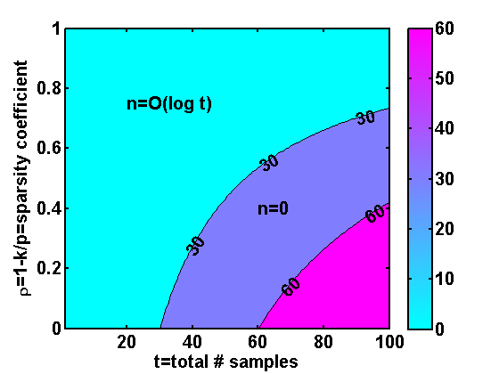
The constant above is an increasing function of the quantity defined in (15). Proposition 4 asserts that for a generous budget ( large) the optimal first stage sampling allocation is . However, when the budget is tight it is better to skip stage 1 (). Figure 3 illustrates the allocation region (for ) as a function of the sparsity coefficient . Note that Prop. 4 is generally true for any two-stage predictor which at the first stage, uses a support recovery method that satisfies the performance bound proposed by Prop. 2 or Prop. 3, and at the second stage uses OLS.

IV Numerical comparisons
We now present experimental results which demonstrate the performance of SPARCS when applied to both synthetic and real world data. Throughout this section we refer to the SPARCS predictors which use SIS or PCS at the first stage as SIS-SPARCS or PCS-SPARCS, respectively.
a) Efficiency of SPARCS screening stage. We illustrate the performance of the SPARCS screening stage (i.e., the first stage of the SPARCS predictor) using SIS or PCS and compare these to LASSO [48, 23].
In the first set of simulations we generated an data matrix with independent rows, each of which is drawn from a -dimensional multivariate normal distribution with mean and block-sparse covariance matrix satisfying (17). The coefficient vector is then generated such that exactly entries of are active. Each active entry of is an independent draw from distribution, and each inactive entry of is zero. Finally, a synthetic response vector is generated by a simple linear model
| (29) |
where is noise vector whose entries are i.i.d. . The importance of a variable is measured by the magnitude of the corresponding entry of .
We implemented LASSO on the above data set using an active set type algorithm - asserted to be one the fastest methods for solving LASSO [36]. In all of our implementations of LASSO, the regularization parameter is tuned to minimize prediction MSE using 2-fold cross validation. To illustrate SPARCS screening stage for a truly high dimensional example, we set and compared SIS and PCS methods with LASSO, for a small number of samples. Figure 4 shows the results of this simulation over an average of independent experiments for each value of . As we see for small number of samples, PCS and SIS methods perform significantly better in selecting the important predictor variables. Moreover, the advantage of the extra pseudo-inverse factor used for variable selection in PCS as compared to SIS is evident in Fig. 4.

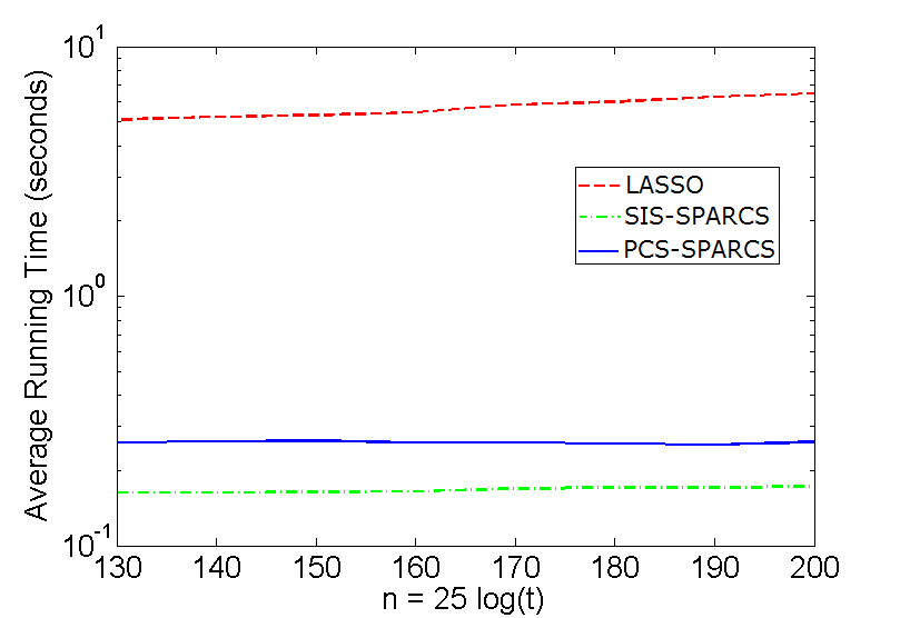
b) Efficiency of the SPARCS predictor. To test the efficiency of the proposed SPARCS predictor, a total of samples are generated using the linear model (29) from which are used for the task of variable selection at the first stage. All samples are then used to compute the OLS estimator restricted to the selected variables. We chose such that . The performance is evaluated by the empirical Root Mean Squared Error
| (30) |
where is the number of simulation trials. Similar to the previous experiment, exactly entries of are active and the predictor variables follow a multivariate normal distribution with mean and block-sparse covariance matrix. Figure 5 shows the result of this simulation for , in terms of performance (left) and running time (right). Each point on these plots is an average of independent experiments. Observe that in this low sample regime, when LASSO or SIS are used instead of PCS in the first stage, the performance suffers. More specifically we observe that the RMSE of the PCS-SPARCS predictor is uniformly lower than the SIS-SPARCS predictor or the two-stage predictor that uses LASSO in the first stage. Table I shows the -values of one-sided paired t-tests testing for differences between the RMSE for PCS-SPARCS and SIS-SPARCS (LASSO) for several different values of . These results show the high statistical significances of these RMSE differences.

| PCS-SPARCS vs. SIS-SPARCS | ||||||||
|---|---|---|---|---|---|---|---|---|
| PCS-SPARCS vs. LASSO |
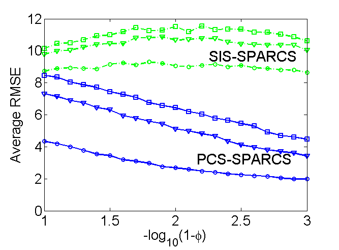
To further indicate the advantage of the PCS-SPARCS predictor compared to the SIS-SPARCS predictor, we performed simulations in which the number of samples used at the first stage, , and the number of samples used at the second stage, , are fixed while the number of variables increases from to . Moreover, exactly entries of the coefficient vector are active. Similar to the previous experiments, samples are generated using the linear model (29). However, in order to generate a data set with high multicollinearity, a scenario that is likely to happen in high dimensional data sets (see [44] and the references therein), here the inactive variables are consecutive samples of an Auto-Regressive (AR) process of the form:
| (31) |
in which ’s are independent draws of . The result of this experiment for is shown in Fig. 6 (left). The average RMSE values are computed using independent experiments. The advantage of using PCS-SPARCS over SIS-SPARCS is evident in Fig. 6 (left). Note that as the number of variables becomes significantly larger than the number of samples , the performance of both of the predictors converge to the performance of a random selection and estimation scheme in which variables are selected at random in the first stage.
Furthermore, to analyze the performance of PCS-SPARCS and SIS-SPARCS for different levels of multicollinearity in the data, we performed similar experiments for as the value of increases from to . Figure 6 (right) shows the result of this simulation. Each point on these plots is the average of independent experiments. It is evident that similar to the previous experiment, the PCS-SPARCS predictor outperforms the SIS-SPARCS predictor. An interesting observation in Fig 6 (right) is that as the multicollinearity coefficient increases the performance of the PCS-SPARCS predictor improves.

c) Estimation of FWER using Monte Carlo simulation. We set and using Monte Carlo simulation, we computed the probability of support recovery error for the PCS method. In order to prevent the coefficients from getting close to zero, the active coefficients were generated via a Bernoulli-Gaussian distribution of the form:
| (32) |
Figure 7 shows the estimated probabilities. Each point of the plot is an average of experiments. As the value of decreases the quantity defined in (15) is bounded away from with high probability and the probability of selection error degrades. As we can see, the FWER decreases at least exponentially with the number of samples. This behavior is consistent with the result in Prop. 3.

d) Application to experimental data. We illustrate the proposed SPARCS predictor on the Predictive Health and Disease data set, which consists of gene expression levels and symptom scores of different subjects. The data was collected during a challenge study for which some subjects become symptomatically ill with the H3N2 flu virus [34]. For each subject, the gene expression levels (for genes) and the clinical symptoms have been recorded at a large number of time points that include pre-inoculation and post-inoculation sample times. Ten different symptom scores were measured. Each symptom score takes an integer value from to , which measures the severity of that symptom at the corresponding time. The goal here is to learn a predictor that can accurately predict the future symptom scores of a subject based on her last measured gene expression levels.
We considered each symptom as a scalar response variable and applied the SPARCS predictor to each symptom separately. In order to do the prediction task, the data used for the SPARCS predictor consists of the samples of the symptom scores for various subjects at specified time points () and their corresponding gene expression levels measured at the previous time points (). The number of predictor variables (genes) selected in the first stage is restricted to . Since, the symptom scores take integer values, the second stage uses multinomial logistic regression instead of the OLS predictor. Maximum likelihood estimation is used for computing the multinomial logistic regression coefficients [1]. The performance is evaluated by leave-one-out cross validation. To do this, the data from all except one subject are used as training samples and the data from the remaining subject are used as the test samples. The final RMSE is then computed as the average over the different leave-one-out cross validation trials. In each of the experiments out of the subjects of the training set, are used in first stage and all of the subjects are used in the second stage. It is notable that PCS-SPARCS performs better in predicting the symptom scores for of the symptoms whereas SIS-SPARCS and LASSO perform better in predicting the symptom scores for symptoms and symptom, respectively.
| Symptom | RMSE: LASSO | RMSE: SIS-SPARCS | RMSE: PCS-SPARCS |
|---|---|---|---|
| Runny Nose | 0.7182 | 0.6896 | 0.6559 |
| Stuffy Nose | 0.9242 | 0.7787 | 0.8383 |
| Sneezing | 0.7453 | 0.6201 | 0.6037 |
| Sore Throat | 0.8235 | 0.7202 | 0.5965 |
| Earache | 0.2896 | 0.3226 | 0.3226 |
| Malaise | 1.0009 | 0.7566 | 0.9125 |
| Cough | 0.5879 | 0.7505 | 0.5564 |
| Shortness of Breath | 0.4361 | 0.5206 | 0.4022 |
| Headache | 0.7896 | 0.7500 | 0.6671 |
| Myalgia | 0.6372 | 0.5539 | 0.4610 |
| Average for all symptoms | 0.6953 | 0.6463 | 0.6016 |
V Conclusion
We proposed an online procedure for budget-limited predictor design in high dimensions dubbed two-stage Sampling, Prediction and Adaptive Regression via Correlation Screening (SPARCS). SPARCS is specifically useful in cases where and the high cost of assaying all predictor variables justifies a two-stage design: high throughput variable selection followed by predictor construction using fewer selected variables. We established high dimensional false discovery rates, support recovery guarantees, and optimal stage-wise sample allocation rule associated with the SPARCS online procedure. Simulation and experimental results showed advantages of SPARCS as compared to LASSO. Our future work includes using SPARCS in a multi-stage framework. We believe that multi-stage SPARCS can further improve the performance of the algorithm while benefiting from high computational efficiency.
VI Appendix
This section contains three subsections. Section VI-A provides the proof of Lemma 2. Section VI-B introduces the necessary notations for the proofs of the remaining propositions. Section VI-C gives the proofs for the propositions presented in Sec. III.
VI-A Lemma 2 and U-score representations
Below we present the proof of Lemma 2 which states that both SIS and PCS methods for discovering the support are equivalent to discovering the non-zero entries of some vector with representation (18) by thresholding at a specified threshold.
Proof of Lemma 2: Using the U-score representation of the correlation matrices, there exist a matrix with unit norm columns, and a unit norm vector such that [30, 31]:
| (33) |
Representation (33) immediately shows that SIS is equivalent to discovering non-zero entries of a vector with representation (18). Moreover, we have
| (34) |
and:
| (35) |
where denotes the diagonal matrix obtained by zeroing out the off-diagonals of square matrix . We refer the interested reader to [31, 2] for more information about the calculations of U-scores. Using representations (34) and (35), one can write:
| (36) | |||||
Defining , we have:
| (37) |
where
| (38) |
Note that the columns of the matrix lie on since the diagonal entries of the matrix are equal to one. Therefore, a U-score representation of the generalized OLS solution can be obtained as:
| (39) | |||||
Without loss of generality we can consider the case where . Given the concentration property (14), asymptotically we have , with probability 1. Moreover Assumption 3 yields the asymptotic relationship . Therefore, finding the largest entries of is equivalent to finding the largest entries of as the ordering of the entries will asymptotically stay unchanged. This motivates screening for non-zero entries of the vector instead of the entries of . In particular, for a threshold , we can undertake variable selection by discovering the entries of the vector in (38) that have absolute values at least . This implies that discovering the support via PCS is equivalent to discovering the non-zero entries of in (38) which admits the representation (18). The proof for SIS follows similarly. ∎
VI-B Notations and preliminaries
The following additional notations are necessary for the remaining propositions and the proofs presented in this section.
For arbitrary joint densities defined on the Cartesian product , define
| (40) |
The quantity is key in determining the expected number of discoveries in screening the entries of the vector in (18).
In the following propositions, represents an upper bound on the number of entries in any row or column of covariance matrix or cross-covariance vector that do not converge to zero as . We define , the average dependency coefficient, as:
| (41) |
with
| (42) |
in which is defined as the set complement of indices of the -nearest neighbors of (i.e. the complement of indices of the entries with largest magnitude in the -th row of ). Finally, the function of the joint density is defined as:
| (43) |
The function plays a key role in the asymptotic expression for the mean number of discoveries. Note that when observations are independent, by symmetry, the marginal distributions of -scores are exchangeable, i.e.,
| (44) |
for any permutation matrix . Therefore, the joint distribution must yield exchangeable marginals.
We now present two examples for which has a closed form expression.
Example 1. If the joint distribution is uniform over the product ,
| (45) | |||||
Example 2. Consider the case where the joint distribution is separable of the form
| (46) |
i.e., and are independent. Let the marginals be von Mises-Fisher distributions over the sphere
| (47) |
in which and are the location parameter and the concentration parameter, respectively, and is a normalization constant, calculated as:
| (48) |
where is the modified Bessel function of the first kind of order . can be computed up to the desired precision using the expansion:
| (49) |
in which is the gamma function.
Due to exchangeability of , the only two feasible choices for are and , where . Hence the joint distribution can be written as:
| (50) | |||||
Assuming and , where , we obtain:
| (51) | |||||
This yields:
| (52) | |||||
Therefore, using (48) and (49), can be computed up to the desired precision.
Further properties as well as intuitive interpretations of have also been considered in [30].
VI-C Proofs of propositions
We first prove the following more general version of Prop. 1. This generalization can be useful in obtaining an approximate false discovery rates for SPARCS screening stage in cases where the underlying distribution of data is known.
Proposition 5
Consider the linear model (13) for which Assumption 1 is satisfied. Let and be and random matrices with unit norm columns. Let be a sequence of threshold values in such that as and . Throughout this proposition denotes the number of entries of the vector whose magnitude is at least . We have:
| (53) | |||||
where and .
Assume also that and
that the limit of average dependency coefficient satisfies . Then:
| (54) |
with
| (55) |
Proof of Prop. 5: Let denote the degree of vertex in part of the graph . We have:
| (56) |
The following representation for holds:
| (57) |
where is the union of two anti-polar caps in of radius centered at and . The following inequality will be helpful:
| (58) |
| (59) |
where , and is a simplified notation for . Also for we have:
| (60) |
where
is a bound on the conditional joint densities of the form .
Application of the mean value theorem to the integral
representation (58) yields:
| (61) |
where and is a bound on the norm of the gradient:
| (62) |
Using (61) and the relation we conclude:
| (63) |
Summing up over we conclude:
| (64) |
where .
This concludes (53).
To prove the second part of the theorem, we use Chen-Stein method
[4]. Define the index set
, where is the set of indices of the -nearest neighbors of . Note that
. Assume is a Poisson random variable with
. Using
theorem 1 of [4], we have:
| (65) |
where:
| (66) | |||
| (67) |
and
| (68) |
where . Using the bound (59), is of order . Therefore:
| (69) |
Since , applying (60) to each term of the summation (67) gives:
| (70) |
Finally, to bound we have:
| (71) |
Therefore using bound (64) we obtain:
| (72) | |||||
Combining this with the bounds on and , completes the proof of (54). ∎
In order to obtain stronger bounds, we prove the Prop. 1 under the weakly block-sparse assumption (17). However the proof for the general case where Assumption 3 is satisfied follow similarly.
Lemma 3
Proof of Lemma 3 : We have:
| (78) |
By block sparsity of can be partitioned as:
| (79) |
where are the U-scores corresponding to the dependent block of and are the remaining U-scores.
Using the law of large numbers for a sequence of correlated variables (see, e.g., Example 11.18 in [46]) since the off-diagonal entries of that are not in the dependent block converge to as grows, we have
| (80) |
Since the entries of are bounded by one, we have:
| (81) |
where is an matrix whose entries are . Hence:
| (82) |
Hence, as :
| (83) |
Thus:
| (84) |
Now we prove relations (74)-(77). Define the partition of the index set , where is asymptotically uncorrelated of . We have:
| (85) |
and
| (86) |
But, for and for . Moreover, we have , where . Therefore,:
| (87) |
Moreover, since , . This concludes:
| (88) |
and
| (89) |
∎
Proof of Lemma 1: By block sparsity of can be partitioned as:
| (90) |
where are the U-scores corresponding to the dependent block of and are the remaining U-scores. Using relations (80) and (81) we have:
| (91) |
Noting that the result follows.∎
The following lemma will be useful in the proof of proof of Prop. 2.
Lemma 4
Assume and are jointly elliptically contoured distributed random variables from which joint observations are available. Further assume that the matrix of these observations has an elliptically contoured distribution of the form given in Assumption 1. Let and . Also let and , be the corresponding sample correlation coefficients. Assume that . Then, there exists and such that:
| (92) |
for all .
We use the following lemma to prove Lemma 4.
Lemma 5
Let and be two independent uniformly distributed random vectors on . For any fixed , there exists such that:
| (93) |
Proof of Lemma 5: Without loss of generality assume . We have
| (94) |
in which is the first entry of the vector . Using the formula for the area of spherical cap [40] we obtain
| (95) |
where , and
| (96) |
is the regularized incomplete beta function. Note that:
| (97) |
Therefore by letting we obtain
| (98) |
∎
Proof of Lemma 4: Let . Assume follows an elliptically contoured density function of the form . Without loss of generality assume . Using a Cholesky factorization we can represent and as linear combination of uncorrelated random variables and which follow a spherically contoured distribution:
| (99) |
where
| (100) | |||
| (101) | |||
| (102) |
and
| (103) |
Let . Since follows a spherically contoured distribution, it has a stochastic representation of the form , where has a marginal density , in which is a normalizing constant. Moreover is independent of and the distribution of does not depend on the function (see, e.g., Chapter 2 in [2] for more details about such stochastic representation). Now let and denote the U-scores corresponding to independent samples of and , respectively. Then under Assumption 1, as these U-scores are invariant to translation and scale on the samples of , the joint distribution of the U-scores does not depend on and without loss of generality the samples can be assumed to be i.i.d. Gaussian [3]. Similarly, let and denote the U-scores corresponding to and , respectively. Using (99) we have the following relations:
| (104) | |||||
Hence
| (105) |
and
| (106) | |||||
Now let . We have:
| (107) |
Since
| (108) |
and, by using triangle inequality, we have
| (109) |
Note that by assumption . Now by Lemma 5 we get
| (110) |
with
| (111) | |||||
where the last inequality is obtained via equations (100)-(103). Letting and we have
| (112) |
for . ∎
Proof of Proposition 2: Since increases as the size of the recovered set increases, it suffices to prove the proposition for . Define an auxiliary random variable such that . Note that by Assumption 2 . For we have:
| (113) | |||
Now since Assumptions 1 and 2 are satisfied, by Lemma 4 there exist constants and a constant such that
| (114) |
in which . Hence by letting and we have:
| (115) |
and
| (116) |
which completes the proof. ∎
Proof of Proposition 3: We only provide a proof sketch here. By Assumption 3 we have
| (117) |
Therefore:
| (118) |
Since columns of have unit norm we obtain:
| (119) |
and
| (120) |
This yields
| (121) |
which implies
| (122) | |||||
where, by the concentration assumption, with high probability the term decays to 0 exponentially fast. Therefore screening the entries of or is asymptotically equivalent to selecting the support via thresholding the entries of , i.e., the sample correlation coefficients. Therefore the proof follows from Prop. 2. ∎
Proof of Proposition 4: First we consider a two-stage predictor similar to the one introduced in Sec. II with the difference that the samples which are used in stage are not used in stage . Therefore, there are and samples used in the first and the second stages, respectively. We represent this two-stage predictor by . Similarly, denotes the SPARCS algorithm which uses samples at the first stage and all of the samples at the second stage. The asymptotic results for the two-stage predictor will be shown to hold as well for the two-stage predictor.
Using inequalities of the form (113) and the union bound, it is straightforward to see that for any subset of elements of , the probability that is the outcome of variable selection via SPARCS, is bounded above by , in which is a constant that is bounded above by . The expected MSE of the algorithm can be written as:
| (123) |
where is the set of all -subsets of , is the probability that the outcome of variable selection via SPARCS is the subset , and is the MSE of OLS stage when the indices of the selected variables are the elements of . Therefore the expected MSE is upper bounded as below:
| (124) |
where is a constant which is upper bounded by . It can be shown that if there is at least one wrong variable selected (), the OLS estimator is biased and the expected MSE converges to a positive constant as . When all the variables are selected correctly (subset ), MSE goes to zero with rate . Hence:
| (125) |
where and are constants that do not depend on or but depend on the quantities and . Note that . This quantity is an increasing function .
On the other hand since at most variables could be used in OLS stage, the expected MSE is lower bounded:
| (126) |
It can be seen that the minimum of (125) as a function of , subject to the constraint (1), happens for if with (therefore, similar to , is increasing in ); otherwise it happens for 0. If , the minimum value attained by the upper bound (125) is which is as low as the lower bound (126). This shows that for large , the optimal number of samples that should be assigned to the SPARCS stage of the predictor is . As , since , the MSE of the predictor proposed in Sec. II converges to the MSE of the predictor. Therefore, as , becomes optimal for the predictor as well. ∎
References
- [1] A. Albert and J. Anderson, “On the existence of maximum likelihood estimates in logistic regression models,” Biometrika, vol. 71, no. 1, pp. 1–10, 1984.
- [2] T. W. Anderson, An introduction to multivariate statistical analysis, Wiley, 2003.
- [3] T. W. Anderson, “Nonnormal multivariate distributions: Inference based on elliptically contoured distributions,” Technical report, DTIC Document, 1992.
- [4] R. Arratia, L. Goldstein, and L. Gordon, “Poisson approximation and the chen-stein method,” Statistical Science, vol. 5, no. 4, pp. 403–424, 1990.
- [5] J.-Y. Audibert, R. Munos, and C. Szepesvári, “Tuning bandit algorithms in stochastic environments,” in Algorithmic Learning Theory, pp. 150–165. Springer, 2007.
- [6] R. G. Baraniuk, V. Cevher, M. F. Duarte, and C. Hegde, “Model-based compressive sensing,” Information Theory, IEEE Transactions on, vol. 56, no. 4, pp. 1982–2001, 2010.
- [7] R. E. Bechhofer, J. Kiefer, and M. Sobel, Sequential identification and ranking procedures: with special reference to Koopman-Darmois populations, volume 3, University of Chicago Press Chicago, 1968.
- [8] M. Biguesh and A. B. Gershman, “Training-based mimo channel estimation: a study of estimator tradeoffs and optimal training signals,” Signal Processing, IEEE Transactions on, vol. 54, no. 3, pp. 884–893, 2006.
- [9] P. Bühlmann, “Boosting for high-dimensional linear models,” The Annals of Statistics, vol. 34, no. 2, pp. 559–583, 2006.
- [10] P. Bühlmann and S. Van De Geer, Statistics for High-Dimensional Data: Methods, Theory and Applications, Springer, 2011.
- [11] E. Candés, J. Romberg, and T. Tao, “Stable signal recovery from incomplete and inaccurate measurements,” Comm. Pure Appl. Math., vol. 59, pp. 1207–1223, 2005.
- [12] E. Candes and J. Romberg, “Sparsity and incoherence in compressive sampling,” Inverse problems, vol. 23, no. 3, pp. 969, 2007.
- [13] L. Carin, D. Liu, and B. Guo, “Coherence, compressive sensing, and random sensor arrays,” Antennas and Propagation Magazine, IEEE, vol. 53, no. 4, pp. 28–39, 2011.
- [14] C. Ding, X. He, H. Zha, and H. D. Simon, “Adaptive dimension reduction for clustering high dimensional data,” in Data Mining, 2002. ICDM 2003. Proceedings. 2002 IEEE International Conference on, pp. 147–154. IEEE, 2002.
- [15] D. L. Donoho, “Compressed sensing,” Information Theory, IEEE Transactions on, vol. 52, no. 4, pp. 1289–1306, 2006.
- [16] B. Efron, T. Hastie, I. Johnstone, and R. Tibshirani, “Least angle regression,” The Annals of statistics, vol. 32, no. 2, pp. 407–499, 2004.
- [17] J. Fan and J. Lv, “Sure independence screening for ultrahigh dimensional feature space,” Journal of the Royal Statistical Society: Series B (Statistical Methodology), vol. 70, no. 5, pp. 849–911, 2008.
- [18] J. Fan, R. Song, et al., “Sure independence screening in generalized linear models with np-dimensionality,” The Annals of Statistics, vol. 38, no. 6, pp. 3567–3604, 2010.
- [19] M. A. Figueiredo, R. D. Nowak, and S. J. Wright, “Gradient projection for sparse reconstruction: Application to compressed sensing and other inverse problems,” Selected Topics in Signal Processing, IEEE Journal of, vol. 1, no. 4, pp. 586–597, 2007.
- [20] G. Forman, “An extensive empirical study of feature selection metrics for text classification,” The Journal of machine learning research, vol. 3, pp. 1289–1305, 2003.
- [21] J. Friedman, T. Hastie, and R. Tibshirani, The elements of statistical learning, volume 1, Springer Series in Statistics, 2001.
- [22] C. Genovese, J. Jin, and L. Wasserman, “Revisiting marginal regression,”, 2009.
- [23] C. R. Genovese, J. Jin, L. Wasserman, and Z. Yao, “A comparison of the lasso and marginal regression,” The Journal of Machine Learning Research, vol. 98888, pp. 2107–2143, 2012.
- [24] T. R. Golub, D. K. Slonim, P. Tamayo, C. Huard, M. Gaasenbeek, J. P. Mesirov, H. Coller, M. L. Loh, J. R. Downing, M. A. Caligiuri, et al., “Molecular classification of cancer: class discovery and class prediction by gene expression monitoring,” science, vol. 286, no. 5439, pp. 531–537, 1999.
- [25] S. S. Gupta and S. Panchapakesan, “Sequential ranking and selection procedures,” Handbook of sequential analysis, pp. 363–380, 1991.
- [26] I. Guyon and A. Elisseeff, “An introduction to variable and feature selection,” The Journal of Machine Learning Research, vol. 3, pp. 1157–1182, 2003.
- [27] B. Hassibi and B. Hochwald, “How much training is needed in multiple-antenna wireless links?,” Information Theory, IEEE Transactions on, vol. 49, no. 4, pp. 951–963, April 2003.
- [28] J. Haupt, R. M. Castro, and R. Nowak, “Distilled sensing: Adaptive sampling for sparse detection and estimation,” Information Theory, IEEE Transactions on, vol. 57, no. 9, pp. 6222–6235, 2011.
- [29] J. D. Haupt, R. G. Baraniuk, R. M. Castro, and R. D. Nowak, “Compressive distilled sensing: Sparse recovery using adaptivity in compressive measurements,” in Signals, Systems and Computers, 2009 Conference Record of the Forty-Third Asilomar Conference on, pp. 1551–1555. IEEE, 2009.
- [30] A. Hero and B. Rajaratnam, “Large-scale correlation screening,” Journal of the American Statistical Association, vol. 106, no. 496, pp. 1540–1552, 2011.
- [31] A. Hero and B. Rajaratnam, “Hub discovery in partial correlation graphs,” Information Theory, IEEE Transactions on, vol. 58, no. 9, pp. 6064–6078, 2012.
- [32] T. Hesterberg, N. H. Choi, L. Meier, C. Fraley, et al., “Least angle and ℓ1 penalized regression: A review,” Statistics Surveys, vol. 2, pp. 61–93, 2008.
- [33] J. C. Huang and N. Jojic, “Variable selection through correlation sifting,” in Research in Computational Molecular Biology, pp. 106–123. Springer, 2011.
- [34] Y. Huang, A. K. Zaas, A. Rao, N. Dobigeon, P. J. Woolf, T. Veldman, N. C. Øien, M. T. McClain, J. B. Varkey, B. Nicholson, et al., “Temporal dynamics of host molecular responses differentiate symptomatic and asymptomatic influenza a infection,” PLoS genetics, vol. 7, no. 8, pp. e1002234, 2011.
- [35] J. A. Khan, S. Van Aelst, and R. H. Zamar, “Robust linear model selection based on least angle regression,” Journal of the American Statistical Association, vol. 102, no. 480, pp. 1289–1299, 2007.
- [36] J. Kim and H. Park, “Fast active-set-type algorithms for l1-regularized linear regression,” Proc. AISTAT, pp. 397–404, 2010.
- [37] S.-J. Kim, K. Koh, M. Lustig, S. Boyd, and D. Gorinevsky, “An interior-point method for large-scale l 1-regularized least squares,” Selected Topics in Signal Processing, IEEE Journal of, vol. 1, no. 4, pp. 606–617, 2007.
- [38] K. Koh, S.-J. Kim, and S. P. Boyd, “An interior-point method for large-scale l1-regularized logistic regression.,” Journal of Machine learning research, vol. 8, no. 8, pp. 1519–1555, 2007.
- [39] V. Koltchinskii and K. Lounici, “Concentration inequalities and moment bounds for sample covariance operators,” arXiv preprint arXiv:1405.2468, 2014.
- [40] S. Li, “Concise formulas for the area and volume of a hyperspherical cap,” Asian Journal of Mathematics and Statistics, vol. 4, no. 1, pp. 66–70, 2011.
- [41] G. Obozinski, M. J. Wainwright, M. I. Jordan, et al., “Support union recovery in high-dimensional multivariate regression,” The Annals of Statistics, vol. 39, no. 1, pp. 1–47, 2011.
- [42] D. Paul, E. Bair, T. Hastie, and R. Tibshirani, “” preconditioning” for feature selection and regression in high-dimensional problems,” The Annals of Statistics, pp. 1595–1618, 2008.
- [43] A. Quattoni, X. Carreras, M. Collins, and T. Darrell, “An efficient projection for l 1,∞ regularization,” in Proceedings of the 26th Annual International Conference on Machine Learning, pp. 857–864. ACM, 2009.
- [44] B. Rajaratnam, S. Roberts, D. Sparks, and O. Dalal, “The deterministic bayesian lasso,” arXiv preprint arXiv:1401.2480, 2014.
- [45] Y. Rong, Practical environmental statistics and data analysis, ILM Publications, 2011.
- [46] T. A. Severini, Elements of distribution theory, volume 17, Cambridge University Press, 2005.
- [47] C. Suh, S. C. Sieg, M. J. Heying, J. H. Oliver, W. F. Maier, and K. Rajan, “Visualization of high-dimensional combinatorial catalysis data,” Journal of combinatorial chemistry, vol. 11, no. 3, pp. 385–392, 2009.
- [48] R. Tibshirani, “Regression shrinkage and selection via the lasso,” Journal of the Royal Statistical Society. Series B (Methodological), pp. 267–288, 1996.
- [49] J. A. Tropp and A. C. Gilbert, “Signal recovery from random measurements via orthogonal matching pursuit,” Information Theory, IEEE Transactions on, vol. 53, no. 12, pp. 4655–4666, 2007.
- [50] M. J. Wainwright, “Sharp thresholds for high-dimensional and noisy sparsity recovery using-constrained quadratic programming (lasso),” Information Theory, IEEE Transactions on, vol. 55, no. 5, pp. 2183–2202, 2009.
- [51] A. Wald et al., “Sequential tests of statistical hypotheses,” Annals of Mathematical Statistics, vol. 16, no. 2, pp. 117–186, 1945.
- [52] F. L. Wauthier, N. Jojic, and M. Jordan, “A comparative framework for preconditioned lasso algorithms,” in Advances in Neural Information Processing Systems, pp. 1061–1069, 2013.
- [53] D. Wei and A. O. Hero, “Multistage adaptive estimation of sparse signals,” Selected Topics in Signal Processing, IEEE Journal of, vol. 7, no. 5, pp. 783–796, 2013.
- [54] D. Wei and A. O. Hero, “Performance guarantees for adaptive estimation of sparse signals,” arXiv preprint arXiv:1311.6360, 2013.
- [55] Z. Wen, W. Yin, D. Goldfarb, and Y. Zhang, “A fast algorithm for sparse reconstruction based on shrinkage, subspace optimization, and continuation,” SIAM Journal on Scientific Computing, vol. 32, no. 4, pp. 1832–1857, 2010.
- [56] Z. Wen, W. Yin, H. Zhang, and D. Goldfarb, “On the convergence of an active-set method for ℓ1 minimization,” Optimization Methods and Software, vol. 27, no. 6, pp. 1127–1146, 2012.
- [57] M. Yuan and Y. Lin, “Model selection and estimation in regression with grouped variables,” Journal of the Royal Statistical Society: Series B (Statistical Methodology), vol. 68, no. 1, pp. 49–67, 2005.
![[Uncaptioned image]](1502.06189v2/FirouziNov2013.png) |
Hamed Firouzi received the B.Sc. degrees in Electrical Engineering and Pure Mathematics from Sharif University of Technology, Tehran, Iran, in 2009, and the M.Sc. degrees in Financial Engineering and Applied Mathematics, from the University of Michigan, Ann Arbor, MI, USA, in 2014. He received the PhD degree in Electrical Engineering from the University of Michigan, Ann Arbor, MI, USA, in 2015. He is currently a quantitative modeler at the Goldman Sachs Group, Inc. His research interests include predictive modeling, machine learning, pattern recognition, data science, statistical signal processing, and financial modeling. |
![[Uncaptioned image]](1502.06189v2/HeroJan2010.png) |
Alfred O. Hero III is the John H. Holland Distinguished University Professor of Electrical Engineering and Computer Science and the R. Jamison and Betty Williams Professor of Engineering at the University of Michigan, Ann Arbor. He is also the Co-Director of the University’s Michigan Institute for Data Science (MIDAS). His primary appointment is in the Department of Electrical Engineering and Computer Science and he also has appointments, by courtesy, in the Department of Biomedical Engineering and the Department of Statistics. He received the B.S. (summa cum laude) from Boston University (1980) and the Ph.D from Princeton University (1984), both in Electrical Engineering. He is a Fellow of the Institute of Electrical and Electronics Engineers (IEEE). He has served as President of the IEEE Signal Processing Society and as a member of the IEEE Board of Directors. He has received numerous awards for his scientific research and service to the profession including the IEEE Signal Processing Society Technical Achievement Award in 2013 and the 2015 Society Award, which is the highest career award bestowed by the IEEE Signal Processing Society. Alfred Hero’s recent research interests are in high dimensional spatio-temporal data, multi-modal data integration, statistical signal processing, and machine learning. Of particular interest are applications to social networks, network security and forensics, computer vision, and personalized health. |
![[Uncaptioned image]](1502.06189v2/Rajaratnam.png) |
Bala Rajaratnam received the B.Sc.(Hons)/M.Sc. degrees from the University of the Witwatersrand, Johannesburg, South Africa, in 1999 and the M.S./Ph.D. degrees from Cornell University, Ithaca, NY, USA, in 2006. He is a faculty member at the Department of Statistics at Stanford University, Stanford and the University of California Davis, CA, USA. He is also a visiting professor at the University of Sydney, Australia. His research interests include graphical models, machine learning, data science, high-dimensional inference, signal processing, spatio–temporal and environmental modeling, financial engineering, positivity and the mathematics of networks. Mr. Rajaratnam is the recipient of several awards and recognitions including two federal CAREER awards, the National Science Foundation (NSF) CAREER Award, and the Defense Advanced Research Projects Agency (DARPA) Young Faculty Award. |