Surface morphology coarsening in a nonlocal system
Abstract
Direct comparison is made of the steady-sates and coarsening dynamics in a local system and its nonlocal generalization. The example system is the surface of a solid film in a strong electric field; the morphological evolution of the surface is described, in the long-wavelength approximation, by the amplitude PDE for the film height function. It is shown that the amplitude of the steady-state and the coarsening rate of the surface structure are very sensitive to the radius of the long-range interaction, and that both quantities increase as the radius decreases.
pacs
68.55.J,81.15.Aa,81.16.DnNonlocal pattern forming systems with long-range interactions, described by a nonlinear partial integro-differential equations, are ubiquitous in science and engineering. One can mention Rayleigh-Benard convection [1], magnetoconvection [2], surfactant-mediated interfacial flows [3], instabilities in plasma [4, 5], flow of a film down an inclined plane in the electric field [6, 7], vibrated layers of a granular material or viscoelastic fluid [8], evaporation of liquid films [9], and reaction-diffusion systems [10, 11].
In materials science, evolution of phases of a binary alloy is described by a Cahn-Hilliard (CH) equation for an order parameter; the impacts of long-range interactions on coarsening of the order parameter have been studied [12, 13, 14, 15]. Also, guided by their analysis of Asaro-Tiller-Grinfeld instability in heteroepitaxial solid films, Kassner and Misbah [16] proposed the “generic” nonlocal amplitude equation, derived in the long-wave limit:
| (1) |
where is the film height above the substrate, are parameters, and
| (2) | |||||
is the Hilbert transform on the real line (p.v. stands for Cauchy principal value). Eq. (1), being relevant to systems where the linear dispersion relation is quadratic, is complementary to the Kuramoto-Sivashinsky equation. Although these authors computed Eq. (1) and determined that it describes a perpetual coarsening, the account of their investigation is very brief (one figure displaying a qualitative behavior); in particular, they did not investigate how the non-local terms affect the coarsening exponents. Nor were the effects of the finite radius of the long-range interactions studied.

In this short note, we directly compare coarsening in the local and nonlocal systems described by a long-wave evolution equations for the film height. These equations stem from the consideration of the surface electromigration [18, 19, 20, 21, 22], an intrinsically nonlocal effect. Assuming the constant electric field parallel to the substrate and using the local aproximation for the field on the film surface, (where is the surface orientation angle), the local, conserved evolution equation reads [23]:
| (3) | |||||
where is the “Mullins number” characterizing the strength of the natural surface diffusion, is the electric field strength parameter, and is the derivative of the (anisotropic) adatom’s diffusional mobility at the planar surface . Under (dimensionless) Eq. (3) a random, short-wavelength initial deformation of the infinite planar surface perpetually coarsens - the size of the structures increases as a power law in time [19, 23, 24].

Guided by Ref. [16], the nonlocal generalization of this equation is:
| (4) | |||||
where
| (5) |
is the interaction radius. We compute Hilbert transform using fast method from Ref. [17]. The reason we focus on Eq. (4), rather than
| (6) | |||||
is because the latter equation describes the unlimited slope growth, and thus it does not allow to quantify the long-time effects of the nonlocal terms. The unlimited slope growth is inconsistent with the fully nonlocal computations of the morphology evolution using the moving boundary problem [19] (where the electric field is computed in the bulk of the film using the Laplace equation for the electrical potential).
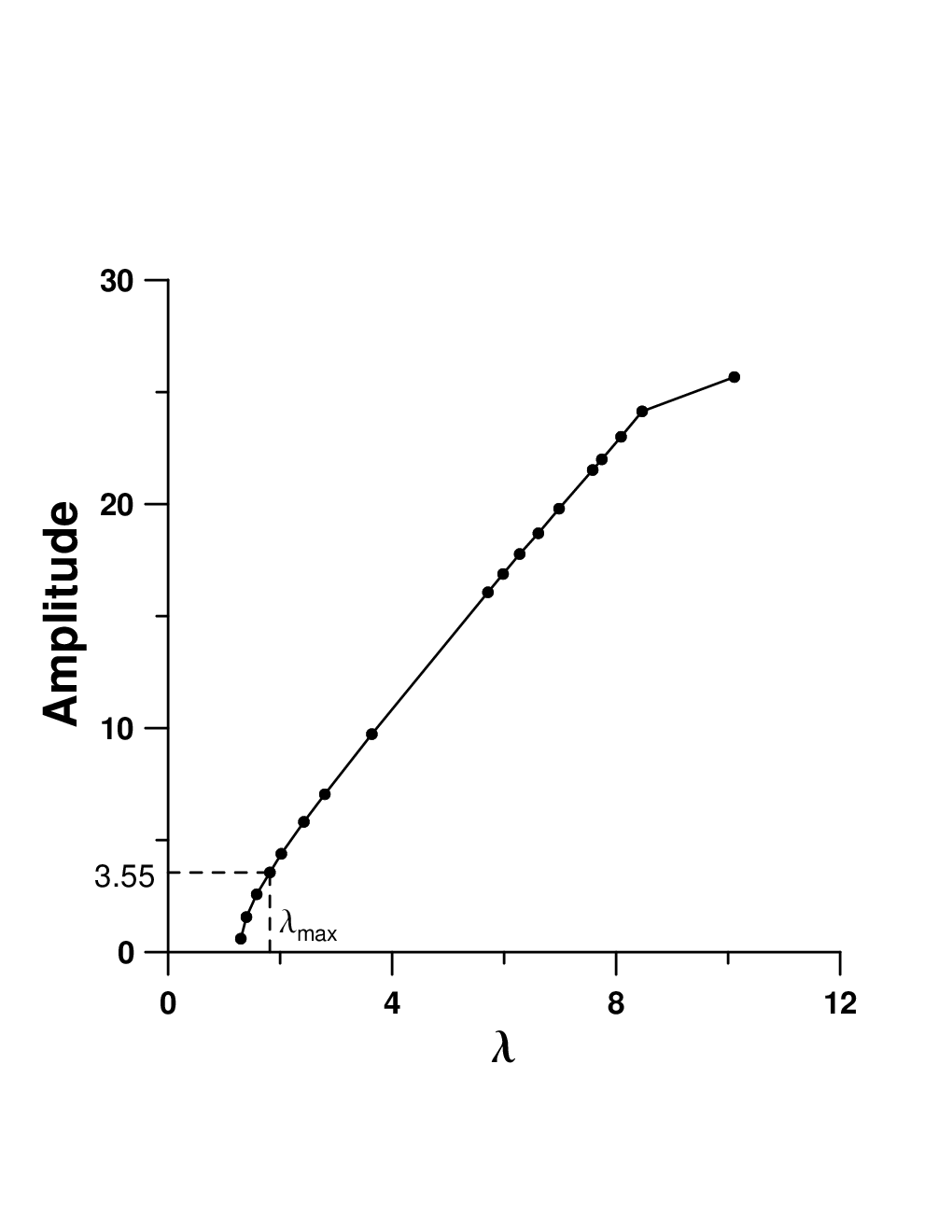
Fig. 1 shows the steady-state profiles from the initial condition , where is the most dangerous wavenumber from the linear stability analysis of Eqs. (3) and (4), and is the corresponding wavelength. The boundary conditions at are periodic. in Fig. 1 is represented by one half of the number of the grid points, , over which the integral in Eq. (5) is computed (that is, to compute the transform at , the points are used). (Eq. 2) corresponds to all points involved, . It can be seen that when the steady-state amplitude is only slightly smaller than the one from the local Eq. (3), and the deviation from the local equation increases as the radius decreases. To re-affirm these results, in Fig. 2 we plot the steady-state amplitude and maximum slope vs. ; both quantities decrease fast initially and level off already at . And, from the monotonicity of the graph of the amplitude of the steady-state vs. the wavelength (Fig. 3) one concludes that coarsening is uninterrupted in a nonlocal system [25, 26].
Next, we performed computations of coarsening using Eqs. (3) and (4). All such computations are done on the domain with the periodic boundary conditions. The results are averaged over five runs with a different random initial condition, and numerical convergence is checked on large grids. Here (Eq. 2) corresponds to . In Figures 4(a,b) is the horizontal scale of the surface structure, e.g. the mean size of a hill at its base. One can see that coarsening is very slow for large (or ) and speeds up when decreases, with the rate approaching one from the local equation as . The major speed-up occurs in a quenching fashion when decreases from 8 to 5, and from there the speed-up is gradual. Also the coarsening rate is very weakly sensitive to for (Fig. 4(b)).
The coarsening exponent in the local model, Eq. (3), initially is of the order reported in Ref. [18] for a similar local model (0.4 vs. 0.3), then it decreases sharply for the rest of the evolution. In the nonlocal model, as increases, the initial regime is confined to the progressively shorter time intervals, and then coarsening becomes logarithmically slow. The initial power law coarsening is matched to the logarithmic law by a power law with a smaller exponent, as shown in the inset of Fig. 4(a).


References
- [1] Christen T. and Elmer F.J., Phys. Lett. A, 150 (1990) 166.
- [2] Dawes J.H.P. and Penington C.J., Geophys. and Astrophys. Fluid Dyn., 106 (2012) 372.
- [3] Bassom A.P., Blyth M.G. and Papageorgiou D.T., Phys. Fluids, 22 (2010) 102102.
- [4] Balmforth N.J. and Kerswell R.R., J. Plasma Phys., 68 (2002) 87.
- [5] Brambilla M. and Bilato R., Nucl. Fusion, 49 (2009) 085004.
- [6] González A. and Castellanos A., Phys. Rev. E, 53 (1996) 3573.
- [7] Duan J.Q. and Ervin V.J., J. Diff. Eq., 143 (1998) 243.
- [8] Dawes J.H.P. and Lilley S., SIAM J. Appl. Dyn. Syst., 9 (2010) 238.
- [9] Sultan E., Boudaoud A. and Ben Amar M., J. Eng. Math., 50 (2004) 209.
- [10] Apreutesei N., Bessonov N. and Volpert V., Discr. Cont. Dyn. Syst. B, 13 (2010) 537.
- [11] Sander E. and Tatum R., Electronic J. Diff. Eq., 160 (2012) 1.
- [12] Fife P., Trends in Nonlinear Analysis, (2003) 153.
- [13] Rubinstein J. and Sternberg P., IMA J. Appl. Math, 48 (1992) 249.
- [14] Guan Z., Lowengrub J.S., Wang C. and Wise S.M., J. Comput. Phys., 277 (2014) 48.
- [15] Slepcev D., SIAM J. Math. Anal., 40 (2008) 1029.
- [16] Kassner K. and Misbah C., Phys. Rev. E, 66 (2002) 026102.
- [17] Bilato R., Maj O. and Brambilla M, Adv. Comput. Math., 40 (2014) 1159.
- [18] Krug J. and Dobbs H.T., Phys. Rev. Lett., 73 (1994) 1947.
- [19] Schimschak M. and Krug J., Phys. Rev. Lett., 78 (1997) 278.
- [20] Mahadevan M. and Bradley R.M., Phys. Rev. B, 59 (1999) 11037.
- [21] Dufay M., Debierre J.-M. and Frisch T., Phys. Rev. B, 75 (2007) 045413.
- [22] Barakat F., Martens K. and Pierre-Louis O., Phys. Rev. Lett., 109 (2012) 056101.
- [23] Khenner M., C. R. Physique, 14 (2013) 607.
- [24] Khenner M. and Bandegi M., to appear in Math. Model. Nat. Phenom. (preprint available: http://arxiv.org/abs/1412.4642)
- [25] Politi P. and Misbah C., Phys. Rev. Lett., 92 (2004) 090601.
- [26] Politi P. and Misbah C., Phys. Rev. E, 73 (2006) 036133.