(Un)conditional consensus emergence under feedback controls
Abstract
We study the problem of consensus emergence in multi-agent systems via external feedback controllers. We consider a set of agents interacting with dynamics given by a Cucker-Smale type of model, and study its consensus stabilization by means of centralized and decentralized control configurations. We present a characterization of consensus emergence for systems with different feedback structures, such as leader-based configurations, perturbed information feedback, and feedback computed upon spatially confined information. We characterize consensus emergence for this latter design as a parameter-dependent transition regime between self-regulation and centralized feedback stabilization. Numerical experiments illustrate the different features of the proposed designs.
Mattia Bongini and Massimo Fornasier
Technische Universität München, Fakultät Mathematik
Boltzmannstraße 3, D-85748 Garching, Germany
Dante Kalise
Radon Institute for Computational and Applied Mathematics, Austrian Academy of Sciences
Altenbergerstraße 69, A-4040 Linz, Austria
1 Introduction
Over the last years, the study of multi-agent systems has become a topic of increasing interest in mathematics, biology, sociology, and engineering, among many other disciplines. Upon the seminal articles of Reynolds [17], Vicsek et al. [18] and more recently, Cucker and Smale [6], there has been a substantial amount of mathematical works addressing from both analytical and computational perspectives, different phenomena arising in this class of systems. Multi-agent systems are usually modeled as a large-set of particles interacting under simple binary rules, such as attraction, repulsion, and alignment forces, which can depend either metrically or topologically on the agent configuration; the wide applicability of this setting ranges from modeling the collective behavior of bird flocks [17], to the study of data transmission over communication networks [13], including the description of opinion dynamics in human societies [12], and the formation control of platoon systems [14, 16]. At a microscopic level, multi-agent systems are often represented by a large-scale set of differential (or difference) equations; in this context, it is of interest the study of asymptotic behaviors, pattern formation, self-organization phenomena, and its basins of attraction. To make matters concrete, in this article we consider a set of , dimensional agents interacting under a controlled Cucker-Smale model of the form
| (1) |
where the pair represents the position and velocity of every agent, is an external controller to be suitably defined later, and is a bounded, non increasing, continuous function, whereas stands for the Euclidean distance . This kind of model has been introduced by Cucker and Smale in [6, 7], for specific choices of the interaction function as
| (2) |
later generalized to arbitrary positive interaction functions in [11]. Throughout our work we stick to this more general approach; we stress that henceforth, every result we obtain applies for any choice of the interaction kernel that is a positive, continuous, bounded and non increasing function.
For a group of agents evolving according to (1) , we shall be concerned with studying the asymptotic convergence of the velocity field of to a common vector, a phenomenon often defined as consensus. It is clear that if the group converges to consensus, the consensus velocity coincides with the mean velocity of the group
| (3) |
Definition 1.1 (Consensus).
We say that a solution of system (1) tends to consensus if the consensus parameter vectors tend to the mean , i.e.,
To set our work in perspective, let us begin by referring to the available results concerning consensus emergence for the uncontrolled system (1), i.e. when . In [7] a first result was presented related to the parameter in (2); it asserts that for , the system will tend asymptotically to consensus, independently of its initial configuration. For , consensus emergence will depend on the cohesion of the initial setting. A precise characterization of this situation was obtained in [11, Theorem 3.1], where the authors give a sufficient condition depending on the initial configuration and the parameter . Further results concerning variations of the original system and consensus emergence have been presented in [5], where the authors study the effect of adding agents with preferred navigation directions (stubborn agents), and [10], where a Rayleigh-type of damping is added to the dynamics.
In general, the aforementioned results can be interpreted, in a wider framework, as stability results for nonlinear systems around a consensus manifold. A natural extension is then to consider the case when a controller is included as in (1), and consensus can be achieved not only by internal self-regulation, but also by means of an external action. In [3], the authors consider consensus stabilization for the Cucker-Smale system by means of both feedback-based controllers and open-loop, sparse optimal control. In particular, in [3, Proposition 2] it is shown that, with a controller of the form
| (4) |
consensus emergence can be guaranteed for any configuration and values of . A natural drawback of such a controller relates to the fact that it is always active, requiring what we call full information or centralized control, i.e., for a single agent, feedback computation will make use, at every time, of the total velocity field; even if full information is available, it is also possible that some perturbation is present. A much more realistic setting relates to what is known in the literature as decentralized control [1]; in our context, it means a control design where every agent acts based on partial information as for instance, the agents around a certain metrical or topological neighborhood [2, 15].
The aim of this article is to make a contribution along these directions. Starting from a control of the form (4), we will study variations of the feedback structure for consensus stabilization, by covering different settings such as feedback under perturbed information, leader-following feedback, and decentralized, local feedback depending on a metrical neighborhood of the agents. In every case, we present results concerning sufficient conditions for consensus emergence. In general, these results represent a transition between consensus emergence conditions for the uncontrolled Cucker-Smale system, and the feedback stabilization result under full information presented in [3, Proposition 2].
The paper is structured as follows. In Section 2, we present some preliminary definitions and results concerning consensus emergence in the Cucker-Smale model. In Section 3 and 4, we introduce consensus stabilization results with feedback controllers based on perturbed information. Section 5 addresses the problem of consensus emergence under local feedback. Finally, in Section 6, numerical experiments are presented, aimed at illustrating the main features of the proposed designs; in particular, we numerically investigate the sharpness of the already existing and new estimates for local feedback stabilization.
2 Preliminaries
In order to start studying system (1), we introduce the following notation and terminology: given a vector , the symbol
shall stand for the deviation of the vector with respect to the mean . Note that
and thus, for any vector , denoting by the usual scalar product on , it holds
| (5) |
The following calculation shall be often exploited: given a matrix which is symmetric and with positive entries, i.e., and , for any we have
| (6) |
In order to characterize consensus emergence in terms of the solutions of the system (1), we define the following quantities
which provide an accurate description of consensus in terms of energy of the system by measuring the spread, both in positions and velocities, of the configuration. A first result establishing a link between consensus in the sense of Definition 1.1 and the above introduced quantities is stated as follows.
Proposition 1.
The following are equivalent:
- 1.
for every ,
- 2.
for every ,
- 3.
.
It is thus natural to prove a sufficiently strong decay of the functional in order to establish that a solution of (1) tends to consensus. On the other hand, it is well known that not every solution of system (1) tends to consensus in the sense of Definition 1.1; in this context, a relevant result will be the characterization of consensus emergence introduced in [11, Theorem 3.1], which we recall in a concise version:
Theorem 2.1.
Let and set and . If the following inequality is satisfied:
| (7) |
then the solution of (1) with initial datum tends to consensus.
In general, we can induce consensus into the system, by adding a feedback term measuring the distance from the group velocity, leading to
| (8) |
where is a prescribed nonnegative constant, modeling the strength of the additional alignment term. As (8) can be rewritten as (1) with the function replacing , by Theorem 2.1 each solution of (8) tends to consensus. As pointed out in [3], the main drawback of this approach, however, is that it requires that each agent has a perfect information at every instant of the whole system, a condition which is seldom met in real-life situations; it is perhaps more realistic to ask that each agent computes an approximated mean velocity vector , instead of the true mean velocity of the group . Therefore, we consider the model
| (9) |
In studying under which conditions the solutions of system (9) tend to consensus, it is often desirable to express the approximated feedback as a combination of a term consisting on a true information feedback, i.e., a feedback based on the real average , and a perturbation term. We rewrite the system (9) in the following form:
| (10) |
where and are two nonnegative, piecewise continuous functions, and is a time-dependent not necessarily continuous deviation acting on agent ; therefore, solutions in this context have to be understood in terms of weak solutions in the Carathéodory sense [8] (we also refer the reader to [9, Appendix] for specific details in the context of multi-agent systems). System (10) encompasses all the previously introduced models, as it is readily seen:
The introduction of the perturbation term in system (10) may deeply modify the nature of the original model: for instance, an immediate consequence is that the mean velocity of the system is, in general, no longer a conserved quantity (as it is for system (1)).
Proposition 2.
For system (10), with perturbations given by the vector , we have
Proof.
∎
Remark 1.
As we have already pointed out, it is possible to recover system (1) by setting whereas we can recover system (8) for the choice . Note that in both cases we have , and therefore the mean velocity is a conserved quantity both in systems (1) and (8).
We also highlight the fact that is not conserved even in the case that for every and for every , , where , i.e., the case in which each agent makes the same error in evaluating the mean velocity.
3 General results for consensus stabilization under perturbed information
As already pointed out in the previous section, the main strategy for studying under which assumptions a solution of system (1) tends to consensus is to obtain an estimate of the decay of the functional . We follow a similar approach in order to study consensus emergence for system (10). We begin by proving the following lemma:
Lemma 3.1.
Let be a solution of system (10). For every , it holds
| (11) |
Proof.
As a direct consequence we obtain the following theorem.
Theorem 3.2.
Let be a solution of system (10), and suppose that there exists a such that for every ,
| (16) |
for some function , where . Then tends to consensus.
Proof.
Corollary 1.
If there exists such that for every and for every , then any solution of system (10) tends to consensus.
Proof.
Remark 2.
Corollary 1 implies trivially that any solution of system (8) tends to consensus (this was already a consequence of Theorem 2.1), but has moreover a rather nontrivial implication: also any solution of systems subjected to deviated uniform control, i.e., systems like (10) where for every and for every , tend to consensus, because for every and for every , we have
and thus Corollary 1 applies. This means that systems of this kind converge to consensus even if the agents have an incorrect knowledge of the mean velocity, provided they all possess the same deviation.
A final consequence of the previously developed results is the following theorem, which provides an upper bound for tolerable perturbations under which consensus emergence can be unconditionally guaranteed.
Theorem 3.3.
Let for a fixed , for every . If there exists such that for every and for every , then any solution of system (10) tends to consensus.
Proof.
By using the Cauchy-Schwarz inequality we have
The conclusion follows by taking for in Theorem 3.2. ∎
Remark 3.
The result above shows that, provided that the magnitude of the perturbation is smaller than the one of the deviation of the agent velocity from the mean, then convergence to consensus is obtained unconditionally with respect to the initial condition. This is the case of local estimations of the average, as the largest error that an agent can make when estimating the group average upon a subset of agents is precisely its own deviation from the mean, .
4 Perturbations as linear combinations of velocity deviations
We begin this section by considering a simple case study, which is nevertheless relevant as it addresses consensus stabilization based on a leader-following feedback.
Let us use Lemma 3.1 to study the convergence to consensus of a system like (9), where each agent computes its local mean velocity by taking into account themselves and only a single common agent , which in turn takes into account only itself by computing . Formally, given two finite conjugate exponents (i.e., two positive real numbers satisfying ), we assume that for any
We shall prove that any solution of this system tends to consensus, no matter how small the weight of in is. We start by writing the system under the form (10), with and
Hence, the perturbation term in (11) is thus
and Lemma 3.1 let us bound the growth of as
This ensures the exponential decay of the functional for any .
Motivated by the latter configuration, we turn our attention to the study of systems like (10) where the perturbation of the mean of the -th agent has the form
| (17) |
We shall see that the results obtained in Section 1 help us identify under which assumptions on the coefficients we can infer unconditional convergence to consensus.
Theorem 4.1.
Proof.
In the following results we shall assume , which implies by Proposition 2 that and that is conserved. In particular, for the system can be eventually rewritten as a Cucker-Smale system of the type (1), with a different interaction function , and the following results can be seen as consequences of Theorem 2.1.
Corollary 2.
Let, for any , be a symmetric stochastic matrix, i.e., for every . If there exists a such that:
then any solution of the system tends to consensus.
Proof.
Under the above hypotheses, the quantity of Theorem 4.1 is bounded from above by , which, by assumption, is negative. ∎
Corollary 3.
Proof.
If we consider the quantity , there are at most two cases: either is bounded from above by a constant in , or remains unbounded.
In the first case, we can bound from above by . Since and is non increasing, we have that
and thus, from (19), it follows that
| (20) |
Since is positive, the proof is completed by using Theorem 4.1.
Suppose now, instead, that is unbounded: in this case the term is bounded from below by a term going to (and hence not helping us) and we have to take advantage of as shall be shown now. By definition, is unbounded if and only if there exist two agents with indexes and such that is unbounded. By the triangle inequality, it follows that for any index , there is an index for which is unbounded. Thus, we fix and let be the maximum time such that for every . Then for every we may bound as
and therefore, again from (19),
holds for every , since by assumption. Theorem 4.1 yields thus the result. ∎
Remark 4.
A concrete example of a system for which we can apply Corollary 3 is obtained by considering the functions
and
In this case, can be thought as a parameter tuning the ability of each particle to gather information about the speed of the other agents: indeed, consider a set of agents such that , if . Then, if is , for every , and each particle communicates at the same rate with near and far away agents, while if goes to then approaches , hence each particle is unable to gain knowledge about the speed of the other agents. The function serves to the purpose of being a common normalizing factor: naturally one would choose for every agent the normalizing factor given by
| (21) |
but that would produce a non symmetric matrix , for which the above results are not valid. In this context, the function is a suitable replacement, being also coherent with the asymptotic behavior of (21) for and .
Remark 5.
The request of positivity of the function cannot be removed from Corollary 3, as the function
shows. Indeed, what fails in the argument of the proof is the case in which we suppose that is bounded by : if the quantity is not less or equal to , then in the inequality (20), and we cannot invoke Theorem 4.1 in order to infer consensus.
5 Perturbations due to local averaging
An interesting case of a system like (9) is the one where the local mean is calculated as
where and is its cardinality. In this case, we model the situation in which each agent calculates its local mean counting only those agents inside a ball of radius centered on him. We want to address the issue of characterizing the behavior of system (9) with the above choice for when the radius of each ball is either reduced to or set to grow to : we shall see that we can reformulate this decentralized system again as a Cucker-Smale model for a different interaction function for which we can apply Theorem 2.1. We shall show how tuning the radius affects the convergence to consensus, from the case where only conditional convergence is ensured, to the unconditional convergence result given for .
First of all, by defining as the characteristic function of a ball of radius centered at the origin, we can rewrite as
| (22) |
As already noted in Remark 4, the normalizing terms give rise to a matrix of weights which is not symmetric. Since this will be an issue also in the present section, we take to be a function approximating the above normalizing terms and which also preserves its asymptotics for and , as for instance,
| (23) |
For every , we replace the vector by
Moreover, the vector
is also an approximation of for and . This motivates the replacement of the term in system (9) where is as in (22), with
| (24) |
We can thus rewrite the original system as (10):
| (25) |
where the perturbations have the general form
| (26) |
For (26) to be a coherent approximation of our case study, we prescribe that is a parameter ranging in a nonempty set satisfying:
-
is a nonincreasing measurable function for every ;
-
is an -function for every ;
-
there are two disjoint subsets and of such that, if then and , while if then and .
With requirement (iii), we impose that if then , therefore recovering system (1) from (25), whereas if then , and we obtain a particular instance of system (8).
In order to study under which conditions on the initial values the solutions of system (25) converge to consensus, we cannot use the results of the previous section. This is because, if we compare the following calculations
to (24), we obtain that the system we are considering is precisely the version of system (10) where (which is equal to 1 for sufficiently small and large enough ) and is of the same kind as the one mentioned in Remark 5.
We present the following result which gives a sufficient condition on the initial data for which the solutions of system (25) converge to consensus. We point out that system (25) can be rewritten into the shape of a Cucker-Smale type of model as follows:
and therefore, the following result is obtained as an application of Theorem 2.1.
Theorem 5.1.
Proof.
From requirement (i) we have
and inequality (11) reads
Moreover, since
from (ii) we have
| (28) |
and integrating between and we obtain
| (29) |
We now work on changing the variable inside the integral. We can actually claim that
| (30) |
since, indeed, the following
and , together yield (30). Note that we have used
Setting , and using (30) we can change variable in (29) as follows:
| (31) |
Let us suppose that (27) is true, and note that and . If , then there is nothing to prove since we are already in consensus. If, instead, it is true that
| (32) |
then there is a such that
(having used the fact that, from (i), the integrand is a non increasing function). Now, either equality holds in (32), and follows by passing to the limit in (31), or we have a strict inequality. But in this case must hold for every , since otherwise there would be a for which we have
which is obviously a contradiction. Thus, we have that the inequality is true for every , and from (28) we have
The fact that follows from the inequality above. ∎
A first example of a family of functions is given by
for which we set and
In this case, and , and (27) is satisfied as soon as
is, since .
But the most interesting example of such a family is the one which has introduced this section: we consider , the set of functions and as in (23) (notice that, as before, we have and ). Since , if is sufficiently large to satisfy , condition (27) is satisfied as soon as
by means of a trivial integration. If, instead, is so small that , condition (27) is satisfied as soon as
recovering Theorem 2.1.
The above results can be seen as the asymptotic outcome of the following more general approach: consider the set , write as the couple of parameter and set
This time we have and . If we suppose that is sufficiently large to satisfy and we consider to be like
since in both cases we have , and it holds
then condition (27) is satisfied as soon as
which shows that the consensus region grows linearly with the radius while it is inversely proportional to the growth of .
Otherwise, if is so small that , since
we have that condition (27) is true whenever
In this case, the consensus region is in practice not modified by , but only by the decay of the far-away interaction (the faster the decay, the smaller the consensus region).
In both cases, if goes to , we recover the result we obtained for the family of functions .
6 Numerical tests
We present a series of numerical tests illustrating the main results developed throughout this article. We begin by describing the generic setting upon which the initial configurations of agents are determined; we follow similar ideas as those presented in [4]. We consider a system of , dimensional agents with a randomly generated initial configuration of positions and velocities
interacting by means of the kernel (2) , with . We recall that relevant quantities for the analysis of our results are given by
In fact, once a random initial configuration has been generated, it is possible to rescale it to a desired parametric pair, by means of
such that . As simulations concerning flock trajectories have been generated by prescribing a value for the pair , which is used to rescale randomly generated initial conditions, there are slight variations on the initial positions and velocities in every model run, which can affect the final consensus direction. However our results are stated in terms of , and independently of the specific initial configuration. For simulation purposes the system is integrated in time with the specific feedback controller by means of a Runge-Kutta 4th-order scheme.
Leader-based feedback. The first case that we address is the one presented in Section 4, where the feedback is built upon local information and a single flock leader. In this case, the local feedback is defined as
where for convenience we have selected the first agent as the leader of the flock. Figure 1 shows the behavior of the flock depending on the parameter , which represents the influence of the leader in the local average. Our result asserts that for , the system will converge to consensus independently of the initial configuration, which is illustrated by our numerical experiments, as shown in Figures 1 and 2 ; it can be observed that, the weaker the influence of the leader, the longer the flock takes to reach consensus.
 |
 |
 |
 |
 |
 |
 |
 |
 |
 |
Feedback under perturbed information. Next, we deal with the setting presented again in Section 4, by considering a feedback of the form
where represents a structured perturbation written as
In particular, we address the case where the weighting function corresponds to similar Cucker-Smale kernel as for the dynamics, i.e.,
In this test, we fix a large value of , representing a strong perturbation of the feedback, and a small value of , related to a disturbance which is distributed among all the agents. In Figures 3 and 4 , it is shown how increasing the value of , representing the energy of the correct information feedback, induces faster consensus emergence.
 |
 |
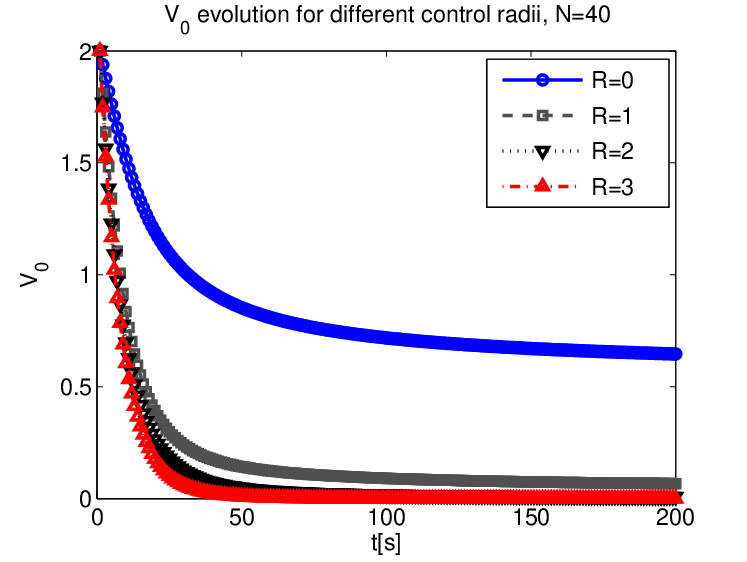
Local feedback control. The last test case studies the results presented in Section 5, where the feedback is computed according to the local average in eq.(22). Simulations in Figure 5 illustrate the setting. From an uncontrolled system, represented by a local feedback radius , by increasing this quantity, partial flocking is consistently achieved, until full consensus is observed for large radii mimicking a total information feedback control. From a theoretical perspective, this result is presented in Theorem 5.1, which describes a sufficient consensus region for feedback control based on local averages. This theorem recovers on its asymptotics previous results in [11], and [3], related to consensus regions for uncontrolled and fully controlled systems under total information feedback, respectively. It has been reported in the literature [4], that estimates for consensus regions such as the one provided by Theorem 2.1, are not sharp in many situations. In this direction, we proceed to contrast the theoretical consensus estimates with the numerical evidence. For this purpose, for a fixed number of agents, we span a large set of possible initial configurations determined by different values of . For every pair we randomly generate a set of 20 initial conditions, and we simulate for a sufficiently large time frame. We measure consensus according to a threshold established on the final value of ; we consider that consensus has been achieved if the final value of is lower or equal to . We proceed by computing empirical probabilities of consensus for every point of our state space ; results in this direction are presented in Figures 6 and 7. We first consider the simplified case of 2 agents; according to [3], for this particular case, the consensus region estimate provided by Theorem 2.1 is sharp, as illustrated is by the results presented in Figure 6. Furthermore, it is also the case for Theorem 5.1; for , the consensus region predicted by the theorem coincides with the numerically observed ones.
 |
 |
 |
 |
 |
 |
 |
 |
 |
 |
Figure 7 illustrates the case when a larger number of agents is considered. In a similar way as for Theorem 2.1, the consensus region estimate is conservative if compared with the region where numerical experiments exhibit convergent behavior. Nevertheless, Theorem 5.1 is consistent in the sense that the theoretical consensus region increases gradually as grows, eventually covering any initial configuration, which is the case of the total information feedback control, as presented in [3, Proposition 2]. The numerical experiments also confirm this phenomena, as shown in Figure 8 , where contour lines showing the probability of consensus for different radii locate farther from the origin as increases.
 |
 |
 |
 |
 |
 |

Concluding remarks and perspectives
We have presented a set of feedback controllers for consensus emergence in nonlinear multi-agent systems of Cucker-Smale type. The proposed control designs address different situations concerning leader-following configurations, stabilization under perturbed information, and decentralized, local feedback control. In general, we characterize consensus emergence in every case, providing a coherent extension of the available results in the literature. Furthermore, numerical experiments assess the performance of the controllers in a consistent way.
Among possible future directions of research, let us mention that numerical evidence suggest that sharper consensus estimates should be possible to be derived, if the structure of the internal dynamics is more intensively used in the computations. Another natural extension of our work would be to consider the consensus emergence problem, under a decentralized control computed via an optimality-based approach.
References
- [1] L. Bakule. Decentralized control: An overview. Annual Reviews in Control, 32(1):87 – 98, 2008.
- [2] M. Ballerini, N. Cabibbo, R. Candelier, A. Cavagna, E. Cisbani, I. Giardina, V. Lecomte, A. Orlandi, G. Parisi, A. Procaccini, M. Viale, and V. Zdravkovic. Interaction ruling animal collective behavior depends on topological rather than metric distance: Evidence from a field study. Proceedings of the National Academy of Sciences, 105(4):1232–1237, 2008.
- [3] M. Caponigro, M. Fornasier, B. Piccoli, and E. Trélat. Sparse Stabilization and Control of Alignment Models. to appear in Math. Mod. Meth. Appl. Sci. (M3AS), preprint: arXiv:1210.5739, 2012.
- [4] J. A. Carrillo, M. Fornasier, G. Toscani, and F. Vecil. Particle, kinetic, and hydrodynamic models of swarming. In G. Naldi, L. Pareschi, G. Toscani, and N. Bellomo, editors, Mathematical Modeling of Collective Behavior in Socio-Economic and Life Sciences, Modeling and Simulation in Science, Engineering and Technology, pages 297–336. Birkhäuser Boston, 2010.
- [5] F. Cucker and C. Huepe. Flocking with informed agents. MathS In Action, 1(1):1–25, 2008.
- [6] F. Cucker and S. Smale. Emergent behavior in flocks. IEEE Trans. Automat. Control, 52(5):852–862, 2007.
- [7] F. Cucker and S. Smale. On the mathematics of emergence. Jpn. J. Math., 2(1):197–227, 2007.
- [8] A. Filipov. Differential equations with Discontinuous Righthand Sides. Volume 18 of Mathematics and its Applications (Soviet Series). Kluwer Academic Publishers Group, Dordrecht, 1988.
- [9] M. Fornasier and F. Solombrino. Mean-field optimal control. to appear in ESAIM, Control Optim. Calc. Var., preprint: arXiv:1306.5913, 2013.
- [10] S.-Y. Ha, T. Ha, and J.-H. Kim. Asymptotic dynamics for the cucker–smale-type model with the rayleigh friction. Journal of Physics A: Mathematical and Theoretical, 43(31):315201, 2010.
- [11] S.-Y. Ha, T. Ha, and J.-H. Kim. Emergent behavior of a Cucker-Smale type particle model with nonlinear velocity couplings. IEEE Trans. Automat. Control, 55(7):1679–1683, 2010.
- [12] R. Hegselmann and U. Krause. Opinion dynamics and bounded confidence models, analysis, and simulation. Journal of Artificial Societies and Social Simulation, 5(3), 2002.
- [13] P. Ignaciuk and A. Bartoszewicz. Congestion Control in Data Transmission Networks. Springer, 2013.
- [14] R. M. Murray. Recent research in cooperative control of multivehicle systems. Journal of Dynamic Systems, Measurement, and Control, 129(5):571–583, 2007.
- [15] R. Olfati-Saber and R. Murray. Consensus problems in networks of agents with switching topology and time-delays. IEEE Trans. Autom. Control, 49(9):1520–1533, Sept 2004.
- [16] A. A. Peters, R. H. Middleton, and O. Mason. Leader tracking in homogeneous vehicle platoons with broadcast delays. Automatica, 50(1):64 – 74, 2014.
- [17] C. W. Reynolds. Flocks, herds and schools: A distributed behavioral model. SIGGRAPH Comput. Graph., 21(4):25–34, Aug. 1987.
- [18] T. Vicsek, A. Czirók, E. Ben-Jacob, I. Cohen, and O. Shochet. Novel type of phase transition in a system of self-driven particles. Phys. Rev. Lett., 75:1226–1229, Aug 1995.