Interacting scalar tensor cosmology in light of SNeIa, CMB, BAO and OHD observational data sets

Observational data sets including Cosmic Microwave Background(CMB) [1, 2], Supernovae type Ia (SNeIa) [3, 4], Baryonic Acoustic Oscillations (BAO) [5, 6], Observational Hubble Data (OHD) [7, 8], Sloan Digital Sky Survey (SDSS) [9, 10], and Wilkinson Microwave Anisotropy Probe (WMAP) [11, 12], are considered as criterion for accuracy of theoretical models. Amongst these constraints, the CMB and SNeIa( because of abundance of their data sources) attract more attention. It is notable, the SNeIa constraint in high redshift values do not give a good clue to investigate the evolution of the Universe. It is obvious the results of individual observations give different values for free parameters of a theoretical model; hence, it is better that, to estimate the best quantities for free parameters of the model one considers the whole of observational data sets including CMB, SNeIa, BAO and OHD. Therefore, this motivated us to study the behaviour of free parameters and their overlaps. Thence, a collective of observations including SNeIa, CMB, BAO and OHD are considered. Meanwhile the mentioned observational data sets have predicted an ambiguous form of matter which leads to an accelerated phase of present epoch and it is well known as dark energy. Based on this ambiguous form of matter, scientists have proposed different proposals up to now. Amongst all of those proposals, the cosmological constant, $\Lambda$, model attracts more attention [13, 14]. But this mechanism suffers two well known drawbacks. The first of them is related to estimate the contribution of quantum fluctuation of zero point energy and second is related to the ratio of $\Lambda$ and dark matter energy densities. These problems and also the excellent work by Brans and Dicke [15] motivated scientists to introduce a mechanism which $\Lambda$ had time dependency, namely quintessence [16, 17, 18]. Beside the quintessence mechanism, some proposals which risen from quantum gravity or string theory are introduced to estimate cosmological parameters. For instance one can refer to tachyon [19, 20], phantom [21, 22, 23], quintum [24, 25], k-essense [26, 27] and so on. Also some models which were risen from quantum field fluctuations or space time fluctuations attract more attention to investigate dark energy concept. For such models, one can mention Zero Point Quantum Fluctuations(ZPQF) [28, 29, 30], Holographic Dark Energy(HDE) [31, 32, 33, 34, 35, 36], Agegraphic Dark Energy (ADE) and new-ADE [37, 38, 39]. If scalar field, in the quintessence model couples to matter (non relativistic) it induces to appear a fifth force. When the coupling is of order unity, the results of strongly coupling scalar field is not in good agreement with local gravity tests (for instance in solar system). Thus a mechanism should be exist to suppress the effect of fifth force; such mechanism is capable to reconcile strong coupling models with local experiments was proposed by Khoury and Weltman [40, 41] and also, separately, by Mota and Barrow [42] namely chameleon. In this mechanism, one can not choose an arbitrary Lagrangian for matter, $L_{m}$. To avoid deviation of geodesic trajectory, the author of [43] has shown the best choices are $L_{m}=P$ and $L_{m}=-\rho$, where $P$ is pressure and $\rho$ is energy density of matter, for more discussion we refer reader to [44, 45, 46]. Therefore main motivation of this work is investigation the behavior of an interacting scalar field mechanism; based on these calculations and SNeIa, CMB, BAO and OHD data sets the minimum value of $\chi^{2}$ for the effective dark energy equation of state are achieved. The scheme of the paper is as follows:
The above discussions which are brief review about observational and theoretical motivations are considered as introduction. In Sec. 2, the general theoretical discussions risen from a chameleon like mechanism related to the cosmological parameters such as Hubble, deceleration and coincidence parameters will be discussed. In Sec. 3, a brief review about cosmological data sets are brought. In Sec. 4, the observational data sets including SNeIa, CMB, BAO and OHD are considered, to estimate the minimum value of $\chi^{2}$ related to free parameters of an ansatz for the effective dark energy equation of state. And at last, Sec. 5, is dedicated to concluding remarks.

In chameleon like scalar field scenario, the mass of scalar field is a function of local matter density, so that, it is sufficiently large on dense environment. Due to this fact, the equivalence principal (EP) is satisfied in the laboratory [40, 41]. In addition, the Brans Dicke $\omega$ parameter for two observational values of $\gamma$ post Newtonian parameter take the values of order $10^{4}$ [47], which satisfies the solar system constraint. The chameleon like scenario is defined as

$$S=\int{d^{4}x\frac{1}{2}\sqrt{-g}\Big({R-\partial^{\mu}\varphi\,\partial_{\mu}\varphi-2V(\varphi)+2f(\varphi)L}\Big)},$$

(1)

[43, 44, 48, 49, 50, 51, 52]. In this equation $g$ is the determinant of the metric, $V(\varphi)$ is a run away potential and the latest term indicates a non-minimal coupling between scalar field and matter sector. It should be noted $L$ is the Lagrangian density of matter which consists of both dark matter and dark energy sectors as perfect fluid [47, 48, 49, 52, 53]. It should be noticed that, background is a spatially flat Friedmann-Limatire-Robertson-Walker (FLRW) Universe, with signature $(+2)$. The variation of the action 1, with respect to (w.r.t) $g_{\mu\nu}$ results the gravitational field equation as

$$G_{\mu\nu}=f(\varphi)T_{\mu\nu}+T_{\mu\nu}^{(\varphi)},$$

(2)

where the stress-energy density of scalar field expresses

$$T_{\mu\nu}^{(\varphi)}=\left({\nabla_{\mu}\varphi\nabla_{\nu}\varphi-\frac{1}{2}g_{\mu\nu}(\nabla\varphi)^{2}}\right)-g_{\mu\nu}V(\varphi),$$

(3)

and

$$T_{\mu\nu}=\frac{{-2}}{{\sqrt{-g}}}\frac{{\delta(\sqrt{-g}L)}}{{\delta g^{\mu\nu}}},$$

(4)

is the definition of stress-energy tensor of matter. By considering $00$ and $ii$ components of $T^{(\varphi)}_{\mu\nu}$, the energy density and pressure could be achieved. After some algebra the conservation equation reads

$$\nabla_{\mu}(G^{\mu\nu})=\nabla_{\mu}\Big[f(\varphi)T^{\mu\nu}+T_{(\varphi)}^{\mu\nu}\Big]=0.$$

(5)

In addition, the variation of the action 1, w.r.t scalar field gives the evolution equation as

$$\ddot{\varphi}+3H\dot{\varphi}=-V(\varphi)+\frac{{\partial f(\varphi)}}{{\partial\varphi}}L.$$

(6)

Now, by substituting equation 6 into relation 5, two conservation equations for scalar field and matter are attained as

	$\displaystyle\nabla_{\mu}[T_{(\varphi)}^{\mu 0}]$	$\displaystyle=$	$\displaystyle\dot{f}(\varphi)L,$		(7)
	$\displaystyle\nabla_{\mu}[f(\varphi)T^{\mu 0}]$	$\displaystyle=$	$\displaystyle-\dot{f}(\varphi)L,$		(8)

where over $dot$ denotes derivation w.r.t ordinary cosmic time, $t$. As it was mentioned in the introduction, the Lagrangian of matter is considered as $L=L_{(m)}+L_{(de)}$, [52, 54]; where subscript $m$ denotes matter (cold dark matter and baryons) and $de$ refers to dark energy. Then the conservation equations could be rewritten as

	$\displaystyle\nabla_{\mu}\Big[f(\varphi)T_{(m)}^{\mu 0}\Big]$	$\displaystyle=$	$\displaystyle-\dot{f}(\varphi)L_{(m)},$		(9)
	$\displaystyle\nabla_{\mu}\Big[f(\varphi)T_{(de)}^{\mu 0}\Big]$	$\displaystyle=$	$\displaystyle-\dot{f}(\varphi)L_{(de)},$		(10)
	$\displaystyle\nabla_{\mu}\Big[T_{(\varphi)}^{\mu 0}\Big]$	$\displaystyle=$	$\displaystyle\dot{f}(\varphi)(L_{(m)}+L_{(de)}).$		(11)

By combining the relation 2 and above equations, it is easy to receive

$$\nabla_{\mu}\Big[T_{(\varphi)}^{\mu 0}+f(\varphi)T_{(de)}^{\mu 0}\Big]=\dot{f}(\varphi)L_{(m)}.$$

(12)

In the next step, by virtue of the definition of $T_{\mu\nu}^{(\varphi)}$ and equation 2, the Einstein tensor is modified as

$$G^{\mu\nu}=f(\varphi)\Big[{T_{(m)}^{\mu\nu}+T_{(de)}^{\mu\nu}+\frac{1}{{f(\varphi)}}T_{(\varphi)}^{\mu\nu}}\Big].$$

(13)

Hereafter, we postulate that both scalar field and dark energy, behave the same as perfect fluid, thence for such perfect mixture the effective stress-energy tensor is obtained as follows

$$T_{(DE)}^{\mu\nu}=T_{(de)}^{\mu\nu}+\frac{1}{{f(\varphi)}}T_{(\varphi)}^{\mu\nu},$$

(14)

where subscript $DE$ denotes effective dark energy. Therefore using equations 7-14, the modified Einstein equation and conservation relations are attained as

$$G^{\mu\nu}=f(\varphi)\Big[T_{(m)}^{\mu\nu}+T_{(DE)}^{\mu\nu}\Big],$$

(15)

	$\displaystyle\nabla_{\mu}\Big[f(\varphi)T_{(m)}^{\mu 0}\Big]$	$\displaystyle=$	$\displaystyle-\dot{f}(\varphi)L_{(m)},$		(16)
	$\displaystyle\nabla_{\mu}\Big[f(\varphi)T_{(DE)}^{\mu 0}\Big]$	$\displaystyle=$	$\displaystyle\dot{f}(\varphi)L_{(m)}.$		(17)

It should be noticed that, in the right hand side of above equations, only $L_{(m)}$ is appeared. In fact it could be concluded that the energy, for different components of the Universe is not conserved separately. In refs.[55, 56, 57], it has been shown that, for perfect fluids, that do not couple directly to the other components of the Universe, there are different Lagrangian densities are equivalent. Namely, one can find that the two Lagrangian densities $L_{(m)}=P$ and $L_{(m)}=-\rho$ give the same stress-energy tensor and the equation of motions for all components of the system are similar as well. But in an interacting case, which matter has an interaction with scalar field, the Lagrangian degeneracy is broken. Based on ref.[43], the best choice for such models is $L_{(m)}=P$. Using this definition for Lagrangian of the matter one can obtain

$$H^{2}=\frac{1}{3}f(\varphi)\Big[\rho_{m}+\rho_{DE}\Big],$$

(18)

and also

	$\displaystyle\frac{d}{{dt}}\Big[f(\varphi)\rho_{m}\Big]+3Hf(\varphi)\rho_{m}=0,$		(19)
	$\displaystyle\frac{d}{{dt}}\Big[f(\varphi)\rho_{DE}\Big]+3Hf(\varphi)\Big[1+\omega_{DE}\Big]\rho_{DE}=0,$		(20)

where $H=\dot{a}(t)/a(t)$ is the Hubble parameter, $a(t)$ is scale factor and $\omega_{DE}$, is the EoS parameter of the effective dark energy and satisfies EoS equation as

$$P_{DE}=\omega_{DE}\times\rho_{DE}.$$

(21)

To establish an accurate link between theoretical results and observations, one can use the red shift parameter, $z$, instead of the scale factor; these two cosmological parameters have a relation as

$\displaystyle\frac{{a(t_{0})}}{{a(t)}}=1+z\,\qquad\dot{z}=-(1+z)H.$

(22)

Thus substituting equation 22 into 19 and 20, one finds out

	$\displaystyle f(\varphi)\rho_{m}=f_{0}\times\rho_{m0}\times(1+z)^{3},$		(23)
	$\displaystyle f(\varphi)\rho_{DE}=f_{0}\times\rho_{DE0}\times\exp\Big[\int_{0}^{z}{3\frac{{1+\omega_{DE}(\tilde{z})}}{{1+\tilde{z}}}d\tilde{z}}\Big],$		(24)

where $\rho_{DE0}$ and $\rho_{m0}$ refer to energy densities of dark energy and matter at present time, respectively.

In this section, we should emphasis that the analysis is restricted to the background level, and do not include perturbations. In the following, we want to compare our theoretical results with observations. To this end, we consider four important data sets including SNeIa, CMB, BAO and OHD. In some papers, it was claimed OHD, which obtained versus red shift, is comparable with SNeIa data set, for instance we refer reader to reference [7] and references which are there. This subject motivated us to investigate the effects of this new data set beside other observations to improve the theoretical results. As it will be discussed, the results of OHD although is not independent of SNeIa and BAO data sets [7] but has not any dependency to CMB. Also there are two ways to study CMB and BAO data point among the full parameter distribution and Gaussian which in follow the latter will be used.

As it was mentioned, we have introduced an ansatz as equation 36, that consist of three free parameters. Where $\omega_{1}$ indicates present time value of $\omega_{DE}$. For more convenience we can suppose $\omega_{\rm{0}}=f_{0}=1$ and therefore Eq.(36) is reduced to [54, 58]

$\displaystyle\omega_{DE}(z)=\omega_{1}(1+z)^{\beta}.$

(57)

Also, the mean square of relative error functions $\chi^{2}$, normally cause the free parameters plane split in two parts. People usually are interested to the regions which $\chi^{2}/N\leq 1$, where $N$ denotes the amount of observational data. Whereas we use $Union-2$ data set for SNeIa, $N$ for supernovae is $N_{SNe}=557,$ and also for OHD, CMB and BAO, one has $N_{OHD}=28$, $N_{CMB}=1$ and $N_{BAO}=1$. Since in this work three free parameters are appeared, the space of constraints has three dimensions. Thence for better expression, one can map figures on two dimensions (in fact it is supposed that, the free parameters are independent) and their values will be analyzed. The common regions for best fitting of all constraints, play key role in this study. Based on above discussions we plot a couple of free parameters in Figures 4 - 6. In Figure 4 we investigate the constraints on $\Omega_{m0}$ in $\omega_{1}\,\beta$ plate, and also for two constraints SNeIa and OHD minimum points of $\chi^{2}$ are distinguished. In Figures 5 using best value of $\omega_{1}$, the constraints in $\Omega_{m0}\,\beta$ are obtained, in a similar way for best value of $\beta$, the behavior of constraints in $\omega_{1}\,\Omega_{m0}$ surface will be shown. Let us, return our attention to figure 4 again. For $\Omega_{m0}=0.2$, the CMB, BAO and OHD have an overlap region, but they are not in agreement with SNeIa results. Also for a different quantity, the SNeIa and OHD results could be in agreement with together. This different behavior of constraints indicates that if one wants to compare theoretical results with observations, it is better the greatest set of constraints, to be considered. For more investigation about overlaps and the effects of individual observations, we plot figures 7 and 8. In figure 7 the behaviour of $\chi_{\rm T}^{2}=\chi_{\rm{SNe}}^{2}+\chi_{\rm{OHD}}^{2}+\chi_{\rm{CMB}}^{2}+\chi_{\rm{BAO}}^{2}$ and $\chi_{\rm T}^{2}=\chi_{\rm{SNe}}^{2}+\chi_{\rm{CMB}}^{2}+\chi_{\rm{BAO}}^{2}$ for $\Delta\chi_{\rm T}^{2}=3.53,6.25,8.02$ are compared. Also in figure 8 to investigate degeneracy one can consider $\chi_{\rm T}^{2}=\chi_{\rm{SNe}}^{2}+\chi_{\rm{OHD}}^{2}+\chi_{\rm{CMB}}^{2}+\chi_{\rm{BAO}}^{2}$ and $\chi_{\rm T}^{2}=\chi_{\rm{OHD}}^{2}+\chi_{\rm{CMB}}^{2}+\chi_{\rm{BAO}}^{2}$ for $\Delta\chi_{\rm T}^{2}=0.1,0.2,0.3$. These two figures indicate that although the importance of individual OHD data surveying (in comparison SNeIa, CMB and BAO) is not so important, but it decreases the degeneracy between free parameters of the model. From figures 7 and 8, it is obvious that a collective of four constraints has completely different results in comparison to even three constraints. In the following, by means of observations, we use some custom quantities which are considered for better estimation of theoretical parameters of the model. Since all free parameters of the model are independent, the total likelihood function could be introduced as

$\displaystyle{\cal L}_{\rm{T}}={\cal L}_{{\rm{SNe}}}\times{\cal L}_{{\rm{OHD}}}\times{\cal L}_{{\rm{CMB}}}\times{\cal L}_{{\rm{BAO}}},$

(58)

therefore the total $\chi^{2}$ function could be achieved as

$\displaystyle\chi_{\rm{T}}^{2}=\chi_{{\rm{SNe}}}^{2}+\chi_{{\rm{OHD}}}^{2}+\chi_{{\rm{CMB}}}^{2}+\chi_{{\rm{BAO}}}^{2}.$

(59)

It is considerable to attain the maximum amount of the probability and the minimum value of $\chi^{2}$, we should minimize $\chi_{\rm{T}}^{2}$. Also it should be noted, in 59 all components have same weight. So the likelihood method is equivalent to this fact that, for instance all measurements which lead to CMB is equal to a supernova explosion!. Afterwards we return to this problem. Another quantity which could be used for data fitting process is

$$\tilde{\chi}^{2}=\frac{\chi_{T}^{2}}{N_{dof}}$$

(60)

where subscript $dof$ is abbreviation of degree of freedom, and $N_{dof}$ could be defined as the difference between all observational sources and the amount of free parameters. Let’s explain it in more detail, whereas the amounts of all observations are $557+28+1+1=587$, and the number of free parameters are $4$, by considering $H_{0}$, therefore $N_{dof}$, is equal to $583$. Also one knows, the acceptable quantity for $\tilde{\chi}^{2}$ is $1.05$. For more convenient, we now define the average relative error functions as follows

	$\displaystyle\bar{\chi}_{{\rm{SNe}}}^{2}=\frac{{\chi_{{\rm{SNe}}}^{2}}}{{N_{{\rm{SNe}}}}},$		(61)
	$\displaystyle\bar{\chi}_{{\rm{OHD}}}^{2}=\frac{{\chi_{{\rm{OHD}}}^{2}}}{{N_{{\rm{OHD}}}}},$		(62)
	$\displaystyle\bar{\chi}_{{\rm{CMB}}}^{2}=\frac{{\chi_{{\rm{CMB}}}^{2}}}{{N_{{\rm{CMB}}}}},$		(63)
	$\displaystyle\bar{\chi}_{{\rm{BAO}}}^{2}=\frac{{\chi_{{\rm{BAO}}}^{2}}}{{N_{{\rm{BAO}}}}}.$		(64)

Finally we can introduce $\chi_{\rm m}^{2}$ function, which is equal to maximum of $\bar{\chi}^{2}$ functions and it could be considered as

$\displaystyle\chi_{\rm{m}}^{2}={\rm{max}}\,{\rm{of}}\,\left({\bar{\chi}_{{\rm{SNe}}}^{2},\bar{\chi}_{{\rm{OHD}}}^{2},\bar{\chi}_{{\rm{CMB}}}^{2},\bar{\chi}_{{\rm{BAO}}}^{2}}\right).$

(65)

In fact the $\chi_{\rm m}^{2}$ function could be considered as a criterion of accuracy for the models. Now we want to compare the behavior of $\chi_{\rm m}^{2}$ and $\tilde{\chi}^{2}$ functions. Without loss the generality of the model, one can plot the three dimensional shape of $\chi_{\rm m}^{2}$ and $\tilde{\chi}^{2}$, versus free parameters of the model. These diagrams help us to find out the best estimation of the free parameters in comparison to observations; for more clarity one can see the figure 9. In this figure, the first diagram shows the minimum of $\chi_{\rm m}^{2}$ and $\bar{\chi}^{2}$ versus $\Omega_{m0}$. Also in two latest diagrams of figure 9, the minimum points are drown based on $\omega_{1}$ and $\beta$ respectively. By comparison the behavior of these relative error functions in Figure 9 one can realize that, there are more points (or neighborhood) in which $\tilde{\chi}^{2}<1$, but $\chi_{m}^{2}$ exceeds $1.05$. In fact this behavior was predictable, because in definition of $\tilde{\chi}^{2}$, we use the contribution of all observational data set. So, for example the $\chi_{{\rm{CMB}}}^{2}$ deviation of best fitting results, could be recompense by SNeIa data abundance. We will return to this drawback, after some discussion about likelihood and relative error functions. For more illustration, we portrait the different surfaces of three dimensional, $(\Omega_{\rm{m0}},\omega_{\rm{1}},\beta)$, to $(\Omega_{\rm{m0}},\beta)$, $(\omega_{1},\Omega_{\rm{m0}})$ and $(\omega_{1},\beta)$ surfaces, which are brought in Figures 10, 11 and 12. Diagrams $B$ and $C$ are related to $(\chi_{\rm T}^{2})_{\rm{min}}$, where the subscript $min$, shows the minimum value of $\chi_{{\rm{T}}}^{2}$ . It is notable, in a three dimensional space of free parameters, the confidence levels $68.3\%$, $90\%$ and $95.4\%$ are proportional to $\Delta\chi_{\rm T}^{2}=3.53$, $\Delta\chi_{\rm T}^{2}=6.25$ and $\Delta\chi_{\rm T}^{2}=8.02$ surfaces respectively where $\Delta\chi_{\rm T}^{2}=\chi_{\rm T}^{2}-(\chi_{\rm T}^{2})_{\rm{min}}$. In diagram $B$ of Figures 10, 11 and 12 the counter lines of confidence levels are drown and in diagram $C$, both the $\chi_{\rm m}^{2}$ surfaces and counter lines are brought for more comparison. From diagram $C$ it is realized that the confidence level counters exceed the $\chi_{\rm m}^{2}$ regions. From this behaviour it is concluded that, the theoretical prediction of CMB shift parameter is very greater than it’s observational quantity. As mentioned heretofore, when the total mean square error function is introduced the weight of all constraints was identical and this causes some problems. As a matter of fact, the results of likelihood’s parameter, equation 59, the effect of CMB shift parameter in comparison to the abundant SNeIa data set is ignored. For more information, one can see Table 2 and definition of $N_{dof}$. To overcome these problems, we redefine $\chi_{\rm{T}}^{2}$ as bellow

$\displaystyle\chi_{\rm{T}}^{2}=\chi_{{\rm{SNe}}}^{2}+\chi_{{\rm{OHD}}}^{2}+3\,\chi_{{\rm{CMB}}}^{2}+3\,\chi_{{\rm{BAO}}}^{2}.$

(66)

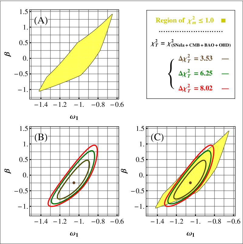
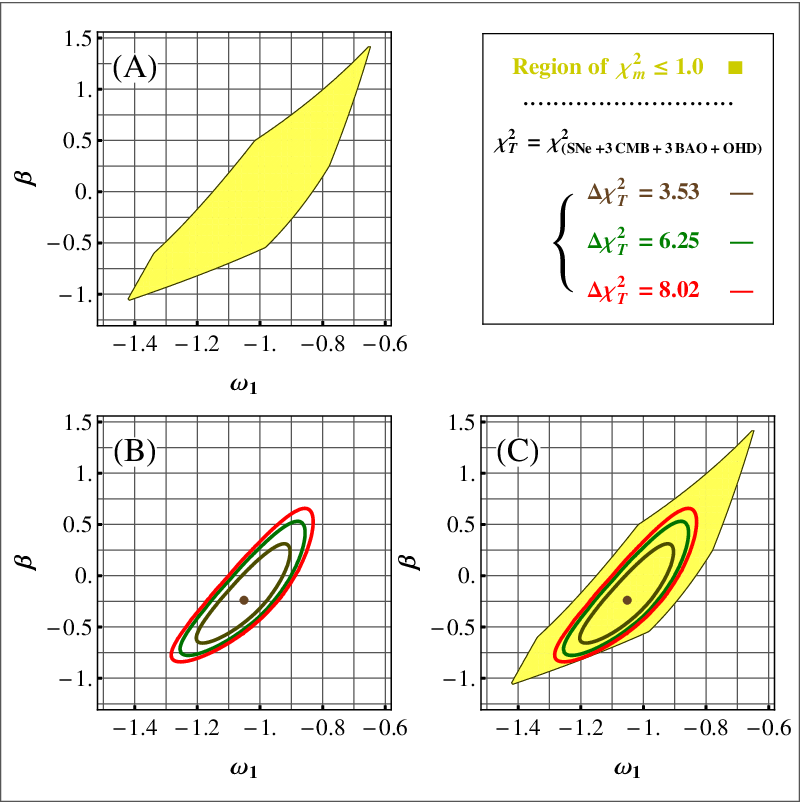
It should be noted, in data fitting and maximization of probability quantities these two definitions of $\chi_{\rm T}^{2}$, i.e. equations 59 and 66, have not very different. For justifying this claim one can compare Tables 2 and 3 which are related to 59 and 66 respectively. But in figures which related to confidence levels one can observe that the exceeding of confidence levels are reduced, therefore the re-weight of some constraints can improve the behaviour of the model. For more clarification one can refer to figures 13, 14 and 15. Now by means of 66, we margin the likelihood $\mathcal{L}(\Omega_{\rm{m0}},\omega_{1},\beta)$ w.r.t $\omega_{1}$, $\beta$ and $\Omega_{\rm{m0}}$ respectively. Also the relative probability functions $\mathcal{L}(\Omega_{\rm{m0}},\beta)$, $\mathcal{L}(\omega_{1},\Omega_{\rm{m0}})$ and $\mathcal{L}(\omega_{1},\beta)$ in two dimensional confidence levels $68.3\%$, $90\%$ and $95.4\%$ are plotted in Figure 16. For more investigations, we will draw the one dimensional marginalized likelihood functions $\mathcal{L}(\Omega_{\rm{m0}})$ versus $\Omega_{\rm{m0}}$, $\mathcal{L}(\omega_{1})$ based on $\omega_{1}$ and $\mathcal{L}(\beta)$ versus $\beta$ in figure 17. Meanwhile in Table 4 one observes the quantities which maximize the marginalized likelihoods using different confidence levels by means of confidence levels $\sigma_{1}=68.3\%$ and $\sigma_{2}=95.4\%$ .