Asymptotically free scaling solutions in nonabelian Higgs models
Abstract
We construct asymptotically free renormalization group trajectories for the generic nonabelian Higgs model in four-dimensional spacetime. These ultraviolet-complete trajectories become visible by generalizing the renormalization/boundary conditions in the definition of the correlation functions of the theory. Though they are accessible in a controlled weak-coupling analysis, these trajectories originate from threshold phenomena which are missed in a conventional perturbative analysis relying on the deep Euclidean region. We identify a candidate three-parameter family of renormalization group trajectories interconnecting the asymptotically free ultraviolet regime with a Higgs phase in the low-energy limit. We provide estimates of their low-energy properties in the light of a possible application to the standard model Higgs sector. Finally, we find a two-parameter subclass of asymptotically free Coleman-Weinberg-type trajectories that do not suffer from a naturalness problem.
I Introduction
While the naturalness problem has been a dominant paradigm for model building beyond the standard model of particle physics, the triviality problem of the Higgs sector conceptually appears much more severe as it inhibits a constructive ultraviolet (UV)-complete definition of the standard model as an interacting quantum field theory. The triviality of the standard model Higgs sector is expected to arise from the fundamental scalar degrees of freedom. For pure scalar theories, strong evidence for triviality [1] – the fact that the continuum limit can only be taken for the noninteracting theory – has been accumulated by lattice simulations in [2] and analytic methods [3] (see [4] for a rigorous proof in ). For nonabelian Higgs models, Monte-Carlo methods [5] have found no indication for continuous phase transitions facilitating a nontrivial continuum limit. In practice, triviality arguments have been used to put upper bounds on the Higgs mass [6] long before its discovery.
Since ATLAS and CMS have found a comparatively light scalar boson [7], the standard model appears to be in a “near-critical” regime [8, 9] indicating that the Higgs self-interaction is small near the Planck scale. This would be natural if all standard-model interactions including the scalar self-interaction were asymptotically free (AF) [10]. This is, however, not the case from the standard viewpoint of perturbative functions.
The construction of AF Yang-Mills-Higgs(-Yukawa) systems is in principle straightforward on the basis of a perturbative analysis [11, 12, 13, 14, 15, 16]. In particular, the problematic quartic scalar interaction , can be marginal-relevant (UV stable) or -irrelevant (UV unstable), depending on the model and the choice of trajectories. UV-complete trajectories which emanate from the Gaußian fixed point (FP) can also be built by fixing the unstable marginal-irrelevant direction. In RG-improved perturbation theory, this scenario requires additional fermions as well as eigenvalue conditions [12, 13] to be satisfied [17]. This implies a reduction of couplings [18], here effectively removing one parameter, as is then purely induced, implying a prediction of the Higgs-to--boson mass ratio. To our knowledge none of such theories comes sufficiently close to the standard model. Alternatively, UV completion in Higgs models can be achieved via asymptotic safety, which also requires dynamical fermions [19].
In this Letter, we consider the construction of AF Yang-Mills-Higgs systems from a new viewpoint. Our central idea is that, in order for suitable AF nonabelian Higgs models to exist, the scalar potential needs to approach absolute flatness concurrently with the vanishing gauge coupling . This permits large amplitude fluctuations of the scalar field controlled by the latter parameter. We thus suggest to consider gauge-rescaled scalar field variables , with some power , as the relevant measure for amplitudes. While at this point merely seems to be an unphysical rescaling parameter, we show that it parametrizes RG-scale-dependent boundary conditions for the effective potential. These in turn are equivalent to -dependent renormalization and boundary conditions for the correlation functions of the theory. As a consequence, parametrizes a set of physically distinct RG flows, each one possessing a Gaußian FP and allowing for AF trajectories.
First signatures of such a trajectory have been found in a gauged Yukawa model in [20]. In the present work, we explore the general pattern to construct UV-complete trajectories for AF nonabelian Higgs models, including the physically relevant SU(2) model, for the first time.
II A perturbative illustration
Let us start by recalling the standard perturbative analysis of a nonabelian Higgs model, as presented, e.g., in [11]. The one-loop -functions derived under the standard assumption of working in the deep Euclidean region, where the RG scale is much larger than any other mass scale, read
| (1) |
The integrated flow in this simple truncation yields
| (2) |
with and , and is an integration constant. For the SU(2) model,
such that is negative and the flow in Eq. (2) has a branch cut, the position of which depends on and . This is the so-called Landau pole, indicating the unbounded increase of towards the UV and thus the failure of perturbation theory. This is considered as reflecting the triviality problem of the theory which is assumed to persist also beyond perturbation theory. If were positive, would simply be proportional to itself for sufficiently small with a -independent proportionality constant. In the limit , two special trajectories would appear, corresponding to solutions of the FP equation for the ratio [11]
| (3) |
and they would describe the possible UV asymptotics of all AF trajectories. Conversely, if at least one of these roots is positive, then there are AF trajectories in the positive plane. Nonabelian Higgs models with this property have been classified, e.g., in [14]. The standard SU(2) model is not of this type.
In order to explore possible loop holes of this conventional perturbative argument, let us study more general potentials of the form
| (4) |
This includes a possible vacuum expectation value and higher-order operators such as which can be used to effectively resum higher loop contributions. A nonperturbative way to study the flow of general potentials will be used below. Here, we simply study the contribution of to the flow of . Expressed in terms of , we find (),
| (5) |
In contrast to Eq. (3), this equation gives rise to a finite FP value for if the ratio stays finite and nonvanishing. Note that can have either sign, as long as the full potential including higher order terms stays bounded from below. If realized, this implies that and (and possibly all higher ) are asymptotically free together with the gauge coupling .
Perturbatively, it might seem difficult to stabilize in this way. However, there is an effect which is missed by the conventional perturbative analysis: to see this, let us study the flow of the minimum of the potential (ignoring wave function renormalizations for the moment),
| (6) |
For any positive , the ratio is attracted to a positive UV fixed point. This implies that can be attracted towards a UV fixed point potential in the regime of spontaneous symmetry breaking (SSB), such that the minimum increases proportional to the RG scale, .
This conclusion has a dramatic consequence: the standard assumption that the UV behavior of the theory can be exhaustively analyzed in the deep Euclidean region with any other scale can be violated. In order to explore the implications, we have to use a more powerful formalism that does not rely on the deep Euclidean limit, can deal with corresponding threshold effects as well as with the RG flow of full potentials .
Using the functional RG, we show below that the AF scenario visible in Eqs. (5), (6) is indeed realized and can be controlled in a weak-coupling analysis – though fully accounting for threshold effects. The scalar couplings run with the gauge coupling to zero towards the UV, with the ratios of the type being fixed by a boundary condition for the RG flow of the full potential . In fact, we find a three-parameter family of such RG trajectories. The flow of the above example with (e.g., ) and threshold effects included, i.e., at its fixed point, is shown below in Fig. 2.
III RG flow of the model
We concentrate on nonabelian Higgs models with a fundamental scalar as a key building block of the standard model of electroweak interactions; we consider gauge groups SU(), using the standard model SU(2) for concrete examples. This model includes a Yang-Mills sector with the field strength derived from the vector potential , and a minimally coupled scalar sector with a scalar potential that depends on the invariant . In this work, we analyze the RG flow not only restricted to the set of perturbatively renormalizable operators, but include a full scalar potential. Even if the higher operators turn out to be irrelevant and strongly suppressed along AF trajectories, it is crucial for the UV construction of these trajectories to go beyond the single-coupling analysis. We study the flow of a scale-dependent effective action
| (7) |
where . Here, all wave function renormalizations , the coupling , and the potential depend on a RG scale . The RG function(al)s for these quantities have been computed in [20], using the Wetterich equation [21, 22]. This formulation of the functional RG is useful as it makes no assumptions about the magnitude of the running masses and couplings, and incorporates dynamically generated thresholds. The relevance of the latter for UV completeness has first been studied in [23].
Using the background-field formalism, the running of the renormalized gauge coupling is linked to that of the wave function renormalization [24],
| (8) |
The present ansatz for the effective action yields the standard one-loop running, amended by threshold effects owing to gauge bosons and the Higgs scalar acquiring masses in the broken regime. Similarly, the scalar anomalous dimension exhibits a standard one-loop form including threshold effects [20].
Our search strategy for asymptotic freedom generalizes the preceding perturbative illustration by looking for trajectories such that the coupling vanishes as in the UV, with arbitrary power . The example given above corresponds to . The nontrivial asymptotic value for can be observed by rescaling the scalar field
| (9) |
such that plays the role of a natural renormalized dimensionless field. For the full scalar potential, we demand that higher couplings vanish in the UV with corresponding or higher powers of . The dimensionless effective potential
| (10) |
should then stay finite and non-vanishing in the far UV (the dimensionless quantities and are often used in the functional-RG literature).
The flow equation for this rescaled effective potential reads [20],
| (11) | |||||
where the scheme-dependent threshold functions encode the decoupling of massive modes. Using the linear regulator [25], we have and analogously for upon replacing by . The gauge-boson mass parameters arise from the eigenvalues of , e.g., for SU(2) for any .
Standard perturbative results are, of course, contained in Eq. (11): an expansion to order yields the universal one-loop function of Eq. (3) upon (i) ignoring RG improvement, inside the threshold functions, and (ii) taking the deep Euclidean limit, i.e., ignoring threshold effects after the expansion in . Similarly, the additional terms in Eq. (5) are derived by including this operator in the ansatz for the potential. Projecting onto the flow of the minimum leads to Eq. (6) in the limits (i) and (ii). We emphasize that many of our new results are not fully visible or remain hidden in this conventional perturbative limit.
IV Fixed points and scaling solutions
Let us first search for scaling solutions, which correspond to FPs of the RG flow, representing candidates for asymptotic limits of AF trajectories. For this, we consider Eq. (11) in the limit , but keeping and finite. The latter facilitates to consider boundary conditions for the effective potential, and thus for correlation functions, which are unapparent in conventional perturbation theory. Since the scalar loops in the last line approach irrelevant constants for , and the anomalous dimensions also approach zero asymptotically, the flow equation for becomes a first-order differential equation. The behavior of the gauge-boson-loop in the second line, depends on the value of . For , it approaches zero () or an irrelevant constant () and hence can be ignored. Therefore, for any regulator and any SU(), the FP solutions to the remaining part of the first line of Eq. (11) satisfying read
| (12) |
for a generic (irrelevant constants in are ignored). For , the gauge loop contributes nontrivially to the effective potential. For SU(2), we find using the linear regulator
| (13) |
with arbitrary. The precise functional form is regulator dependent, but any regulator yields this Coleman-Weinberg-type shape. For , the potential is bounded from below and has a nontrivial minimum . For , the minimum is at infinity.
The FP potentials of Eqs. (12,13), once re-expressed in terms of the original fields , provide the simplest portrait of a two-parameter family of asymptotically free solutions. Different values of correspond to different flows in coupling space. This translates into different -dependent boundary conditions for integrating the RG equation for . Near the FP, the trajectories differ from Eqs. (12,13) by higher powers of the gauge coupling. The trajectories can systematically be constructed in a weak-coupling expansion by expanding in powers of , and computing the potential for which this approximate functional vanishes. This procedure is justified by the stability analysis given below.
For the next-order approximation includes a linear term in the leading power of . The leading power is for , and for . The corresponding effective potentials are in the SSB regime
For or the position of the minimum is independent ( and respectively), whereas for it is proportional to and thus running to infinity in the UV. For , we solve the corresponding equation numerically. The resulting potential as a function of the unscaled field is shown in Fig. 1. Again, the minimum of approaches infinity in the UV, and the curvature at the minimum vanishes like .
While our analysis fully remains in the weak-coupling regime, our scaling solutions evade the triviality problem already signalled by conventional perturbation theory because of nontrivial threshold phenomena: since the scaling potentials have non-trivial minima which are finite in dimensionless units or even diverge with , the threshold effects remain relevant also in the UV. Thus the deep Euclidean region which is convenient for a standard perturbative analysis is incapable of properly accounting for the present scaling solutions.

For , logarithms slightly complicate the weak-coupling expansion. By taking the full gauge loop into account, analytical forms for the scaling solutions can be found which will be given elsewhere [26]
Let us now perform a stability analysis of these trajectories, taking advantage of their asymptotic description in terms of FPs of the RG flow of . For small gauge coupling, perturbations about these trajectories are translated into deviations from the FP, with components and . Since is proportional to , any eigenperturbation with non-vanishing gauge coupling must be marginal-relevant. Indeed the -dependent potential determined above is by construction a parametrization of the marginal-relevant eigendirection, since its flow is frozen apart from the running of . Conversely, any non-marginal eigenperturbation must have a vanishing component. At , the eigenvalue problem simplifies to the Gaußian one, for which the eigenperturbations are simple powers, . This includes a relevant () and a marginal direction (). Beyond the linear analysis, the direction is actually marginal-irrelevant, as is familiar from perturbation theory. This is visible in the stream-plot of Fig. 2 where the green (thick) line is the projection of a -asymptotically free trajectory onto the plane. We emphasize that all our effective potentials are polynomially bounded, exhibit self-similar eigenperturbations and thus satisfy standard RG requirements [27].
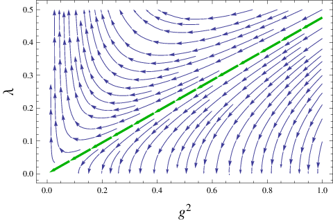
To summarize, we have identified new AF trajectories in the nonabelian Higgs model. In addition to the standard mass-type relevant deformation, we have provided the approximate parametrization of one marginal-relevant eigenperturbation for each pair . For UV-complete trajectories, the marginal-irrelevant -type perturbation is zero. Therefore, once a specific UV asymptotic behavior is determined by , only one physical parameter remains apart from an absolute scale. This is one parameter less than in usual perturbative scenarios. Yet, we gained the two positive parameters and , labeling different AF trajectories.
V Mass spectrum
The preceding analysis investigated the UV behavior of the AF trajectories in the nonabelian Higgs model. In order to explore the long range mass spectrum, we have to integrate the flow of the effective potentials towards the IR. If the trajectories end in a SSB phase, a Fermi scale and gauge boson and Higgs masses are generated. Trajectories emanating from a given fixed-point theory specified by and consist of the corresponding marginal-relevant eigenperturbation (parametrized by the gauge coupling ) possibly superimposed by a finite component of the relevant direction (the Gaußian perturbation) with some coefficient at a UV scale . Inspired by the standard model hierarchy, we assume to be very small, such that the system will spend a long RG time on top of the marginally relevant trajectory, establishing a large hierarchy . At a cross-over (CO) scale the relevant component sets in and drives the system away from the marginal-relevant trajectory. In practice, the initial conditions , at can be traded for , to be specified at (in the standard model, TeV).
For a simple estimate (blind to nonperturbative bound-state effects [28]) of the mass spectrum, we initialize the flow at with a potential that is equal to the analytic parameterization of the marginal perturbation obtained in the previous section, plus a relevant component, . We then evolve the full RG flow from down to . At the Fermi scale, the gauge coupling as well as the dimensionful conventionally-renormalized vev and mass parameters , in -units, will depend only on , , and for sufficiently big because of universality. We choose such that acquires a standard-model-like value; since the gauge running is logarithmically slow, and do not differ significantly. The parameter should be chosen sufficiently small in order to justify that it is ignored above , but also sufficiently large in order to drive the system rapidly into the SSB regime; in practice, was used for our estimates. For the running below , we approximate the full effective potential by a standard polynomial expansion about its minimum; order- polynomials turned out to be sufficient.
The Higgs-to-gauge boson mass turns out to be an increasing function of , which is approximately linear, at least for small-enough , . The slope depends on and decreases for larger . This suggests that any desired physical value of the mass ratio corresponds to a one-dimensional section through the plane, spanning the set of AF theories. Comparing the IR results at the Fermi scale to the initial values at , we find that the flow towards the IR essentially preserves the mass ratio already set by the initial condition at . In our scans we observed an almost -independent ratio of about one order of magnitude.
Let us finally explore the physical properties of Coleman-Weinberg-like trajectories which are defined as those with a zero relevant component [29]. We use an order- polynomial truncation and integrate the flow by keeping fixed the ratio between and a suitable power of , which determines the parameters . To reduce errors, we numerically solve the truncated finite- FP equations for including subleading corrections to the analytic formulas given above. We observe that these Coleman-Weinberg-like trajectories end in the SSB phase in the IR only if the gauge coupling at initialization is smaller than a critical -dependent value. The resulting Higgs-to-gauge boson mass parameter ratio is then a function of . For instance in the case, freeze-out occurs when the quartic coupling is still in the FP regime, such that the UV relation is preserved.
We emphasize that the measured value of the Higgs boson mass can be understood as essentially driven by top fluctuations [30, 31, 8, 32]. The small Higgs masses (ignoring bound-state effects [28]) in the pure nonabelian Higgs model along Coleman-Weinberg trajectories thus appear to fit the requirements of a realistic model. These trajectories may also be useful to construct a natural large hierarchy in the standard model via the Higgs portal [33]; in such a scenario, our nonabelian Higgs model could play the role of a UV-complete hidden sector.
In summary, we have discovered a three-parameter family of AF nonabelian Higgs models. Our results rely on a controlled weak-coupling analysis. Nevertheless, a conventional perturbative analysis in the deep Euclidean region is blind to these new trajectories as they arise from threshold phenomena which require a resummation to become visible in perturbation theory. If usable in the context of the full standard model or GUTs, our RG trajectories do not suffer from triviality and thus are candidate building blocks for a UV-complete quantum field theory. A two-parameter subset of Coleman-Weinberg-like AF trajectories is even free from the naturalness problem. We expect these trajectories to be directly accessible to lattice methods: simulations with bare potentials along the marginal-relevant eigenperturbations should lie on a line of constant physics. Still, rather large lattices may be necessary to resolve the Fermi scale as well as the crossover to the asymptotic regime.
Acknowledgements.
We thank Jörg Jäckel, Axel Maas, Gian Paolo Vacca and Christof Wetterich for interesting discussions, and Stefan Rechenberger, René Sondenheimer, and Michael Scherer for collaboration on related projects. We acknowledge support by the DFG under grants No. GRK1523/2, and Gi 328/5-2 (Heisenberg program).References
- [1] K. G. Wilson and J. B. Kogut, Phys. Rept. 12, 75 (1974);
- [2] M. Luscher and P. Weisz, Nucl. Phys. B 295, 65 (1988); Nucl. Phys. B 318, 705 (1989); A. Hasenfratz, K. Jansen, C. B. Lang, T. Neuhaus and H. Yoneyama, Phys. Lett. B 199, 531 (1987); U. M. Heller, H. Neuberger and P. M. Vranas, Nucl. Phys. B 399, 271 (1993) [arXiv:hep-lat/9207024]; U. Wolff, Phys. Rev. D 79, 105002 (2009) [arXiv:0902.3100 [hep-lat]]; . P. V. Buividovich, Nucl. Phys. B 853, 688 (2011) [arXiv:1104.3459 [hep-lat]].
- [3] O. J. Rosten, JHEP 0907, 019 (2009) [arXiv:0808.0082 [hep-th]]; R. Shrock, arXiv:1408.3141 [hep-th].
- [4] J. Frohlich, Nucl. Phys. B 200, 281 (1982).
- [5] C. B. Lang, C. Rebbi and M. Virasoro, Phys. Lett. B 104 (1981) 294; H. Kuhnelt, C. B. Lang and G. Vones, Nucl. Phys. B 230 (1984) 16; J. Jersak, C. B. Lang, T. Neuhaus and G. Vones, Phys. Rev. D 32 (1985) 2761; M. Tomiya and T. Hattori, Phys. Lett. B 140 (1984) 370; W. Langguth and I. Montvay, Phys. Lett. B 165 (1985) 135; I. Montvay, Nucl. Phys. B 269 (1986) 170; W. Langguth, I. Montvay and P. Weisz, Nucl. Phys. B 277 (1986) 11.
- [6] L. Maiani, G. Parisi and R. Petronzio, Nucl. Phys. B 136, 115 (1978); N. V. Krasnikov, Yad. Fiz. 28, 549 (1978); M. Lindner, Z. Phys. C 31, 295 (1986); C. Wetterich, in “Superstrings, unified theory and cosmology, 1987”, eds. G. Furlan, J. C. Pati, D.W. Sciama, E. Sezgin and Q. Shafi, World Scientific, DESY-87-154 (1988); M. Sher, Phys. Rept. 179, 273 (1989).
- [7] G. Aad et al. [ATLAS Collaboration], Phys. Lett. B 716, 1 (2012) [arXiv:1207.7214 [hep-ex]]; S. Chatrchyan et al. [CMS Collaboration], Phys. Lett. B 716, 30 (2012) [arXiv:1207.7235 [hep-ex]].
- [8] M. Holthausen, K. S. Lim and M. Lindner, JHEP 1202, 037 (2012) [arXiv:1112.2415 [hep-ph]].
- [9] D. Buttazzo, G. Degrassi, P. P. Giardino, G. F. Giudice, F. Sala, A. Salvio and A. Strumia, JHEP 1312, 089 (2013) [arXiv:1307.3536 [hep-ph]].
- [10] D. J. Gross and F. Wilczek, Phys. Rev. Lett. 30, 1343 (1973); H. D. Politzer, Phys. Rev. Lett. 30, 1346 (1973).
- [11] D. J. Gross and F. Wilczek, Phys. Rev. D 8 (1973) 3633; T. P. Cheng, E. Eichten and L. -F. Li, Phys. Rev. D 9 (1974) 2259; F. A. Bais and H. A. Weldon, Phys. Rev. D 18 (1978) 1199.
- [12] N. P. Chang, Phys. Rev. D 10, 2706 (1974); N. P. Chang and J. Perez-Mercader, Phys. Rev. D 18 (1978) 4721 [Erratum-ibid. D 19 (1979) 2515].
- [13] E. S. Fradkin and O. K. Kalashnikov, J. Phys. A 8 (1975) 1814.
- [14] D. J. E. Callaway, Phys. Rept. 167, 241 (1988);
- [15] G. F. Giudice, G. Isidori, A. Salvio and A. Strumia, JHEP 1502, 137 (2015) [arXiv:1412.2769 [hep-ph]].
- [16] B. Holdom, J. Ren and C. Zhang, JHEP 1503, 028 (2015) [arXiv:1412.5540 [hep-ph]].
- [17] A. Salam and J. A. Strathdee, Phys. Rev. D 18 (1978) 4713; A. Salam and V. Elias, Phys. Rev. D 22 (1980) 1469.
- [18] W. Zimmermann, Commun. Math. Phys. 97, 211 (1985); S. Heinemeyer, J. Kubo, M. Mondragon, O. Piguet, K. Sibold, W. Zimmermann and G. Zoupanos, arXiv:1411.7155 [hep-ph].
- [19] D. F. Litim and F. Sannino, JHEP 1412, 178 (2014) [arXiv:1406.2337 [hep-th]].
- [20] H. Gies, S. Rechenberger, M. M. Scherer and L. Zambelli, Eur. Phys. J. C 73, 2652 (2013).
- [21] C. Wetterich, Phys. Lett. B 301, 90 (1993).
- [22] for reviews, see: K. Aoki, Int. J. Mod. Phys. B 14, 1249 (2000); J. Berges, N. Tetradis and C. Wetterich, Phys. Rept. 363, 223 (2002) [hep-ph/0005122]; B. Delamotte, Lect. Notes Phys. 852, 49 (2012) [cond-mat/0702365 [COND-MAT]]; J. M. Pawlowski, Ann. Phys. 322, 2831 (2007) [hep-th/0512261]. H. Gies, Lect. Notes Phys. 852, 287 (2012) [hep-ph/0611146].
- [23] H. Gies and M. M. Scherer, Eur. Phys. J. C 66, 387 (2010) [arXiv:0901.2459 [hep-th]]; H. Gies, S. Rechenberger and M. M. Scherer, Eur. Phys. J. C 66, 403 (2010) [arXiv:0907.0327 [hep-th]]; Acta Phys. Polon. Supp. 2, 541 (2009) [arXiv:0910.0395 [hep-th]].
- [24] L. F. Abbott, Nucl. Phys. B 185, 189 (1981); W. Dittrich and M. Reuter, Lect. Notes Phys. 244, 1 (1986).
- [25] D. F. Litim, Phys. Lett. B 486, 92 (2000) [hep-th/0005245]; Phys. Rev. D 64, 105007 (2001) [hep-th/0103195].
- [26] H. Gies and L. Zambelli, in preparation.
- [27] T. R. Morris, Prog. Theor. Phys. Suppl. 131, 395 (1998) [hep-th/9802039].
- [28] A. Maas, Mod. Phys. Lett. A 28, 1350103 (2013) [arXiv:1205.6625 [hep-lat]]; A. Maas and T. Mufti, JHEP 1404, 006 (2014) [arXiv:1312.4873 [hep-lat]].
- [29] S. R. Coleman and E. J. Weinberg, Phys. Rev. D 7 (1973) 1888.
- [30] P. Gerhold and K. Jansen, JHEP 0907, 025 (2009) [arXiv:0902.4135 [hep-lat]].
- [31] M. Shaposhnikov and C. Wetterich, Phys. Lett. B 683, 196 (2010) [arXiv:0912.0208 [hep-th]]; F. Bezrukov, M. Y. Kalmykov, B. A. Kniehl and M. Shaposhnikov, JHEP 1210, 140 (2012) [arXiv:1205.2893 [hep-ph]].
- [32] H. Gies, C. Gneiting and R. Sondenheimer, Phys. Rev. D 89, 045012 (2014) [arXiv:1308.5075 [hep-ph]]; H. Gies and R. Sondenheimer, Eur. Phys. J. C 75, no. 2, 68 (2015) [arXiv:1407.8124 [hep-ph]]; A. Eichhorn, H. Gies, J. Jaeckel, T. Plehn, M. M. Scherer and R. Sondenheimer, JHEP 1504, 022 (2015) [arXiv:1501.02812 [hep-ph]].
- [33] C. Englert, J. Jaeckel, V. V. Khoze and M. Spannowsky, JHEP 1304, 060 (2013) [arXiv:1301.4224 [hep-ph]].