Lattice Boltzmann model for collisionless electrostatic drift wave turbulence obeying Charney-Hasegawa-Mima dynamics

Starting point for the lattice discretization is the Boltzmann equation for the kinetic distribution function $f({\boldsymbol{x}},{\boldsymbol{\xi}},t)$ with a Bhatnagar-Gross-Krook (BGK) collision operator $C=-(f-f^{eq})/\tau_{c}$, which expresses the relaxation to a local Maxwellian for a time constant $\tau_{c}$. Applying the diffusive scaling $t\rightarrow t/\epsilon^{2}$ and ${\boldsymbol{x}}\rightarrow{\boldsymbol{x}}/\epsilon$ on the Boltzmann equation results in its dimensionless form [29]

where source and force terms are included in a forcing function as $F({\boldsymbol{x}},{\boldsymbol{\xi}},t)=-{\boldsymbol{a}}\cdot{\boldsymbol{\nabla_{{\boldsymbol{\xi}}}}}f({\boldsymbol{x}},{\boldsymbol{\xi}},t)+{s}({\boldsymbol{x}},{\boldsymbol{\xi}},t)$ and the single time collision operator is defined by $A=-1/\left(\epsilon\tau\right)$

The Knudsen number $\epsilon=\lambda_{m}/L_{0}$ and the non-dimensional relaxation time $\tau=\tau_{c}/t_{c}$ are here defined in relation to characteristic drift scale $L_{0}=\rho_{s}$ and to the collision time $t_{c}=\lambda_{m}/U_{0}$ with mean free path length $\lambda_{m}=e_{m}\tau_{c}$ and characteristic (drift) velocity $U_{0}=\kappa_{n}c_{s}$. The dimensionless relaxation time ${\tau}=U_{0}/e_{m}$ relates the flow velocity to the (lattice) molecular velocity $e_{m}$ whereas the Mach number $\mathit{Ma}=U_{0}/c_{s}$ is identified with the drift parameter $\kappa_{n}$ .

The dynamics in the fluid limit, given by eqs. (2) and (3), can be consistently described with the kinetic eq. (4) assuming a local Maxwellian equilibrium distribution function of the form [6]

The squared dimensionless barotropic speed of sound ${\Theta}=\phi/(2\kappa_{n}^{2})$ results from the barotropic pressure term ${P}=\phi^{2}/(2\kappa_{n}^{2})$ appearing on the macroscopic level as in eq. (3). The isothermal squared speed of sound is defined by ${\theta}=1/\kappa_{n}^{2}$.

Macroscopic quantities are defined by taking velocity moments over the distribution function

and over the forcing function

The discretization of the continuum velocity space to 9 directions in 2 dimensions (D2Q9) casts the set of velocities to $\{{{\boldsymbol{\xi}}}_{0},{{\boldsymbol{\xi}}}_{1},...,{{\boldsymbol{\xi}}}_{8}\}$ and the distribution function and forcing function to $f({\boldsymbol{x}},{\boldsymbol{\xi}}_{i},t)/w({\boldsymbol{\xi}}_{i})=f_{i}({\boldsymbol{x}},t)/w_{i}$ and $F({\boldsymbol{x}},{\boldsymbol{\xi}}_{i},t)/w({\boldsymbol{\xi}}_{i})=F_{i}({\boldsymbol{x}},t)/w_{i}$ for $i\in(0,...,8)$ with the continous weight function $w({\boldsymbol{\xi}}_{i})$ of the Gauss-Hermite quadrature formula. The lattice velocities in D2Q9 geometry are

where $\alpha_{i}=(i-1)\pi/2$ and $\beta_{i}=\alpha_{i}+\pi/4$. The lattice speed of sound is defined by $\xi_{m}=(1/\sqrt{3})(\delta x/\delta t)$ with lattice grid size $\delta x=L_{B}/N_{x}$ and time step $\delta t$. The numerical box size $L_{B}$ with $N_{x}$ grid points per space dimension crucially determines whether the CHM is resolved in the drift wave limit.

The choice of the correct equilibrium distribution function for a LBM depends mainly on the equation of state and the lattice geometry. The equilibrium distribution function for a barotropic equation of state acting on a D2Q9 lattice has been determined by Dellar [6] who showed that an augmentation of the hydrodynamic equilibrium distribution function by ghost modes is leading to a stable scheme if the ghost variables are properly set.

The equilibrium distribution function from ref. [6] equals one previously derived from an ansatz Method in ref. [30]:

Taking the discrete velocity moments

reveals the deviation to continous kinetic theory where the third velocity moment reads $\Lambda_{\alpha\beta\gamma}={\Theta}\phi({u}_{\alpha}\delta_{\beta\gamma}+{u}_{\beta}\delta_{\gamma\alpha}+{u}_{\gamma}\delta_{\alpha\beta})+\phi u_{\alpha}u_{\beta}u_{\gamma}$. Hence in the $\Lambda_{\alpha\beta\gamma}^{(0)}$ of the D2Q9 lattice model the $\mathcal{O}(\epsilon^{3})$ triple term is missing and the dimensionless squared isothermal sound speed ${\theta}$ appears instead of the squared barotropic sound speed ${\Theta}$. These differences are further discussed in  A.

The velocity moments over the discrete form of the forcing function determine the force and source terms in the macroscopic equations. The desired fluid system exhibits a velocity dependent force term $\kappa_{n}^{-1}{\boldsymbol{e}}_{z}\times{\boldsymbol{u}}$ containing a cross product and an additional velocity dependent density gradient source term $\kappa_{n}{\boldsymbol{u}}\cdot{\boldsymbol{\nabla}}{x}$. The force term is mathematically identical to the Coriolis force, which was already treated by two- and three-dimensional lattice Boltzmann algorithms [49, 48, 32, 6, 25, 50].

The forcing function proposed in the following resembles the first three velocity moments at the continuum kinetic level, and hence incorporates the barotropic equation of state appearing in the second second velocity moment

The forcing function is derived in an analogous manner to the equilibrium distribution function by considering the ghost variables (see ref. [6] for details) and generalizes the forcing function of Luo [31] for complex fluids with a barotropic equation of state.

The normalized CHM source and force terms are

The additional contribution of ${\boldsymbol{u}}{s}$ in the force term will cancel a spurious term in the macroscopic momentum equation, which is detailed in the asymptotic analysis in  A.

The diffusively scaled discrete Boltzmann PDE follows from eq. (4)

Writing the left hand side as the total derivative $\frac{d}{ds}f_{i}({\boldsymbol{x}}+{\boldsymbol{\xi}}_{i}s/\epsilon,t+s)$ and integrating both sides of eq. (26) from $s=0$ to $s=\delta t=\epsilon^{2}$ yields [47, 32]

with the substitution $h_{i}=A(f_{i}-f_{i}^{eq})+F_{i}$ for the right hand side of eq. (26). The implicit lattice Boltzmann equation is now obtained by approximating the integral by a second order accurate numerical quadrature scheme. This is ensured by the trapezoidal rule

with the substitution $({{\boldsymbol{x}}}^{\prime},t^{\prime})=({\boldsymbol{x}}+{\boldsymbol{\xi}}_{i}\epsilon,t+\epsilon^{2})$. Writing out the integral yields the implicit form of the lattice Boltzmann equation

To work around this implicit equation the distribution function is transformed to $f\rightarrow\bar{f}$ as

Introducing now the $\bar{A}=A/\left[1-1/(2A)\right]$ and $\bar{\lambda}=\bar{A}/A$ and applying the transformation $f\rightarrow\bar{f}$ to eq. (29) resembles the usual form of the explicit LB algorithm

which is the starting point of the asymptotic analysis presented in A. However, this transformation leads to implicit expressions of the velocity moments over the distribution function as

Depending on the exact form of the force and source terms these equations may not have an analytical solution which is at the same time computationally efficient, and one has to apply Newton’s method to this problem. In this particular case the relevant equations

with

could not be solved trivially. An approximation which stays within the scope of the model has to be made at this point. It is justified to drop the third term on the right hand side of the relation for the velocity shift eq. (36). By taking the cross product of the approximated expression we obtain ${\boldsymbol{e_{z}}}\times{\boldsymbol{u}}=\left[1-\frac{1}{2}\frac{1}{L_{n}}\left({{\boldsymbol{u}}}\cdot{\boldsymbol{e}}_{x}\right)\right]{\boldsymbol{e_{z}}}\times{\boldsymbol{\bar{u}}}+\frac{1}{2}{\boldsymbol{u}}\omega_{ci}$. This simplifies the equations for the shifts to:

For stability reasons, specularly reflecting boundary conditions are chosen on the east and west boundaries (in “radial” direction in terms of drift wave terminology), whereas the north and south boundaries (in “poloidal” direction) are treated periodically. The rigid walls on east and west are set on the outermost lattice nodes, which corresponds to an on-site reflection of the perpendicular components of $\bar{f}$. On east the distribution function is flipped according to $\bar{f}_{3}\rightarrow\bar{f}_{1}$, $\bar{f}_{6}\rightarrow\bar{f}_{5}$, $\bar{f}_{7}\rightarrow\bar{f}_{8}$, and vice versa for the west boundary. Applying the boundary condition on $\bar{f}$ instead of $f$ introduces a small vorticity source on the east and west boundaries, which can be circumvented by subtracting out the $F_{i}$ terms before updating the boundaries. However, this discrepancy had only minor impact on the present numerical results.

The LBM can be advanced in time by a four step algorithm, after an initialization of the macroscopic fields has been carried out by either setting the initial distribution and computing the macroscopic quantities, or by setting the macroscopic initial fields. In the computations presented in section IV the latter initialization has been applied.

The four-step time cycle includes:

1. 1.

   Update $\phi$ and ${{\boldsymbol{u}}}$ by eqs. (38) and (39) with the help of eq. (37) as a function of the previous $\bar{f}_{i}$ and/or the previous $\phi$ and ${{\boldsymbol{u}}}$;

2. 2.

   Obtain $f_{i}^{eq}$ from eq. (15) and $F_{i}$ from eq. (23) as functions of the updated $\phi$ and ${{\boldsymbol{u}}}$;

3. 3.

   Collide the particles using

   $\displaystyle\qquad\bar{f}_{i}^{*}({{\boldsymbol{x}}},t)=\bar{f}_{i}({{\boldsymbol{x}}},t)+\bar{A}\left(\bar{f}_{i}({{\boldsymbol{x}}},t)-f_{i}^{eq}({{\boldsymbol{x}}},t)\right)+\bar{\lambda}F_{i}({{\boldsymbol{x}}},t);$

   (40)

4. 4.

   Stream the particles to the adjacent nodes using

   $$\bar{f}_{i}({{\boldsymbol{x}}}+{{\boldsymbol{\xi}}}_{i}\delta t,t+\delta t)=\bar{f}_{i}^{*}({{\boldsymbol{x}}},t);$$

   (41)

   …and return to step (1).

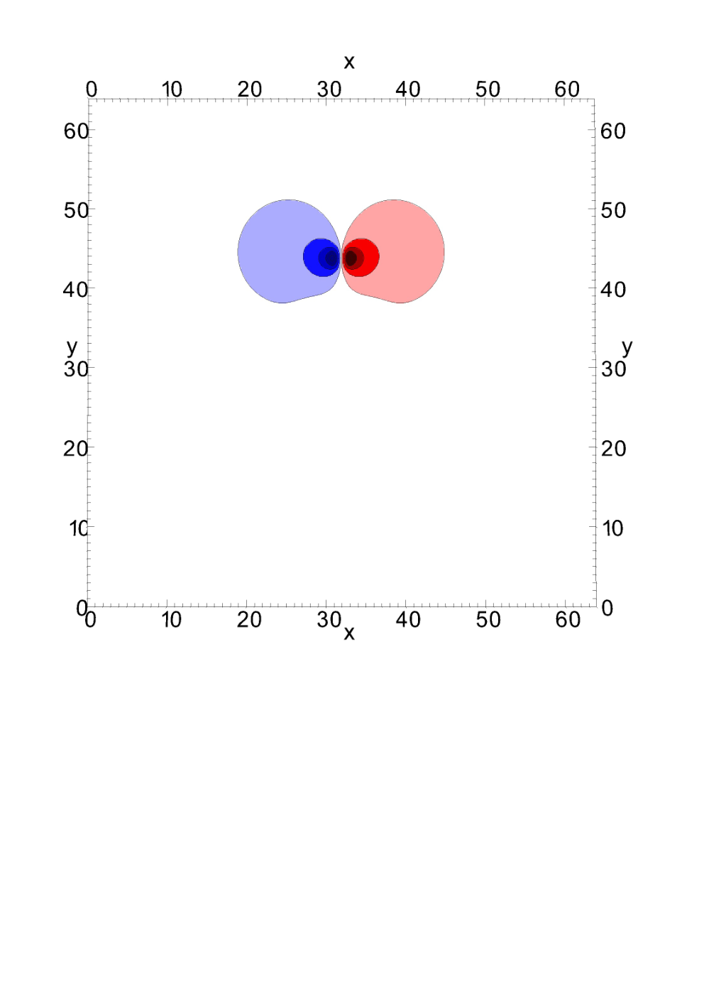
The first electrostatic drift wave test case follows the evolution of Gaussian monopoles. Within the framework of the CHM model, monopoles for various initial amplitudes $A$, correponding to a rotation number $R_{E}=A/{r}_{0}$, exhibit nearly coherent vortex propagation into the diamagnetic (here: $y$) direction for a large $R_{E}\gg 1$, or contrarily, dispersive spreading for small $R_{E}\ll 1$ [24, 37].

In the following test cases, the propagation of initial monopoles with $R_{E}=0.1$ (Fig. 1), $R_{E}=1$ (Fig. 2) and $R_{E}=5$ (Fig. 3) is compared between the LB (first row) and FD (second row) schemes at various times of the computation. The LB algorithm closely resembles the monopole dynamics of the CHM equation posed by the FD scheme, except for a small deviation of the vortex amplitudes at later times (compare Fig. 1 at $t=25$).

Solitary dipole drift vortex solutions or modons are, in contrast to Gaussian monopoles, localized stationary solutions to the CHM equations. For Larichev-Reznik modons, the initial potential perturbation of radial extent ${R}$ is defined as [38, 24]:

with

where $J_{1}$, $J_{2}$ are Bessel functions of the first kind and $K_{1}$, $K_{2}$ are modified Bessel functions of the second kind. The parameter $\beta=\sqrt{1-({u}_{d}/{u}_{*})}$ contains the ratio of the drift velocity ${u}_{d}$ to the dipole velocity ${u}_{*}$. The parameter $\gamma$ is determined by the transcendental equation

Its smallest number defines the ground state of the dipole, and higher order solutions are excited states [39]. The drift modon is stable if the ratio between the typical dipole velocity to the drift velocity fullfills ${u}_{d}/{u}_{*}\geq 1$ whereas dispersive broadening appears for negative ratios. The present computations are restricted to the ground state of stable travelling drift modon with ${u}_{d}/{u}_{*}=2$. Fig. 4 shows the expected propagation of the drift modon into the $+y$ direction. For the LB model (first row) an increased shearing of the drift modon is observed in comparison to the classical FD model (second row) with progressing time. In the LB model the lifetime of the stable travelling drift modon is further enhanced by reducing the drift ratio $\kappa_{n}$.

The initial energy spectrum ${E}_{\delta\phi}({k})\propto{k}^{30}({k}+{k}_{0})^{-60}$ is determined in k-space by a random phase factor and a narrow peak around a wavenumber ${k}_{0}$ [40, 41], which is here is fixed to ${k}_{0}=0.5$. Hence around 32 field modes are initialized into a physical box size of $64\rho_{s}$. The initial amplitude factor of the electrostatic potential field is chosen that both algorithms remain stable during the computation time, whereby the LBM is more restrictive, and $\mathcal{O}(\delta{\phi})=0.5$ is used as an examplary value. This sets the initial values of the total generalized energy and total generalized enstrophy to $\mathcal{E}\approx 0.07$ and $\mathcal{U}\approx 0.7$, which are defined by

The spatial gradients are related to the macroscopic velocity via the lowest order momentum balance equation ${\boldsymbol{e}}_{z}\times{\boldsymbol{u}}=-{\boldsymbol{\nabla}}\delta\phi$. Hence the kinetic energy and the enstrophy are derived by $({\boldsymbol{\nabla}}\delta\phi)^{2}={\boldsymbol{u}}^{2}$ and $({\boldsymbol{\nabla}}^{2}\delta\phi)^{2}=(\partial_{x}u_{y}-\partial_{y}u_{x})^{2}$. The partial derivatives are computed with the help of central differences of second order accuracy. Fig. 5 shows the decaying turbulent potential field. Up to $t\approx 30$ the turbulent field is nearly isotropic. The emerging anisotropy, visible through a pattern of elongated structures into y-direction, gradually increases as the simulation advances. The one-dimensional generalized energy spectra ${E}({k}_{x})$ and ${E}({k}_{y})$ differ by a few orders of magnitude in the high ${k}_{x}$, ${k}_{y}$ range [42], apart from the dumb-bell shaped two-dimensional generalized energy spectrum (cf. [37]). The correlation between the turbulent electrostatic potential fields of the LB and FD scheme decreases as time progresses.

Fig.  shows the corresponding angle-averaged generalized energy spectrum ${E}({k})$ of the nearly isotropic state which is defined as the sum over the energy shell within ${k}\pm\Delta{k}$:

Due to the non-periodicity of the signal in $x$-direction a Blackmann-Harris window [43] has been used on the Fourier transform. As a result the transformed signals do not alter the overall power law coefficient of the $k$-spectrum. The obtained power law coefficients resemble the theoretically [44] and numerically [40, 38, 45] predicted strong turbulence laws

except in the high-$k$ dissipative range, where the power law coefficient steepens to approximately ${k}^{-4}$. The LBM spectrum moreover reveals a weak peak in the very high $k$ range arising from the residual force term contributions of the free-slip boundary condition.

The time evolution of the generalized energy $\mathcal{{E}}$ and enstrophy $\mathcal{U}$ for both algorithms are shown in In Fig.  the time evolution of the generalized energy $\mathcal{{E}}$ and enstrophy $\mathcal{U}$ for both algorithms resembles decay power laws. Due to the different treatment of the viscous dissipation the corresponding decay is slower for the hyperviscvous implementation in the FD scheme. The deviation at $t=0$ of the initial variables is based in the differing resolutions underlying the Fourier transforms of the $k$-spectra, and in the initialization of the dynamical variables itself. The fitted power law coefficients are of same magnitude as the estimates of $\mathcal{U}\propto t^{-0.5}$ and $\mathcal{{E}}\propto t^{-0.05}$ [40].

References

• [1] S. Chen, H. Chen, D. Martnez and W. Matthaeus, Phys. Rev. Lett. 67, 3776–3779 (1991).
• [2] S. Succi, M. Vergassola, R. Benzi, Phys. Rev. A 43, 4521–4524 (1991)
• [3] D.O. Martinez, S. Chen, W.H. Matthaeus, Phys. Plasmas 1, 1850 (1994).
• [4] L. Vahala, D. Wah, G. Vahala, J. Carter, P. Pavlo, Physical Review E 62, 507 (2000).
• [5] W. Schaffenberger, A. Hanselmeier, Phys. Rev. E 66, 046702 (2002)
• [6] P.J. Dellar, Phys. Rev. E, 65, 036309 (2002).
• [7] P.J. Dellar J. Comput. Phys., 190, 351–370 (2003).
• [8] G. Breyiannis, D. Valougeorgis, Phys. Rev. E 69, 065702(R) (2004).
• [9] A. Macnab, G. Vahala, L. Vahala, J. Carter, M. Soe and W. Dorland, Physica A 362, 48 (2006).
• [10] G. Vahala, B. Keating, M. Soe, J. Yepez, L. Vahala, J. Carter et al. Commun. Comput. Phys., 4 (2008), pp. 624–646
• [11] M. Pattison, K. Premnath, N. Morley, M. Abdou, Fusion Eng. Design, 83, 557 (2008).
• [12] J. Statist. Mech. P06003 (2009).
• [13] D. Chatterjee and S. Amiroudine, Phys. Rev. E 81, 066703 (2010)
• [14] P.J. Dellar, Computers & Fluids 46, 201 (2011)
• [15] P.J. Dellar, Journal of Computational Physics 237, 115 (2013).
• [16] P.J. Dellar, J. Comput. Phys. 179, 05 (2002).
• [17] M. Mendoza and J. D. Munoz, Phys. Rev. E 77, 026713 (2008).
• [18] G. Fogaccia, R. Benzi and F. Romanelli, Phys. Rev. E 54 4384, (1996).
• [19] A. Hasegawa, K. Mima, Physical Review Letters 4, 205 (1977).
• [20] J.G. Charney, Geophys. Publ. Oslo 17, 1 (1948).
• [21] A. Kendl, Eur. J. Phys. 29, 911-926 (2008).
• [22] B. D. Scott, Plasma Phys. Control. Fusion 49, S25-41 (2007).
• [23] J. A. Krommes, Annu. Rev. Fluid. Mech. 44, 175-201 (2012).
• [24] W. Horton and A. Hasegawa, Chaos 4, 227 (1994).
• [25] L. H. Zhong, S. D. Feng, S. T. Gao Adv. Atmos. Sci. 22, 349-358 (2005).
• [26] L. Zhong, S. D. Feng, S. T. Gao Advances atmos . Sci 23, 561-578 (2006).
• [27] L. H. Zhong, S. D. Feng, S. T. Gao Chonese J. Geophysics-Chinese Edition 49, 1257-1270 (2006).
• [28] P. J. Dellar, http://www.serc.iisc.ernet.in/∼\simraha/
onGELatticeBoltzmannProblem.pdf (2000), (last accessed on 27.05.2014) .
• [29] P. L. Bhatnagar, E. P. Gross, M. Krook, Phys. Rev. 94, 511-525 (1954).
• [30] R. Salmon, Journal of Marine Research 3, 503-535 (1999)
• [31] L.-S. Luo, Phys. Rev. Lett. 81, 1618 - 1621 (1998)
• [32] P.J. Dellar, Computers & Mathematics with Applications 65, 129 (2013)
• [33] S. Succi, The Lattice Boltzmann Equation for Fluid Dynamics and Beyond. Oxford University Press, 2001.
• [34] V. Naulin and A.H. Nielsen, SIAM J. Sci. Comput. 25, 104 (2003).
• [35] A. Arakawa, Journal of Computational Physics 1, 119 (1966).
• [36] G.E. Karniadakis, S.A. Orszag, and M. Israeli, Journal of Computational Physics 97, 414 (1991).
• [37] V. Naulin, New Journal of Physics 4, 28 (2002).
• [38] C.F. Fontán and A. Varga, Physical Review E 6, 6717 (1995).
• [39] M. Kono and M. Skoric, Nonlinear Physics of Plasmas. Springer, 2010.
• [40] K. Iga and T. Watanabe, Journal of the Meteorological Society of Japan 5, 895 (2003).
• [41] V.D. Larichev and J.C. McWilliams, Phys. Fluids A 5, 938 (1991).
• [42] G. Manfredi, Journal of Plasma Physics 4, 601 (1999).
• [43] F.J. Harris, Proceedings of the IEEE 66, 51 (1978).
• [44] M. Ottaviani and J.A. Krommes, Physical Review Letters 69, 2923 (1992).
• [45] N. Kukharkin, S.A. Orszag and V. Yakhot, Physical Review Letters 13, 2486 (1995).
• [46] P.J. Dellar, Journal of Differential Equations 176, 29 (2001).
• [47] X. He, S. Chen, G. D. Doolen, J. Comput. Phys. 146, 282-300 (1998).
• [48] R. Salmon, J. Marine Res. 57, 847-884 (1999).
• [49] H. Yu, S.S.. Girimaji, L.-S. Luo , J. Comput. Phys. 209, 599-616 (2005).
• [50] M. Tsutahara, M. Okabyashi, T. Kataoka, Computational Fluid Dynamics 2000 (ed N. Satofuka), pp. 529-544 (2001).
• [51] Y. Sone, Boston: Birkhäuser (2002).
• [52] M. Junk, A. Klar, L.S. Luo, J. Comput. Phys. 210, 676-704 (2005).
• [53] M. Junk, W.-A. Yong, Asymptotic Analysis 35, 165-185 (2003).
• [54] T. Inamuro, M. Yoshino, F. Ogino, Phys. Fluids 9, 3535-3542, (1997).
• [55] P. Asinari, Computers and mathematics with Applications 55, 1392-1407 (2008).