Spread of Influence in Weighted Networks under Time and Budget Constraints Thanks: An extended abstract of a preliminary version of this paper appeared in Proceedings of 7th International Conference on Fun with Algorithms (FUN 2014), Lecture Notes in Computer Science Vol. 8496, A. Ferro, F. Luccio, P. Widmayer (Eds.), pp. 100-112, 2014. This work was supported in part by the Slovenian Research Agency (research program P $1$ - $0285$ and research projects J $1$ - $5433$ , J $1$ - $6720$ , and J $1$ - $6743$ ).

Ferdinando Cicalese Affiliation: Department of Computer Science, University of Salerno, Italy, {cicalese,lg,uv}@dia.unisa.it Gennaro Cordasco Affiliation: Department of Psychology, Second University of Naples, Italy, gennaro.cordasco@unina2.it Luisa Gargano Affiliation: Department of Computer Science, University of Salerno, Italy, {cicalese,lg,uv}@dia.unisa.it Martin Milanič Affiliation: University of Primorska, UP IAM and UP FAMNIT, SI 6000 Koper, Slovenia, martin.milanic@upr.si Joseph Peters Affiliation: School of Computing Science, Simon Fraser University, Canada, peters@cs.sfu.ca U. Vaccaro Affiliation: Department of Computer Science, University of Salerno, Italy, {cicalese,lg,uv}@dia.unisa.it

Abstract

Given a network represented by a weighted directed graph $G$ , we consider the problem of finding a bounded cost set of nodes $S$ such that the influence spreading from $S$ in $G$ , within a given time bound, is as large as possible. The dynamic that governs the spread of influence is the following: initially only elements in $S$ are influenced; subsequently at each round, the set of influenced elements is augmented by all nodes in the network that have a sufficiently large number of already influenced neighbors. We prove that the problem is NP-hard, even in simple networks like complete graphs and trees. We also derive a series of positive results. We present exact pseudo-polynomial time algorithms for general trees, that become polynomial time in case the trees are unweighted. This last result improves on previously published results. We also design polynomial time algorithms for general weighted paths and cycles, and for unweighted complete graphs.

Keyword. Social Networks, Spread of Influence, Viral Marketing, Dynamic Monopolies

1 Introduction

1.1 Motivation

Social influence is the process by which individuals adjust their opinions, revise their beliefs, or change their behaviors as a result of interactions with other people. When exposed to the opinions of peers on a given issue, people tend to filter and integrate the information they receive and adapt their own judgements accordingly (see for instance [45]). This human tendency to harmonize their own ideas and customs with the opinions and behaviors of others [4] may occurs for several reasons: a) the basic human need to be liked and accepted by others [6]; b) the belief that others, especially a majority group, have more accurate and trustworthy information than the individual [42]; c) the “direct-benefit” effect, implying that an individual obtains an explicit benefit when he/she aligns his/her behavior with the behavior of others (e.g., [26], Ch. 17). It has not escaped the attention of advertisers¹¹ 1 and politicians too [10, 35, 43, 41] that the natural human tendency to conform can be exploited in viral marketing [34]. Viral marketing refers to the spread of information about products and behaviors, and their adoption by people. According to Lately [22], “the traditional broadcast model of advertising-one-way, one-to-many, read-only is increasingly being superseded by a vision of marketing that wants, and expects, consumers to spread the word themselves”. For what strictly concerns us, the intent of maximizing the spread of viral information across a network naturally suggests many interesting optimization problems. Some of them were first articulated in the seminal papers [32, 33], under various adoption paradigms. The recent monograph [14] contains an excellent description of the area. In the next section, we will explain and motivate our model of information diffusion, state the problem that we are investigating, describe our results, and discuss how they relate to the existing literature.

1.2 The Model

Let $G=(V,E)$ be a directed graph, $c:V\to{\mathbb{N}}=\{1,2,\ldots\}$ be a function assigning costs to vertices and $w:E\to{\mathbb{N}}_{0}=\{0,1,2,\ldots\}$ be a function assigning weights to edges. The value $c(v)$ of each vertex $v\in V$ is a measure of how much it costs to initially convince the member $v$ of the network to endorse a given product/behaviour. The weight of an arc $e=(u,v)\in E$ , denoted either by $w(e)$ or by $w(u,v)$ , represents the amount of influence that node $u$ exercises on node $v$ . Let $t:V\to{\mathbb{N}}_{0}$ be a function assigning thresholds to the vertices of $G$ . For each node $v\in V$ , the threshold value $t(v)$ quantifies how hard it is to influence node $v$ , in the sense that easy-to-influence elements of the network have “low” $t(\cdot)$ values, and hard-to-influence elements have “high” $t(\cdot)$ values [29].

A process of influence diffusion in $G$ , starting at the subset of nodes $S\subseteq V$ (hereafter called target set), is a sequence of vertex subsets

{{\sf Influenced}}[S,0]\subseteq{{\sf Influenced}}[S,1]\subseteq\ldots\subseteq{{\sf Influenced}}[S,\tau]\subseteq\ldots\subseteq V,

where ${{\sf Influenced}}[S,0]=S$ , and such that for all $\tau>0$ ,

{{\sf Influenced}}[S,\tau]={{\sf Influenced}}[S,\tau{-}1]\cup\Big\{u\,:\,\sum_{v\in N^{in}(u)\cap{{\sf Influenced}}[S,\tau{-}1]}\!\!\!\!\!\!\!\!\!\!\!\!w(v,u)\geq t(u)\Big\}.

Here $N^{in}(u)=\{v:(v,u)\in E\}$ denotes the set of incoming neighbors of $u$ , that is, the set of nodes in $G$ having a directed arc towards $u$ . In words, at each round $\tau$ a node $u$ becomes influenced if the sum of the influences exercised on $u$ by $u$ ’s already influenced incoming neighbors meets or exceeds $u$ ’s threshold $t(u)$ . We say that node $u$ is influenced within round $\tau$ if $u\in{{\sf Influenced}}[S,\tau]$ ; $u$ is influenced at round $\tau>0$ if $u\in{{\sf Influenced}}[S,\tau]\setminus{{\sf Influenced}}[S,\tau-1]$ .

The problem that we introduce and study in this paper is defined as follows:

$(\lambda,\beta)$ -Maximally Influencing Set ( $(\lambda,\beta)$ -MIS).
Instance: A directed graph $G=(V,E)$ , node thresholds $t:V\to{\mathbb{N}}_{0}$ , vertex costs $c:V\to{\mathbb{N}}$ , edge influences $w:E\to{\mathbb{N}}_{0}$ , a latency bound $\lambda\in{\mathbb{N}}$ and a budget $\beta\in{\mathbb{N}}$ .
Objective: Find a set $S\subseteq V$ such that $c(S)=\sum_{v\in S}c(v)\leq\beta$ and $|{{\sf Influenced}}[S,\lambda]|$ is as large as possible.

Notice that the assumption that all vertex costs are positive is without loss of generality. Indeed, if $c(v)=0$ for some vertex $v$ in the graph, then we can consider a new graph $G^{\prime}$ obtained from $G$ by eliminating $v$ and by setting

$t^{\prime}(u)=\begin{cases}{\max\{t(u)-w(v,u),0\}}&{\mbox{if $u$ is an out-neighbor of $v$ in $G$}}\\ {t(u)}&{\mbox{otherwise.}}\end{cases}$

The decrease in the threshold of the neighbors of $v$ implies that ${{\sf Influenced}}[S,\tau]$ in $G^{\prime}$ is equal to ${{\sf Influenced}}[S\cup\{v\},\tau]$ in $G$ , for each $S\subseteq V-\{v\}$ and $\tau\geq 1$ ; hence $S$ is an optimal solution for $G^{\prime}$ iff $S\cup\{v\}$ is an optimal solution for the original instance. The above transformation can be carried out for all vertices of zero cost in time $O(|V|+|E|)$ resulting in an equivalent instance in which all vertex costs are positive.

We are also marginally interested in the case in which the influence of each arc and the cost to initially activate each vertex are unitary (i.e., the network is unweighted), and the graph representing the network is symmetric, that is, $(u,v)\in E$ if and only if $(v,u)\in E$ . In this particular scenario, studied in the conference version of this paper [20], the activation process obeys the following simpler rule: ${{\sf Influenced}}[S,0]=S$ , and for all $\tau>0$ ,

{{\sf Influenced}}[S,\tau]={{\sf Influenced}}[S,\tau-1]\cup\Big\{u:\big|N(u)\cap{{\sf Influenced}}[S,\tau-1]\big|\geq t(u)\Big\},\,

and the question is to find a set of vertices $S$ such that $|S|\leq\beta$ and $|{{\sf Influenced}}[S,\lambda]|$ is as large as possible, where $\lambda$ is given as input to the problem.

1.3 Related work

The above algorithmic problems have roots in the general study of the spread of influence in Social Networks (see [14, 26] and references quoted therein). For instance, in the area of viral marketing [23, 24], companies wanting to promote products or behaviors might initially try to target and convince a few individuals who, by word-of-mouth, can trigger a cascade of influence in the network leading to an adoption of the products by a much larger number of individuals.

It is clear that the $(\lambda,\beta)$ -MIS problem represents an abstraction of the viral marketing scenario if one makes the reasonable assumption that an individual decides to adopt the products if a suitable number of his/her friends have adopted the products. Analogously, the $(\lambda,\beta)$ -MIS problem can describe other diffusion problems arising in sociological, economical, and biological networks (again see [26]). Therefore, it comes as no surprise that special cases of our problem (or variants thereof) have recently attracted the attention of the algorithmic community. We shall limit ourselves here to discussing the work that is most directly related to ours, and refer the reader to the monographs [14, 26] for an excellent overview of the area. We just mention that our results also seem to be relevant to other areas, like dynamic monopolies [27, 38] for instance.

The first authors to study problems of the spread of influence in networks from an algorithmic point of view were Kempe et al. [32, 33]. However, they were mostly interested in networks with randomly chosen thresholds. Chen [12] studied the following minimization problem: given an unweighted graph $G$ and fixed thresholds $t(v)$ , for each vertex $v$ in $G$ , find a set of minimum size that eventually influences all (or a fixed fraction of) the nodes of $G$ . He proved a strong inapproximability result that makes unlikely the existence of an algorithm with approximation factor better than $O(2^{\log^{1-\epsilon}|V|})$ . Chen’s result stimulated a series of papers [1, 7, 8, 11, 15, 16, 17, 18, 21, 28, 40, 46] that isolated interesting cases in which the problem (and variants thereof) become tractable.

None of the above quoted papers considered the number of rounds necessary for the spread of influence in the network, the fact that different individuals can exercise different amounts of influence on the same person, or that the cost to initially convince individuals might vary among different members of the network. However, all of these questions correspond to relevant issues. Regarding the first question, it is well known that in viral marketing it is quite important to spread information quickly. Indeed, research in Behavioural Economics shows that humans make decisions mostly on the basis of very recent events, even though they might remember much more [2, 13]. Moreover, the conventional idea of long-living viral spread has been challenged by empirical evidence in several real-life datasets, where it has been found that the processes of influence diffusion do not extend after the first few initial steps [30, 44]. Therefore, it seems reasonable to study processes of information diffusion that reach the desired goals within a fixed time bound. Concerning the second point, it is generally assumed that the influence that a VIP may have on the behaviour of an individual can be much larger than the amount of influence exercised on the same person by a less famous acquaintance, and this phenomenon should be taken into account when designing effective viral marketing campaigns (e.g., see [31, 36]).²² 2 Startups like Klout (http://klout.com) offer a way to quantify the influence of online users of social media. Finally, that different members of the network have different activation costs (see [5], for example) is justified by the reasonable assumption that celebrities or public figures can charge more for their endorsements of products.

The only paper known to us that has studied the spread of influence with constraints on the number of rounds in which the process must be completed (but in unweighted networks and with no costs on vertices) is [19]. How our results are related to [19] will be explained in the next section. Paper [39] studied the problem of finding the smallest set of vertices that can influence a whole graph (again, in unweighted networks and with no costs on vertices), where each vertex has an associated deadline that must be respected by the diffusion process. Finally, we point out that Chen’s inapproximability result [12] still holds if the diffusion process must end in a bounded number of rounds.

1.4 The Results

In light of Chen’s strong inapproximability results [12], we feel motivated to identify special cases for which our general problems become tractable (i.e., tree, cycle, and clique topologies). We also feel that the analyzed networks might approximate some features of real-life networks; for instance, trees emulate hierarchical structure while cliques resemble strongly connected components like communities. Moreover, we believe/hope that our proposed strategies could be useful for the development of novel strategies or heuristics on more elaborate topologies.

Our first result shows that the $(\lambda,\beta)$ -MIS problem cannot be solved in polynomial time on weighted complete graphs unless $P=NP$ . On the other hand, if the graph is complete and unweighted, then a linear time algorithm for the $(\lambda,\beta)$ -MIS problem is quite easy to find.

In Section 3 we turn our attention to trees. We first prove that solving the $(\lambda,\beta)$ -MIS problem on weighted trees is at least as hard as solving general instances of the well-known NP-hard $0-1$ Knapsack problem. Subsequently, we derive pseudo-polynomial time algorithms to solve the $(\lambda,\beta)$ -MIS problem on weighted trees. We point out that the paper [19] provided an algorithmic framework to solve the $(\lambda,\beta)$ -MIS problem (and related ones), in unweighted graphs of bounded clique-width. When instantiated on unweighted trees, the approach of [19] gives algorithms for the $(\lambda,\beta)$ -MIS problem with complexity that is exponential in the parameter $\lambda$ , whereas our algorithm, when instantiated on unweighted trees, has complexity polynomial in all of the relevant parameters (see Corollary 1).

In Section 4, we study the case of weighted paths and cycles and we provide polynomial time algorithms to solve the $(\lambda,\beta)$ -MIS problem on these classes of graphs.

We conclude this discussion by remarking that, in the very special case $\lambda=1$ , thresholds and costs $t(v)=c(v)=1$ for each vertex $v\in V$ , and edge weights $w(e)=1$ for each $e\in E$ , problems of influence diffusion reduce to well-known domination problems in graphs (and variants thereof). In particular, when $\lambda=1$ , $t(v)=c(v)=1$ for each $v\in V$ , and $w(e)=1$ for $e\in E$ , our $(\lambda,\beta)$ -MIS problem reduces to the Maximum Coverage problem considered in [9]. Therefore, our results can also be seen as far-reaching generalizations of [9].

2 Complexity of Computing $(\lambda,\beta)$ -MIS in Complete Graphs

We prove that the $(\lambda,\beta)$ -MIS problem is NP-hard for complete graphs. It was shown in [25] that when $t(v)=d(v)$ for each vertex $v$ , where $d(v)$ denotes the in-degree of $v$ , the problem of finding the minimum size subset $S\subseteq V$ such that ${{\sf Influenced}}[S,\tau]=V$ , for some $\tau\geq 0$ , is equivalent to finding a minimum size vertex cover of the graph. Indeed under the hypothesis that $t(v)=d(v)$ for each $v\in V$ , one has that ${{\sf Influenced}}[S,\tau]={{\sf Influenced}}[S,1]$ for any $S\subseteq V$ and $\tau>0$ ; moreover, ${{\sf Influenced}}[S,1]=V$ if and only if $S$ is a vertex cover for $G$ . This observation was used to prove that, for any constant $k\geq 3$ , the above minimization problem cannot be solved in polynomial time, unless $P=NP$ , in the class of $k$ -regular non-bipartite unweighted graphs. Now, consider the following problem:

$\lambda$ -Minimum Size Subset ( $\lambda$ -MSS).
Instance: A graph $G=(V,E)$ , thresholds $t:V\to{\mathbb{N}}_{0}$ , and a bound $\lambda\in{\mathbb{N}}$ .
Objective: Find a set $S\subseteq V$ of minimum size such that ${{\sf Influenced}}[S,\lambda]=V$ .

Under the assumption that $t(v)=d(v)$ for each $v\in V$ , a minimum size subset $S\subseteq V$ such that ${{\sf Influenced}}[S,\lambda]=V$ (where now $\lambda$ is an input to the problem) would still correspond to a minimum vertex cover of the graph. Hence, The $\lambda$ -MSS problem cannot be solved in polynomial time unless P=NP.

Theorem 1.

The $(\lambda,\beta)$ -MIS problem cannot be solved in polynomial time on weighted complete graphs unless P=NP, even if all vertex costs $c(v)$ are equal to 1.

Proof.

We will prove that if one had a polynomial time algorithm to solve the $(\lambda,\beta)$ -MIS problem on an arbitrary complete weighted graph, then one could also obtain a polynomial time algorithm for the $\lambda$ -MSS problem.

Consider an arbitrary graph $G=(V,E)$ with the thresholds on the nodes given by some function $t:V\to{\mathbb{N}}_{0}$ . Let $n$ denote the size of $V$ . We construct a complete graph $K=(V,F)$ on the same set of vertices $V$ , with weight function on the edges given by

\mbox{for all }(u,v)\in F\quad w(u,v)=\begin{cases}n+1\mbox{ \ \ \ if $\{u,v\}\in E$}\\ 1\mbox{ \ \ \ \ \ \ \ \ \ otherwise,}\end{cases}

and for each node $v\in V$ , the threshold $t^{\prime}(v)$ of $v$ in $K$ equal to

t^{\prime}(v)=(n+1)t(v).

One can easily check that any set of initially influenced nodes $S\subseteq V$ generates the same dynamics of influenced nodes in $G$ and $K$ , that is, for each $\tau\geq 0$ we have that ${{\sf Influenced}}[S,\tau]$ in $G$ is equal to ${{\sf Influenced}}[S,\tau]$ in $K$ . The conclusion of the proof is now clear: if one had a polynomial time algorithm ${\cal A}$ for the $(\lambda,\beta)$ -MIS problem on arbitrary complete weighted graphs, then by using at most $\log|V|$ calls to ${\cal A}$ on the graph $K$ , one could find in polynomial time a minimum size subset $S\subseteq V$ such that ${{\sf Influenced}}[S,\lambda]=V$ in the graph $G$ . This, together with the hardness of the $\lambda$ -MSS problem, completes the proof. ∎

We now turn our attention to positive results, restricting our attention to complete graphs in which all edge weights are equal. Without loss of generality, we can assume that all edge weights are equal to 1. Since complete graphs are of clique-width at most $2$ , results from [19] imply that the $(\lambda,\beta)$ -MIS problem is solvable in polynomial time on such a class of graphs, if $\lambda$ is constant. Indeed, one can see that the $(\lambda,\beta)$ -MIS can be solved in linear time, independently of the value of $\lambda$ , by using ideas from [37].

If the network is a complete graph, then for any subset of vertices $S$ and any round $\tau\geq 1$ , it holds that

{{\sf Influenced}}[S,\tau]={{\sf Influenced}}[S,\tau-1]\cup\{v\,:\,t(v)\leq|{{\sf Influenced}}[S,\tau-1]|\}.

Since ${{\sf Influenced}}[S,\tau-1]\subseteq{{\sf Influenced}}[S,\tau],$ we have

{{\sf Influenced}}[S,\tau]=S\cup\{v\,:\,t(v)\leq|{{\sf Influenced}}[S,\tau-1]|\}.

(1)

From (1), and by using a standard exchange argument, one realizes that a set $S$ with largest influence is the one containing the nodes with highest thresholds. Since it is customary in the case of unweighted graphs to make the reasonable assumption that $t(v)\in\{0,1,\ldots,n\}$ , the selection of the $\beta$ nodes with highest threshold can be done in linear time. Summarizing, we have the following result.

Theorem 2.

There exists an optimal solution $S$ to the $(\lambda,\beta)$ -MIS problem on a complete unweighted graph $G=(V,E)$ that consists of the $\beta$ nodes of $V$ with highest thresholds, and this solution can be computed in linear time.

3 Complexity of Computing $(\lambda,\beta)$ -MIS in Weighted Trees

We first show that the $(\lambda,\beta)$ -MIS problem on weighted trees is at least as hard as the well-known $0-1$ Knapsack problem, which is defined as follows:

$0-1$ Knapsack.
Instance: $n$ items, $o_{1},o_{2},\ldots,o_{n}$ , where each $o_{i}$ has a profit $p_{i}$ and weight $w_{i},$ a knapsack capacity $W,$ and a profit bound $P$ .
Question: Does there exist a subset of items $\{o_{i_{1}},o_{i_{2}},\ldots,o_{i_{k}}\}$ , such that $\sum_{j=1}^{k}w_{i_{j}}\leq W$ and $\sum_{j=1}^{k}p_{i_{j}}\geq P$ ?

Refer to caption — Figure 1: The weighted tree $T$ .

Theorem 3.

The $(\lambda,\beta)$ -MIS problem cannot be solved in polynomial time on weighted star graphs unless P=NP.

Proof.

Our reduction will be from the $0-1$ Knapsack problem. Starting from an instance of the $0-1$ Knapsack problem, we build a weighted tree $T=(V,E)$ as depicted in Figure 1. The tree $T$ consists of $n+1$ nodes, one node $v_{i}$ for each item $o_{i}$ plus an additional node $v_{n+1}$ . For each $i=1,2,\ldots,n,$ the node $v_{i}$ has a directed edge to node $v_{n+1}$ with weight $w(v_{i},v_{n+1})=p_{i}$ . For each $i=1,2,\ldots,n,$ the threshold of node $v_{i}$ is $t(v_{i})=0$ , and the cost of node $v_{i}$ is $c(v_{i})=w_{i}$ , while $t(v_{n+1})=P$ and $c(v_{n+1})=W+1$ . It is easy to see that $T$ has a target set $S\subseteq V$ of total cost at most $W$ such that ${{\sf Influenced}}[S,1]=V$ if and only if the instance of the $0-1$ Knapsack problem has a Yes answer, from which the theorem easily follows.

Let $S=\{v_{i_{1}},v_{i_{2}},\ldots,v_{i_{k}}\}\subseteq V$ be a target set for $T$ such that $\sum_{j=1}^{k}c(v_{i_{j}})\leq W$ and ${{\sf Influenced}}[S,1]=V.$ Since $c(v_{n+1})=W+1$ we have that $v_{n+1}\notin S$ . The inequality $\sum_{j=1}^{k}c(v_{i_{j}})\leq W$ implies that $\sum_{j=1}^{k}w_{i_{j}}\leq W$ . The hypothesis that ${{\sf Influenced}}[S,1]=V$ implies that $v_{n+1}\in{{\sf Influenced}}[S,1]$ , that is, $\sum_{j=1}^{k}w(v_{i_{j}},v_{n+1})\geq t(v_{n+1})=P$ . Consequently $\sum_{j=1}^{k}p_{i_{j}}\geq P$ .

Conversely, let $K=\{o_{i_{1}},o_{i_{2}},\ldots,o_{i_{k}}\}$ be a subset of items such that $\sum_{j=1}^{k}w_{i_{j}}\leq W$ and $\sum_{j=1}^{k}p_{i_{j}}\geq P$ . Let $S=\{v_{i_{1}},\ldots v_{i_{k}}\}$ . We have that $c(S)\leq W$ . Since for each $i=1,2,\ldots,n,$ it holds that $t(v_{i})=0$ , we also have $\{v_{1},v_{2},\ldots,v_{n}\}\subseteq{{\sf Influenced}}[S,1]$ . Moreover, the hypothesis that $\sum_{j=1}^{k}p_{i_{j}}\geq P$ directly implies that $\sum_{j=1}^{k}w(v_{i_{j}},v_{n+1})=\sum_{j=1}^{k}p_{i_{j}}\geq P$ , consequently the nodes in $S$ are able to influence the node $v_{n+1}$ in one step, that is, ${{\sf Influenced}}[S,1]=V$ . ∎

In the rest of this section we derive a pseudo-polynomial time algorithm for the $(\lambda,\beta)$ -MIS problem on weighted trees. Let $T=(V,E)$ be a tree having $n$ nodes. Let us denote by $\Delta$ the maximum indegree of $T$ , that is, the quantity

\Delta=\max_{v\in V}|\{u:(u,v)\in E\}|

and by $W$ the quantity

W=\max_{v\in V}\left\{\sum_{u\in N^{in}(v)}w(u,v)\right\}.

In the following, we will assume that $T$ is rooted at some node $r$ . For any node $v$ in this rooted tree, we denote the subtree rooted at $v$ by $T(v)$ , the set of children of $v$ by $C(v)$ , and the parent of $v$ in $T$ , for $v\neq r,$ by $p(v)$ . We will develop a dynamic programming algorithm that will prove the following theorem.

Theorem 4.

The $(\lambda,\beta)$ -MIS problem can be solved in time $O(\Delta\,\lambda^{2}W\beta^{3})$ on a weighted tree with maximum in-degree $\Delta$ and total edge weight $W$ .

The rest of this section is devoted to the design and analysis of the algorithm that proves Theorem 4. The algorithm traverses the input tree $T$ bottom up, in such a way that each node is considered after all of its children have been processed. The basic idea is that the nodes in one subtree of a given node $v$ cannot influence nodes in another subtree without passing through $v$ . Moreover, considering a node $v$ and one of its children $u$ , there are three possibilities: $v$ influences $u$ (in this case $v$ must be influenced before $u$ ); $u$ influences $v$ (in this case $u$ must be influenced before $v$ ); they do not influence each other (the nodes in $T(u)$ cannot influence any other node in $T\setminus T(u)$ ). Two particular cases will be considered:

•

$v$ belongs to the initial target set $S$ . In this case all of the children of $v$ can exploit the influence of $v$ starting in round $1$ ;
•

$v\notin{{\sf Influenced}}[S,\lambda]$ .

In both of these particular cases, the nodes that belong to different subtrees of $v$ cannot influence each other. In light of the above observations, for each node $v$ , the algorithm solves all possible $(\tau,\beta)$ -MIS problems on $T(v)$ for all possible values of $\tau\leq\lambda$ and $\beta\leq b$ . Moreover, for some of these values, we will consider not only the original threshold $t(v)$ of $v$ , but also the decreased value

t^{\prime}(v)=\left\{\begin{array}[]{ll}\max\{t(v)-w(p(v),v),0\}&\hbox{if $v\neq r$}\\ t(v)&\hbox{if $v=r$}\end{array}\right.

(2)

which we will refer to as the residual threshold. The original threshold is used when the nodes in the subtree $T(v)$ are not influenced by $p(v)$ and consequently by any other nodes in $T\setminus T(v)$ . The residual threshold is used when $p(v)$ influences $v$ . In this case the strategy must guarantee that $p(v)$ will be influenced before $v$ .

In the following, we assume without loss of generality that

0\leq t(u)\leq W(u)+1,

where $W(u)=\sum_{v\in N^{in}(u)}w(v,u),$ holds for all nodes $u\in V$ (otherwise, we can set $t(u)=W(u)+1$ for every node $u$ with threshold exceeding $W(u)+1$ without changing the problem).

Definition 1.

For each node $v\in V$ , integers $b=0,1,\dots,\beta$ , $t\in\{t^{\prime}(v),t(v)\}$ , and $\tau\in\{0,1,\ldots,\lambda,\infty\}$ , let us denote by $MIS[v,b,\tau,t]$ the maximum number of nodes that can be influenced in $T(v)$ , in at most $\lambda$ rounds, starting with a target set $S\subseteq V(T(v))$ , assuming that

•

the target set is of total cost at most $b$ , that is, $c(S)\leq b$ ;
•

the threshold of $v$ is $t$ , and for every $u\in V(T(v))\setminus\{v\}$ , the threshold of $u$ is $t(u)$ ;

•

the parameter $\tau$ is such that

		$\displaystyle 1)\mbox{ if $\tau=0$ then $v$ must belong to the target set,}$		(3)
		$\displaystyle 2)\mbox{ if $1\leq\tau\leq\lambda$ then $v$ is not in the target set and the influence of $v$'s }$
		children at round $\tau-1$ is sufficiently large to activate $v$ at round $\tau$ ,
		that is $\sum_{u\in C(v)\cap{{\sf Influenced}}[S,\tau-1]}w(u,v)\geq t$ ;		(4)
		$\displaystyle 3)\mbox{ if $\tau=\infty$ then $v$ is not influenced within round $\lambda$.}$		(5)

We define $MIS[v,b,\tau,t]=-\infty$ when the above problem is infeasible. For instance, if $\tau=0$ and $b<c(v)$ we have $MIS[v,b,0,t]=-\infty$ .

Denote by $S(v,b,\tau,t)$ any target set $S\subseteq V(T(v))$ attaining the value $MIS[v,b,\tau,t]$ (in case of feasible instances).

We notice that in the above definition, if $1\leq\tau\leq\lambda$ , then the assumption that $v$ has threshold $t$ implies that $v$ is influenced by round $\tau$ and it is able to start influencing its neighbors no later than at round $\tau+1$ .³³ 3 Notice that this does not exclude the case that $v$ becomes an influenced node at some round before $\tau^{\prime}<\tau$ . The value $\tau=\infty$ means that $v$ could be either influenced after round $\lambda$ or not influenced at all.

Remark 1.

It is worthwhile mentioning that $MIS[v,b,\tau,t]$ is monotonically non-decreasing in $b$ and non-increasing in $t$ . However, $MIS[v,b,\tau,t]$ is not necessarily monotone in $\tau$ .

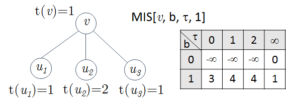
Indeed, partition the set $C(v)$ into two sets: $C^{\prime}(v)$ , which contains the $t$ children that influence $v$ , and $C^{\prime\prime}(v)$ , which contains the remaining $|C(v)|-t$ children that may be influenced by $v$ . A small value of $\tau$ may require a higher budget on subtrees rooted at a node $u\in C^{\prime}(v)$ , and may save some budget on the remaining subtrees; the opposite happens for a large value of $\tau$ . An example is depicted in Figure 2. In the example, all of the node costs $c(\cdot)$ and edge weights $w(\cdot)$ are equal to $1$ . The table reports the value of $MIS[v,b,\tau,1]$ for each $b\in\{0,1\}$ and $\tau\in\{0,1,2,\infty\}$ .

The maximum number of nodes in $T$ that can be influenced within round $\lambda$ with any (initial) target set of cost at most $\beta$ can then be obtained by computing

\max_{\tau\in\{0,1,\ldots,\lambda,\infty\}}\ MIS[r,\beta,\tau,t(r)].

(6)

We compute this quantity in Lemma 1 by decomposing

\max_{\tau\in\{0,1,\ldots,\lambda,\infty\}}\ MIS[v,b,\tau,t],

for each $v\in V,$ each $b=0,1,\ldots,\beta$ , and each $t\in\{t^{\prime}(v),t(v)\}$ , into a maximum of three other values which are successively and separately computed in Lemmata 2–6.

We proceed in a bottom-up fashion on the tree, so that the computation of the various values $MIS[v,b,\tau,t]$ for a node $v$ is done after all of the values for $v$ ’s children are known.

For each leaf node $\ell$ we have

MIS[\ell,b,\tau,t]=\begin{cases}1&\mbox{ if }(\tau=0\mbox{ AND }b\geq c(\ell))\mbox{ OR }(t=0\mbox{ AND }1\leq\tau\leq\lambda)\\ 0&\mbox{ if }\tau=\infty\\ -\infty&\mbox{otherwise.}\end{cases}

(7)

Indeed, a leaf $\ell$ gets influenced, in the one-node subtree $T(\ell)$ , only when either $\ell$ belongs to the target set ( $\tau=0$ ) and the budget is sufficiently large ( $b\geq c(\ell)$ ) or the threshold is zero (either $t=t(\ell)=0$ or $t=t^{\prime}(\ell)=0$ ) independently of the number of rounds.

For any internal node $v$ , we show how to compute each value $MIS[v,b,\tau,t]$ in time $O(d(v)W(v)\lambda\beta^{2})$ , where $d(v)$ denotes the in-degree of $v$ .

It will be convenient to analyze the behavior of $MIS[v,b,\tau,t]$ by dividing the possible values of $\tau$ into three cases, according to whether $\tau=0$ , $\tau\in\{1,\dots,\lambda\}$ , or $\tau=\infty.$

To this aim, we will now define three functions, which will be useful for the analysis and the computation of $MIS[\cdot,\cdot,\cdot,\cdot]$ .

In the following we shall also assume that an order has been fixed on the children of any node $v$ , that is, if $v$ has $d$ children we denote them as $v_{1},v_{2},\dots,v_{d},$ according to the fixed order. Also, we define $F(v,i)$ to be the forest consisting of the subtrees rooted at the first $i$ children of $v,$ i.e., $F(v,i)=T(v_{1})\cup\cdots\cup T(v_{i}).$ We will also use $F(v,i)$ to denote the set of vertices it includes.

Definition 2.

Let $v$ be a vertex with $d$ children. For $i=1,\ldots,d$ and $j=0,\ldots,\beta-1$ , let $A_{v}[i,j]$ be the maximum number of nodes that can be influenced, within $\lambda$ rounds, in $F(v,i)$ by an influence diffusion process in $T(v)$ , assuming that the target set contains $v$ and a subset of nodes of $F(v,i)$ of total cost at most $j$ .

Proposition 1.

For each vertex $v$ with $d$ children, each $b=0,1,\ldots,\beta$ , and each $t\in\{t(v),t^{\prime}(v)\}$ , it holds that

MIS[v,b,0,t]=\begin{cases}1+A_{v}[d,b-c(v)]&\mbox{ if }b\geq c(v)\\ -\infty&otherwise.\end{cases}

(8)

Proof.

By Definition 1, if $b<c(v)$ then the statement is trivially true. Otherwise, the statement directly follows from Definitions 1 and 2. In fact we have

$\displaystyle MIS[v,b,0,t]$	$\displaystyle=$	$\displaystyle\max_{\begin{subarray}{c}S\subseteq T(v)\\ v\in S,c(S)\leq b\end{subarray}}\|{{\sf Influenced}}[S,\lambda]\cap T(v)\|$
	$\displaystyle=$	$\displaystyle 1+\max_{\begin{subarray}{c}v\in S\subseteq T(v)\\ c(S\cap F(v,d))\leq b-c(v)\end{subarray}}\|{{\sf Influenced}}[S,\lambda]\cap F(v,d)\|\;$
		$\displaystyle\qquad\qquad\qquad\qquad\qquad\quad(\mbox{since }v\in S\subseteq{{\sf Influenced}}[S,\lambda])$
	$\displaystyle=$	$\displaystyle 1+A_{v}[d,b-c(v)]\,\quad\qquad(\mbox{by definition of }A_{v}[\cdot,\cdot]).$

∎

Definition 3.

Let $v$ be a vertex with $d$ children and let $\tau=1,\dots,\lambda.$ For $i=1,\ldots,d$ , $j=0,1,\ldots,\beta$ , and $k=0,1,\dots,t(v),$ we define $B_{v,\tau}[i,j,k]$ (resp. $B_{v,\tau}[\{i\},j,k]$ ) to be the maximum number of nodes that can be influenced, within $\lambda$ rounds, by any influence diffusion process in $F(v,i)$ (resp. $T(v_{i})$ ) assuming that

•

the target set $S$ is contained in $F(v,i)$ (resp. $T(v_{i})$ ) and is of cost at most $j$ ,
•

at time $\tau+1$ the threshold of $v_{\ell}$ becomes $t^{\prime}(v_{\ell}),$ for each $\ell=1,\dots,i$ , and
•

$\displaystyle{\sum_{\begin{subarray}{c}u\in\{v_{1},\dots,v_{i}\}\\ u\in{{\sf Influenced}}[S,\tau-1]\end{subarray}}w(u,v)\geq k}$ .

We also define $B_{v,\tau}[i,j,k]=-\infty$ (resp. $B_{v,\tau}[\{i\},j,k]=-\infty$ ) when the above constraints are not satisfiable.

Hence, $B_{v,\tau}[\{i\},j,k]$ is the same as $B_{v,\tau}[i,j,k]$ but computed on the subtree $T(v_{i})$ instead of the forest $F(v,i)$ . Since $F(v,1)=T(v_{1})$ , as a particular case, we have $B_{v,\tau}[1,j,k]=B_{v,\tau}[\{1\},j,k].$

Proposition 2.

For each vertex $v$ with $d$ children, each $b=0,1,\ldots,\beta$ , each $\tau=1,\dots,\lambda,$ and each $t\in\{t(v),t^{\prime}(v)\}$ , it holds that

MIS[v,b,\tau,t]\geq 1+B_{v,\tau}[d,b,t].

(9)

Proof.

Let $S$ be a target set achieving $B_{v,\tau}[d,b,t].$ Then $B_{v,\tau}[d,b,t]$ is the number of influenced nodes within $\lambda$ rounds, when the influence diffusion process is run on $F(v,d)$ starting with $S$ . We recall that, by definition, the following conditions are satisfied.

1.

$S\subseteq F(v,d)$ and $c(S)\leq b$
2.

$\displaystyle{\sum_{\begin{subarray}{c}i=1,\dots,d\\ v_{i}\in{{\sf Influenced}}[S,\tau-1]\end{subarray}}w(v_{i},v)\geq t}$
3.

from round $\tau+1$ the threshold of $v_{\ell}$ is decreased to $t^{\prime}(v_{\ell}),$ for each $\ell=1,\dots,d$

Now if we use the same target set $S$ in the subtree $T(v)$ with the original thresholds, except for $t(v)=t$ we get that $v$ is influenced within time $\tau$ as a consequence of condition 2. We observe that $MIS[v,b,\tau,t]$ is the largest possible size achievable for ${{\sf Influenced}}[S,\lambda]$ under condition 1, and the condition that $v$ is influenced within round $\tau$ . Finally, considering that the set of influenced vertices contains $v$ , we have (9). ∎

Definition 4.

Let $v$ be a vertex with $d$ children. For $i=1,\ldots,d$ and $j=0,\ldots,\beta$ , let $C_{v}[i,j]$ be the maximum number of nodes that can be influenced, within $\lambda$ rounds, by an influence diffusion process in $F(v,i)$ assuming that the target set $S\subseteq F(v,i)$ is of cost at most $j$ .

Proposition 3.

For each vertex $v$ with $d$ children, each $b=0,1,\ldots,\beta$ , and each $t\in\{t(v),t^{\prime}(v)\}$ such that there exists a target set $S\subseteq F(v,d)$ with $c(S)\leq b$ and $v\not\in{{\sf Influenced}}[S,\lambda]$ , it holds that

MIS[v,b,\infty,t]=C_{v}[d,b].

(10)

Proof.

We have

$\displaystyle MIS[v,b,\infty,t]$	$\displaystyle=$	$\displaystyle\max_{\begin{subarray}{c}S\subseteq F(v,d)\\ c(S)\leq b\\ v\not\in{{\sf Influenced}}[S,\lambda]\end{subarray}}\|{{\sf Influenced}}[S,\lambda]\|$	(11)
	$\displaystyle=$	$\displaystyle\max_{\begin{subarray}{c}S\subseteq F(v,d)\\ c(S)\leq b\\ v\not\in{{\sf Influenced}}[S,\lambda]\end{subarray}}\sum_{i=1}^{d}\|{{\sf Influenced}}[S,\lambda]\cap T(v_{i})\|$	(12)
	$\displaystyle=$	$\displaystyle\max_{\begin{subarray}{c}S\subseteq F(v,d)\\ c(S)\leq b\end{subarray}}\sum_{i=1}^{d}\|{{\sf Influenced}}[S\cap T(v_{i}),\lambda]\cap T(v_{i})\|$	(13)
	$\displaystyle=$	$\displaystyle C_{v}[d,b],$	(14)

where (12) follows from (11) because, assuming $v$ is not influenced, there is no influence spreading between $T(v_{i})$ and $T(v_{j})$ for any $1\leq i,j\leq d$ with $i\neq j$ ; (13) follows from (12) because if there is no influence spreading between two different subtrees of $F(v,d)$ , then the set of influenced nodes can be computed independently in each subtree; finally (14) follows from (13) by the definition of $C_{v}[d,b].$ ∎

Lemma 1.

For each vertex $v$ with $d$ children, each $b\in\{0,1,\ldots,\beta\}$ , and each $t\in\{t(v),t^{\prime}(v)\}$ , it holds that

\max_{\tau\in\{0,1,\ldots,\lambda,\infty\}}MIS[v,b,\tau,t]=\max\left\{1+A_{v}[d,b-c(v)],1+\max_{1\leq\tau_{1}\leq\lambda}B_{v,\tau_{1}}[d,b,t],C_{v}[d,b]\right\}.

(15)

Moreover, the knowledge of quantities $A_{v}[d,b-c(v)]$ , $B_{v,\tau}[d,b,t]$ , and $C_{v}[d,b]$ also allows the computation of $MIS[v,b,\tau,t]$ for each value of $\tau\in\{0,1\ldots,\lambda,\infty\}$ .

Proof.

For notational convenience, let $M$ denote the right hand side of (15). First, suppose that there exists a target set $S\subseteq F(v,d)$ with $c(S)\leq b$ such that $v\not\in{{\sf Influenced}}[S,\lambda]$ . Then, by Propositions 1, 2, and 3, we have

\max_{\tau\in\{0,1,\ldots,\lambda,\infty\}}MIS[v,b,\tau,t]\geq M.

Now, suppose that for every target set $S\subseteq F(v,d)$ with $c(S)\leq b$ we have $v\in{{\sf Influenced}}[S,\lambda]$ . We claim that in this case we have

C_{v}[d,b]\leq B_{v,1}[d,b,t]+1\,.

Indeed, let $S$ be a target set achieving $C_{v}[d,b]$ . Running the influence diffusion process on $F(v,d)$ with $S$ is equivalent to running the process on $T(v)$ and ignoring the influence of $v$ on its children (which can be modelled by setting $w(v,v_{i})=0$ for each $i=1,\dots,d$ ). It can be seen that, given the target set $S$ , increasing the weights on some edges cannot decrease the number of nodes in $F(v,d)$ influenced within $\lambda$ rounds. This implies that $C_{v}[d,b]$ is not greater than the number of nodes in $F(v,d)$ influenced within $\lambda$ rounds when the influence diffusion process is run from $S$ in the tree $T(v)$ with the original threshold, which, in turn, does not exceed $B_{v,1}[d,b,t]+1$ .

Summarizing the above two cases, we see that in any case we have

\max_{\tau\in\{0,1,\ldots,\lambda,\infty\}}MIS[v,b,\tau,t]\geq M.

(16)

To see that the converse inequality

\max_{\tau\in\{0,1,\ldots,\lambda,\infty\}}MIS[v,b,\tau,t]\leq M

(17)

also holds, let $\tau^{*}\in{\rm argmax}_{\tau\in\{0,1,\ldots,\lambda,\infty\}}MIS[v,b,\tau,t].$

If $\tau^{*}=0$ , we have $1+A_{v}[d,b-c(v)]=MIS[v,b,\tau^{*},t]$ by Proposition 1. Analogously, if $\tau^{*}=\infty$ then $v\not\in{{\sf Influenced}}[S,\lambda]$ for the target set $S$ achieving $MIS[v,b,\tau^{*},t]$ by Proposition 3. Then, by Definition 1, we have $C_{v}[d,b]=MIS[v,b,\tau^{*},t].$ Hence, in both of the above cases, the desired inequality (17) also holds a fortiori.

Let us now assume that $\tau^{*}\in\{1,\dots,\lambda\}.$ Let $S\subseteq F(v,d)$ be a target set of cost at most $b$ which achieves $MIS[v,b,\tau^{*},t].$ Let $\tilde{\tau}\leq\tau^{*}$ be the minimum positive integer such that $v\in{{\sf Influenced}}[S,\tilde{\tau}].$ Therefore, no influence is spread from $v$ towards the subtrees of $F(v,d)$ before round $\tilde{\tau}.$ Let $S_{i}=S\cap T(v_{i}).$ The previous observation implies that ${{\sf Influenced}}[S,\tau]\cap T(v_{i})={{\sf Influenced}}[S\cap T(v_{i}),\tau]$ for each $\tau\leq\tilde{\tau},$ i.e., the spread of influence within $T(v_{i})$ until round $\tau$ is only determined by the set $S_{i}.$ From $\tilde{\tau}$ on, in $T(v_{i})$ the fact that $v$ is influenced is equivalent to saying that the threshold of $v_{i}$ has been decreased to $t^{\prime}(v_{i}).$

Formally, this means that

\left|\bigcup_{i}\left({{\sf Influenced}}[S,\lambda]\cap T(v_{i})\right)\right|\leq B_{v,\tilde{\tau}}[d,b,t]

hence we have

$\displaystyle\max_{\tau\in\{1,\ldots,\lambda\}}MIS[v,b,\tau,t]$	$\displaystyle=$	$\displaystyle MIS[v,b,\tau^{*},t]$	(18)
	$\displaystyle=$	$\displaystyle 1+\left\|\bigcup_{i}\left({{\sf Influenced}}[S,\lambda]\cap T(v_{i})\right)\right\|$
	$\displaystyle\leq$	$\displaystyle 1+B_{v,\tilde{\tau}}[d,b,t]$
	$\displaystyle\leq$	$\displaystyle 1+\max_{\tau\in\{1,\ldots,\lambda\}}B_{v,\tau}[d,b,t].$

This concludes the proof of (17) that, together with (16), yields the desired result, i.e., formula (15).

Notice that the above reasoning proves a slightly more general fact, that is, the inequality

\max_{\tau^{\prime}\in\{1,\ldots,\tau\}}MIS[v,b,\tau^{\prime},t]\leq 1+\max_{\tau^{\prime}\in\{1,\ldots,\tau\}}B_{v,\tau^{\prime}}[d,b,t]

(19)

for any $\tau=1,2,\ldots,\lambda$ . Formula (19), together with Proposition 2, allows us to conclude that

\max_{\tau^{\prime}\in\{1,\ldots,\tau\}}MIS[v,b,\tau^{\prime},t]=1+\max_{\tau^{\prime}\in\{1,\ldots,\tau\}}B_{v,\tau^{\prime}}[d,b,t]

(20)

for any $\tau=1,2,\ldots,\lambda.$

Moreover, for each $\tau=1,2,\ldots,\lambda-1$ we also have $MIS[v,b,\tau,t]\leq MIS[v,b,\tau+1,t]$ . Therefore by comparing $\max_{\tau^{\prime}\in\{1,...,\tau\}}MIS[v,b,\tau^{\prime},t]$ and $\max_{\tau^{\prime}\in\{1,...,\tau+1\}}MIS[v,b,\tau^{\prime},t]$ , we are also able to compute $MIS[v,b,\tau,t]$ for each value of $\tau=1,2,\ldots,\lambda.$ Recalling that, for $\tau=0$ and $\tau=\infty$ , the value of $MIS[v,b,\tau,t]$ is easily determined using Propositions 1 and 3, respectively, we have that the knowledge of quantities $A_{v}[d,b-c(v)]$ , $C_{v}[d,b]$ , and $B_{v,\tau_{1}}[d,b,t]$ for each $\tau_{1}=1,\ldots,\lambda$ also allows the computation of $MIS[v,b,\tau,t]$ for each value of $\tau\in\{0,1\ldots,\lambda,\infty\}$ . ∎

Lemma 2.

For each vertex $v$ , for each $b=0,1,\ldots,\beta$ , and for each $t\in\{t(v),t^{\prime}(v)\}$ , the quantity $MIS[v,b,0,t]$ can be computed in time $O(d\lambda b^{2}),$ where $d$ is the number of children of $v$ .

Proof.

If $b<c(v)$ then the problem is infeasible and $MIS[v,b,0,t]=-\infty$ . Otherwise, by Proposition 1, it is enough to show that we can compute $A_{v}[d,b-c(v)]$ in the claimed bound. This will be a consequence of the following recursive characterization of $A_{v}[i,j]$ , for each $i=1,2,\ldots,d$ and $j=0,1,\ldots,b-c(v)$ .

For $i=1$ , we have

A_{v}[1,j]=\max_{\tau_{1},t_{1}}\{MIS[v_{1},j,\tau_{1},t_{1}]\},

(21)

where

1.~\tau_{1}\in\{0,\ldots,\lambda,\infty\}\qquad 2.~t_{1}\in\{t(v_{1}),t^{\prime}(v_{1})\}\qquad 3.~{\rm{if}}~t_{1}=t^{\prime}(v_{1}){\rm{~then}}~\tau_{1}\geq 1.

To see that the left hand side of (21) is at least as large as the right hand side we observe that

	$\displaystyle A_{v}[1,j]$	$\displaystyle=$	$\displaystyle\max_{\tau_{1}\in\{0,1,\dots,\lambda,\infty\}}MIS[v_{1},j,\tau_{1},t^{\prime}(v_{1})]$
		$\displaystyle\geq$	$\displaystyle\max\{MIS[v_{1},j,0,t(v_{1})],\max_{\tau_{1}\in\{1,\dots,\lambda,\infty\}}MIS[v_{1},j,\tau_{1},t^{\prime}(v_{1})]\}$

and the last expression is exactly the right hand side of (21).

For the inequality in the other direction, let $S\subseteq T(v)$ be a target set (of cost at most $j$ ) achieving $A_{v}[1,j].$ If $v_{1}\in S$ then the node $v$ does not have any effect on the nodes influenced in $T(v_{1}).$ Hence we have

A_{v}[1,j]=|{{\sf Influenced}}[S,\lambda]\cap T(v_{1})|\leq MIS[v_{1},j,0,t(v_{1})|.

(22)

If $v_{1}\not\in S$ then let $\tau^{*}\in\{1,\dots,\lambda,\infty\}$ be the minimum positive integer such that $v_{1}$ is influenced at time $\tau^{*}$ because of $S$ ; $v_{1}\not\in{{\sf Influenced}}[S,\lambda]$ then $\tau^{*}=\infty.$ Then, since in the definition of $A_{v}[1,j]$ we assume that $v$ is influenced, or equivalently that the threshold of $v_{1}$ is reduced to $t^{\prime}(v_{1})$ , we have that

A_{v}[1,j]=|{{\sf Influenced}}[S,\lambda]\cap T(v_{1})|\leq MIS[v_{1},j,\tau^{*},t^{\prime}(v_{1})],

(23)

where the last inequality follows by observing that, in the middle expression, the role of $v$ is only to reduce the threshold of $v_{1}$ to $t^{\prime}(v_{1}).$

The last expressions in both (22)-(23) contribute to the $\max$ on the right hand side of (21), hence this is also an upper bound for $A_{v}[1,j]$ .

For $i>1$ , we will show that

A_{v}[i,j]=\max_{0\leq a\leq j}\left\{A_{v}[i-1,a]+\max_{\tau_{i},t_{i}}\{MIS[v_{i},j-a,\tau_{i},t_{i}]\}\right\}

(24)

where

1.~\tau_{1}\in\{0,\ldots,\lambda,\infty\}\qquad 2.~t_{1}\in\{t(v_{1}),t^{\prime}(v_{1})\}\qquad 3.~{\rm{if}}~t_{i}=t^{\prime}(v_{i}){\rm{~then}}~\tau_{i}\geq 1.

This means that we can compute the quantity $A_{v}[i,j]$ by considering all possible ways of partitioning the budget $j$ into two values $a$ and $j-a$ , recursively solving a subproblem on $F(v,i-1)$ with budget $a$ and a subproblem on $T(v_{i})$ with budget $j-a$ , and then combining the solutions.

In order to prove (24) we have

$\displaystyle A_{v}[i,j]$	$\displaystyle=$	$\displaystyle\max_{\begin{subarray}{c}S\subseteq F(v,i)\\ c(S)\leq j\end{subarray}}\|{{\sf Influenced}}[S\cup\{v\},\lambda]\cap F(v,i)\|$	(25)
	$\displaystyle=$	$\displaystyle\max_{\begin{subarray}{c}S\subseteq F(v,i)\\ c(S)\leq j\end{subarray}}\left\{\|{{\sf Influenced}}[\left(S\cap F(v,i-1)\right)\cup\{v\},\lambda]\cap F(v,i-1)\|\right.$	(25)
		$\displaystyle\left.~~~~~~~~~~~~~~~~~+\|{{\sf Influenced}}[\left(S\cap T(v_{i})\right)\cup\{v\},\lambda]\cap T(v_{i})\|\right\}$	(26)
	$\displaystyle=$	$\displaystyle\max_{0\leq a\leq j}\left\{\max_{\begin{subarray}{c}c(S_{1})\leq a,S_{1}\subseteq F(v,i-1)\end{subarray}}\|{{\sf Influenced}}[S_{1}\cup\{v\},\lambda]\cap F(v,i-1)\|\right.$	(26)
		$\displaystyle\left.~~~~~~~~~~+\max_{\begin{subarray}{c}c(S_{2})\leq j-a,S_{2}\subseteq T(v_{i})\end{subarray}}\|{{\sf Influenced}}[S_{2}\cup\{v\},\lambda]\cap T(v_{i})\right\}$	(27)
	$\displaystyle=$	$\displaystyle\max_{0\leq a\leq j}\left\{A_{v}[i-1,a]+\max_{\tau_{i},t_{i}}MIS[v_{i},j-a,\tau_{i},t_{i}]\right\}$	(28)

where

•

(26) follows from (25) because the spread of influence between $F(v,i-1)$ to $T(v_{i})$ can only happen via $v,$
•

(27) is obtained from (26) by standard algebraic manipulation, taking into account that $F(v,i-1)\cap T(v_{i})=\emptyset,$

•

(28) follows from (27) because

\max_{\begin{subarray}{c}c(S_{1})\leq a,S_{1}\subseteq F(v,i-1)\end{subarray}}|{{\sf Influenced}}[S_{1}\cup\{v\},\lambda]\cap F(v,i-1)|=A_{v}[i-1,a]

holds by definition and, by proceeding in perfect analogy with the proof of (21), one can prove that

\max_{\begin{subarray}{c}c(S_{2})\leq j-a,S_{2}\subseteq T(v_{i})\end{subarray}}|{{\sf Influenced}}[S_{2}\cup\{v\},\lambda]\cap T(v_{i})|=\max_{\tau_{i},t_{i}}MIS[v_{i},j-a,\tau_{i},t_{i}]

under the conditions

1.~\tau_{i}\in\{0,\ldots,\lambda,\infty\}\qquad 2.~t_{i}\in\{t(v_{i}),t^{\prime}(v_{i})\}\qquad 3.~{\rm{if}}~t_{i}=t^{\prime}(v_{i})\rm{~then}~\tau_{i}\geq 1.

From the above recursive formulas, it immediately follows that the computation of $A_{v}[d,b-1]$ comprises $O(db)$ values each of which can be computed recursively in time $O(\lambda b)$ . This together with (8) implies that $MIS[v,b,0,t]$ can be computed in time $O(d\lambda b^{2})$ . ∎

We now consider the computation of $B_{v,\tau}[d,b,t].$ We prepare two technical lemmata. For this we will rely on the definition of $B_{v,\tau}[\{i\},j,k]$ as the restriction of $B_{v,\tau}[i,j,k]$ where the forest $F(v,i)$ is replaced by the single subtree $T(v_{i}).$

Lemma 3.

For each vertex $v$ with $d$ children, each $\tau=1,\ldots,\lambda,$ each $i=1,\dots,d,$ and each $j=0,\ldots,\beta,$ we have

B_{v,\tau}[\{i\},j,0]=\max\left\{\max_{\tau_{i}\in\{0,1,\dots,\lambda,\infty\}}MIS[v_{i},j,\tau_{i},t(v_{i})],\max_{\begin{subarray}{c}\tau_{i}\in\{\tau+1,\dots,\lambda\}\\ MIS[v_{i},j,\tau_{i},t^{\prime}(v_{i})]>MIS[v_{i},j,\tau,t^{\prime}(v_{i})]\end{subarray}}MIS[v_{i},j,\tau_{i},t^{\prime}(v_{i})]\right\}.

(29)

Proof.

For notational convenience, let $R$ denote the right hand side of (29).

By definition, if a target set $S\subseteq T(v_{i})$ achieves the value $B_{v,\tau}[\{i\},j,0],$ then $|{{\sf Influenced}}[S,\lambda]\cap T(v_{i})|=B_{v,\tau}[\{i\},j,0].$

•

If there is a target set $S\subseteq T(v_{i})$ that achieves $B_{v,\tau}[\{i\},j,0]$ and $v_{i}\not\in{{\sf Influenced}}[S,\lambda]\cap T(v_{i})$ then $|{{\sf Influenced}}[S,\lambda]\cap T(v_{i})|\leq MIS[v_{i},j,\infty,t(v_{i})]\leq R$ .
•

If there is a target set $S\subseteq T(v_{i})$ that achieves $B_{v,\tau}[\{i\},j,0]$ and $v_{i}\in{{\sf Influenced}}[S,\tau]$ then $|{{\sf Influenced}}[S,\lambda]\cap T(v_{i})|\leq MIS[v_{i},j,\tau,t(v_{i})]\leq R$ .
•

If for every target set $S\subseteq T(v_{i})$ that achieves $B_{v,\tau}[\{i\},j,0]$ it holds that: (i) $v_{i}\not\in{{\sf Influenced}}[S,\tau]$ , and (ii) $v_{i}\in{{\sf Influenced}}[S,\tau^{\prime}]$ for some $\tau+1\leq\tau^{\prime}\leq\lambda$ , then we have that for any such $S$ it holds that $|{{\sf Influenced}}[S,\lambda]\cap T(v_{i})|\leq MIS[v_{i},j,\tau^{\prime},t^{\prime}(v_{i})].$ Moreover, by (i) and (ii) we also have that $MIS[v_{i},j,\tau^{\prime},t^{\prime}(v_{i})]>MIS[v_{i},j,\tau,t^{\prime}(v_{i})].$ Hence, $|{{\sf Influenced}}[S,\lambda]\cap T(v_{i})|\leq MIS[v_{i},j,\tau^{\prime},t^{\prime}(v_{i})]\leq R.$

The above three cases show that $B_{v,\tau}[\{i\},j,0]\leq R$ .

To show the inequality in the other direction, we consider two cases according to which of the two $\max$ expressions in the right hand side of (29) gives $R$ .

•

Let $\tau_{i}\in\{0,1,\dots,\lambda,\infty\}$ be such that $MIS[v_{i},j,\tau_{i},t(v_{i})]=R.$ Let $S$ be a target set achieving $MIS[v_{i},j,\tau_{i},t(v_{i})].$ Then the influence diffusion process restricted to $T(v_{i})$ and starting with $S$ , in $\lambda$ rounds, in each of which the threshold of $v_{i}$ is $t(v_{i})$ , will influence some set $I$ of size $MIS[v_{i},j,\tau_{i},t(v_{i})].$ Clearly, starting the process with the same set $S$ and reducing the threshold of $v_{i}$ to $t^{\prime}(v_{i})$ from round $\tau+1$ can only result in a set of influenced nodes which is a superset of $I.$ Hence, $R=MIS[v_{i},j,\tau_{i},t(v_{i})]\leq B_{v,\tau}[\{i\},j,0]$ for each $\tau_{i}=0,1,\dots,\lambda,\infty.$

•

Suppose that $R$ is achieved only by the second component of the $\max$ on the right hand side of (29), i.e.,

\max_{\tau_{i}\in\{0,1,\dots,\lambda,\infty\}}MIS[v_{i},j,\tau_{i},t(v_{1})]<R=MIS[v_{i},j,\hat{\tau},t^{\prime}(v_{i})]

for some $\hat{\tau}\in\{\tau+1,\dots,\lambda\}$ such that $MIS[v_{i},j,\hat{\tau},t^{\prime}(v_{i})]>MIS[v_{i},j,\tau,t^{\prime}(v_{i})].$ Because of the inequality $MIS[v_{i},j,\hat{\tau},t^{\prime}(v_{i})]>MIS[v_{i},j,\tau,t^{\prime}(v_{i})]$ , there must exist a target set $S$ achieving $MIS[v_{i},j,\hat{\tau},t^{\prime}(v_{i})]$ such that, in the influence diffusion process in $T(v_{i})$ started with $S$ , the vertex $v_{i}$ is influenced later than round $\tau.$ Therefore, this influence diffusion process exploits the reduction of the threshold of $v_{i}$ only after round $\tau,$ which implies that

$\displaystyle R=MIS[v_{i},j,\hat{\tau},t^{\prime}(v_{i})]$	$\displaystyle=$	$\displaystyle\|{{\sf Influenced}}[S,\lambda]\cap T(v_{i})\|$
	$\displaystyle\leq$	$\displaystyle\max_{\begin{subarray}{c}S^{\prime}\subseteq T(v_{i}),~c(S^{\prime})\leq j\\ t(v_{i})=t^{\prime}(v_{i})\mbox{\footnotesize{ from round }}\tau+1\end{subarray}}\|{{\sf Influenced}}[S^{\prime},\lambda]\cap T(v_{i})\|$
	$\displaystyle=$	$\displaystyle B_{v,\tau}[\{i\},j,0].$

In both cases we have $R\leq B_{v,\tau}[\{i\},j,0].$ This together with the previously shown inequality in the other direction completes the proof of (29). ∎

Lemma 4.

For each vertex $v$ with $d$ children, each $\tau=1,\ldots,\lambda,$ each $i=1,\dots,d,$ each $j=0,\ldots,\beta,$ and each $0<k\leq w(v_{i},v)$ , we have

B_{v,\tau}[\{i\},j,k]=\max_{\tau_{i}\in\{0,1,\dots,\tau-1\}}MIS[v_{i},j,\tau_{i},t(v_{i})].

(30)

Proof.

Let set $S\subseteq T(v_{i})$ achieve the value $B_{v,\tau}[\{i\},j,k],$ that is, $|{{\sf Influenced}}[S,\lambda]\cap T(v_{i})|=B_{v,\tau}[\{i\},j,k].$ Since $k>0$ , it means that by time $\tau$ the only child of $v$ , namely $v_{i},$ ⁴⁴ 4 Recall that when we use $B_{v,\tau}[\{i\},j,k]$ , we refer to the modified tree in which $F(v,d)$ has been replaced by $T(v_{i})$ . Hence $v$ now has only one child which, abusing notation, we continue to refer to as $v_{i}$ for the sake of keeping the correspondence with the original tree. exerts some influence on $v,$ hence $v_{i}$ has already been influenced by time $\tau-1$ . Let $\tau^{\prime}\in\{0,1,\ldots,\tau-1\}$ denote the minimum round at which $v_{i}$ gets influenced, with $t(v_{i})$ being the threshold of $v_{i}$ at time $\tau^{\prime}.$ Then

B_{v,\tau}[\{i\},j,k]\leq\max_{\begin{subarray}{c}S^{\prime}\subseteq T(v_{i})\\ c(S^{\prime})\leq j\\ v_{i}\in{{\sf Influenced}}[S^{\prime},\tau^{\prime}]\end{subarray}}|{{\sf Influenced}}[S^{\prime},\lambda]\cap T(v_{i})|=MIS[v_{i},j,\tau^{\prime},t(v_{i})].

For the opposite inequality, let $\tau_{i}\in\{0,1,\ldots,\tau-1\}$ be such that $MIS[v_{i},j,\tau_{i},k]$ achieves the maximum on the right hand side of (30). Let $S$ be a target set achieving the maximum of $MIS[v_{i},j,\tau_{i},k]$ . Hence, $v_{i}\in{{\sf Influenced}}[S,\tau_{i}]\subseteq{{\sf Influenced}}[S,\tau-1],$ since $\tau_{i}\leq\tau-1.$ Therefore, at time $\tau-1$ the influence from $v_{i}$ to $v$ is $w(v_{i},v)\geq k.$ Notice that, since there is only one child of $v,$ namely $v_{i}$ , the condition $\sum_{u\in C(v)\cap{{\sf Influenced}}[S,\tau-1]}w(u,v)\geq k>0$ is equivalent to requiring $v_{i}\in{{\sf Influenced}}[S,\tau-1].$ This implies

MIS[v_{i},j,\tau_{i},k]\leq\max_{\begin{subarray}{c}S^{\prime}\subseteq T(v_{i})\\ c(S^{\prime})\leq j\\ v_{i}\in{{\sf Influenced}}[S^{\prime},\tau-1]\end{subarray}}|{{\sf Influenced}}[S^{\prime},\lambda]\cap T(v_{i})|=B_{v,\tau}[\{i\},j,k]

which provides the desired inequality and completes the proof of (30). ∎

Lemma 5.

For each vertex $v$ , each $b=0,1,\ldots,\beta$ , each $t\in\{t(v),t^{\prime}(v)\}$ , and each $\tau=1,\ldots,\lambda$ , it is possible to compute $B_{v,\tau}[d,b,t]$ recursively in time $O(d\lambda b^{2}t),$ where $d$ is the number of children of $v$ .

Proof.

We can compute $B_{v,\tau}[d,b,t]$ by recursively computing the values of $B_{v,\tau}[i,j,k]$ for each $i=1,2,\ldots,d,$ each $j=0,1,\ldots,b,$ and each $k=0,1,\ldots,t,$ as follows.

Let $i=1$ . We split this case into three subcases according to the value of $k.$

For $k=0$ we have $B_{v,\tau}[1,j,0]=B_{v,\tau}[\{1\},j,0],$ hence by Lemma 3, we have

B_{v,\tau}[1,j,0]=\max\left\{\max_{\tau_{1}\in\{0,1,\dots,\lambda,\infty\}}MIS[v_{1},j,\tau_{1},t(v_{1})],\max_{\begin{subarray}{c}\tau_{1}\in\{\tau+1,\dots,\lambda\}\\ MIS[v_{1},j,\tau_{1},t^{\prime}(v_{1})]>MIS[v_{1},j,\tau,t^{\prime}(v_{1})]\end{subarray}}MIS[v_{1},j,\tau_{1},t^{\prime}(v_{1})]\right\}.

(31)

For $0<k\leq w(v_{1},v)$ we have $B_{v,\tau}[1,j,k]=B_{v,\tau}[\{1\},j,k],$ hence by Lemma 4, we have

B_{v,\tau}[1,j,k]=\max_{\tau_{1}\in\{0,1,\dots,\tau-1\}}MIS[v_{1},j,\tau_{1},t(v_{1})].

(32)

Finally, if $k>w(v_{1},v)$ , then clearly $B_{v,\tau}[1,j,k]=-\infty$ .

Let $i\in\{2,\dots,d\}$ . In order to compute $B_{v,\tau}[i,j,k],$ proceeding as in Lemma 2, we consider all possible ways of partitioning the budget $j$ into two values $a$ and $j-a$ . The budget $a$ is used in $F(v,i-1)$ , while the remaining budget $j-a$ is assigned to $T(v_{i})$ . Moreover, in order to ensure that

\sum_{\begin{subarray}{c}\ell\in\{1,\dots,i\}\\ v_{i}\in{{\sf Influenced}}[S,\tau-1]\end{subarray}}w(v_{\ell},v)\geq k,

(33)

there are two possibilities to consider:

I): $\displaystyle{\sum_{\begin{subarray}{c}\ell\in\{1,\dots,i-1\}\\ v_{i}\in{{\sf Influenced}}[S,\tau-1]\end{subarray}}w(v_{\ell},v)\geq k}$ , i.e., the condition on the influence brought to $v$ from $v_{1},\dots,v_{i}$ at time $\tau-1$ is already satisfied by $v_{1},\dots,v_{i-1}.$ In this case we have no constraint on whether and when $v_{i}$ is influenced, and we can use a reduced threshold from round $\tau+1$ ;
II): Otherwise, $v_{i}$ has to contribute to condition (33). Hence, $v_{i}$ has to be influenced before round $\tau$ and cannot use the reduced threshold.

Therefore, for $i>1$ and for each $0\leq j\leq\beta$ and $0\leq k\leq t,$ we can compute $B_{v,\tau}[i,j,k]$ using the following formula:

B_{v,\tau}[i,j,k]=\max\Big\{B_{v,\tau}^{\textsc{i}}[i,j,k],B_{v,\tau}^{\textsc{ii}}[i,j,k]\Big\}\,,

(34)

where $B_{v,\tau}^{\textsc{i}}[i,j,k]$ and $B_{v,\tau}^{\textsc{ii}}[i,j,k]$ denote the corresponding optimal values of the two restricted subproblems.

In the definition of $B_{v,\tau}[i,j,k]$ we assumed complete independence among the influence diffusion processes in the different subtrees of $F(v,i),$ so it holds that

B_{v,\tau}^{\textsc{i}}[i,j,k]=\max_{0\leq a\leq j}\Big\{B_{v,\tau}[i-1,a,k]+B_{v,\tau}[\{i\},j-a,0]\Big\}

because the absence of a constraint on whether or not $v_{i}$ is influenced is the same as putting no constraint on the influence of $v_{i}$ towards $v$ .

Hence, by Lemma 3 we have

	$\displaystyle B_{v,\tau}^{\textsc{i}}[i,j,k]$	$\displaystyle=$	$\displaystyle\max_{\begin{subarray}{c}0\leq a\leq j\\ \phantom{a}\end{subarray}}\left\{B_{v,\tau}[i{-}1,a,k]+\max\left\{\max_{\begin{subarray}{c}\tau_{i}\in\{0,1,\dots,\lambda,\infty\}\\ \phantom{MIS[v_{1},j,\tau_{i},t^{\prime}(v_{1})]}\\ \phantom{MIS[v_{1},j,\tau,t^{\prime}(v_{1})]}\end{subarray}}MIS[v_{i},j-a,\tau_{i},t(v_{i})],~~~~~~~~~~~~~~~~~~~~~\right.\right.$		(35)
			$\displaystyle\left.\left.~~~~~~~~~~~~~~~~~~~~~~~~~~~~~~~~~~~~\max_{\begin{subarray}{c}\tau_{i}\in\{\tau+1,\dots,\lambda\}\\ MIS[v_{i},j-a,\tau_{i},t^{\prime}(v_{i})]>\\ MIS[v_{i},j-a,\tau,t^{\prime}(v_{i})]\end{subarray}}MIS[v_{i},j-a,\tau_{i},t^{\prime}(v_{i})]\right\}\right\}.$		(35)

Analogously, because of the complete independence among the influence diffusion processes in the different subtrees of $F(v,i),$ assumed in the definition of $B_{v,\tau}[i,j,k],$ it holds that

B_{v,\tau}^{\textsc{ii}}[i,j,k]=\max_{0\leq a\leq j}\Big\{B_{v,\tau}[i{-}1,a,\max\{k-w(v_{i},v),0\}]+B_{v,\tau}[\{i\},j-a,w(v_{i},v)]\Big\}

since constraining $v_{i}$ to be influenced before time $\tau$ is the same as requiring that its influence towards $v$ is at least $w(v_{i},v)$ before time $\tau.$ Hence, using Lemma 4 we have

B_{v,\tau}^{\textsc{ii}}[i,j,k]=\max_{0\leq a\leq j}\left\{B_{v,\tau}[i{-}1,a,\max\{k-w(v_{i},v),0\}]+\max_{\tau_{i}\in\{0,1,\dots,\tau-1\}}MIS[v_{i},j-a,\tau_{i},t(v_{i})]\right\}\,.

(36)

From (31)-(36), it follows that the computation of $B_{v,\tau}[\cdot,\cdot,\cdot]$ comprises $O(dbt)$ values and each one is computed recursively in time $O(\lambda b)$ . Hence we are able to compute it in time $O(d\lambda b^{2}t)$ . ∎

We now consider the computation of $MIS[v,b,\infty,t]$ .

Lemma 6.

For each vertex $v$ , each $b=0,1,\ldots,\beta$ , and each $t\in\{t(v),t^{\prime}(v)\}$ , it is possible to compute $MIS[v,b,\infty,t]$ in time $O(d\lambda b^{2}),$ where $d$ is the number of children of $v$ .

Proof.

By Proposition 3 it is enough to show that we can compute $C_{v}[d,b]$ in the given time bound. We will do this by recursively computing the values $C_{v}[i,j]$ for each $i=1,2,\ldots,d$ and for each $j=0,1,\ldots,b,$ as follows.
For $i=1$ , we have that for any budget $j,$ it holds that

$\displaystyle C_{v}[1,j]$	$\displaystyle=$	$\displaystyle\max_{\begin{subarray}{c}S\subseteq T(v_{1})\\ c(S)\leq j\end{subarray}}\|{{\sf Influenced}}[S,\lambda]\cap T(v_{1})\|$	(37)
	$\displaystyle=$	$\displaystyle\max_{\tau_{1}\in\{0,1,\dots,\lambda,\infty\}}\max_{\begin{subarray}{c}S\subseteq T(v_{1})\\ c(S)\leq j\\ v_{1}\in{{\sf Influenced}}[S,\tau_{1}]\end{subarray}}\|{{\sf Influenced}}[S,\lambda]\cap T(v_{1})\|$	(38)
	$\displaystyle=$	$\displaystyle\max_{\tau_{1}\in\{0,1,\dots,\lambda,\infty\}}MIS[v_{1},j,\tau_{1},t(v_{1})]$	(39)

where the first equality holds because in this case $v$ , whose contribution to the state of $v_{1}$ should be ignored, can only be influenced by $v_{1}$ itself, hence in order to get $C_{v}[1,j]$ it is enough to consider only the vertices influenced in $T(v_{1})$ . The remaining equalities are obtained by standard algebraic manipulation.

Now let $i>1$ . For the sake of conciseness, we will abuse our definition and use weight $0$ to indicate that the influence of $v$ on its children is to be neglected. Then we can write

$\displaystyle C_{v}[i,j]$	$\displaystyle=$	$\displaystyle\max_{\begin{subarray}{c}S\subseteq F(v,i)\\ c(S)\leq j\\ w(v,v_{k})=0,k=1,\dots,i\end{subarray}}\|{{\sf Influenced}}[S,\lambda]\cap F(v,i)\|$	(42)
	$\displaystyle=$	$\displaystyle\max_{\begin{subarray}{c}S\subseteq F(v,i)\\ c(S)\leq j\\ w(v,v_{k})=0,k=1,\dots,i\end{subarray}}\left\{\|{{\sf Influenced}}[S\cap F(v,i-1),\lambda]\cap F(v,i-1)\|\right.$
		$\displaystyle~~~~~~~~~~~~~~~~~~~~~~~~~~~~~~~~~~+\left.\|{{\sf Influenced}}[S\cap T(v_{i}),\lambda]\cap T(v_{i})\|\right\}$
	$\displaystyle=$	$\displaystyle\max_{0\leq a\leq j}\left\{\max_{\begin{subarray}{c}S_{1}\subseteq F(v,i-1)\\ c(S_{1})\leq a\\ w(v,v_{k})=0,k=1,\dots,i-1\end{subarray}}\|{{\sf Influenced}}[S_{1}\cap F(v,i-1),\lambda]\cap F(v,i-1)\|\right.$
		$\displaystyle~~~~~~~~~~~~\left.+\max_{\begin{subarray}{c}S_{2}\subseteq T(v_{i})\\ c(S_{2})\leq j-a\\ w(v,v_{i})=0\end{subarray}}\|{{\sf Influenced}}[S_{2}\cap T(v_{i}),\lambda]\cap T(v_{i})\|\right\}$
	$\displaystyle=$	$\displaystyle\max_{0\leq a\leq j}\left\{C_{v}[i-1,a]+\max_{\tau_{i}\in\{0,\dots,\lambda,\infty\}}MIS[v_{i},j-a,\tau_{i},t_{i}]\right\}.$	(43)

The last equality follows by the definition of $C_{v}[i-1,a]$ and since, in perfect analogy with the proof of the case $i=1,$ we can show that

\max_{\begin{subarray}{c}S_{2}\subseteq T(v_{i})\\ c(S_{2})\leq j-a\\ w(v,v_{i})=0\end{subarray}}|{{\sf Influenced}}[S_{2}\cap T(v_{i}),\lambda]\cap T(v_{i})|=\max_{\tau_{i}\in\{0,\dots,\lambda,\infty\}}MIS[v_{i},j-a,\tau_{i},t_{i}].

There are $O(db)$ values of $C_{v}[\cdot,\cdot]$ and each one is computed recursively in time $O(\lambda b)$ . Hence, by (10), we are able to compute $MIS[v,b,\infty,t]$ in time $O(d\lambda b^{2})$ . ∎

Thanks to the four lemmata 1, 2, 5, and 6 above, and recalling that for each node $v\in V,$ $t(v)\leq W(v)+1$ , we have that for each node $v\in V,$ for each $b=0,1,\ldots,\beta$ , for each $\tau=0,1,\ldots,\lambda,\infty$ , and for $t\in\{t^{\prime}(v),t(v)\}$ , $MIS[v,b,\tau,t]$ can be computed recursively in time $O(\lambda\beta^{2}d(v)W(v))$ . Hence, the value

\max_{\tau\in\{0,1,\ldots,\lambda,\infty\}}\ MIS[r,\beta,\tau,t(r)]

(44)

can be computed in time

\sum_{v\in V}O(\lambda\beta^{2}d(v)W(v))\times O(\lambda\beta)=O(\lambda^{2}\beta^{3})\times\sum_{v\in V}O(d(v)W(v))=O(\Delta\lambda^{2}W\beta^{3}),

where $\Delta$ is the maximum node in-degree and $W=\max_{u\in V}\{W(u)\}$ is the sum of all edge weights. Standard backtracking techniques can be used to compute the (optimal) target set of cost at most $\beta$ that influences this maximum number of nodes in the same $O(\Delta\lambda^{2}W\beta^{3}),$ time. This proves Theorem 4.

In case the tree is unweighted, one can obtain more precise bounds on the complexity of the algorithm. Indeed, reasoning analogous to that performed before can be used to show that, on unweighted trees, for each node $v\in V,$ for each $b=0,1,\ldots,\beta$ , for each $\tau=0,1,\ldots,\lambda,\infty$ , and for $t\in\{t(v)-1,t(v)\}$ , the values $MIS[v,b,\tau,t]$ can be computed recursively in time $O(\lambda\beta^{2}d(v)t(v))$ . Also, on unweighted graphs, for each node $v\in V$ it holds that $t(v)\leq d(v)+1$ , so the value in (44) can be computed in time

\sum_{v\in V}O(\lambda\beta^{2}d(v)^{2}){\times}O(\lambda\beta)=O(\lambda^{2}\beta^{3})\times\sum_{v\in V}O(d(v)^{2})=O(\min\{n\Delta^{2}\lambda^{2}\beta^{3},n^{2}\lambda^{2}\beta^{3}\}).

Hence we have the following Corollary to Theorem 4.

Corollary 1.

The $(\lambda,\beta)$ -MIS problem can be solved in time $O(\min\{n\Delta^{2}\lambda^{2}\beta^{3},$ $n^{2}\lambda^{2}\beta^{3}\})$ on an unweighted tree with $n$ nodes and maximum degree $\Delta$ .

4 $(\lambda,\beta)$ -MIS on Weighted Paths and Cycles

The results of Section 3 obviously include paths. However, for paths, we are able to significantly strengthen the result following from Theorem 4 by developing a polynomial time solution for the $(\lambda,\beta)$ -MIS problem on this class of graphs. Let $P_{n}=(V,E)$ be a path on $n$ nodes $v_{1},v_{2},\ldots,v_{n}$ , and edges $(v_{i},v_{i+1})$ and $(v_{i+1},v_{i})$ , for $i=1,\ldots,n-1$ .

Theorem 5.

The $(\lambda,\beta)$ -MIS problem can be solved in time $O(n^{2}\lambda)$ on a weighted path $P_{n}$ .

Proof.

For $i\in\{1,\ldots,n-1\}$ , let us denote $t^{\prime}(v_{i})=\max\{t(v_{i})-w(v_{i+1},v_{i}),0\}$ , and let $t^{\prime}(v_{n})=t(v_{n})$ . Let $V(P_{i})$ be the set of vertices of a path $P_{i}$ . For $i\in\{1,\ldots,n\}$ , $j\in\{0,1,\ldots,n\}$ , $\tau\in\{0,1,\ldots,\lambda,\infty\}$ , and $t\in\{t(v_{i}),t^{\prime}(v_{i})\}$ , let $f(i,j,\tau,t)$ denote the minimum cost of a subset $S\subseteq V(P_{i})$ such that if the influence diffusion process is run on $P_{i}$ with target set $S$ , where the threshold of each node $v_{k}$ with $k<i$ is $t(v_{k})$ , while the threshold of $v_{i}$ is set to $t$ , then vertex $v_{i}$ is influenced within time $\tau$ and at least $j$ vertices are influenced within time $\lambda$ . If such a set does not exist, we set $f(i,j,\tau,t)=\infty$ . Furthermore, let $S(i,j,\tau,t)$ denote any set $S\subseteq V(P_{i})$ attaining the value of $f(i,j,\tau,t)$ (whenever this value is finite).

Notice that $f(n,k,\infty,t(v_{n}))$ equals the minimum cost of a subset $S\subseteq V(P_{n})$ when the influence diffusion process is run on the input path with target set $S$ such that at least $k$ nodes are influenced within $\lambda$ steps. Therefore, to solve the $(\lambda,\beta)$ -MIS problem on $P_{n}$ , it suffices to find the maximum value of $k\in\{0,1,\ldots,n\}$ such that $f(n,k,\infty,t(v_{n}))\leq\beta$ . An optimal solution will then be given by $S(n,k,\infty,t(v_{n}))$ .

We now explain how all of the values of $f(i,j,\tau,t)$ and the corresponding sets $S(i,j,\tau,t)$ can be computed in time $O(n^{2}\lambda)$ .

First, observe that $f(i,j,\tau,t)=\infty$ if and only if $j>i$ . Indeed, if $j>i$ then the condition that at least $j$ elements out of $i$ are influenced within time $\lambda$ clearly cannot be fulfilled. On the other hand, if $j\leq i$ , then $S=V(P_{i})$ is a feasible solution for the problem defining $f(i,j,\tau,t)$ . Hence, in what follows, we will assume that $j\leq i$ for every $4$ -tuple $(i,j,\tau,t)$ under consideration.

We proceed in order of increasing values of $i$ and prove a sequence of claims.

Claim 1.

For $i=1$ , we have

S(1,j,\tau,t)=\left\{\begin{array}[]{ll}\emptyset&\hbox{if $(j=0\textrm{ AND }\tau=\infty)\textrm{ OR }(\tau\geq 1\textrm{ AND }t=\par 0)$}\\ \{v_{1}\}&\hbox{otherwise,}\end{array}\right.

and $f(1,j,\tau,t)=c(S(i,j,\tau,t)).$

Proof. For $j=0$ and $\tau=\infty$ , both constraints, the one specifying that $v_{1}$ should be influenced within time $\tau$ , and the one specifying that at least $j$ vertices become influenced within time $\lambda$ , are vacuous. Therefore $S=\emptyset$ is an optimal solution in this case. If $\tau\geq 1$ and $t=0$ , then $v_{1}$ will become influenced at time $1$ (which is not more than $\tau$ ), which also implies that the constraint $|{{\sf Influenced}}[S,\lambda]\cap\{v_{1}\}|\geq j$ will be satisfied for any $j\in\{0,1\}$ independently of $S$ , which implies that $S=\emptyset$ is optimal. Suppose now that ( $\tau\leq\lambda$ or $j=1$ ) and ( $\tau=0$ or $t>0$ ). It suffices to show that the empty set is not a feasible solution. Suppose by way of contradiction that it is. Then $\tau\geq 1$ and consequently $t>0$ , which implies that vertex $v_{1}$ will not become influenced. Consequently, neither $\tau\leq\lambda$ nor $j=1$ are possible, a contradiction. $\blacktriangle$

Now let $i>1$ , and suppose inductively that $f(i^{\prime},j,\tau,t)$ and the corresponding target sets were already computed for all $i^{\prime}<i$ and all suitable values of $j$ , $\tau$ , and $t$ . In the next sequence of claims, we will show how to compute $S(i,j,\tau,t)$ and $f(i,j,\tau,t)$ (for all suitable values of $j$ , $\tau$ , and $t$ ). First we deal with the cases when $\tau=0$ .

Claim 2.

If $i>1$ and $\tau=0$ , then $S(i,j,0,t)=S(i-1,\max\{j-1,0\},\infty,t^{\prime}(v_{i-1}))\cup\{v_{i}\}$ and $f(i,j,0,t)=c(S(i,j,0,t))$ .

Proof. The fact that $\tau=0$ implies that $v_{i}$ must be taken in the corresponding target set, that is, $v_{i}\in S(i,j,0,t)$ . It suffices to prove that

f(i,j,0,t)=f(i-1,\max\{j-1,0\},\infty,t^{\prime}(v_{i-1}))+c(v_{i})\,.

Let $S^{\prime}=S(i-1,\max\{j-1,0\},\infty,t^{\prime}(v_{i-1}))$ . To show the inequality “ $\leq$ ”, it suffices to argue that when running the influence diffusion process in $P_{i}$ with target set $S=S^{\prime}\cup\{v_{i}\}$ , we have $|{{\sf Influenced}}[S,\lambda]\cap V(P_{i})|\geq j$ . Indeed, assuming this property, we have that

f(i,j,0,t)\leq c(S)=c(S^{\prime})+c(v_{i})=f(i-1,\max\{j-1,0\},\infty,t^{\prime}(v_{i-1}))+c(v_{i})\,,

where the first inequality holds by definition of $f(i,j,0,t)$ , the first equality holds by the definition of $S$ , and the last equality holds by the definition of $S^{\prime}$ . To justify the above claim, note that when running the influence diffusion process in $P_{i-1}$ with target set $S^{\prime}$ , at least $j-1$ vertices get influenced within $\lambda$ rounds. These vertices will also get influenced within $\lambda$ rounds by the influence diffusion process in $P_{i}$ with target set $S$ ; in addition, $v_{i}$ will be influenced since it belongs to the target set.

Similarly, to show the reverse inequality, “ $\geq$ ”, it suffices to argue that when running the influence diffusion process in $P_{i-1}$ with target set $S^{\prime}=S(i,j,0,t)\setminus\{v_{i}\}$ , and with the threshold of $v_{i-1}$ set to $t^{\prime}(v_{i-1})$ , at least $j-1$ vertices get influenced within $\lambda$ rounds. This follows from the observation that for every $k$ with $1\leq k\leq i-1$ , vertex $v_{k}$ gets influenced within $\lambda$ rounds in $P_{i}$ by the target set $S(i,j,0,t)$ if and only if it gets influenced within $\lambda$ rounds in $P_{i-1}$ by the target set $S^{\prime}$ with the modified threshold of $v_{i-1}$ . $\blacktriangle$

Now, we handle the case when $\tau\neq 0$ and $t=0$ .

Claim 3.

If $i>1$ , $\tau\neq 0$ , and $t=0$ , then

S(i,j,\tau,0)=S(i-1,\max\{j-1,0\},\infty,t^{\prime})\,,

where

t^{\prime}=\left\{\begin{array}[]{ll}t^{\prime}(v_{i-1})&\hbox{if $\lambda>1$}\\ t(v_{i-1})&\hbox{otherwise,}\end{array}\right.

and $f(i,j,0,t)=c(S(i,j,0,t))$ .

Proof. Since $t=0$ , vertex $v_{i}$ will become influenced at time $1$ , no matter what the target set is. If in addition $\lambda>1$ , then vertex $v_{i}$ can help to influence $v_{i-1}$ at times between $2$ and $\lambda$ . It suffices to prove that $f(i,j,\tau,0)=f(i-1,\max\{j-1,0\},\infty,t^{\prime})\,.$ To show that

f(i,j,\tau,0)\leq f(i-1,\max\{j-1,0\},\infty,t^{\prime})\,,

note that in $P_{i-1}$ , the influence diffusion process with the target set $S(i-1,\max\{j-1,0\},\infty,t^{\prime})$ influences at least $j-1$ vertices within $\lambda$ rounds. These vertices, together with $v_{i}$ , form a set of at least $j$ vertices influenced within $\lambda$ rounds in $P_{i}$ by the same target set. Conversely, to show that

f(i-1,\max\{j-1,0\},\infty,t^{\prime})\leq f(i,j,\tau,0)\,,

observe that the influence diffusion process in $P_{i}$ with target set $S(i,j,\tau,0)$ influences at least $j-1$ vertices within $P_{i-1}$ within $\lambda$ rounds. Moreover, if vertex $v_{i-1}$ is not in the target set but gets influenced within $\lambda$ rounds, then this vertex will also get influenced when the influence diffusion process is run in $P_{i-1}$ with target set $S(i,j,\tau,0)$ (which does not contain $v_{i}$ , by optimality and the fact that costs are positive) and the threshold of $v_{i-1}$ set to $t^{\prime}$ . This establishes the second inequality and proves the claim. $\blacktriangle$

The remaining case is when $t>0$ , which is split into two further subcases, depending on whether $\tau$ is finite on not.

Claim 4.

If $i>1$ , $\tau\in\{1,\ldots,\lambda\}$ , and $t>0$ , then

f(i,j,\tau,t)=\left\{\begin{array}[]{ll}\min\{f(i,j,0,t),f(i-1,\max\{j-1,0\},\tau-1,t(v_{i-1}))\}&\hbox{if $w(v_{i-1},v_{i})\geq t$}\\ f(i,j,0,t)&\hbox{otherwise,}\end{array}\right.\,

and the set $S(i,j,\tau,t)$ is defined in the obvious way depending on where the minimum is attained.

Proof. Since $t>0$ , there are exactly two ways in which vertex $v_{i}$ can become influenced within time $\tau$ : either $v_{i}$ is placed in the target set, or it becomes influenced because $w(v_{i-1},v_{i})\geq t$ and its unique neighbor, vertex $v_{i-1}$ , becomes influenced within time $\tau-1$ . This observation, together with arguments similar to those used in the proofs of previous claims, establishes the claim. $\blacktriangle$

Finally, for $\tau=\infty$ and $t>0$ we have the following.

Claim 5.

If $i>1$ , $\tau=\infty$ , and $t>0$ , then

f(i,j,\infty,t)=\min\left\{\min_{0\leq\tau^{\prime}\leq\lambda}f(i,j,\tau^{\prime},t),f(i-1,j,\infty,t(v_{i-1}))\right\}\,,

and the set $S(i,j,\infty,t)$ is computed in the obvious way depending on where the minimum in the above expression is attained.

Proof. Note that by definition of $f(i,j,\tau,t)$ , we have $f(i,j,\infty,t)\leq\min_{0\leq\tau^{\prime}\leq\lambda}f(i,j,\tau^{\prime},t)$ . Also, if $j\leq i-1$ , then running the influence diffusion process in $P_{i}$ with target set $S=S(i-1,j,\infty,t(v_{i-1}))$ results in at least $j$ influenced vertices (already within $V(P_{i-1})$ ), showing that $f(i,j,\infty,t)\leq f(i-1,j,\infty,t(v_{i-1}))$ . This establishes that $f(i,j,\infty,t)\leq\min\left\{\min_{0\leq\tau^{\prime}\leq\lambda}f(i,j,\tau^{\prime},t),f(i-1,j,\infty,t(v_{i-1}))\right\}\,.$

For the converse direction, take an optimal solution $S=S(i,j,\infty,t)$ , and consider the influence diffusion process in $P_{i}$ with target set $S$ for $\lambda$ rounds. Let $\tau_{i}$ be the time at which $v_{i}$ is influenced (with $\tau_{i}=\infty$ if $v_{i}$ is not influenced within $\lambda$ rounds). If $\tau_{i}$ is finite, then $f(i,j,\infty,t)=f(i,j,\tau_{i},t)$ , and hence $\min_{0\leq\tau^{\prime}\leq\lambda}f(i,j,\tau^{\prime},t)\leq f(i,j,\tau_{i},t)=f(i,j,\infty,t)$ . If $\tau_{i}=\infty$ , then $v_{i}$ is not influenced within time $\lambda$ , which implies that $S\subseteq V(P_{i-1})$ , $j\leq i-1$ , and running the influence diffusion process in $P_{i-1}$ with target set $S$ for $\lambda$ rounds results in at least $j$ influenced vertices, showing that in this case $f(i-1,j,\infty,t(v_{i-1}))\leq f(i,j,\infty,t)$ . This proves the claim. $\blacktriangle$

To justify the time complexity of the resulting algorithm, note that there are $O(n^{2}\lambda)$ $4$ -tuples $(i,j,\tau,t)$ . Using the above formulas, the corresponding optimal values of $f(i,j,\tau,t)$ and target sets $S(i,j,\tau,t)$ (in case of feasible problems) can be computed in time $O(n^{2}\lambda)$ . ∎

We conclude this section by extending our result for paths to cycles. We denote by $C_{n}$ the cycle on $n\geq 3$ nodes that consists of the path $P_{n}$ augmented with the edges $(v_{1},v_{n})$ and $(v_{n},v_{1})$ .

Theorem 6.

The $(\lambda,\beta)$ -MIS problem can be solved in time $O(n^{3}\lambda)$ on a weighted cycle $C_{n}$ .

Proof.

We describe how to reduce the problem to solving at most $n$ instances of the $(\lambda,\beta)$ -MIS problem on paths. The result will then follow from Theorem 5.

We compute the set $I$ of all indices $i\in\{1,\ldots,n\}$ such that $c(v_{i})\leq\beta$ . We set $S_{0}=\emptyset$ , and compute, for each $i\in I$ , a target set $S_{i}$ with $v_{i}\in S_{i}$ such that the number of nodes influenced within $\lambda$ rounds when running the influence diffusion process on $C_{n}$ with $S$ , over all sets $S$ containing $v_{i}$ and of total cost at most $\beta$ , is maximized for $S_{i}$ . Once the sets $S_{i}$ for $i\in I$ are computed, computing the number of influenced nodes within $\lambda$ rounds for each target set $S_{i}$ , where $i\in I\cup\{0\}$ , can be used to determine an optimal solution.

For each $i\in I$ , the problem of computing $S_{i}$ can be reduced to an instance of the $(\lambda,\beta)$ -MIS problem on the $(n-1)$ -vertex path $C_{n}-\{v_{i}\}$ , as follows. Since we assume that $v_{i}\in S_{i}$ , we reset the threshold of $v_{j}$ for $j\in\{i-1,i+1\}$ (indices modulo $n$ ) to $t^{\prime}(v_{j})=\max\{t(v_{j})-w(v_{i},v_{j}),0\}$ . We delete vertex $v_{i}$ from the graph (thus obtaining a path), reduce the budget to $\beta-c(v_{i})$ , and keep the latency bound $\lambda$ unchanged. This way, it can be readily seen that we obtain a weighted path instance of the $(\lambda,\beta)$ -MIS problem such that if $S$ is an optimal solution for this instance, then $S_{i}=S\cup\{v_{i}\}$ has the desired property.

Together with Theorem 5, we obtain the claimed result. ∎

5 Concluding Remarks and Open Problems

We considered the problems of selecting a bounded cost subset of nodes in (classes of) networks such that the influence they spread in a fixed number of rounds is the highest among all subsets of the same bounded cost. It is not difficult to see that our techniques can also solve closely related problems in the same classes of graphs considered in this paper. For instance, one could fix a requirement $\alpha$ and ask for the minimum cost target set such that after $\lambda$ rounds the number of influenced nodes in the network is at least $\alpha$ . Or, one could fix a budget $\beta$ and a requirement $\alpha$ , and ask about the minimum number $\lambda$ such that there exists a target set of cost at most $\beta$ that influences at least $\alpha$ nodes in the network within $\lambda$ rounds (such a minimum $\lambda$ could also be equal to $\infty$ , meaning that a target set with the desired properties does not exist).

To the best of our knowledge, there are no results for the problems we considered in this paper for “less structured” network models, like small world graphs or exponential random graphs and, in general, for models that better capture real-world properties of social networks. We plan to investigate these problems in future work.

Another interesting extension of our results would be to consider the case in which there is a numerical value $p(\cdot)$ associated with each node $v$ in the network, measuring the profit that an advertiser, say, would gain from convincing $v$ to adopt a product. This numerical value could be related, for instance, to the purchasing power (or the purchasing inclination) of the individual. In this scenario, one would be interested in finding a target set $S$ of bounded cost such that the sum of the profits associated with influenced nodes, computed as

\sum_{v\in{{\sf Influenced}}[S,\lambda]}p(v),

is the highest among all subsets of the same bounded costs. We leave this problem open for future investigations.

Acknowledgments

The authors would like to thank the anonymous referees for their careful reading of the manuscript and for their many valuable comments.

References

[1] E. Ackerman, O. Ben-Zwi and G. Wolfovitz. Combinatorial model and bounds for target set selection. Theoretical Computer Science, Vol. 411, (2010), 4017–4022.
[2] J. Alba, J.W. Hutchinson, J. Lynch. Memory and Decision Making. In: Handbook of Consumer Behavior, T.S: Robertson and H. Kassarjian (eds.), (1991).
[3] S. Aral and D. Walker, Identifying Influential and Susceptible Members of Social Networks, Science, Vol. 337 no. 6092, (2012). 337-341.
[4] S. E. Asch. Studies of independence and conformity: A minority of one against a unanimous majority. Psychological Monographs, 70:, (1956).
[5] E. Bakshy, J.M. Hofman, W.A. Mason, and D.J. Watts Everyone’s an influencer: quantifying influence on twitter In: Proceedings of the fourth ACM international conference on Web search and data mining, (2011), 65–74.
[6] R.F. Baumeister et al. The need to belong: Desire for interpersonal attachments as a fundamental human motivation. Psychological Bulletin, 117(3), (1995), 497–529.
[7] C. Bazgan, M. Chopin, A. Nichterlein and F. Sikora. Parameterized Approximability of Maximizing the Spread of Influence in Networks. COCOON 2013, LNCS Vol. 7936, (2013), 543-554.
[8] O. Ben-Zwi, D. Hermelin, D. Lokshtanov and I. Newman. Treewidth governs the complexity of target set selection. Discrete Optimization, Vol. 8, (2011), 87–96.
[9] J.R.S. Blair, W. Goddard, , S.T. Hedetniemi, S. Horton, P. Jones and G. Kubicki. On domination and reinforcement numbers in trees. Discrete Mathematics 308, (7), (2008), 1165 – 1175.
[10] R. M. Bond et al. A 61-million-person experiment in social influence and political mobilization. Nature, vol. 489, (2012), 295 – 298.
[11] C.C. Centeno, M.C. Dourado, L. Draque Penso, D. Rautenbach and J.L. Szwarcfiter. Irreversible conversion of graphs. Theoretical Computer Science, 412 (29), (2011), 3693–3700.
[12] N. Chen. On the approximability of influence in social networks. SIAM J. Discrete Math., 23, (2009), 1400–1415.
[13] J. Chen, G. Iver and A. Pazgal. Limited Memory, Categorization and Competition. Marketing Science, 29, July/August (2010), 650–670.
[14] W. Chen, L, V.S. Lakshmanan, and C. Castillo. Information and Influence Propagation in Social Networks. Morgan & Claypool, (2013).
[15] C.-Y. Chiang, L.-H. Huang, W.-T. Huang and H.-G. Yeh. The Target Set Selection Problem on Cycle Permutation Graphs, Generalized Petersen Graphs and Torus Cordalis. arXiv:1112.1313, (2011).
[16] M. Chopin, A. Nichterlein, R. Niedermeier and M. Weller. Constant Thresholds Can Make Target Set Selection Tractable. MedAlg 2012, LNCS Vol. 7659, (2012), 120-133.
[17] C.-Y. Chiang, L.-H. Huang, B.-J. Li, J. Wu and H.-G. Yeh. Some results on the target set selection problem. Journal of Combinatorial Optimization, Vol. 25 (4), (2013), 702–715.
[18] C.-Y. Chiang, L.-H. Huang and H.-G. Yeh. Target Set Selection Problem for Honeycomb Networks. SIAM J. Discrete Math., 27(1), (2013) 310–328.
[19] F. Cicalese, G. Cordasco, L. Gargano, M. Milanič and U. Vaccaro. Latency-Bounded Target Set Selection in Social Networks. In Theoretical Computer Science - Elsevier (TCS), 535, ISSN: 0304-3975, (2014), 1–15.
[20] F. Cicalese, G. Cordasco, L. Gargano, M. Milanič, J. G. Peters and Ugo Vaccaro. How to go Viral: Cheaply and Quickly. Proceedings of 7th International Conference on Fun with Algorithms (FUN 2014), Lectures Notes in Computer Science Vol. 8496, A. Ferro, F. Luccio, P. Widmayer (Eds.), (2014), 100–112.
[21] A. Coja-Oghlan, U. Feige, M. Krivelevich and D. Reichman. Contagious sets in expanders. arXiv:1306.2465.
[22] D. Lately. An Army of Eyeballs: The Rise of the Advertisee. The Baffler, Septmeber 12, (2014).
[23] T.N. Dinh, D.T. Nguyen and M.T. Thai. Cheap, easy, and massively effective viral marketing in social networks: truth or fiction? ACM conf. on Hypertext and social media, (2012), 165–174.
[24] P. Domingos and M. Richardson. Mining the network value of customers. ACM Inter. Conf. on Knowledge Discovery and Data Mining, (2001), 57–66.
[25] P.A. Dreyer, F.S. Roberts. Irreversible $k$ -threshold processes: graph-theoretical threshold models of the spread of disease and of opinion. Discrete Appl. Math. 157, (2009), 1615–1627.
[26] D. Easley and J. Kleinberg. Networks, Crowds, and Markets: Reasoning About a Highly Connected World. Cambridge University Press, (2010).
[27] P. Flocchini, R. Královic, P. Ruzicka, A. Roncato and N. Santoro. On time versus size for monotone dynamic monopolies in regular topologies. J. Discrete Algorithms, Vol. 1, (2003), 129–150.
[28] L. Gargano, P. Hell, J. Peters and U. Vaccaro. Influence Diffusion in Social Networks under Time Window Constraints. In: Proc. of 20th International Colloquium on Structural Information and Communication Complexity (Sirocco 2013), LNCS vol. 8179, (2013), 141–152.
[29] M. Granovetter. Thresholds Models of Collective Behaviors. American Journal of Sociology, Vol. 83, No. 6, (1978), 1420–1443.
[30] S. Goel, D. Watts and D. G. Goldstein The structure of online diffusion networks In: Proc. 13th ACM Conf. on Electronic Commerce, (2012), pp. 623–638.
[31] R. Iyengar, C. Van den Bulte, J. Eichert, B. West and T. W. Valente How social networks and opinion leaders affect the adoption of new products. GFK Marketing Review, vol. 3, No. 11, (2011), 16–25.
[32] D. Kempe, J.M. Kleinberg and E. Tardos. Maximizing the spread of influence through a social network. Proc. of the ninth ACM SIGKDD (2003), 137–146.
[33] D. Kempe, J.M. Kleinberg and E. Tardos. Influential Nodes in a Diffusion Model for Social Networks. ICALP’05, LNCS Vol. 3580, (2005), 1127–1138.
[34] H. Leskovic, L. A. Adamic, and B.A. Huberman. The dynamic of viral marketing. ACM Transactions on the WEB, vol. 1 (2007).
[35] M. Leppaniemi, H. Karjaluoto, H. Lehto and A. Goman. Targeting Young Voters in a Political Campaign: Empirical Insights into an Interactive Digital Marketing Campaign in the 2007 Finnish General Election. Journal of Nonprofit & Public Sector Marketing, Vol. 22 (2010), 14–37.
[36] M. G. Nejad, D. L. Sherrell, and E. Babakus Influentials and Influence Mechanisms in New Product Diffusion: An Integrative Review. The Journal of Marketing Theory and Practice, Volume 22, Number 2 (2014), 185–208.
[37] A. Nichterlein, R. Niedermeier, J. Uhlmann, and M. Weller. On tractable cases of target set selection. Social Network Analysis and Mining, (2012).
[38] D. Peleg. Local majorities, coalitions and monopolies in graphs: a review. Theoretical Computer Science 282, (2002), 231–257.
[39] D. Rautenbach, V.F. dos Santos, P.M.Schäfer Irreversible conversion processes with deadlines. Journal of Discrete Algorithms Volume 26, (2014), 69-76.
[40] T. V. T. Reddy and C. P. Rangan. Variants of spreading messages. J. Graph Algorithms Appl., 15(5), (2011), 683-699.
[41] J.-B. Rival and J. Walach. The Use of Viral Marketing in Politics: A Case Study of the 2007 French Presidential Election, Master Thesis, Jönköping University, Jönköping International Business School. Permanent link: http://urn.kb.se/resolve?urn=urn:nbn:se:hj:diva-9664.
[42] J. Surowiecki. The Wisdom of Crowds: Why the Many Are Smarter Than the Few and How Collective Wisdom Shapes Business, Economies, Societies and Nations. Doubleday, (2004).
[43] K. Tumulty. Obama’s Viral Marketing Campaign. TIME Magazine, July 5, (2007).
[44] D. J. Watts and J. Peretti. Viral Marketing for the Real World. Harvard Business Review, (2007), pp. 22–23.
[45] I. Yaniv. Receiving other people advice: Influence and benefit. Organizational Behavior and Human Decision Processes 93, (2004), 1-13.
[46] M. Zaker. On dynamic monopolies of graphs with general thresholds. Discrete Mathematics, 312(6), (2012), 1136–1143.

Abstract

1 Introduction

1.1 Motivation

1.2 The Model

1.3 Related work

1.4 The Results

2 Complexity of Computing (λ,β)(\lambda,\beta)-MIS in Complete Graphs

Theorem 1.

Proof.

Theorem 2.

3 Complexity of Computing (λ,β)(\lambda,\beta)-MIS in Weighted Trees

Theorem 3.

Proof.

Theorem 4.

Definition 1.

Remark 1.

Definition 2.

Proposition 1.

Proof.

Definition 3.

Proposition 2.

Proof.

Definition 4.

Proposition 3.

Proof.

Lemma 1.

Proof.

Lemma 2.

Proof.

Lemma 3.

Proof.

Lemma 4.

Proof.

Lemma 5.

Proof.

Lemma 6.

Proof.

Corollary 1.

4 (λ,β)(\lambda,\beta)-MIS on Weighted Paths and Cycles

Theorem 5.

Proof.

Claim 1.

Claim 2.

Claim 3.

Claim 4.

Claim 5.

Theorem 6.

Proof.

5 Concluding Remarks and Open Problems

Acknowledgments

References

2 Complexity of Computing $(\lambda,\beta)$ -MIS in Complete Graphs

3 Complexity of Computing $(\lambda,\beta)$ -MIS in Weighted Trees

4 $(\lambda,\beta)$ -MIS on Weighted Paths and Cycles