The VLT Survey Telescope ATLAS
Abstract
The VLT Survey Telescope (VST) ATLAS is an optical survey aiming to cover deg2 of the Southern sky to similar depths as the Sloan Digital Sky Survey (SDSS). From reduced images and object catalogues provided by the Cambridge Astronomical Surveys Unit we first find that the median seeing ranges from FWHM in to in , significantly better than the seeing for SDSS. The 5 magnitude limit for stellar sources is and in all bands these limits are at least as faint as SDSS. SDSS and ATLAS are more equivalent for galaxy photometry except in the band where ATLAS has significantly higher throughput. We have improved the original ESO magnitude zeropoints by comparing star magnitudes with APASS in , also extrapolating into and , resulting in zeropoints accurate to mag. We finally compare star and galaxy number counts in a 250deg2 area with SDSS and other count data and find good agreement. ATLAS data products can be retrieved from the ESO Science Archive, while support for survey science analyses is provided by the OmegaCAM Science Archive (OSA), operated by the Wide-Field Astronomy Unit in Edinburgh.
Keywords:
cosmology: observations, large-scale structure, astronomical data bases: surveys.1 Introduction
The ATLAS survey (Shanks et al., 2013) is carried out on the VLT Survey Telescope (VST), a 2.61-m telescope situated at Cerro Paranal Observatory (Schipani et al., 2012). It uses the OmegaCAM camera(Kuijken et al, 2011) containing 32 4k2k CCDs with a total of 268 megapixels. The field-of-view of the camera is deg2 and the pixel size is 0.21arcsec. The aim of the survey is to produce a catalogue to the equivalent depth of SDSS but in the Southern Hemisphere, with a target area of deg2. Although the survey was only specified to have seeing in the range FWHM, with the better seeing going to the VST KiDS survey (de Jong et al., 2013), ATLAS is proving to have better median seeing than expected, at the subarcsecond level. The survey is being made alongside its sister VISTA Hemisphere Survey (VHS, McMahon et al. 2013) which is supplying YJK. The survey depths are also well matched to the WISE survey (Wright et al., 2010) at the mid-IR L and M bands. The footprint of the survey is shown in Fig. 1 where it is compared to the footprints of KiDS and VHS. The deeper VISTA VIKING NIR survey (Edge et al., 2013) has approximately the same footprint as KiDS. ATLAS has yearly data releases with DR1 occurring in April 2013 and covering deg2 of data taken before 30/9/12 and DR2 now imminent and covering deg2 taken before 30/9/13.
1.1 ATLAS Science Aims
The primary aims of the ATLAS survey are cosmological. The UV sensitivity of the survey gives it an advantage in terms of quasar surveys that in the Southern Hemisphere can be followed up using instruments like AAT 2dF or VISTA 4MOST. These surveys can then be used, for example, to look for any evidence of excess power in the quasar clustering data that might provide evidence for primordial non-Gaussianity in the early Universe. It may also be possible to search for BAO at the 100Mpc scale in the unexplored redshift range. These analyses can be done either by photo-z using selection codes like XDQSO-Z (Bovy et al., 2012) or by using spectroscopic redshifts. We have already used AAT 2dF to make a redshift survey of quasars using UVX and NIR selection and these are being used to study the luminosity and clustering correlation function of dusty and unobscured quasars (Chehade et al 2014 in prep.). This quasar redshift survey can also form the base for photo-z clustering analyses over the whole VST ATLAS area. Such quasar surveys will also complement future programmes such as the X-ray AGN surveys of e-ROSITA (Merloni et al., 2012).
Another cosmological aim is to test for the ISW effect by cross-correlating the 2-D positions of Luminous Red Galaxies with microwave background temperature fluctuations e.g. (Sawangwit et al., 2010). This is one of the few independent tests of the accelerating expansion of the Universe and the Southern Hemisphere is the only place left to improve the statistical significance of this test.
The galaxy and quasar surveys can also be combined to study the quasar lensing magnification bias at high redshift and the quasar galaxy clustering environment at low redshifts (e.g. Mountrichas & Shanks 2007). ATLAS will also take advantage of its excellent seeing to allow many galaxy lensing shear projects. Although not as deep as KiDS, ATLAS shares the same VST platform which means that the advantages of low optical distortion are shared by ATLAS for lensing projects.
We shall also be looking at galaxy counts and how they vary over the sky at bright magnitudes. Previous observations from 2MASS have suggested that there exists a galaxy under-density in the Southern Hemisphere (Keenan, Barger, & Cowie, 2013; Whitbourn & Shanks, 2014) and we wish to test for the existence of this ‘Local Hole’ at optical wavelengths. Since VST ATLAS will also cover the Great Attractor region, this means that it can use the form of bright galaxy counts to search a large area in this direction for clusters and superclusters even behind Shapley 8.
Mapping the Southern Hemisphere using galaxy clusters is also another cosmological aim of VST ATLAS. The bands will be combined with VHS and WISE NIR bands to select galaxy clusters to .
There are many other non-cosmological projects that can be done with ATLAS. The discovery of dwarf satellite galaxies and stellar streams in the Southern Hemisphere is one clear example (Belokurov et al., 2014; Koposov et al., 2014) and ATLAS is also being used to search for high redshift quasars via the Lyman-break technique (Carnall et al, 2014a, in prep.)
2 ATLAS Description
2.1 Survey area
As can be seen from Fig. 1, the ATLAS South Galactic Cap area (SGC) area lies between 21h30 RA 04h00 and Dec . The NGC area lies between 10h00RA 15h30 and Dec plus 10h00 RA 15h00 and -30 Dec -20. The total area of the survey is 4711 deg2 with 2087 deg2 in the NGC and 2624 deg2 in the SGC. The NGC area below Dec-20 is so far approved in and is the subject of a Chilean ESO proposal in . There is also an ongoing ‘Chilean extension project’ to double the exposure time in from 2 mins to 4 mins over the full ATLAS area (PI L. Infante). Status maps of the ATLAS survey can be found at http://astro.dur.ac.uk/Cosmology/vstatlas/.


2.2 Survey observations
OmegaCAM camera pixels are arcsec2 in size so approximately half the dimensions of arcsec2 SDSS pixels. The band transmissions are shown in Fig. 2 where they are compared to those for SDSS. They are seen to be similar in all bands except for where ATLAS has an higher throughput. The ATLAS exposure times have been conservatively increased over the typical SDSS 54s exposure to maintain the S/N achieved by SDSS taking into account increased read-out noise and, potentially, sky brightness, particularly in and (see Table 1). The OmegaCAM read-out noise is typically 5-6 electrons per pixel and the gain is with 10% chip-to-chip RMS. Double exposures are taken, dithered by in Declination and in RA, to cover the main inter-chip gaps ( and in Declination and in RA) and to allow cosmic rays to be rejected. The 2-pointing dither and tile overlaps leaves 28 () and 14 () small holes (see green areas in Fig. 3) amounting to % of the total area. Each OmegaCAM field is deg2 and each tile has a centre-to-centre spacing, giving a overlap between tiles in both the RA and Dec directions.
For each VST ATLAS tile, 2 dithered exposures in each of the bands were observed in dark time and 2 dithered exposures in each of the bands in grey/bright time. For all except the first 2 months of the survey, the observations were done in concatenations of 17 fields which approximately filled a 1hr ESO Observing Block (OB) in (including overheads) and slightly less in the other bands. The seeing is specified to be FWHM.
| Band | |||||
|---|---|---|---|---|---|
| Exposure | s | s | s | s | s |
| Seeing | |||||
| SDSS Seeing | |||||
| Mag Lim | |||||
| Mag Lim (gal) | |||||
| SDSS Mag Lim | |||||
| Sky Brightness | |||||
| SDSS Sky Bri. | |||||
| SDSS |
The imaging data has been reduced by CASU using the VST data flow software. The images were trimmed and debiased using nightly calibration frames and then flat-fielded using accumulated monthly stacked twilight sky flats. The frames are then corrected for crosstalk and defringed if necessary. The sub-exposures are then automatically registered and stacked. The resulting imaging data comprises the combination of the two individual images for each of the original CCDs. Each file is in a multi-extension fits (MEF) format with an extension for each of the 32 OmegaCam CCDs in the stacked tile. Individual CCDs originally contained pixels and the stacked pawprint extensions contain pixels to cover the two offset CCDs that make up each extension in a stack. This leaves overlaps between the stacked pawprints in each direction where objects can be recorded twice. Along with the imaging data, statistical confidence maps in the same format are also supplied (Irwin et al., 2004). In Fig. 3 we show a typical confidence map from the band. The main ‘bar-like’ pattern seen is due to the interchip gaps and the dither pattern used to cover them. Note that these are detector-level normalised confidence maps whereby each detector’s map is normalised to a median level of 100%, hence the particular shape of the repeating pattern.
Object detection is then carried out to an isophotal limit set to where is a robust (rms) estimate of the average pixel noise over the frame. Catalogues are then produced for the stacked and unstacked images. Aperture, Petrosian and Kron magnitudes are supplied in the first instance along with many other parameters (see Section 2.6 below).

2.3 Astrometry
Astrometric calibration is via the numerous unsaturated 2MASS point sources available in each field. By stacking residuals from a series of standard Tangent Plane astrometric fits based on 2MASS we can see (as in the example in Fig. 4) that there are no significant astrometric distortions over the whole field of view. The individual detector astrometric solutions achieve rms accuracies of around 70-80mas per star - generally dominated by rms errors in 2MASS stars. Even at high Galactic latitudes there are sufficient calibrators to give systematic residuals at the 25mas level per detector. The global systematics from stacking multiple solutions are better than this as can be seen in Fig. 4. A Tangent Plane projection (TAN) is being used for all data products.

2.4 Illumination correction
The open nature of the VST dome provides excellent through-flow of air improving the seeing by reducing the contribution from the dome. However, this also leads to increased scattered light which impairs flat-fielding. In particular a mag centre to the edge gradient in the photometry is seen from the pawprint. An illumination correction therefore has to be applied to the photometry and this has been done via the AAVSO Photometric All-Sky Survey (APASS) survey (http://www.aavso.org/apass). The APASS survey is a mag stellar survey made in the bands. The illumination corrections are obtained from direct, stacked, comparisons between ATLAS and APASS stelar magnitudes for and from extrapolating APASS to provide the and corrections. The pattern of residuals across the tile typically looks like that shown in Fig. 5. The scattered light is made up of multiple components having different symmetries and scales causing effects ranging in scale from ten arcseconds with rectangular symmetry, e.g. due to scattering off masking strips of CCDs, to large fractions of the field due to radial concentration in the optics and to non-astronomical scattered light entering obliquely in flats. The illumination correction removes the dominant reproducible components of this effect in the source lists leaving the zeropoint across the field uniform to mag. The illumination correction is updated on a few months timescale as necessary.

We can test the illumination corrections in the overlap area with SDSS. Fig. 6 shows SDSS-ATLAS residuals from a stack of 10 ATLAS -band tiles in the overlap area. The amplitude of the radial pattern of residuals is much reduced from that shown in Fig. 5.

2.5 ATLAS zeropoint calibration
The original zeropoint calibration was based on the ESO nightly standards in all bands and these were used to place the VST magnitudes for each tile on a Vega-like system. These standards are observed in any photometric conditions and so cloud can introduce zeropoint error. However, due to the excellence of the Paranal site and the clear conditions specified for ATLAS observations, there appears to be a reasonable consistency between the zeropoints in night-to-night comparisons. So these ESO standard zeropoints make a good first-order calibration of the survey. But in making stellar colour-colour diagrams Chehade et al (2014 in prep.) found that the stellar locus moved on a regular basis, presumably due to non-photometric conditions in one of the bands between survey field and standard star. Therefore there is a need for an improved global calibration for ATLAS and we have thus made a first iteration towards a global calibration via APASS.
We used APASS to produce new magnitude zeropoints based on a tile-by-tile comparison of unsaturated mag stars in each ATLAS tile. In the and bands where there is no APASS data, we again extrapolated from the APASS bands band to produce the and calibrations. In APASS, the average star sky density is deg-2 although at high latitudes, the star density may be lower. Therefore to improve the statistics we have also implemented a nightly ATLAS zeropoint based on all the APASS standards observed that night. This also has the effect of averaging out any APASS systematic in an individual ATLAS field. We now assume the nightly zeropoint as our default calibration. This calibration can be checked in the SDSS sub-areas and we will report on the results of this check in Section 4.2.
Note that despite the fact that the original ESO zeropoints are in the Vega magnitude system, APASS uses the AB system and so the default for this paper is that the magnitudes are on the APASS AB system unless explicitly stated otherwise. The AB-Vega magnitude offsets were computed to be 0.894 (), -0.100 (), 0.159 (), 0.356 (), 0.517 (). These were calculated for VST telescope and filter throughput and at airmass 1.3 (see Fig. 2) for consistency with SDSS conversions.
We then compared APASS nightly magnitude zeropoints with the original ESO zeropoints. Fig 7 shows distributions of APASS-ATLAS magnitude zeropoint differences on a field-by-field basis over the whole current survey area. We find that the residuals are basically at the mag level but with non-Gaussian tails usually arising from non-photometric conditions. From Fig. 7 we also note that the APASS-ESO offsets are in good agreement with the expected offsets except in the case of which has a 0.3mag discrepancy. It is probable that the band fabricated from APASS contains a zeropoint error and this is confirmed in the comparison with SDSS made in Section 3.2 below. This problem will be corrected at the global calibration stage (Findlay et al 2015, in prep).
2.6 ATLAS photometric parameters
The photometric quantities supplied for ATLAS are Kron and Petrosian pseudo-total magnitudes along with their respective radii. Kron and Petrosian magnitudes are measured in these radii multiplied by a factor of . Aperture magnitudes are also given with radii of 1/2, 1/sqrt(2), , sqrt(2), 2, 2sqrt(2), 4, 5, 6, 7 where and is the radius of aperture 3. Corrections to total magnitudes for the aperture magnitudes of point sources are also supplied. The Kron, Petrosian and aperture magnitudes for both point sources and extended objects are deblended of overlapping sources. Areal profiles are given as the number of pixels above 8 thresholds. Star-galaxy separation statistics, peak heights, sky levels and sky variance are also calculated. A number of other parameters are given and a full list is available at http://casu.ast.cam.ac.uk/surveys-projects/vst/technical/catalogue-generation
2.7 Survey statistics
The seeing distributions by passband are shown in Fig. 8. These show that the median seeing from the CASU measurements is subarcsecond in the bands, and even at only rises to FWHM. The individual median seeings in each band are given in Table 1. These are significant improvements over median SDSS seeing values e.g. FWHM in (Bramich & Freudling, 2012). The distribution of limiting magnitudes at the 5 detection level by passband is shown in Fig. 9. The median 5 stellar magnitude limit in a radius aperture reaches . The median limits in all bands are also given in Table 1. Also given there are ATLAS median magnitude limits calculated in apertures of radius the SDSS FWHM seeing and these might be thought more comparable to faint galaxy S/N limits. In Fig. 10 we similarly show the distribution of sky brightnesses and the medians are again given in Table 1. Finally, in Table 1, we also present the count rate in each ATLAS passband for a (AB) point source based on the magnitude zeropoints.
In Table 1 we also present SDSS statistics for comparison, including seeing, sky brightness and count rates. SDSS seeing statistics are taken from Bramich & Freudling (2012) and sky brightness statistics are sourced from http://www.sdss2.org/dr7/. As already noted, in all bands median ATLAS seeing is significantly better than that of SDSS. Comparing SDSS and ATLAS median sky brightnesses we note that the ATLAS sky brightnesses are fainter than SDSS in , , and slightly brighter in and due to ATLAS using grayer conditions for , . The SDSS count rates are also given from Stoughton et al. (2002) eqn. (1) assuming airmass 1.3, as are the quoted ATLAS count rates. We see that the ATLAS and SDSS count rates are similar with ATLAS having a significant advantage only at , the same conclusion as from the throughput comparison in Fig. 2. The SDSS magnitude limits have been calculated assuming these SDSS count rates and sky brightnesses. They are again limits for point sources but now measured in the radius of the quoted SDSS seeing (ie in ). This means that the ATLAS limits are fainter in due to better seeing and fainter in , with this extra advantage due to ATLAS’ higher throughput in the band. The comparison of these limits is more favourable to SDSS when the bigger apertures are used to compute ATLAS 5 limits (Mag Lim (gal)). These are more like the apertures appropriate for faint ATLAS galaxies. Here ATLAS is within mag of the SDSS limit in but ATLAS has a disadvantage in partly due to a brighter sky brightness. Note that ATLAS is sky noise limited in and read-out-noise limited in . We conclude that SDSS and ATLAS appear to have comparable magnitude limits for galaxy photometry but that ATLAS has significantly fainter limits than SDSS for stellar photometry mainly due to its better seeing.

3 Photometric scales and colour equations
3.1 ATLAS-Vega colour equations
As noted above, the original photometric calibration (as used in ATLAS DR1) was based on the limited number of standard fields observed on most nights. This ‘ESO’ calibration is in a VST Vega-like system and remains available as an alternative calibration, despite the known issue with occasional non-photometric conditions. Nevertheless, we list below the linear colour equations used to convert the standards to an internal VST system for the ESO Vega calibration :
As noted in Section 2.5, we have since re-calculated all the zero-points based now on the illumination-correction fixed catalogues while computing APASS AB nightly and field-by-field magnitude zero-points.
3.2 ATLAS-SDSS colour equations
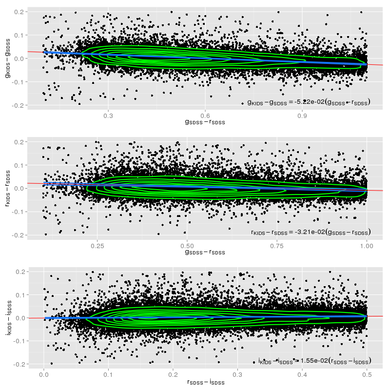
In the equatorial regions there is a deg2 overlap with SDSS, split between the SGC (deg2) and the NGC (deg2). In the SGC the overlap is at RA22h40-03h, and in the NGC it is at RA10h00-15h30,deg. We have compared (AB) colours of SDSS and ATLAS stars in the 120deg2 NGC overlap region to define the colour equations between the two systems. We use PSF magnitudes for SDSS and aperture 3 (corrected to total) magnitudes for ATLAS. The magnitude ranges used are , , , and .
In Fig. 11 we show , , , , . We see that the colour terms in and are almost negligible but there are small colour terms in . We find that:
We note that the zeropoint offsets with SDSS are small and due to slight differences in effective bandpass wavelengths. The exception is where the APASS AB zeropoints had to be fabricated from APASS . This is due to the non-linear (even double-valued for some star types) transformation really required when going from to . We have investigated if these offsets are caused by the method of magnitude measurement and find that these results are robust. Note that this issue in does not affect the AB magnitudes in Table 1 and Figs. 7, 9 and 10 since these are based on the original ESO Vega calibration plus the computed AB-Vega offsets given in Section 2.5.
We find good agreement in the colour coefficients with the SDSS-VST band conversions independently reported by the KiDS team at http://kids.strw.leidenuniv.nl/DR1/images/cterms.png as

Typical extinction coefficients (mags) for ATLAS are 0.46(), 0.19(), 0.09(), 0.05(), 0.05().
3.3 ATLAS-SDSS comparison
We next compare linearity of the ATLAS photometry (calibrated via nightly APASS and after the above colour corrections), with SDSS in the deg2 NGC overlap area. We shall see later that there are still some area-dependent zeropoint problems with the nightly APASS calibrations but here we will focus on the -band where the field-field problems are less. In the top panel of Fig. 12 we plot ATLAS aperture magnitudes versus model magnitudes for SDSS stars. The relation is consistent with linearity over the full mag range. In the middle panel of Fig. 12 we plot ATLAS Kron magnitudes against SDSS model magnitudes for galaxies. An offset to total of -0.15mag for galaxies is suggested for ATLAS. The relation appears noisier than the stars as expected but with no evidence of a scale error to . In the bottom panel of Fig. 12 we similarly plot ATLAS Petrosian magnitudes for galaxies against model magnitudes for SDSS. We see a reasonably linear, if noisier, relation. In the bin the rms error reaches , and mag for aperture, Petrosian and Kron magnitudes and here we might expect roughly equal contributions from ATLAS and SDSS. Overall, for VST ATLAS, we therefore recommend that aperture magnitudes (aper3) are used for stars while Petrosian or Kron magnitudes are used for galaxies.
These results for the band are typical of the results for the other 4 bands. These can be found at http://astro.dur.ac.uk/Cosmology/vstatlas/tests/.

3.4 ATLAS-Stripe 82 (WHDF field) comparison
Because SDSS only reaches a similar depth to ATLAS, it is not clear which survey is dominating the error spread at faint magnitudes. We have therefore also compared ATLAS photometry for galaxies and stars with the much deeper Stripe 82 (S82) photometry which lies within a 1deg2, specially observed, ATLAS area which also contains the William Herschel Deep Field (Metcalfe et al 2005) and again its deeper multi-epoch photometry allows a comparison to check the magnitude dependent error of the ATLAS photometry.
We note that although the WHDF ATLAS data has the same exposure as the ATLAS survey data and was taken in dark time, the seeing particularly in and is significantly worse than average (see Table 2). Indeed, the point source magnitude limits in all bands are brighter than the ATLAS average from mag in , to 0.64mag in and 0.54mag in (see Table 2). Nevertheless we can still make approximate checks of these brighter than usual WHDF ATLAS mag limits by comparison to deeper S82 data.
| Band | |||||
|---|---|---|---|---|---|
| Exposure | s | s | s | s | s |
| Airmass | |||||
| Seeing | |||||
| ATLAS Seeing | |||||
| Mag Lim | |||||
| ATLAS Mag Lim | |||||
| Sky Brightness | |||||
| ATLAS Sky Bri |

So in Fig. 13 we now show in the top panel the comparison between S82 model magnitudes and ATLAS aperture 3 magnitudes for point sources. Again the relation is linear with a low dispersion of mag at the WHDF ATLAS limit of from Table 2. Indeed, ATLAS aperture magnitudes in all bands show good agreement with the S82 magnitudes to their respective 5 limits from Table 2, confirming that the accuracy of these limits for point sources (see http://astro.dur.ac.uk/Cosmology/vstatlas/tests). The middle and bottom panels show the comparison between S82 model magnitudes and ATLAS Petrosian/Kron magnitudes now for SDSS galaxies. Both Petrosian and Kron magnitudes are reasonably linear but Petrosian appears to have a higher dispersion at of mag as opposed to mag for Kron. On this basis the preferred ATLAS magnitude for galaxy photometry again appears to be Kron magnitudes.
4 Zero-point comparisons with APASS and SDSS
4.1 APASS v ATLAS

We now move away from checks of the linearity of ATLAS photometry to address in more detail the question of the consistency of the ATLAS zeropoint calibration as discussed in Section 2.5 over wider areas of the survey. Maps of ESO ATLAS-APASS residuals in a deg2 area centred on RAh, Decdeg are shown in Fig. 14. The ATLAS data is calibrated from the ESO standards as used for the DR1 data release. The offsets in are obtained by extrapolating to from APASS and the offsets are from interpolating APASS and measurements. Offsets are seen that are clearly due to ATLAS/ESO calibration issues (generally in blocks of deg, corresponding to a single concatenation of tiles). Clearly some within field residuals are seen, particularly in (and ), that do not show any ATLAS characteristics and we believe that these may be due to problems in the APASS -band (and its extrapolation to ). The distribution of APASS-ATLAS (tile-by-tile) residuals for over a larger area is shown in Fig. 7 and the standard deviations are (), (), (), (), ().
4.2 ATLAS-SDSS Equatorial comparison
Figs. 15-19 show the residuals between the SDSS data for stars in the NGC overlap area at 10hRA15h30 and Decdeg assuming, in turn, the ESO calibration and the APASS nightly calibration for ATLAS. The SDSS magnitude ranges used are , , , and . The standard SDSS calibration was used here for simplicity, rather than the uber-calibration of Padmanabhan et al. (2008). As with the APASS comparison in Section 4.1, the ESO calibration clearly shows offsets on the scale of single concatenations. These are effectively removed by using the APASS nightly calibration. The ESO calibration also has larger residuals with clear VST nightly correlations. Some nights have no useable ESO standards and on these a long term average default value is used, perhaps explaining some of the stripes. However, even the APASS nightly calibration still has occasional issues with individual fields as can be seen in the band image. Also, we already noted that the APASS (and ) band photometry still has some issue from the ATLAS-APASS comparison above.
The distributions of SDSS-ATLAS residuals for individual stars in for ESO and APASS calibrations are compared in Fig. 20. Generally the APASS nightly calibrated data gives the smallest residuals with SDSS. The ESO calibration and the APASS individual fields calibration (not shown) appear to give larger residuals, in the latter case presumably due to statistical errors with the calibration based on fewer APASS stars. The ATLAS APASS nightly-SDSS mag standard deviations, measured on a tile-by-tile basis to reduce the effect of individual star random errors, are , , , and mag in , in most bands a significant improvement over the ESO ATLAS - SDSS comparison (, , , and in ). These standard deviations were measured on the basis of 183 tiles in and 112 tiles in . In both cases, the band result is affected by the presence of a single tile whose tile average is 0.66mag offset from the mean. Nevertheless in all bands the improvement gained from the APASS nightly calibration is clear.
Ultimately, for the final release, we shall calibrate ATLAS globally by incorporating the information from the overlaps in the RA and Dec directions on each field (Findlay et al. 2014b in prep.)


4.3 Star-galaxy separation comparisons
We now use the same NGC SDSS DR9 overlap area to compare ATLAS star-galaxy separation with that of SDSS. The results are shown in Fig. 21. Comparing top left and top right panels in the ATLAS Aper3-Petrosian : magnitude star-galaxy separation plane, we see that the ATLAS star-galaxy separation statistic has included some SDSS stars just above the stellar loci shown in the lower panels. These misclassified ATLAS stars have come from areas frequently coinciding with interchip gaps as can be seen in the upper panel of Fig. 22. The problem arises when the image quality varies slightly between the 2 sub-exposures and so the stellar locus is offset in the interchip areas when there is only one sub-exposure contributing to the image. Depending on the direction of the shift, this can result in stars being classified as galaxies. This problem will clearly be present in the ATLAS DR1 data. However, it is easy to fix this problem by plotting VST (Aper3-Petrosian) versus VST Petrosian for ATLAS classified galaxies and then remove the misclassified stars by a magnitude independent cut. This has the effect of cleaning up the mis-classified stars as shown in the lower panel of Fig. 22.


5 Galaxy and Star number counts
Adopting the corrected star - galaxy classifier, we next calculate the galaxy (and star) counts from 250deg2 in the deg range in the SGC which includes the SGP. Previously 2MASS counts have suggested evidence for a local underdensity in the SGP region. Here we simply focus on the counts to use their turnover to indicate the rough completeness limits of the survey. In Fig. 23 we compare these to a variety of previous galaxy counts compiled by Metcalfe et al. (2001). 2MASS counts suggest evidence for a local underdensity in the SGP region (Whitbourn & Shanks, 2014) but a fuller investigation of this issue using ATLAS data in a bigger area will be presented by Mackenzie et al (2014, in prep.). We see that the galaxy counts agree very well in most bands with other authors until the counts turn over due to incompleteness at faint magnitudes. This happens at AB mags , , , and . These are in reasonable agreement with the Mag Lim (gal) 5 limits for ATLAS given in Table 1. Star counts turn over at about the same limits but this is more dictated by the star-galaxy separation algorithm and is less related to more fundamental signal-to-noise considerations.

6 Access to ATLAS data
The ESO Science Archive provides a repository for data products released by the ESO Public Survey teams. Images and catalogues from ATLAS Data Release 1 can be retrieved from http://archive.eso.org/wdb/wdb/adp/phase3_main/form?phase3_collection=ATLAS&release_tag=1.
ATLAS data are also available through the OmegaCAM Science Archive (OSA, http://osa.roe.ac.uk), curated by the Wide-Field Astronomy Unit (WFAU) at the University of Edinburgh. Similar in design to the science archives developed by WFAU for sky survey data from UKIRT/WFCAM (Hambly et al., 2008) and VISTA (Cross et al., 2012), the OSA provides a range of access methods to both image and catalogue data products. It stores ATLAS catalogue data and image metadata in a relational database management system, which can be queried through the OSA web interface or using the Virtual Observatory (VO) Table Access Protocol (Dowler, Rixon, & Tody, 2011). Query results can be viewed within the OSA web interface or sent directly from it to VO-compliant desktop tools like Aladin (Bonnarel et al., 2000) and TOPCAT (Taylor, 2005), using the Simple Application Message Protocol (Taylor et al., 2012) standard. The OSA also integrates ATLAS catalogue data with a number of sky survey datasets, including SDSS, 2MASS, VHS and WISE, and provides the ATLAS consortium with access to proprietary data, as well as supporting use of ATLAS public data releases by the wider astronomical community.
7 Conclusions
We have described the basic characteristics of VST ATLAS. We find it meets its basic specification of comprising a ‘Southern Sloan’. This applies both to the median magnitude limits for point sources which are at least as deep as SDSS and to the median sky brightnesses which are comparable to SDSS. But in terms of its spatial resolution, the ATLAS survey presents essentially sub-arcsecond median seeing compared to the median imaging of SDSS.
We have derived the colour equations relating ATLAS stellar photometry to SDSS photometry. We find there are small but non-negligible colour terms, particularly in .
We have demonstrated the linearity of the ATLAS photometry by comparison in the 120deg2 NGC overlap area with SDSS. We recommend that radius (aperture 3) apertures are used for stellar photometry. For galaxies, ATLAS Kron magnitudes seem to give the most linear relations with SDSS model magnitudes. The same conclusions are found by comparing ATLAS and Stripe 82 photometry in the WHDF field. Here we found that the rms dispersions reached mag for stars at and mag for Kron galaxy magnitudes at mag
The current zeropoints assumed for come from APASS stellar photometry applied nightly and appear good to mag by comparison with SDSS data in overlap areas. We have investigated how area dependent these zeropoints are in the SDSS overlap area and find there are still small areas with residual errors. In the final global calibration we shall use the overlaps between tiles to reduce these errors.
We have tested the ATLAS star-galaxy separation by comparison with SDSS in the overlap areas and we found that 10% galaxies were misclassified as stars. We also found that 15% stars were misclassified as galaxies and that this higher rate was due to problems occurring in interchip gaps where only one sub-exposure was available. However, the problem is easily cured by using a more conservative star-galaxy separation line particularly at bright magnitudes.
Finally we also presented galaxy and star number counts in a 250deg2 area at the SGP and found where they turned over to define effective completeness limits. The galaxy counts turn over about at about our quoted 5 mag limits for galaxies. Star counts turn over at about the same limits but this is mainly dictated by the star-galaxy separation algorithm.
We conclude that the VST ATLAS is ready for scientific analysis. Currently the survey is 75% complete and it should be 100% complete by the end of 2015.
ACKNOWLEDGEMENTS
We are grateful to European Southern Observatory (ESO) and their associated service time VLT Survey Telescope observers for carrying out the ATLAS observations. We are indebted to the Cambridge Astronomical Surveys Unit (CASU) for reducing the ATLAS images and producing catalogues. We also acknowledge the work of the Wide Field Astronomy Unit (WFAU) at Edinburgh for archiving the ATLAS data. We also acknowledge use of publicly available SDSS data. This research has also made use of the APASS database, located at the AAVSO web site. Funding for APASS has been provided by the Robert Martin Ayers Sciences Fund.
References
- Belokurov et al. (2014) Belokurov V., Irwin M. J., Koposov S. E., Evans N. W., Gonzalez-Solares E., Metcalfe N., Shanks T., 2014, MNRAS, 441, 2124
- Bonnarel et al. (2000) Bonnarel F., et al., 2000, A&AS, 143, 33
- Bovy et al. (2012) Bovy J., et al., 2012, ApJ, 749, 41
- Bramich & Freudling (2012) Bramich D. M., Freudling W., 2012, MNRAS, 424, 1584
- Cross et al. (2012) Cross N. J. G., et al., 2012, A&A, 548, A119
- de Jong et al. (2013) de Jong J. T. A., et al., 2013, Msngr, 154, 44
- Dowler, Rixon, & Tody (2011) Dowler P., Rixon G., Tody D., 2011, arXiv, arXiv:1110.0497
- Edge et al. (2013) Edge A., Sutherland W., Kuijken K., Driver S., McMahon R., Eales S., Emerson J. P., 2013, Msngr, 154, 32
- Goto et al. (2002) Goto T., et al., 2002, PASJ, 54, 515
- Hambly et al. (2008) Hambly N. C., et al., 2008, MNRAS, 384, 637
- Irwin et al. (2004) Irwin M. J., et al., 2004, SPIE, 5493, 411
- Keenan, Barger, & Cowie (2013) Keenan R. C., Barger A. J., Cowie L. L., 2013, ApJ, 775, 62
- Koposov et al. (2014) Koposov S. E., Irwin M., Belokurov V., Gonzalez-Solares E., Yoldas A. K., Lewis J., Metcalfe N., Shanks T., 2014, MNRAS, 442, L85
- Kuijken et al (2011) Kuijken K. et al, 2011, Msngr, 146, 8
- McMahon et al. (2013) McMahon R. G., Banerji M., Gonzalez E., Koposov S. E., Bejar V. J., Lodieu N., Rebolo R., the VHS Collaboration, 2013, Msngr, 154, 35
- Merloni et al. (2012) Merloni A., et al., 2012, arXiv, arXiv:1209.3114
- Metcalfe et al. (2001) Metcalfe N., Shanks T., Campos A., McCracken H. J., Fong R., 2001, MNRAS, 323, 795
- Metcalfe et al. (2006) Metcalfe N., Shanks T., Weilbacher P. M., McCracken H. J., Fong R., Thompson D., 2006, MNRAS, 370, 1257
- Mountrichas & Shanks (2007) Mountrichas G., Shanks T., 2007, MNRAS, 380, 113
- Padmanabhan et al. (2008) Padmanabhan N., et al., 2008, ApJ, 674, 1217
- Sawangwit et al. (2010) Sawangwit U., Shanks T., Cannon R. D., Croom S. M., Ross N. P., Wake D. A., 2010, MNRAS, 402, 2228
- Schipani et al. (2012) Schipani P., et al., 2012, SPIE, 8444, 8441C
- Shanks et al. (2013) Shanks T., et al., 2013, Msngr, 154, 38
- Stoughton et al. (2002) Stoughton C., et al., 2002, AJ, 123, 485
- Taylor (2005) Taylor M. B., 2005, ASPC, 347, 29
- Taylor et al. (2012) Taylor M., et al., 2012, ivoa.spec, 1104
- Whitbourn, Shanks, & Sawangwit (2014) Whitbourn J. R., Shanks T., Sawangwit U., 2014, MNRAS, 437, 622
- Whitbourn & Shanks (2014) Whitbourn J. R., Shanks T., 2014, MNRAS, 437, 2146
- Wright et al. (2010) Wright E. L., et al., 2010, AJ, 140, 1868