跳到论文正文
W Papers独立论文阅读器 arXiv:1502.05388 论文正文 计算阅读时间 · 0%
引用这篇论文根据当前论文元数据生成,正式投稿前建议核对。


License: arXiv.org perpetual non-exclusive license
arXiv:1502.05388v2 [gr-qc] 29 Oct 2015

Boundary Terms for Causal Sets

Michel Bucka, Fay Dowkerb, Ian Jubbb and Sumati Suryac

aDepartment of Physics, Northeastern University, Boston, MA 02115, USA

bTheoretical Physics Group, Blackett Laboratory, Imperial College, London, SW7 2AZ, UK

cRaman Research Institute, CV Raman Ave, Sadashivanagar, Bangalore 560080, India

Abstract

We propose a family of boundary terms for the action of a causal set with a spacelike boundary. We show that in the continuum limit one recovers the Gibbons-Hawking-York boundary term in the mean. We also calculate the continuum limit of the mean causal set action for an Alexandrov interval in flat spacetime. We find that it is equal to the volume of the codimension-2 intersection of the two light-cone boundaries of the interval.

Contents

1 Introduction

One approach to constructing a quantum dynamics for the causal set approach to quantum gravity [1] is to discover a discrete counterpart of the gravitational action, S⁡[𝒞]S[\mathcal{C}] that can furnish the weight, ei​S​[𝒞]e^{iS[\mathcal{C}]}, of each causal set, 𝒞\mathcal{C}, in the gravitational sum over histories. A start in this direction has been made with a proposal for scalar curvature estimators for causal sets of dimension dd [2, 3, 4]. Summing such a scalar curvature estimator over all elements of a causal set (causet for short) gives a natural proposal for a causet analogue of the Einstein-Hilbert action, a proposal that remains to be studied in depth. The purpose of this paper is to initiate an investigation of gravitational boundary terms for the action of causets. This is likely to be important as, in the continuum, it is well known that the Einstein-Hilbert action, SE​HS_{EH}, is not the full story in the presence of spacetime boundaries. Indeed, the gravitational action must include a boundary term SG​H​YS_{GHY}, the Gibbons-Hawking-York (GHY) boundary term, in order to yield a well-defined variational principle when the metric is fixed on the boundary of spacetime [5, 6]. If the classical limit of quantum gravity is to arise from the path integral in the expected way, such a term in the action will be essential when boundaries are present. Whilst we do not yet know how to fix boundary conditions for causets in general, it is likely to be useful to have an analogue of the GHY boundary term for any causal set which is well-approximated by a manifold with a boundary. In this paper we initiate the study of boundary terms for causal sets by proposing an analogue in the case of spacelike boundaries and investigating the above mentioned causal set action for a causal interval with null boundaries. First we consider causal sets which are well approximated by (M,g)(M,g), a dd-dimensional, causal, Lorentzian spacetime with finite volume which admits a closed, compact spacelike submanifold, Σ\Sigma, such that the causal past and future sets, M±:=J±​(Σ)M^{\pm}:=J^{\pm}(\Sigma), satisfy M+∩M−=ΣM^{+}\cap M^{-}=\Sigma. Then Σ\Sigma is a component of the future (past) spacelike boundary for M−M^{-} (M+M^{+}) and the GHY term for Σ\Sigma, considered as a boundary of M+M^{+} or M−M^{-}, is given by

SG​H​Y[Σ,M±]=∓1lpd−2∫Σdd−1xhK,{S}_{GHY}\left[\Sigma,M^{\pm}\right]=\mp\frac{1}{l_{p}^{d-2}}\int_{\Sigma}d^{d-1}x\>\sqrt{h}\,K\>, (1)

where KK is the trace of the extrinsic curvature Kμ​ν=hμρ​hνσ​∇ρnσK_{\mu\nu}=h_{\mu}^{\rho}h_{\nu}^{\sigma}\nabla_{\rho}n_{\sigma} of Σ\Sigma, lp=(8​π​G)1d−2l_{p}=(8\pi G)^{\frac{1}{d-2}} is the rationalised Planck length and we are working in units where ℏ=1\hbar=1. Here we take nμn_{\mu} to be the future-pointing timelike unit covector normal to Σ\Sigma. We work with a mostly plus convention for the metric so nμn^{\mu} is past-pointing.

We recall that the integral in (1) is equal to the normal derivative of the volume of Σ\Sigma along the unit normal vector field, nμn^{\mu}:

∫Σdd−1​x​h​K=∂∂n​∫Σdd−1​x​h,\int_{\Sigma}d^{d-1}x\>\sqrt{h}\,K=\frac{\partial}{\partial n}\int_{\Sigma}d^{d-1}x\>\sqrt{h}\;, (2)

where this is the rate of change of the volume backwards in time, as nμn^{\mu} is past-pointing. This observation suggests a natural candidate for an analogue of the GHY boundary term for Σ\Sigma for a causet that can be faithfully embedded in MM. Spacetime volume corresponds to cardinality in a causet. Hence the spatial volume gradient corresponds intuitively to the difference between the number of causet elements that are future nearest neighbours of Σ\Sigma and the number of past nearest neighbours. This intuition turns out to be a good guide and we will identify a family of causal set boundary terms based on it. The family of causet boundary terms we find corresponds to the different ways to define a discrete derivative that tend to the same limit in the continuum. We will define the causet functions and state the claims about their continuum limits in section 2. The calculations justifying the claims appear in section 3. In section 4 we investigate the proposed causal set action for causal intervals in flat spacetime and show that its mean takes the form, in the continuum limit, of a boundary contribution from the codimension 2 “joint” of the interval’s boundary.

2 The Boundary Terms

Given a finite causet (𝒟,⪯)(\mathcal{D},\preceq), we define an “FkF_{k} element” to be an element of 𝒟\mathcal{D} with exactly kk elements -- not equal to itself -- to its future in the order11 1 Other ways to express this are, “has exactly kk descendants” and “precedes exactly kk elements excluding itself”. and define Fk​[𝒟]F_{k}\left[\mathcal{D}\,\right] to be the number of FkF_{k} elements in 𝒟\mathcal{D}. Similarly a “PkP_{k} element” is an element with exactly kk elements to its past in the order and Pk​[𝒟]P_{k}\left[\mathcal{D}\,\right] is the number of PkP_{k} elements in 𝒟\mathcal{D}. For example, F0​[𝒟]F_{0}[\mathcal{D}] (P0​[𝒟]P_{0}[\mathcal{D}]) is the number of maximal (minimal) elements of 𝒟\mathcal{D}.

Given a finite causet, (𝒞,⪯)(\mathcal{C},\preceq), with two subcausets, 𝒞+{\mathcal{C}}^{+} and 𝒞−{\mathcal{C}}^{-} we introduce the following family of causal set “boundary terms” (CBT):

SC​B​T(d)​[𝒞,𝒞−,𝒞+;p→,q→]:=(l/lp)d−2​ad​(∑mpm​Fm​[𝒞−]+∑nqn​Pn​[𝒞+]),S^{(d)}_{CBT}\left[\mathcal{C},\mathcal{C}^{-},\mathcal{C}^{+};\vec{p},\vec{q}\,\right]:=\left(l/l_{p}\right)^{d-2}a_{d}\left(\sum_{m}p_{m}F_{m}\left[\mathcal{C}^{-}\right]+\sum_{n}q_{n}P_{n}\left[\mathcal{C}^{+}\right]\right)\;, (3)

where the constant ada_{d} is given by

ad=d⁡(d+1)(d+2)​(Sd−2d⁡(d−1))2d.a_{d}=\frac{d(d+1)}{(d+2)}\left(\frac{S_{d-2}}{d(d-1)}\right)^{\frac{2}{d}}\;. (4)

Sd=(d+1)​πd+12/Γ⁡(d+12+1)S_{d}=(d+1)\pi^{\frac{d+1}{2}}/\Gamma\left(\frac{d+1}{2}+1\right) is the volume of the unit dd-sphere, ll is a length and lpl_{p} the Planck length defined previously. p→\vec{p} and q→\vec{q} denote finite strings of real numbers (p0,…,pm,…)(p_{0},\ldots,p_{m},\ldots) and (q0,…,qn,…)(q_{0},\ldots,q_{n},\ldots) respectively. We will prove that the strings must satisfy the following conditions:

∑mpm​Γ⁡(1d+m)m!+∑nqn​Γ⁡(1d+n)n!=0,\displaystyle\sum_{m}p_{m}\frac{\Gamma\left(\frac{1}{d}+m\right)}{m!}+\sum_{n}q_{n}\frac{\Gamma\left(\frac{1}{d}+n\right)}{n!}=0\;, (5)
∑mpm​Γ⁡(2d+m)m!−∑nqn​Γ⁡(2d+n)n!=1.\displaystyle\sum_{m}p_{m}\frac{\Gamma\left(\frac{2}{d}+m\right)}{m!}-\sum_{n}q_{n}\frac{\Gamma\left(\frac{2}{d}+n\right)}{n!}=1\;. (6)

We call (3) a boundary term but in general, when 𝒞+{\mathcal{C}}^{+} and 𝒞−{\mathcal{C}}^{-} are arbitrary subcausets of 𝒞\mathcal{C}, it will have no physical significance.

Let (M,g)(M,g) be a dd-dimensional spacetime with finite volume and spacelike, closed, compact hypersurface Σ\Sigma as described in the introduction. Given such a spacetime (M,g)(M,g) and sets M±:=J±​(Σ)M^{\pm}:=J^{\pm}(\Sigma), SC​B​T(d)S^{(d)}_{CBT} defines a family of random variables in the following way. The Poisson process of sprinkling points into MM with density ρ=l−d\rho=l^{-d} generates a random causet (𝒞,⪯)(\mathcal{C},\preceq) together with subcausets 𝒞±\mathcal{C}^{\pm} which consist of those elements sprinkled into M±M^{\pm}. The functions PkP_{k} and FkF_{k} acting on the random causets 𝒞+\mathcal{C}^{+} and 𝒞−\mathcal{C}^{-} respectively are random variables 𝐏k\mathbf{P}_{k} and 𝐅k\mathbf{F}_{k}. These random variables can be substituted into (3) to give the family of random variables SC​B​T(d)\textbf{S}^{(d)}_{CBT}:

SC​B​T(d)​[M,Σ,ρ;p→,q→]:=(l/lp)d−2​ad​(∑mpm​𝐅m+∑nqn​𝐏n).\textbf{S}^{(d)}_{CBT}\left[M,\Sigma,\rho;\vec{p},\vec{q}\,\right]:=\left(l/l_{p}\right)^{d-2}a_{d}\left(\sum_{m}p_{m}\mathbf{F}_{m}+\sum_{n}q_{n}\mathbf{P}_{n}\right)\;. (7)

We claim that in the limit of infinite density the expectation value, in the sprinkling process, of SC​B​T(d)\textbf{S}^{(d)}_{CBT} tends to the continuum GHY boundary term of the surface Σ\Sigma:

liml→0⟨SC​B​T(d)​[M,Σ,ρ;p→,q→]⟩=1lpd−2​∫Σdd−1​x​h​K=SG​H​Y​[Σ,M−],\lim_{l\rightarrow 0}\left\langle\textbf{S}^{(d)}_{CBT}[M,\Sigma,\rho;\vec{p},\vec{q}]\right\rangle=\frac{1}{l_{p}^{d-2}}\int_{\Sigma}d^{d-1}x\>\sqrt{h}\>K={S}_{GHY}\left[\Sigma,M^{-}\right]\;, (8)

where ⟨⋅⟩\langle\cdot\rangle denotes the mean over sprinklings. We will prove this in the next section.

One can see that at least two non-zero entries in p→\vec{p} and q→\vec{q} together are necessary in order to satisfy (5) and (6) and if exactly two entries are non-zero they will be uniquely fixed, but if more than two entries are non-zero this uniqueness is lost. This accords with the continuum boundary term being a first derivative. The freedom of choice in p→\vec{p} and q→\vec{q} is the freedom to discretise a derivative in many ways but the difference of two nearby values is sufficient.

We introduce special notation for the simplest member of the family:

S0(d)​[𝒞,𝒞−,𝒞+]:=(l/lp)d−2​ad2​Γ​(2d)​(F0​[𝒞−]−P0​[𝒞+]).S^{(d)}_{0}\left[\mathcal{C},\mathcal{C}^{-},\mathcal{C}^{+}\right]:=\left(l/l_{p}\right)^{d-2}\frac{a_{d}}{2\Gamma\left(\frac{2}{d}\right)}\left(F_{0}\left[\mathcal{C}^{-}\right]-P_{0}\left[\mathcal{C}^{+}\right]\right)\;. (9)

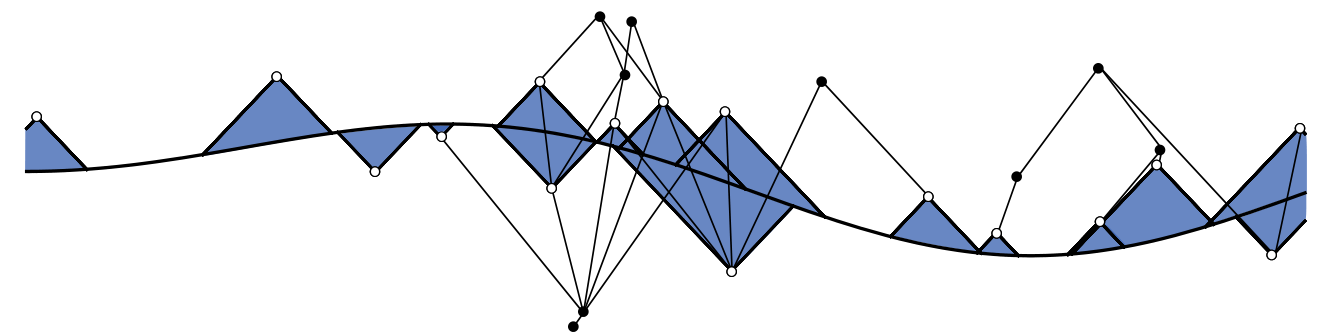
This is proportional to the difference in the numbers of minimal elements of 𝒞+\mathcal{C}^{+} and maximal elements of 𝒞−\mathcal{C}^{-}, and thus corresponds to the intuitive idea described in the introduction. An illustrative sketch of the idea is shown in Figure 1. This case is the easiest to investigate computationally, and we shall use its random variable counterpart, S0(d)​[M,Σ,ρ]\textbf{S}^{(d)}_{0}\left[M,\Sigma,\rho\right], later when we study the fluctuations of the discrete boundary terms numerically.
Refer to caption
Figure 1: An illustration of a sprinkling into a spacetime partitioned by a spacelike hypersurface. Black points correspond to causal set elements and links (irreducible causal relations) between elements are shown as thin black lines. The maximal (F0F_{0}) elements in 𝒞−\mathcal{C}^{-} and the minimal (P0P_{0}) elements in 𝒞+\mathcal{C}^{+} have been highlighted with white filling. The shaded areas illustrate the regions whose volumes V▲V_{\blacktriangle} and V▼V_{\blacktriangledown} are needed in the proof of Section 3. In this sketch P0=11P_{0}=11 and F0=5F_{0}=5 (with time flowing upwards).

There are two special subfamilies of boundary terms, one defined by p→=0\vec{p}=0 and the other by q→=0\vec{q}=0. In the former (latter) case, this corresponds to defining a boundary term for the past (future) boundary of 𝒞+\mathcal{C}^{+} (𝒞−\mathcal{C}^{-}) using only data from 𝒞+\mathcal{C}^{+} (𝒞−\mathcal{C}^{-}) itself. The simplest cases of these boundary terms are

S−(d)​[𝒞+]:=\displaystyle S^{(d)}_{-}[\mathcal{C}^{+}]:= (l/lp)d−2​adΓ⁡(2d)​(P0​[𝒞+]−d​P1​[𝒞+]),\displaystyle\left(l/l_{p}\right)^{d-2}\frac{a_{d}}{\Gamma\left(\frac{2}{d}\right)}\left(P_{0}\left[\mathcal{C}^{+}\,\right]-d\>P_{1}\left[\mathcal{C}^{+}\,\right]\right)\;, (10)
S+(d)​[𝒞−]:=\displaystyle S^{(d)}_{+}[\mathcal{C}^{-}]:= (l/lp)d−2​adΓ⁡(2d)​(d​F1​[𝒞−]−F0​[𝒞−]).\displaystyle\left(l/l_{p}\right)^{d-2}\frac{a_{d}}{\Gamma\left(\frac{2}{d}\right)}\left(d\>F_{1}\left[\mathcal{C}^{-}\,\right]-F_{0}\left[\mathcal{C}^{-}\,\right]\right)\;. (11)

These give rise to random variables S−(d)​[M,Σ,ρ]\textbf{S}^{(d)}_{-}[M,\Sigma,\rho] and S+(d)​[M,Σ,ρ]\textbf{S}^{(d)}_{+}[M,\Sigma,\rho] via sprinkling at density ρ=l−d\rho=l^{-d} as before.

2.1 The Surface Volume Family

We also propose a family of causet functions that will give the volume of a spacelike hypersurface in the appropriate context:

A(d)​[𝒞,𝒞−,𝒞+;p→,q→]:=(l/lp)d−1​bd​(∑mpm​Fm​[𝒞−]+∑nqn​Pn​[𝒞+]),A^{(d)}[\mathcal{C},\mathcal{C}^{-},\mathcal{C}^{+};\vec{p},\vec{q}]:=\left(l/l_{p}\right)^{d-1}b_{d}\left(\sum_{m}p_{m}F_{m}\left[\mathcal{C}^{-}\right]+\sum_{n}q_{n}P_{n}\left[\mathcal{C}^{+}\right]\right)\;, (12)

where

bd=d​(Sd−2d⁡(d−1))1d,b_{d}=d\left(\frac{S_{d-2}}{d(d-1)}\right)^{\frac{1}{d}}\;, (13)

and p→\vec{p} and q→\vec{q} now satisfy

∑mpm​Γ⁡(1d+m)m!+∑nqn​Γ⁡(1d+n)n!=1.\sum_{m}p_{m}\frac{\Gamma\left(\frac{1}{d}+m\right)}{m!}+\sum_{n}q_{n}\frac{\Gamma\left(\frac{1}{d}+n\right)}{n!}=1\;. (14)

We see that only one non-zero entry is necessary to give an expression for the discrete surface volume. Once again, for (M,g)(M,g), Σ\Sigma and ρ=l−d\rho=l^{-d}, we can define a family of random variables,

A(d)​[M,Σ,ρ;p→,q→]:=(l/lp)d−2​bd​(∑mpm​𝐅m+∑nqn​𝐏n).\textbf{A}^{(d)}\left[M,\Sigma,\rho;\vec{p},\vec{q}\,\right]:=\left(l/l_{p}\right)^{d-2}b_{d}\left(\sum_{m}p_{m}\mathbf{F}_{m}+\sum_{n}q_{n}\mathbf{P}_{n}\right)\;. (15)

We claim that, in the limit of infinite density, the expectation value of A(d)\textbf{A}^{(d)} in the sprinkling process tends to the spatial volume of the surface Σ\Sigma:

liml→0⟨A(d)​[M,Σ,ρ;p→,q→]⟩=1lpd−1​∫Σdd−1​x​h.\lim_{l\rightarrow 0}\left\langle\textbf{A}^{(d)}[M,\Sigma,\rho;\vec{p},\vec{q}]\right\rangle=\frac{1}{l_{p}^{d-1}}\int_{\Sigma}d^{d-1}x\>\sqrt{h}\;. (16)

In proving (8) we will establish the results necessary to prove this claim as well.

One can define functions for the volumes of future and past boundaries respectively as the two simplest members of the family:

A+(d)​[𝒞−]:=\displaystyle A^{(d)}_{+}[\mathcal{C}^{-}]:= (l/lp)d−1​bdΓ⁡(1d)​F0​[𝒞−],\displaystyle\left(l/l_{p}\right)^{d-1}\frac{b_{d}}{\Gamma\left(\frac{1}{d}\right)}\>F_{0}[\mathcal{C}^{-}]\;, (17)
A−(d)​[𝒞+]:=\displaystyle A^{(d)}_{-}[\mathcal{C}^{+}]:= (l/lp)d−1​bdΓ⁡(1d)​P0​[𝒞+].\displaystyle\left(l/l_{p}\right)^{d-1}\frac{b_{d}}{\Gamma\left(\frac{1}{d}\right)}\>P_{0}[\mathcal{C}^{+}]\;. (18)

3 Calculations

3.1 ⟨𝐅m⟩\left\langle\mathbf{F}_{m}\right\rangle and ⟨𝐏m⟩\left\langle\mathbf{P}_{m}\right\rangle for Poisson Sprinklings

In order to establish (8) and (16) we will find the behaviour of the mean values of 𝐅m\mathbf{F}_{m} and 𝐏m\mathbf{P}_{m} as ρ\rho tends to infinity (l→0l\rightarrow 0). The result will follow almost immediately.

For any given realisation of the sprinkling, the probability that a sprinkled point p∈M−p\in M^{-} below the surface Σ\Sigma is an FkF_{k} element of M−M^{-} is given by the probability that kk points of the sprinkling lie in the region J+​(p)∩J−​(Σ)J^{+}(p)\cap J^{-}(\Sigma). The Poisson process assigns a probability,

ℙ⁡(k points in ​J+​(p)∩J−​(Σ))=(ρ​V▼​(p))kk!​e−ρ​V▼​(p),\mathbb{P}\left(\text{k points in }J^{+}(p)\cap J^{-}(\Sigma)\right)=\frac{\left(\rho\>V_{\blacktriangledown}(p)\right)^{k}}{k!}e^{-\rho V_{\blacktriangledown}(p)}\;, (19)

to this event, where V▼​(p):=vol⁡(J+​(p)∩J−​(Σ))V_{\blacktriangledown}(p):=\mathrm{vol}(J^{+}(p)\cap J^{-}(\Sigma)) is the spacetime volume of the region J+​(p)∩J−​(Σ)J^{+}(p)\cap J^{-}(\Sigma). The probability of sprinkling an element into an infinitesimal dd-volume d​VpdV_{p} at pp is ρ​d​Vp\rho dV_{p} where ρ=l−d\rho=l^{-d} is the sprinkling density, and so the total expected number of FkF_{k} elements below Σ\Sigma is

⟨𝐅k⟩=ρ​∫J−​(Σ)d​Vp​(ρ​V▼​(p))kk!​e−ρ​V▼​(p).\left\langle\mathbf{F}_{k}\right\rangle=\rho\int_{J^{-}(\Sigma)}dV_{p}\;\frac{\left(\rho\>V_{\blacktriangledown}(p)\right)^{k}}{k!}e^{-\rho V_{\blacktriangledown}(p)}\;. (20)

Similarly the expected number of PkP_{k} elements above Σ\Sigma is

⟨𝐏k⟩=ρ​∫J+​(Σ)d​Vp​(ρ​V▲​(p))kk!​e−ρ​V▲​(p),\left\langle\mathbf{P}_{k}\right\rangle=\rho\int_{J^{+}(\Sigma)}dV_{p}\;\frac{\left(\rho\>V_{\blacktriangle}(p)\right)^{k}}{k!}e^{-\rho V_{\blacktriangle}(p)}\;, (21)

where V▲​(p):=vol​(J+​(Σ)∩J−​(p))V_{\blacktriangle}(p):=\textrm{vol}(J^{+}(\Sigma)\cap J^{-}(p)).

Let xμ=(t,𝐱)x^{\mu}=(t,\mathbf{x}) be “synchronous” or Gaussian Normal Coordinates (GNCs) adapted to Σ\Sigma such that in a neighbourhood UΣU_{\Sigma} of Σ\Sigma the line element is

d​s2=−d​t2+hi​j​(t,𝐱)​d​xi​d​xj.ds^{2}=-dt^{2}+h_{ij}(t,\mathbf{x})dx^{i}dx^{j}\;. (22)

In these coordinates the surface Σ\Sigma corresponds to t=0t=0. Each point pp in the neighbourhood lies on a unique timelike geodesic whose tangent vector at Σ\Sigma is equal to −nμ-n^{\mu} on Σ\Sigma, and the tt coordinate of pp is equal to the proper time from Σ\Sigma to pp along that geodesic. The spacetime (M,g)({M},g) restricted to this neighbourhood of Σ\Sigma is globally hyperbolic and Σ\Sigma is a Cauchy surface within it.

The integrals (20) and (21) seem intractable as they stand, since the integration is over the entire causal past/future of the surface. However, since Σ\Sigma is closed and compact and M+M^{+} and M−M^{-} are of finite volume, we can always find a subneighbourhood of UΣU_{\Sigma} such that the contribution to the integrals from the complement of that subneighbourhood tends to zero exponentially quickly as ρ→∞\rho\rightarrow\infty. Let ε>0\varepsilon>0 be small enough such that for all p∈Σp\in\Sigma and |t|<ε|t|<\varepsilon, (t,𝐱⁡(p))(t,\mathbf{x}(p)) are the GNCs of a point in UΣU_{\Sigma}. Define UΣ​(ε):={q∈UΣ:|t⁡(q)|<ε}U_{\Sigma}(\varepsilon):=\{q\in U_{\Sigma}:|t(q)|<\varepsilon\} and consider the integral in (21) restricted to W:=J+​(Σ)∖UΣ​(ε)W:=J^{+}(\Sigma)\setminus U_{\Sigma}(\varepsilon):

|∫Wd​Vp​(ρ​V▲​(p))kk!​e−ρ​V▲​(p)|≤‖e−ρ​V▲‖​∫Wd​Vp​(ρ​V▲​(p))kk!,\Big|\,\int_{W}dV_{p}\;\frac{\left(\rho\>V_{\blacktriangle}(p)\right)^{k}}{k!}e^{-\rho V_{\blacktriangle}(p)}\Big|\leq\|e^{-\rho V_{\blacktriangle}}\|\int_{W}dV_{p}\;\frac{\left(\rho\>V_{\blacktriangle}(p)\right)^{k}}{k!}\;, (23)

where ‖e−ρ​V▲‖\|e^{-\rho V_{\blacktriangle}}\| is the uniform norm over the integration region WW. Since V▲​(p)V_{\blacktriangle}(p) increases with tt along the geodesics from Σ\Sigma, and {xμ∈UΣ:t=ε}\{x^{\mu}\in U_{\Sigma}\,:\,t=\varepsilon\} is homeomorphic to Σ\Sigma and so is closed and compact, V▲​(p)V_{\blacktriangle}(p) achieves its minimum value Vm​i​n>0V_{min}>0 in WW at some point with t=εt=\varepsilon. Then ‖e−ρ​V▲‖=e−ρ​Vm​i​n\|e^{-\rho V_{\blacktriangle}}\|=e^{-\rho V_{min}} and so the integral (23) falls off exponentially fast as ρ→∞\rho\rightarrow\infty. Similarly for (20).

Thus, so long as ρ\rho is large enough, we make only an exponentially small error by cutting off the integration ranges in (20) and (21) at t=±εt=\pm\varepsilon with ε\varepsilon as small as we need in order to be able to expand in powers of tt. Expanding the determinant of the metric around t=0t=0, the integrals we want to evaluate are

⟨𝐅k⟩=ρ​∫Σdd−1​x​∫−ε0d​t​h12​(1+12​h˙h​t+O⁡(t2))​(ρ​V▼​(p))kk!​e−ρ​V▼​(t,𝐱)+…,⟨𝐏k⟩=ρ​∫Σdd−1​x​∫0εd​t​h12​(1+12​h˙h​t+O⁡(t2))​(ρ​V▲​(p))kk!​e−ρ​V▲​(t,𝐱)+…,\displaystyle\begin{aligned} \left\langle\mathbf{F}_{k}\right\rangle&=\rho\int_{\Sigma}d^{d-1}x\int_{-\varepsilon}^{0}dt\>h^{\frac{1}{2}}\left(1+\frac{1}{2}\frac{\dot{h}}{h}t+O(t^{2})\right)\frac{\left(\rho\>V_{\blacktriangledown}(p)\right)^{k}}{k!}e^{-\rho V_{\blacktriangledown}(t,\mathbf{x})}+\dots\;,\\ \left\langle\mathbf{P}_{k}\right\rangle&=\rho\int_{\Sigma}d^{d-1}x\int_{0}^{\varepsilon}dt\>h^{\frac{1}{2}}\left(1+\frac{1}{2}\frac{\dot{h}}{h}t+O(t^{2})\right)\frac{\left(\rho\>V_{\blacktriangle}(p)\right)^{k}}{k!}e^{-\rho V_{\blacktriangle}(t,\mathbf{x})}+\dots\;,\end{aligned} (24)

where both h:=d​e​t​(hi​j)h:=det\left(h_{ij}\right) and h˙:=∂h∂t\dot{h}\>:=\frac{\partial h}{\partial t} are evaluated at t=0t=0, and +…+\dots denotes “terms that vanish exponentially fast in the limit ρ→∞\rho\rightarrow\infty”.

3.2 Volumes

Let us first calculate V▲​(p)V_{\blacktriangle}(p), the volume of region 𝒳p:=J−​(p)∩M+\mathcal{X}_{p}:=J^{-}(p)\cap M^{+}, for pp in UΣ​(ε)∩M+U_{\Sigma}(\varepsilon)\cap M^{+}. Let p0p_{0} be the point on Σ\Sigma where the unique timelike geodesic through pp whose tangent is normal to Σ\Sigma intersects Σ\Sigma. Let the values of pp’s GNCs be xpμ=(tp,𝐱p)x^{\mu}_{p}=(t_{p},\mathbf{x}_{p}), then p0p_{0} has GNCs x0μ:=xμ​(p0)=(0,𝐱p)x_{0}^{\mu}:=x^{\mu}(p_{0})=(0,\mathbf{x}_{p}). We choose ε\varepsilon small enough that, for every p∈UΣ​(ε)∩M+p\in U_{\Sigma}(\varepsilon)\cap M^{+}, there exists a Riemann normal neighbourhood centred on p0p_{0} containing the region J−​(p)∩M+J^{-}(p)\cap M^{+}. We choose Riemann Normal Coordinates (RNCs) centered at p0p_{0}, yμ¯=(y0¯,𝐲)=(t¯,𝐲)y^{\overline{\mu}}=(y^{\overline{0}},\mathbf{y})=(\overline{t},\mathbf{y}), such that the GNC time coordinate of pp equals the RNC time coordinate of pp: tp=t¯p=:Tt_{p}=\overline{t}_{p}=:T.

The relationship between RNCs yμ¯y^{\overline{\mu}} and GNCs xνx^{\nu} is, to second order,

yμ¯=Aνμ¯​(xν−x0ν)+12​Aμμ¯​Γν​ρμ​(p0)​(xν−x0ν)​(xρ−x0ρ)+O⁡((x−x0)3).y^{\overline{\mu}}=A^{\overline{\mu}}_{\;\nu}(x^{\nu}-x_{0}^{\nu})+\frac{1}{2}A^{\overline{\mu}}_{\;\mu}\Gamma^{\mu}_{\;\nu\rho}(p_{0})(x^{\nu}-x_{0}^{\nu})(x^{\rho}-x_{0}^{\rho})+O((x-x_{0})^{3})\;. (25)

The constant matrix Aμμ¯A^{\overline{\mu}}_{\;\mu} obeys

Aμμ¯​Aνν¯​ημ¯​ν¯=gμ​ν​(p0),A^{\overline{\mu}}_{\;\mu}A^{\overline{\nu}}_{\;\nu}\eta_{\overline{\mu}\overline{\nu}}=g_{\mu\nu}(p_{0})\;, (26)

and the metric and Christoffel symbols in RNCs are flat at p0p_{0}:

gμ¯​ν¯​(p0)\displaystyle g_{\overline{\mu}\overline{\nu}}(p_{0}) =ημ¯​ν¯,\displaystyle=\eta_{\overline{\mu}\overline{\nu}}\;, (27)
Γν¯​ρ¯μ¯​(p0)\displaystyle\Gamma^{\overline{\mu}}_{\;\overline{\nu}\overline{\rho}}(p_{0}) =0.\displaystyle=0\;.

The inverse coordinate transformation is

xμ=x0μ+Aμ¯μ​yμ¯+O⁡(y3),x^{\mu}=x_{0}^{\mu}+A^{\mu}_{\;\overline{\mu}}y^{\overline{\mu}}+O(y^{3})\;, (28)

where Aμ¯μA^{\mu}_{\;\overline{\mu}} is the inverse matrix of Aμμ¯A^{\overline{\mu}}_{\;{\mu}}, i.e. Aμμ¯​Aν¯μ=δν¯μ¯A^{\overline{\mu}}_{\;\mu}A^{\mu}_{\;\overline{\nu}}=\delta^{\overline{\mu}}_{\;\overline{\nu}} and Aμ¯μ​Aνμ¯=δνμA^{\mu}_{\;\overline{\mu}}A^{\overline{\mu}}_{\;\nu}=\delta^{\mu}_{\;\nu}. There is no O⁡(y2)O(y^{2}) term in (28) due to the fact that Γν¯​ρ¯μ¯​(p0)=0\Gamma^{\overline{\mu}}_{\;\overline{\nu}\overline{\rho}}(p_{0})=0. The components of Aμμ¯A^{\overline{\mu}}_{\mu} satisfy A 00¯=1A^{\overline{0}}_{\;0}=1, Ai0¯=0A^{\overline{0}}_{\;i}=0, Ai​ı¯​Aj​ȷ¯​δ​ı¯​​ȷ¯=hi​j​(p0)A^{{\overline{\emph{\char 16\relax}}}}_{\;i}A^{{\overline{\emph{\char 17\relax}}}}_{\;j}\delta_{{\overline{\emph{\char 16\relax}}}{\overline{\emph{\char 17\relax}}}}=h_{ij}(p_{0}) and δ​ı¯​​ȷ¯=A​ı¯i​A​ȷ¯j​hi​j​(p0)\delta_{{\overline{\emph{\char 16\relax}}}{\overline{\emph{\char 17\relax}}}}=A^{i}_{\;{\overline{\emph{\char 16\relax}}}}A^{j}_{\;{\overline{\emph{\char 17\relax}}}}h_{ij}(p_{0}).

As we saw above, the limit we are considering, ρ→∞\rho\rightarrow\infty, allows us to take ε\varepsilon to be arbitrarily small so the limit can be thought of as driving each relevant p→p0p\rightarrow p_{0} on Σ\Sigma along the geodesic normal to Σ\Sigma. That makes the region 𝒳p\mathcal{X}_{p}, whose volume we need, tend to a truncated solid, nearly flat cone with apex pp and a base on Σ\Sigma defined by a quadratic form in the three spatial RNCs around p0p_{0}. The leading contribution to the volume,

V▲​(p)=∫𝒳pdd​y​−g⁡(y),V_{\blacktriangle}(p)=\int_{\mathcal{X}_{p}}d^{d}y\;\sqrt{-g(y)}\;, (29)

is therefore the volume, Sd−2d⁡(d−1)​Td\frac{S_{d-2}}{d(d-1)}T^{d}, of the flat cone of height TT with a flat base on surface t¯=0\overline{t}=0. Corrections to this are higher order in TT and come from three sources: (i) −g⁡(y)≠1\sqrt{-g(y)}\neq 1, (ii) the null geodesics down from pp to Σ\Sigma forming the top boundary, Tp:=∂J−​(p)∩M+T_{p}:=\partial J^{-}(p)\cap M^{+}, of 𝒳p\mathcal{X}_{p} are not straight, and (iii) the base, Bp:=Σ∩J−​(p)B_{p}:=\Sigma\cap J^{-}(p) is not a flat disc. The first two corrections are due to the curvature of MM and the third comes from the extrinsic curvature of Σ\Sigma.

The correction from (iii) is found by taking spacetime to be flat, so that RNCs are the usual Cartesian coordinates centred at p0p_{0} and TpT_{p} is the top boundary of the flat cone, satisfying ∑​ı=1d−1(y​ı¯)2=(T−t¯)2\sum_{\emph{\char 16\relax}=1}^{d-1}\left(y^{\overline{\emph{\char 16\relax}}}\right)^{2}=(T-\overline{t})^{2} and t¯∈[0,T]\overline{t}\in[0,T]. The base BpB_{p} in GNCs lies in surface t=0t=0, so we can use (25) to find the equation for the surface in RNCs. This gives

t¯=12​Γi​j0​(p0)​(xi−x0i)​(xj−x0j)+O⁡((x−x0)3).\overline{t}=\frac{1}{2}\Gamma^{0}_{\;ij}(p_{0})(x^{i}-x_{0}^{i})(x^{j}-x_{0}^{j})+O((x-x_{0})^{3})\;. (30)

The linear part on the right hand side of (25) vanishes, since Aμ0¯​(xμ−x0μ)=tA^{\overline{0}}_{\;\mu}(x^{\mu}-x_{0}^{\mu})=t (which follows from Ai0¯=0A^{\overline{0}}_{\;i}=0 and A 00¯=1A^{\overline{0}}_{\;0}=1) and t=0t=0 on the bottom surface. Using the inverse RNC relation (28), the equation for BpB_{p} in RNCs is

t¯=12​Γi​j0​(p0)​A​ı¯i​A​ȷ¯j​y​ı¯​y​ȷ¯+O⁡(y3).\overline{t}=\frac{1}{2}\Gamma^{0}_{\;ij}(p_{0})A^{i}_{\;{\overline{\emph{\char 16\relax}}}}A^{j}_{\;{\overline{\emph{\char 17\relax}}}}y^{{\overline{\emph{\char 16\relax}}}}y^{{\overline{\emph{\char 17\relax}}}}+O(y^{3})\;. (31)

Let us rewrite this equation in spherical polar coordinates, i.e. define r:=δ​ı¯​​ȷ¯​y​ı¯​y​ȷ¯r:=\sqrt{\delta_{{\overline{\emph{\char 16\relax}}}{\overline{\emph{\char 17\relax}}}}y^{\overline{\emph{\char 16\relax}}}y^{\overline{\emph{\char 17\relax}}}} and the usual angular coordinates ϕ1,..,ϕd−2\phi_{1},..,\phi_{d-2} in terms of the spatial coordinates y1¯=rcos(ϕ1),…,yd−1¯=rsin(ϕ1)⋯sin(ϕd−3)sin(ϕd−2)y^{\overline{1}}=r\cos(\phi_{1}),\ldots,y^{\overline{d-1}}=r\sin(\phi_{1})\cdots\sin(\phi_{d-3})\sin(\phi_{d-2}). Then

t¯=12​(Γi​j0​(p0)​A​ı¯i​A​ȷ¯j​y​ı¯​y​ȷ¯r2)​r2+O⁡(y3)=12​f​(𝐱p,ϕ)​r2+O⁡(y3),\overline{t}=\frac{1}{2}\left(\Gamma^{0}_{\;ij}(p_{0})A^{i}_{\;{\overline{\emph{\char 16\relax}}}}A^{j}_{\;{\overline{\emph{\char 17\relax}}}}\frac{y^{{\overline{\emph{\char 16\relax}}}}y^{{\overline{\emph{\char 17\relax}}}}}{r^{2}}\right)r^{2}+O(y^{3})=\frac{1}{2}f(\mathbf{x}_{p},{\boldsymbol{\phi}})r^{2}+O(y^{3})\;, (32)

where ϕ\boldsymbol{\phi} stands collectively for all the angular coordinates ϕ1,..,ϕd−2\phi_{1},..,\phi_{d-2}. The function f⁡(𝐱p,ϕ)f(\mathbf{x}_{p},\boldsymbol{\phi}) depends on 𝐱p\mathbf{x}_{p} since Γi​j0\Gamma^{0}_{\;ij} and A​ı¯iA^{i}_{\;{\overline{\emph{\char 16\relax}}}} depend on p0p_{0}.

With the boundaries of the integration region in hand, we can now write down the integral explicitly in spherical coordinates:

∫𝒳p​in flat spacedd​y=∫Sd−2d​Ωd−2​∫0rm​a​x​(ϕ)rd−2​𝑑r​∫12​f​(𝐱p,ϕ)​r2−r+T𝑑t¯+O⁡(Td+2),\int_{\mathcal{X}_{p}\ \textrm{in flat space}}d^{d}y=\int_{S^{d-2}}d\Omega_{d-2}\int_{0}^{r_{max}(\phi)}r^{d-2}dr\int_{\frac{1}{2}f(\mathbf{x}_{p},\phi)r^{2}}^{-r+T}d\overline{t}+O(T^{d+2})\;, (33)

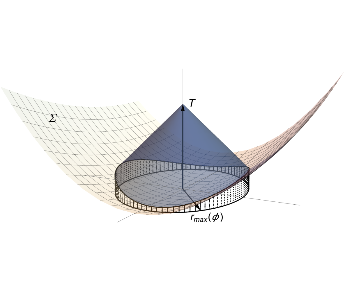
where rm​a​x​(ϕ)r_{max}(\boldsymbol{\phi}) is the value of the radial coordinate for which BpB_{p} intersects TpT_{p} at an angle ϕ\boldsymbol{\phi}, as shown in Figure 2. Equating the time coordinates of TpT_{p} and BpB_{p} gives

12​f​(𝐱p,ϕ)​rm​a​x2​(ϕ)=−rm​a​x​(ϕ)+T.\frac{1}{2}f(\mathbf{x}_{p},\boldsymbol{\phi}){r_{max}}^{2}(\boldsymbol{\phi})=-r_{max}(\boldsymbol{\phi})+T\;. (34)

We

Refer to caption
Figure 2: A 33-dimensional representation of the region 𝒳p\mathcal{X}_{p} in RNCs. The top, TpT_{p}, of ∂𝒳p\partial\mathcal{X}_{p} can be approximated as a flat cone, and the base, BpB_{p}, intersects TpT_{p} at a radial coordinate, rm​a​x​(ϕ)r_{max}(\boldsymbol{\phi}), which will in general be a function of the angles ϕ\boldsymbol{\phi} (in 33 dimensions there is one angle ϕ\phi). This function is found by projecting down from the intersection to the t¯\overline{t} plane.

solve this for rm​a​x​(ϕ)r_{max}(\boldsymbol{\phi}) and take the positive solution. The solution can be expanded in TT and is simply rm​a​x=T+O⁡(T2)r_{max}=T+O(T^{2}), with angular dependent terms contributing at O⁡(T2)O(T^{2}). The O⁡(T2)O(T^{2}) term will contribute at O⁡(Td+2)O(T^{d+2}) in the volume integral. Substituting rm​a​x=Tr_{max}=T into (33) allows us to evaluate the integral (33), which equals

Sd−2d⁡(d−1)​Td​(1−d2​(d+1)​Γi​j0​(p0)​A​ı¯i​A​ȷ¯j​δ​ı¯​​ȷ¯​T)+O⁡(Td+2),\frac{S_{d-2}}{d(d-1)}T^{d}\left(1-\frac{d}{2(d+1)}\Gamma^{0}_{\;ij}(p_{0})A^{i}_{\;{\overline{\emph{\char 16\relax}}}}A^{j}_{\;{\overline{\emph{\char 17\relax}}}}\delta^{{\overline{\emph{\char 16\relax}}}{\overline{\emph{\char 17\relax}}}}T\right)+O(T^{d+2})\;, (35)

where the δ​ı¯​​ȷ¯\delta^{{\overline{\emph{\char 16\relax}}}{\overline{\emph{\char 17\relax}}}} comes from the fact that cross terms (​ı¯≠​ȷ¯{\overline{\emph{\char 16\relax}}}\neq{\overline{\emph{\char 17\relax}}}) vanish under the angular integration. The defining relations for A​ı¯iA^{i}_{\;{\overline{\emph{\char 16\relax}}}} can be rearranged to give A​ı¯i​A​ȷ¯j​δ​ı¯​​ȷ¯=hi​j​(p0)A^{i}_{\;{\overline{\emph{\char 16\relax}}}}A^{j}_{\;{\overline{\emph{\char 17\relax}}}}\delta^{{\overline{\emph{\char 16\relax}}}{\overline{\emph{\char 17\relax}}}}=h^{ij}(p_{0}), and in GNCs the extrinsic curvature on the surface is given by

K=gμ​ν​∇μnν=−Γi​j0​hi​j=−12​h˙h.K=g^{\mu\nu}\nabla_{\mu}n_{\nu}=-\Gamma^{0}_{\;ij}h^{ij}=-\frac{1}{2}\frac{\dot{h}}{h}\;. (36)

Substituting this into (35) we obtain

Sd−2d⁡(d−1)​Td​(1+d2​(d+1)​K​(0,𝐱p)​T)+O⁡(Td+2),\frac{S_{d-2}}{d(d-1)}T^{d}\left(1+\frac{d}{2(d+1)}K(0,\mathbf{x}_{p})T\right)+O(T^{d+2})\;, (37)

and we see the first contribution is the volume of the flat cone with flat base as expected, and the first correction is of order Td+1T^{d+1}.

The corrections (i) and (ii) come from the non-flatness of the metric. The determinant −g\sqrt{-g} can be expanded in RNCs and the deviation of TpT_{p} from straight lines considered. The curvature contribution to the volume of a small, approximately flat causal interval – or Alexandrov neighbourhood – of these effects has been calculated [7, 8, 9] and the same arguments show that the corrections (i) and (ii) in our case are of the same order, O⁡(Td+2)O(T^{d+2}), which means they are suppressed with respect to the correction derived above. This is to be expected on dimensional grounds as extrinsic curvature has dimensions of inverse length whereas Riemann curvature has dimensions of inverse length squared. We will see that (Td+2)(T^{d+2}) corrections do not contribute to the boundary term in the limit.

So we have

V▲​(T,𝐱)=Sd−2d⁡(d−1)​Td​(1+d2​(d+1)​K​(0,𝐱)​T)+O⁡(Td+2).V_{\blacktriangle}(T,\mathbf{x})=\frac{S_{d-2}}{d(d-1)}T^{d}\left(1+\frac{d}{2(d+1)}K(0,\mathbf{x})T\right)+O(T^{d+2})\;. (38)

The same calculation for p∈UΣ​(ε)∩M−p\in U_{\Sigma}(\varepsilon)\cap M^{-} gives

V▼​(−T,𝐱)=Sd−2d⁡(d−1)​Td​(1−d2​(d+1)​K​(0,𝐱)​T)+O⁡(Td+2),V_{\blacktriangledown}(-T,\mathbf{x})=\frac{S_{d-2}}{d(d-1)}T^{d}\left(1-\frac{d}{2(d+1)}K(0,\mathbf{x})T\right)+O(T^{d+2})\;, (39)

where T>0T>0.

3.3 The Mean of SC​B​T(d)\textbf{S}^{(d)}_{CBT}

Focussing on ⟨𝐏k⟩\left\langle\mathbf{P}_{k}\right\rangle, we use (38) in (24) to find

⟨𝐏k⟩=ρk+1​Akk!​∫Σdd−1​x​h12​∫0εd​t​[(td​k+(k​B−K)​td​k+1)+O⁡(td​k+2)]​e−ρ​A​td−ρk+2​Ak+1k!∫Σdd−1xh12∫0εdt[Btd​k+d+1+O(td​k+d+2)]e−ρ​A​td+…,\displaystyle\begin{aligned} \left\langle\mathbf{P}_{k}\right\rangle&=\frac{\rho^{k+1}A^{k}}{k!}\int_{\Sigma}d^{d-1}x\>h^{\frac{1}{2}}\int_{0}^{\varepsilon}dt\>\left[\left(t^{dk}+\left(kB-K\right)t^{dk+1}\right)+O\left(t^{dk+2}\right)\right]e^{-\rho A\>t^{d}}\\ &-\frac{\rho^{k+2}A^{k+1}}{k!}\int_{\Sigma}d^{d-1}x\>h^{\frac{1}{2}}\int_{0}^{\varepsilon}dt\>\left[Bt^{dk+d+1}+O\left(t^{dk+d+2}\right)\right]e^{-\rho A\>t^{d}}+\dots\;,\end{aligned} (40)

where K:=K⁡(0,𝐱)K:=K(0,\mathbf{x}) and we have defined

A:=Sd−2d⁡(d−1),B:=d2​(d+1)​K.\displaystyle\begin{aligned} A&:=\frac{S_{d-2}}{d(d-1)}\;,\\ B&:=\frac{d}{2(d+1)}K\;.\end{aligned} (41)

To find out how this behaves in the limit of ρ→∞\rho\rightarrow\infty, it suffices to find the behaviour of the following integral:

ρp​∫0εd​t​tq​e−ρ​A​td,\rho^{p}\int_{0}^{\varepsilon}dt\ t^{q}e^{-\rho At^{d}}\;, (42)

where p,q∈ℝp,q\in\mathbb{R}. We make the substitution z=ρ​A​tdz=\rho At^{d} to put (42) into the form of an incomplete gamma function.

A−(q+1d)d​ρp−(q+1d)​∫0ρ​A​εdd​z​z(q+1d)−1​e−z.\frac{A^{-\left(\frac{q+1}{d}\right)}}{d}\rho^{p-\left(\frac{q+1}{d}\right)}\int_{0}^{\rho A\varepsilon^{d}}dz\ z^{\left(\frac{q+1}{d}\right)-1}e^{-z}\;. (43)

As ρ→∞\rho\rightarrow\infty we have

∫0ρ​A​εdd​z​z(q+1d)−1​e−z=Γ⁡(q+1d)+…,\int_{0}^{\rho A\varepsilon^{d}}dz\ z^{\left(\frac{q+1}{d}\right)-1}e^{-z}=\Gamma\left(\frac{q+1}{d}\right)+\dots\;, (44)

where, as before, +…+\dots denotes terms that tend to zero exponentially fast.

Then the limiting behaviour of ⟨𝐏k⟩\left\langle\mathbf{P}_{k}\right\rangle is

⟨𝐏k⟩=ρ1−1d​(bd)−1​Γ⁡(1d+k)k!​∫Σdd−1​x​h−ρ1−2d(ad)−1Γ⁡(2d+k)k!∫Σdd−1xhK+O(ρ1−3d),⟨𝐅k⟩=ρ1−1d​(bd)−1​Γ⁡(1d+k)k!​∫Σdd−1​x​h+ρ1−2d(ad)−1Γ⁡(2d+k)k!∫Σdd−1xhK+O(ρ1−3d),\displaystyle\begin{aligned} \left\langle\mathbf{P}_{k}\right\rangle=&\rho^{1-\frac{1}{d}}\left(b_{d}\right)^{-1}\frac{\Gamma\left(\frac{1}{d}+k\right)}{k!}\int_{\Sigma}d^{d-1}x\>\sqrt{h}\\ &-\rho^{1-\frac{2}{d}}\left(a_{d}\right)^{-1}\frac{\Gamma\left(\frac{2}{d}+k\right)}{k!}\int_{\Sigma}d^{d-1}x\>\sqrt{h}K+O\left(\rho^{1-\frac{3}{d}}\right)\;,\\ \left\langle\mathbf{F}_{k}\right\rangle=&\rho^{1-\frac{1}{d}}\left(b_{d}\right)^{-1}\frac{\Gamma\left(\frac{1}{d}+k\right)}{k!}\int_{\Sigma}d^{d-1}x\>\sqrt{h}\\ &+\rho^{1-\frac{2}{d}}\left(a_{d}\right)^{-1}\frac{\Gamma\left(\frac{2}{d}+k\right)}{k!}\int_{\Sigma}d^{d-1}x\>\sqrt{h}K+O\left(\rho^{1-\frac{3}{d}}\right)\;,\\ \end{aligned} (45)

and we have given the behaviour of ⟨𝐅k⟩\left\langle\mathbf{F}_{k}\right\rangle as well for completeness.

The results for the boundary terms and the surface volume follow almost immediately:

limρ→∞⟨SC​B​T(d)⟩=limρ→∞ρ2d−1lpd−2​ad​(∑mpm​⟨Fm⟩+∑nqn​⟨Pn⟩)=limρ→∞[ρ1dlpd−1adbd(∑mpmΓ⁡(1d+m)m!+∑nqnΓ⁡(1d+n)n!)∫Σdd−1xh+1lpd−2(∑mΓ⁡(2d+m)m!−∑nqnΓ⁡(2d+n)n!)∫Σdd−1xhK+O(ρ−1d)]=1lpd−2​∫Σdd−1​x​h​K,\displaystyle\begin{aligned} \lim_{\rho\rightarrow\infty}&\left\langle\textbf{S}^{(d)}_{CBT}\right\rangle=\lim_{\rho\rightarrow\infty}\frac{\rho^{\frac{2}{d}-1}}{l_{p}^{d-2}}a_{d}\left(\sum_{m}p_{m}\left\langle\textbf{F}_{m}\right\rangle+\sum_{n}q_{n}\left\langle\textbf{P}_{n}\right\rangle\right)\\ =&\lim_{\rho\rightarrow\infty}\Bigg[\frac{\rho^{\frac{1}{d}}}{l_{p}^{d-1}}\frac{a_{d}}{b_{d}}\left(\sum_{m}p_{m}\frac{\Gamma\left(\frac{1}{d}+m\right)}{m!}+\sum_{n}q_{n}\frac{\Gamma\left(\frac{1}{d}+n\right)}{n!}\right)\int_{\Sigma}d^{d-1}x\>\sqrt{h}\\ +&\frac{1}{l_{p}^{d-2}}\left(\sum_{m}\frac{\Gamma\left(\frac{2}{d}+m\right)}{m!}-\sum_{n}q_{n}\frac{\Gamma\left(\frac{2}{d}+n\right)}{n!}\right)\int_{\Sigma}d^{d-1}x\>\sqrt{h}K+O(\rho^{-\frac{1}{d}})\Bigg]\\ =&\frac{1}{l_{p}^{d-2}}\int_{\Sigma}d^{d-1}x\>\sqrt{h}K\;,\end{aligned} (46)

using the conditions (5) and (6) for p→\vec{p} and q→\vec{q}. Also

limρ→∞⟨A(d)⟩=limρ→∞ρ1d−1lpd−1​bd​(∑mpm​⟨Fm⟩+∑nqn​⟨Pn⟩)=limρ→∞[1lpd−1​(∑mpm​Γ⁡(1d+m)m!+∑nqn​Γ⁡(1d+n)n!)​∫Σdd−1​x​h+O⁡(ρ−1d)]=1lpd−1​∫Σdd−1​x​h,\displaystyle\begin{aligned} \lim_{\rho\rightarrow\infty}&\left\langle\textbf{A}^{(d)}\right\rangle=\lim_{\rho\rightarrow\infty}\frac{\rho^{\frac{1}{d}-1}}{l_{p}^{d-1}}b_{d}\left(\sum_{m}p_{m}\left\langle\textbf{F}_{m}\right\rangle+\sum_{n}q_{n}\left\langle\textbf{P}_{n}\right\rangle\right)\\ =&\lim_{\rho\rightarrow\infty}\Bigg[\frac{1}{l_{p}^{d-1}}\left(\sum_{m}p_{m}\frac{\Gamma\left(\frac{1}{d}+m\right)}{m!}+\sum_{n}q_{n}\frac{\Gamma\left(\frac{1}{d}+n\right)}{n!}\right)\int_{\Sigma}d^{d-1}x\>\sqrt{h}+O(\rho^{-\frac{1}{d}})\Bigg]\\ =&\frac{1}{l_{p}^{d-1}}\int_{\Sigma}d^{d-1}x\>\sqrt{h}\;,\end{aligned} (47)

using (14).

The form of (45) suggests that ⟨𝐅k⟩\left\langle\mathbf{F}_{k}\right\rangle and ⟨𝐏k⟩\left\langle\mathbf{P}_{k}\right\rangle can be written as a Laurent series in the discreteness length, ll, starting at l1−dl^{1-d}. If the coefficients of the higher order terms in ll are proportional to higher order normal derivatives of the surface volume then one might be able to find causal set analogues for second and higher normal derivatives of the surface volume.

It is interesting to note that from the limiting behaviour of ⟨𝐏k⟩\left\langle\mathbf{P}_{k}\right\rangle or ⟨𝐅k⟩\left\langle\mathbf{F}_{k}\right\rangle we can find the dimension, dd, by taking the ratio of either ⟨𝐏0⟩\left\langle\mathbf{P}_{0}\right\rangle and ⟨𝐏1⟩\left\langle\mathbf{P}_{1}\right\rangle, or ⟨𝐅0⟩\left\langle\mathbf{F}_{0}\right\rangle and ⟨𝐅1⟩\left\langle\mathbf{F}_{1}\right\rangle. The limiting behaviour of the latter ratio, expressed in terms of the discreteness length ll, is found to be

⟨𝐅0⟩⟨𝐅1⟩=d−bd​Γ​(2d)ad​Γ​(1d+1)​∫Σdd−1​x​h​K∫Σdd−1​x​h​l+O⁡(l2).\frac{\left\langle\mathbf{F}_{0}\right\rangle}{\left\langle\mathbf{F}_{1}\right\rangle}=d-\frac{b_{d}\Gamma\left(\frac{2}{d}\right)}{a_{d}\Gamma\left(\frac{1}{d}+1\right)}\frac{\int_{\Sigma}d^{d-1}x\>\sqrt{h}K}{\int_{\Sigma}d^{d-1}x\>\sqrt{h}}\;l+O(l^{2})\;. (48)

In the limit of l→0l\rightarrow 0 one gets the dimension exactly. The fraction involving the two integrals is simply the average value of the extrinsic curvature across Σ\Sigma. The case for the ratio of ⟨𝐏0⟩\left\langle\mathbf{P}_{0}\right\rangle and ⟨𝐏1⟩\left\langle\mathbf{P}_{1}\right\rangle is the same as (48) but with a positive sign after dd.

3.4 Finite ρ\rho and Fluctuations

To decide under what circumstances the causal set boundary term, evaluated on a single causal set sprinkled into MM, is close to the continuum GHY boundary term of Σ\Sigma, it is necessary to know both the size of the fluctuations about the mean and when that mean is close to its limiting value.

To take the second point first, the mean is close to its limiting value when the next order term in the expansions performed in the previous section can be ignored. Firstly, ρ\rho must be large enough that an ε>0\varepsilon>0 exists such that the expansions in GNCs are valid in a neighbourhood UΣ​(ε)U_{\Sigma}(\varepsilon), and such that ρ​Vm​i​n≫1\rho V_{min}\gg 1 so e−ρ​Vm​i​n≪1e^{-\rho V_{min}}\ll 1, and the integral over the region outside UΣ​(ε)U_{\Sigma}(\varepsilon) is negligible. Vm​i​n∼εdV_{min}\sim\varepsilon^{d}, and so ε≫l\varepsilon\gg l. The expansions in equations (24), (38) and (39) are valid if at each point of Σ\Sigma there exist RNC compatible with the GNC such that 𝒦​ε≪1\mathcal{K}\varepsilon\ll 1 and ℛ​ε2≪𝒦​ε\mathcal{R}\varepsilon^{2}\ll\mathcal{K}\varepsilon, where 𝒦\mathcal{K} and ℛ\mathcal{R} stand for any component of the extrinsic curvature of Σ\Sigma and spacetime curvature of MM, respectively, evaluated on Σ\Sigma. The resulting conditions are ℛ​l2≪𝒦​l≪1\mathcal{R}l^{2}\ll\mathcal{K}l\ll 1 which is just what one would expect. If these conditions did not hold then a discrete manifold with discreteness on scale ll could not be expected to encode the geometry of Σ\Sigma and MM around Σ\Sigma.

We now turn to the fluctuations or standard deviation, σ⁡[SC​B​T(d)]=Var​[SC​B​T(d)]12\sigma[\textbf{S}^{(d)}_{CBT}]=\text{Var}[\textbf{S}^{(d)}_{CBT}]^{\frac{1}{2}}, of the causal set boundary term around the mean. A heuristic argument gives an estimate of the dependence of fluctuations on ρ=l−d\rho=l^{-d}. In any spacetime region of fixed volume VV the number of causal set elements in a sprinkling is a random variable, N, with mean ⟨N⟩=ρ​V\left\langle\textbf{N}\right\rangle=\rho V and s.d. ⟨N⟩\sqrt{\left\langle\textbf{N}\right\rangle}. Consider the simplest boundary term S0(d)\textbf{S}^{(d)}_{0}. The volume of a region corresponding to a thickening of the hypersurface Σ\Sigma by one unit of the discreteness scale ll (e.g. by Lie dragging the surface along its normal by an amount ll) is approximately vol⁡(Σ)​l=vol⁡(Σ)​ρ−1d\mathrm{vol}(\Sigma)l=\mathrm{vol}(\Sigma)\rho^{-\frac{1}{d}}. Since 𝐅0\mathbf{F}_{0} and 𝐏0\mathbf{P}_{0} are random variables that count nearest neighbours of Σ\Sigma we may therefore expect their mean values to scale like ρ​vol​(Σ)​ł=vol⁡(Σ)​ρd−1d∝⟨N⟩d−1d\rho\mathrm{vol}(\Sigma)\l=\mathrm{vol}(\Sigma)\rho^{\frac{d-1}{d}}\propto\left\langle\textbf{N}\right\rangle^{\frac{d-1}{d}}, and indeed this agrees with the leading order behaviour of (45). This suggests that 𝐏0\mathbf{P}_{0} and 𝐅0\mathbf{F}_{0} will be subject to fluctuations of order ⟨N⟩d−12​d=(ρ​V)d−12​d\left\langle\textbf{N}\right\rangle^{\frac{d-1}{2d}}=(\rho V)^{\frac{d-1}{2d}} in the limit of large ρ\rho. Moreover 𝐅0\mathbf{F}_{0} and 𝐏0\mathbf{P}_{0} are independent and so σ⁡[SC​B​T(d)]\sigma[\textbf{S}^{(d)}_{CBT}] should behave like ρ2−dd​ρd−12​d=ρ3−d2​d\rho^{\frac{2-d}{d}}\rho^{\frac{d-1}{2d}}=\rho^{\frac{3-d}{2d}}. Hence for d=2d=2 these fluctuations should grow like ρ14\rho^{\frac{1}{4}} as ρ→∞\rho\rightarrow\infty, for d=3d=3 they should be constant, and for d>3d>3 they should be damped.

We tested this with simulations in the simplest case of flat spacetime and flat surface Σ\Sigma. We took a sample of 100, density ρ=l−d\rho=l^{-d}, sprinklings of a dd-cube [0,1]d[0,1]^{d} in dd-dimensional Minkowski space with hypersurface Σ:t=1/2\Sigma:t=1/2, and evaluated the sample mean and (corrected) sample standard deviation of 𝐒0(d)\mathbf{S}^{(d)}_{0}. The expectation value of 𝐒0(d)\mathbf{S}^{(d)}_{0} is exactly zero due to the symmetry of the situation.

Figure 3: A plot of the standard deviation in samples of 100 of 𝐒0(d)\mathbf{S}^{(d)}_{0} for a flat (K=0K=0) surface bisecting a d=2,3d=2,3 and 44-dimensional unit cube in Minkowski space for different values of N=ρN=\rho. Black dots, blue triangles and red squares correspond to the simulation results in d=2,3d=2,3 and 44 dimensions, respectively. The corresponding black, blue and red lines have gradients 14\frac{1}{4}, 00 and −18-\frac{1}{8} and best-fit intercepts of order 11.

Figure 3 shows the results for d=2,3,4d=2,3,4 spacetime dimensions, with ⟨N⟩=ρ\left\langle\textbf{N}\right\rangle=\rho ranging up to 2202^{20}. Each data point represents the sample standard deviation for a sample of 100. The solid lines have been obtained by fitting an arbitrary constant multiplier in the scaling law predicted by the argument above, γ⁡(d)×⟨N⟩3−d2​d\gamma(d)\times\left\langle\textbf{N}\right\rangle^{\frac{3-d}{2d}}, to the data. The best fit values are all of order 11: γ⁡(2)=0.80\gamma(2)=0.80, γ⁡(3)=0.97\gamma(3)=0.97, and γ⁡(4)=1.07\gamma(4)=1.07. The data are evidence for the scaling predicted by the heuristic argument. The sample means (not shown) for different ρ\rho are consistent with zero within the standard error. Simulations for the boundary term 𝐒+(d)\mathbf{S}^{(d)}_{+} (which is proportional to d​𝐅1−𝐅0d\mathbf{F}_{1}-\mathbf{F}_{0}) show the same dimension dependent scaling behaviour for the standard deviation, though in this case the heuristic argument is complicated by the fact that the random variables of which the boundary term is a sum are not independent.22 2 While the heuristic argument predicts a scaling of the mean and standard deviations consistent with the data, a closer look at the samples we generated for 𝐅k\mathbf{F}_{k} and 𝐏k\mathbf{P}_{k} for k=0,1k=0,1 suggests that their distributions deviate from a Poisson distribution: they are “underdispersed”, i.e. their s.d. grows like the square root of the mean but is related to it by a constant of proportionality less than 1. We have begun to investigate this further and hope to return to a more careful study of the distributions of these random variables in a future note.

4 The Causal Set Action for a Flat Alexandrov Interval

Now that we have a family of analogue GHY boundary terms for causal sets in hand we can consider if such terms need to be included in any putative action for causal sets. In particular we can ask whether boundary terms need to be added to the recently proposed Benincasa-Dowker-Glaser (BDG) causal set actions [2, 3, 4]. Before that question can be answered, it is necessary to determine whether the BDG actions already contain any boundary contributions.

The BDG action SB​D​G(d)​[𝒞]S_{BDG}^{(d)}\left[\mathcal{C}\right] of a finite causal set 𝒞\mathcal{C} is

1ℏ​SB​D​G(d)​[𝒞]=−αd​(l/lp)d−2​(N⁡[𝒞]+βdαd​∑i=1nd−1Ci(d)​Ni​[𝒞]),\frac{1}{\hbar}{S_{BDG}^{(d)}}\left[\mathcal{C}\right]=-\alpha_{d}(l/l_{p})^{d-2}\biggl(N[\mathcal{C}]+\frac{\beta_{d}}{\alpha_{d}}\sum_{i=1}^{n_{d}-1}C^{(d)}_{i}N_{i}[\mathcal{C}]\biggr)\;, (49)

where Ni​[𝒞]N_{i}[\mathcal{C}] is the number of (i+1)(i+1)-element inclusive order intervals in 𝒞\mathcal{C}, N⁡[𝒞]N[\mathcal{C}] is the cardinality of the causal set, and l/lpl/l_{p} is the ratio of a fundamental length to the Planck length33 3 We reintroduce ℏ\hbar in this section.. The constants are

αd={−1Γ⁡(1+2d)​cd2/dd​odd−2Γ⁡(1+2d)​cd2/dd​even,\displaystyle\alpha_{d}=\begin{cases}\displaystyle-\frac{1}{\Gamma\left(1+\frac{2}{d}\right)}c_{d}^{2/d}\;&d\,\,\mathrm{odd}\\ \displaystyle-\frac{2}{\Gamma\left(1+\frac{2}{d}\right)}c_{d}^{2/d}\;&d\,\,\mathrm{even}\;,\\ \end{cases} (50)
βd={d+12d−1​Γ​(1+2d)​cd2/dd​oddΓ⁡(d2+2)​Γ​(d2+1)Γ⁡(2d)​Γ​(d)​cd2/dd​even,\displaystyle\beta_{d}=\begin{cases}\displaystyle\frac{d+1}{2^{d-1}\Gamma\left(1+\frac{2}{d}\right)}c_{d}^{2/d}\;&d\mathrm{\,\,odd}\\ \displaystyle\frac{\Gamma\left(\frac{d}{2}+2\right)\Gamma\left(\frac{d}{2}+1\right)}{\Gamma\left(\frac{2}{d}\right)\Gamma\left(d\right)}c_{d}^{2/d}&d\mathrm{\,\,even}\;,\\ \end{cases} (51)

and

nd={d2+32d​oddd2+2d​even,n_{d}=\begin{cases}\frac{d}{2}+\frac{3}{2}\quad&d\mathrm{\,\,odd}\\ \frac{d}{2}+2\quad&d\mathrm{\,\,even}\;,\\ \end{cases} (52)

where cd=21−d2​Sd−2/(d⁡(d−1))c_{d}=2^{1-\frac{d}{2}}S_{d-2}/(d(d-1)) (recall that SdS_{d} is the volume of the unit dd-sphere). The coefficients Ci(d)C_{i}^{(d)} of the terms Ni​[𝒞]N_{i}[\mathcal{C}] in the sum are

Ci(d)={∑k=0i−1(−1)k​(i−1k)​Γ​(d2​(k+1)+32)Γ⁡(d2+32)​Γ​(d2​k+1)d​odd∑k=0i−1(−1)k​(i−1k)​Γ​(d2​(k+1)+2)Γ⁡(d2+2)​Γ​(d2​k+1)d​even.C_{i}^{(d)}=\begin{cases}\displaystyle\sum_{k=0}^{i-1}(-1)^{k}\binom{i-1}{k}\frac{\Gamma\left(\frac{d}{2}(k+1)+\frac{3}{2}\right)}{\Gamma\left(\frac{d}{2}+\frac{3}{2}\right)\Gamma\left(\frac{d}{2}k+1\right)}\quad&d\mathrm{\,\,odd}\\ \displaystyle\sum_{k=0}^{i-1}(-1)^{k}\binom{i-1}{k}\frac{\Gamma\left(\frac{d}{2}(k+1)+2\right)}{\Gamma\left(\frac{d}{2}+2\right)\Gamma\left(\frac{d}{2}k+1\right)}&d\mathrm{\,\,even}\;.\\ \end{cases} (53)

We note here that these coefficients can be expressed more compactly as generalised hypergeometric functions of type {q+1,q}\{q+1,q\}:

Ci(d)=Fqq+1​({a1,…,aq,i−1},{b1,…,bq}|1),C_{i}^{(d)}={}_{q+1}F_{q}\left(\{a_{1},\ldots,a_{q},i-1\},\{b_{1},\ldots,b_{q}\}|1\right)\;, (54)

with q=d+12q=\frac{d+1}{2}, ai=d+2​ida_{i}=\frac{d+2i}{d} and bi=2​idb_{i}=\frac{2i}{d} for dd odd, and q=d2q=\frac{d}{2}, ai=d+2​i+2da_{i}=\frac{d+2i+2}{d} and bi=2​idb_{i}=\frac{2i}{d} for dd even.

As in Section 2, given a causal Lorentzian spacetime (M,g)(M,g), the sprinkling process at density ρ=l−d\rho=l^{-d} turns this function of causal sets into a random variable SB​D​G(d)​[M,ρ]\textbf{S}^{(d)}_{BDG}[M,\rho], the “random discrete action” of (M,g)(M,g). A requirement for the causal set action to be physically interesting is that its mean should tend to the continuum action of (M,g)(M,g) as ρ→∞\rho\rightarrow\infty. The question at hand is whether in this limit it includes boundary contributions in addition to the Einstein-Hilbert term.

We will explore this question by calculating the mean of the dd-dimensional BDG action for causal sets sprinkled into causal intervals or “Alexandrov intervals” in dd-dimensional flat spacetime. Since the Einstein-Hilbert contribution is expected to be zero, this will teach us something about what boundary contributions, if any, are included in the BDG action. The boundary of an Alexandrov interval consists of a past and a future null cone which intersect at a codimension-2 joint of topology Sd−2S^{d-2} (see Figure 4).

Refer to caption
Figure 4: The Alexandrov interval I⁡(p,q)I(p,q). The boundary consists of the null sections B±B^{\pm} and the spatial sphere Sd−2S^{d-2} at their joint.

While the GHY term is defined in the continuum for both spacelike and timelike boundaries, and contributions from their codimension-2 intersections or joints have also been worked out [10], null boundaries and their intersections, on the other hand, are little discussed and there is no consensus on whether the variational principle for GR can be made well-defined on a region with null boundaries (see, however, [11, 12]).

As was shown in [13], when d=2d=2 the continuum limit of the expectation value of the discrete random action of an Alexandrov interval of arbitrary size is equal to 2. While this might suggest topological invariance, we will now show that it is a part of a more general result for d>2d>2 and has a geometrical origin. Namely, it corresponds to the volume of the joint of the Alexandrov interval, which in flat spacetime is a (d−2)(d-2)-sphere and independent of the interval size only in d=2d=2.

Consider an Alexandrov interval, I⁡(p,q)I(p,q), of proper height τ\tau between two points pp and qq in dd-dimensional Minkowski spacetime. Its boundary consists of the two null cones from pp and qq which intersect at the joint, 𝒥(d−2):=∂J+​(p)∩∂J−​(q)\mathcal{J}^{(d-2)}:=\partial J^{+}(p)\cap\partial J^{-}(q), a codimension-2 sphere of radius τ/2\tau/2. The joint has volume vol⁡(𝒥(d−2))=(τ/2)d−2​Sd−2{\mathrm{vol}}(\mathcal{J}^{(d-2)})=(\tau/2)^{d-2}S_{d-2}. The interval itself has volume vol⁡(I⁡(p,q))=2​(Sd−2/(d⁡(d−1)))​(τ/2)d{\mathrm{vol}}(I(p,q))=2(S_{d-2}/(d(d-1)))(\tau/2)^{d}. For the sprinkling process at density ρ=l−d\rho=l^{-d}, the mean, N:=⟨𝐍⟩N:=\left<\mathbf{N}\right>, of the number of causal set elements sprinkled into I⁡(p,q)I(p,q) is N=ρ​vol​(I⁡(p,q))N=\rho\,{\mathrm{vol}}(I(p,q)). In what follows we take the continuum limit ρ→∞\rho\rightarrow\infty while keeping τ\tau fixed. The mean of the random discrete action of this flat region should give, in the limit of large ρ\rho, contributions from the boundary only.

In [14] a closed form expression was obtained for the mean value of the number of (i+1)(i+1)-element inclusive intervals contained in an Alexandrov interval in dd-dimensional flat spacetime:

⟨Ni(d)⟩=Γ​(d)2​Ni+2Γ⁡(i)​∑k=0∞(−N)k​Γ​(k+i+1)​Γ​(d⁡(k+i)2+1)​Γ​(d⁡(k+i+1)2+1)Γ⁡(k+i+3)​Γ​(k+1)​Γ​(d⁡(k+i)2+d)​Γ​(d⁡(k+i+1)2+d),\left\langle\textbf{N}_{i}^{(d)}\right\rangle\!=\!\frac{\Gamma\left(d\right)^{2}N^{i+2}}{\Gamma\left(i\right)}\sum_{k=0}^{\infty}\frac{(-N)^{k}\,\Gamma\left(k+i+1\right)\Gamma\left(\frac{d(k+i)}{2}+1\right)\Gamma\left(\frac{d(k+i+1)}{2}+1\right)}{\Gamma\left(k+i+3\right)\Gamma\left(k+1\right)\Gamma\left(\frac{d(k+i)}{2}+d\right)\Gamma\left(\frac{d(k+i+1)}{2}+d\right)}\;, (55)

where i≥1i\geq 1. Importantly, this power series can be expressed more compactly in terms of a generalised hypergeometric function of type {d,d}\{d,d\} as shown in [14], and is therefore convergent for all NN. All the power series in NN that appear subsequently in this section are therefore also convergent. We now use this to evaluate ⟨SB​D​G(d)⟩\langle\textbf{S}_{BDG}^{(d)}\rangle in an Alexandrov interval in flat spacetimes of different dimensions.

We begin with the simplest case of d=2d=2, where

1ℏ​⟨SB​D​G(2)⟩=2​(N−2​⟨N1(2)⟩+4​⟨N2(2)⟩−2​⟨N3(2)⟩).\frac{1}{\hbar}\left\langle\textbf{S}_{BDG}^{(2)}\right\rangle=2\biggl(N-2\left\langle\textbf{N}_{1}^{(2)}\right\rangle+4\left\langle\textbf{N}_{2}^{(2)}\right\rangle-2\left\langle\textbf{N}_{3}^{(2)}\right\rangle\biggr)\;. (56)

Using (55) gives a power series expansion in NN with coefficients (−1)i−1i!\frac{(-1)^{i-1}}{i!}, i=1,…​∞i=1,\ldots\infty, so that

1ℏ​⟨SB​D​G(2)⟩=2​(1−e−N),\frac{1}{\hbar}\left\langle\textbf{S}_{BDG}^{(2)}\right\rangle=2\left(1-e^{-N}\right)\;, (57)

which agrees with the result in [13]. In anticipation of the results for higher dd we note that the volume of the zero sphere at the joint, vol⁡(𝒥(0))=S0=2{\mathrm{vol}}(\mathcal{J}^{(0)})=S_{0}=2, so that

limN→∞1ℏ​⟨SB​D​G(2)⟩=vol⁡(𝒥(0)).\lim_{N\rightarrow{\infty}}\frac{1}{\hbar}\left\langle\textbf{S}_{BDG}^{(2)}\right\rangle={\mathrm{vol}}(\mathcal{J}^{(0)})\;. (58)

This is in agreement with the result obtained for a 2-dimensional flat causal interval [13].

Next, substituting (55) into the d=3d=3 averaged BDG action,

1ℏ​⟨SB​D​G(3)⟩=−α3​(llp)​(N−⟨N1(3)⟩+278​⟨N2(3)⟩−94​⟨N3(3)⟩),\frac{1}{\hbar}\left\langle\textbf{S}_{BDG}^{(3)}\right\rangle=-\alpha_{3}\biggl(\frac{l}{l_{p}}\biggr)\biggl(N-\left\langle\textbf{N}_{1}^{(3)}\right\rangle+\frac{27}{8}\left\langle\textbf{N}_{2}^{(3)}\right\rangle-\frac{9}{4}\left\langle\textbf{N}_{3}^{(3)}\right\rangle\biggr)\;, (59)

gives a power series expansion in NN with coefficients

−α3(llp)×(−1)i+1i!8(3​i+1)​(3​i−1),-\alpha_{3}\biggl(\frac{l}{l_{p}}\biggr)\times\frac{(-1)^{i+1}}{i!}\frac{8}{(3i+1)(3i-1)}\;, (60)

where i=1,…​∞i=1,\ldots\infty. Rearranging indices we find a closed form for the action:

1ℏ⟨SB​D​G(3)⟩=−8α3(llp)×(−1+F22({13,−13},{43,23}|−N)),\frac{1}{\hbar}\left\langle\textbf{S}_{BDG}^{(3)}\right\rangle=-8\alpha_{3}\biggl(\frac{l}{l_{p}}\biggr)\times\biggl(-1+{}_{2}F_{2}\left.\left(\left\{\text{\footnotesize$\frac{1}{3}$},\text{\footnotesize$-\frac{1}{3}$}\right\},\left\{\text{\footnotesize$\frac{4}{3}$},\text{\footnotesize$\frac{2}{3}$}\right\}\right|-N\right)\biggr)\;, (61)

where F22{}_{2}F_{2} is a generalised hypergeometric function of type {2,2}\{2,2\}. This can be re-expressed more simply as

1ℏ​⟨SB​D​G(3)⟩=−8​α3​(llp)​(−1+16​N13​γ​(13,N)−N136​γ​(−13,N)),\frac{1}{\hbar}\left\langle\textbf{S}_{BDG}^{(3)}\right\rangle=-8\alpha_{3}\biggl(\frac{l}{l_{p}}\biggr)\biggl(-1+\frac{1}{6N^{\frac{1}{3}}}\gamma\left(\frac{1}{3},N\right)-\frac{N^{\frac{1}{3}}}{6}\gamma\left(-\frac{1}{3},N\right)\biggr)\;, (62)

where γ⁡(s,x)≡∫0xts−1​e−t​𝑑t\gamma(s,x)\equiv\int_{0}^{x}t^{s-1}e^{-t}dt is a lower incomplete Gamma function. The large NN behaviour is thus dominated by the last term in the above expression. Using γ⁡(s,x)=Γ⁡(s)−Γ⁡(s,x)\gamma(s,x)=\Gamma(s)-\Gamma(s,x), where the upper incomplete Gamma function Γ⁡(s,x)∼xs−1​e−x\Gamma(s,x)\sim x^{s-1}e^{-x} in the asymptotic limit, the dominant term in (62) simplifies to −4α3lN1/3Γ(2/3)/lp=vol(𝒥(1))/lp-4\alpha_{3}lN^{1/3}\Gamma(2/3)/l_{p}=\mathrm{vol}(\mathcal{J}^{(1)})/l_{p}. Hence

limN→∞1ℏ​⟨SB​D​G(3)⟩=1lp​vol​(𝒥(1)).\lim_{N\rightarrow{\infty}}\frac{1}{\hbar}\langle\textbf{S}_{BDG}^{(3)}\rangle=\frac{1}{l_{p}}\mathrm{vol}(\mathcal{J}^{(1)})\;. (63)

For d=4d=4

1ℏ​⟨SB​D​G(4)⟩=−α4​(llp)2​(N−⟨N1(4)⟩+9​⟨N2(4)⟩−16​⟨N3(4)⟩+8​⟨N4(4)⟩).\frac{1}{\hbar}\left\langle\textbf{S}_{BDG}^{(4)}\right\rangle=-\alpha_{4}\biggl(\frac{l}{l_{p}}\biggr)^{2}\biggl(N-\left\langle\textbf{N}_{1}^{(4)}\right\rangle+9\left\langle\textbf{N}_{2}^{(4)}\right\rangle-16\left\langle\textbf{N}_{3}^{(4)}\right\rangle+8\left\langle\textbf{N}_{4}^{(4)}\right\rangle\biggr)\;. (64)

Excluding the first term, this is a power series in NN with coefficients

−α4(llp)2×(3!)23(−1)i+1​(i−1)​(2​i−3)!i!​(2​i+1)!,-\alpha_{4}\biggl(\frac{l}{l_{p}}\biggr)^{2}\times\frac{(3!)^{2}}{3}\frac{(-1)^{i+1}(i-1)(2i-3)!}{i!(2i+1)!}\;, (65)

where now i=2,…,∞i=2,\ldots,\infty. Using this, Mathematica yields the closed form expression

1ℏ​⟨SB​D​G(4)⟩=−α4​(llp)2​(3​(2​N−1)2​N​π​Erf​(N)CLOSEOPEN−3​(γ−e−N+Γ⁡(0,N)+ln⁡(N))),\displaystyle\begin{aligned} \frac{1}{\hbar}\left\langle\textbf{S}_{BDG}^{(4)}\right\rangle=&-\alpha_{4}\left(\frac{l}{l_{p}}\right)^{2}\biggl(\frac{3(2N-1)}{2\sqrt{N}}\sqrt{\pi}\mathrm{Erf}\left(\sqrt{N}\right)\\ &-3\left(\gamma-e^{-N}+\Gamma(0,N)+\ln(N)\right)\biggr)\;,\end{aligned} (66)

where γ\gamma is the Euler-Mascheroni constant, and Erf\mathrm{Erf} is the error function. Since Erf⁡(N)\mathrm{Erf}(\sqrt{N}) goes to 11 in the asymptotic limit, the dominant contribution to the above expression comes from the second term, −3α4l2π​N/lp2-3\alpha_{4}l^{2}\sqrt{\pi N}/l_{p}^{2}, which simplifies to 2​6​π​N​l2/lp2=vol⁡(𝒥2)/lp22\sqrt{6\pi N}l^{2}/l_{p}^{2}=\mathrm{vol}(\mathcal{J}^{2})/l_{p}^{2}. Thus, again

limN→∞1ℏ​⟨SB​D​G(4)⟩=1lp2​vol​(𝒥(2)).\lim_{N\rightarrow{\infty}}\frac{1}{\hbar}\left\langle\textbf{S}_{BDG}^{(4)}\right\rangle=\frac{1}{l_{p}^{2}}{\mathrm{vol}}(\mathcal{J}^{(2)})\;. (67)

We now turn to the case of general dd. We begin by writing the (averaged) sum in (49) as a power series in NN:

∑i=1ndCi(d)​⟨Ni⟩=∑j=1∞Aj(d)​Nj+1.\sum_{i=1}^{n_{d}}C_{i}^{(d)}\left\langle\textbf{N}_{i}\right\rangle=\sum_{j=1}^{\infty}A_{j}^{(d)}N^{j+1}\;. (68)

After a rearrangement and redefinition of indices we find that

Aj(d)=Γ​(d)2​(−1)j(j+1)!​Γ⁡(d2​(j−1)+1)​Γ​(d2​j+1)Γ⁡(d2​(j−1)+d)​Γ​(d2​j+d)​∑i=1D+2(−1)i​(j−1i−1)​Ci(d),A_{j}^{(d)}=\Gamma\left(d\right)^{2}\frac{(-1)^{j}}{(j+1)!}\frac{\Gamma\left(\frac{d}{2}(j-1)+1\right)\Gamma\left(\frac{d}{2}j+1\right)}{\Gamma\left(\frac{d}{2}(j-1)+d\right)\Gamma\left(\frac{d}{2}j+d\right)}\sum_{i=1}^{D+2}(-1)^{i}\binom{j-1}{i-1}C_{i}^{(d)}\;, (69)

where d=2​Dd=2D for dd even and d=2​D+1d=2D+1 for dd odd. While (68) can be directly evaluated by Mathematica for small values of d=2,…,5d=2,\ldots,5, it is greatly assisted by the following simplifications to the Aj(d)A_{j}^{(d)} for higher dd.

We begin by evaluating the sum in (69). We first use Mathematica to evaluate it for d=2,…,20d=2,\ldots,20 which then suggests the general form

∑i=1D+2(−1)i​(j−1i−1)​Ci(d)={(−1)D​((2​D+1)2​j2−1)​(3−(2​D+1)​j/2)D−14​Γ​(2+D)d​odd(−1)D​D​j​(2+2​D)​(1−D​j)D−12​Γ​(2+D)d​even,\sum_{i=1}^{D+2}(-1)^{i}\binom{j-1}{i-1}C_{i}^{(d)}=\begin{cases}\displaystyle\frac{(-1)^{D}\left((2D+1)^{2}j^{2}-1\right)(3-{(2D+1)j}/2)_{D-1}}{4\Gamma(2+D)}\,&d\,\,\mathrm{odd}\\ \displaystyle\frac{(-1)^{D}Dj(2+2D)(1-Dj)_{D-1}}{2\Gamma(2+D)}\,&d\,\,\mathrm{even}\;,\\ \end{cases} (70)

where (a)k(a)_{k} is the Pochhammer symbol. Inserting this into (69) we use Mathematica to evaluate it for d=2,…,20d=2,\ldots,20. After some manipulations this suggests the general expression

Aj(d)=Γ​(d)2​(−1)j+1Γ⁡(d2​(j+1))​Γ​(d2​(2+j))​Γ​(2+j)​γj(d),A_{j}^{(d)}=\frac{\Gamma\left(d\right)^{2}(-1)^{j+1}}{\Gamma\left(\frac{d}{2}(j+1)\right)\Gamma\left(\frac{d}{2}(2+j)\right)\Gamma\left(2+j\right)}\gamma_{j}^{(d)}\;, (71)

where

γj(d)={π21+d​j​Γ⁡(2+d​j)Γ⁡(d−12)d​oddΓ⁡(1+d2​j)​Γ​(2+d2​j)Γ⁡(d2)d​even.\gamma_{j}^{(d)}=\begin{cases}\displaystyle\frac{\sqrt{\pi}}{2^{1+dj}}\frac{\Gamma\left(2+dj\right)}{\Gamma\left(\frac{d-1}{2}\right)}\quad&d\,\,\mathrm{odd}\\ \displaystyle\frac{\Gamma\left(1+\frac{d}{2}j\right)\Gamma\left(2+\frac{d}{2}j\right)}{\Gamma\left(\frac{d}{2}\right)}\quad&d\mathrm{\,\,even}\;.\\ \end{cases} (72)

Taking our cue from the behaviour of ⟨SB​D​G(d)⟩\langle\textbf{S}_{BDG}^{(d)}\rangle for d=2,3,4d=2,3,4 in the N→∞N\rightarrow\infty limit, we will consider the ratio

lpd−2​⟨SB​D​G(d)⟩ℏ​vol​(𝒥(d−2))=εdd⁡(d−1)​Γ​(1+2d)​Nd−2d​(N+βdαd​∑i=1ndCi(d)​⟨Ni⟩),\frac{l_{p}^{d-2}\left\langle\textbf{S}_{BDG}^{(d)}\right\rangle}{\hbar\,\,\mathrm{vol}(\mathcal{J}^{(d-2)})}=\frac{\varepsilon_{d}}{d(d-1)\Gamma\left(1+\frac{2}{d}\right)N^{\frac{d-2}{d}}}\left(N+\frac{\beta_{d}}{\alpha_{d}}\sum_{i=1}^{n_{d}}C_{i}^{(d)}\left\langle\textbf{N}_{i}\right\rangle\right)\;, (73)

where εd=1\varepsilon_{d}=1 for dd odd and 22 for dd even. Finally inserting (71) into (73) Mathematica gives for d=2,…,16d=2,\ldots,16

limN→∞1ℏ​⟨SB​D​G(d)⟩=1lpd−2​vol​(𝒥(d−2)).\lim_{N\rightarrow\infty}\frac{1}{\hbar}\left\langle\textbf{S}_{BDG}^{(d)}\right\rangle=\frac{1}{l_{p}^{d-2}}\mathrm{vol}(\mathcal{J}^{(d-2)})\;. (74)

This is the main result of this section and can be interpreted as saying that, in the continuum limit, the mean of the random discrete action of a causal diamond is a pure boundary term coming only from the volume of the codimension-2 joint. One might speculate that the BDG action for the Alexandrov interval contains all the GHY contributions which implies that the null boundary GHY term vanishes identically. Interestingly, this concides with the claim in [11] that the GHY term for an Alexandrov interval is given only by the volume of the spatial joint. The result we have obtained is for flat spacetime and it would be interesting to see how the presence of curvature affects it by repeating this calculation in RNCs to the lowest order corrections.

Finally, while efforts have been made to find a closed form expression of 1ℏ​⟨SB​D​G(d)⟩\frac{1}{\hbar}\langle\textbf{S}_{BDG}^{(d)}\rangle for arbitrary dd this has proved difficult, even in the asymptotic limit. As we now show, the most obvious approach of using the asymptotic form of the ⟨Ni(d)⟩\langle\textbf{N}_{i}^{(d)}\rangles is insufficient for this purpose. In the large NN limit [14]

⟨Ni(d)⟩=Γ⁡(2d+i)​Γ​(d)i!​(d2−1)​(d2+1)d−2​N2−2d+O⁡(Nα​f​(N)),\left\langle\textbf{N}_{i}^{(d)}\right\rangle=\frac{\Gamma\left(\frac{2}{d}+i\right)\Gamma(d)}{i!\left(\frac{d}{2}-1\right)\left(\frac{d}{2}+1\right)_{d-2}}N^{2-\frac{2}{d}}+O(N^{\alpha}f(N))\;, (75)

where α=1\alpha=1 for d=3,4d=3,4 and 2−4d2-\frac{4}{d} for d>4d>4, and f⁡(N)=ln⁡Nf(N)=\ln N for d=4d=4 and 11 otherwise. For d=2d=2

⟨Ni(2)⟩=N​ln⁡N+O⁡(N).\left\langle\textbf{N}_{i}^{(2)}\right\rangle=N\ln N+O(N)\;. (76)

Since this dominates the leading order contribution of Nd−2dN^{\frac{d-2}{d}} to 1ℏ​⟨SB​D​G(d)⟩\frac{1}{\hbar}\langle\textbf{S}_{BDG}^{(d)}\rangle for all dd, it is clear that this contribution must vanish. Inserting (75) and (76) into the BDG action confirms that this is indeed the case for d=2,…​16d=2,\ldots 16. In fact, the next to leading order terms in (75) and (76) also do not have the requisite Nd−2dN^{\frac{d-2}{d}} dependence, and are dominant in comparison. Hence their contribution too should vanish, but we do not have an explicit expression for their coefficients to check this. Suffice to say that the asymptotic behaviour of ⟨Ni(d)⟩\langle\textbf{N}_{i}^{(d)}\rangle is indeed not enough to find the leading order dependence of the BDG action in the flat spacetime interval.

5 Summary

We have found a family of causal set boundary terms that agree in the mean with the Gibbons-Hawking-York boundary term for a spacelike hypersurface. We presented a heuristic argument for how the fluctuations of these boundary terms go with ρ\rho, and provided numerical evidence in 22, 33 and 44 dimensions to support that reasoning. In 44 dimensions the fluctuations decrease with ρ\rho. It would be interesting to also find causal set analogues of the GHY boundary term for timelike boundaries. The situation is more complicated in that case because the identification of “nearest neighbours” to a timelike hypersurface in terms of causal structure is less straight-forward than in the spacelike case.

The other major result of this paper is that the average over sprinklings of the BDG action for an interval in Minkowski spacetime is proportional to the volume of the “joint” of that interval. There is still more work to be done to determine what sort of boundary contributions are already contained in the BDG action.

Other interesting results obtained along the way were causal set expressions for the spatial volume of a spacelike hypersurface and the dimension of the manifold the causet has been sprinkled into.

Acknowledgements

The work was supported by STFC grant ST/J0003533/1. M.B. is supported by NSF Grant No. CNS-1442999. I.J. is supported by the EPSRC. S.S. is funded in part, under an agreement with Theiss Research, by a grant from the Foundational Questions Institute (FQXI) Fund, a donor advised fund of the Silicon Valley Community Foundation on the basis of proposal FQXi-RFP3-1346 to the Foundational Questions Institute.

References

  • [1] L. Bombelli, J.-H. Lee, D. Meyer, and R. Sorkin, Space-time as a causal set, Phys. Rev. Lett 59 (1987) 521, [http://inspirehep.net/record/21718].
  • [2] D. M. Benincasa and F. Dowker, The Scalar Curvature of a Causal Set, Phys.Rev.Lett. 104 (2010) 181301, [arXiv:1001.2725].
  • [3] F. Dowker and L. Glaser, Causal set d’Alembertians for various dimensions, Class.Quant.Grav. 30 (2013) 195016, [arXiv:1305.2588].
  • [4] L. Glaser, A closed form expression for the causal set dÕAlembertian, Class.Quant.Grav. 31 (2014) 095007, [arXiv:1311.1701].
  • [5] J. York, Role of conformal three-geometry in the dynamics of gravitation, Phys. Rev. Lett. 28 (1972) 1082.
  • [6] G. Gibbons and S. Hawking, Action Integrals and Partition Functions in Quantum Gravity, Phys.Rev. D15 (1977) 2752–2756.
  • [7] J. Myrheim, Statistical geometry, 1978. CERN preprint TH-2538.
  • [8] G. Gibbons and S. Solodukhin, The Geometry of small causal diamonds, Phys.Lett. B649 (2007) 317–324, [hep-th/0703098].
  • [9] S. Khetrapal and S. Surya, Boundary Term Contribution to the Volume of a Small Causal Diamond, Class.Quant.Grav. 30 (2013) 065005, [arXiv:1212.0629].
  • [10] G. Hayward, Gravitational action for space-times with nonsmooth boundaries, Phys.Rev. D47 (1993) 3275–3280.
  • [11] Y. Neiman, On-shell actions with lightlike boundary data, arXiv:1212.2922.
  • [12] K. Parattu, S. Chakraborty, B. R. Majhi, and T. Padmanabhan, Null Surfaces: Counter-term for the Action Principle and the Characterization of the Gravitational Degrees of Freedom, arXiv:1501.0105.
  • [13] D. M. Benincasa, F. Dowker, and B. Schmitzer, The Random Discrete Action for 2-Dimensional Spacetime, Class.Quant.Grav. 28 (2011) 105018, [arXiv:1011.5191].
  • [14] L. Glaser and S. Surya, Towards a Definition of Locality in a Manifoldlike Causal Set, Phys.Rev. D88 (2013) 124026, [arXiv:1309.3403].