Tensor Spectral Clustering for Partitioning Higher-order Network Structures

Consider an undirected, weighted graph $G=(V,E)$, where $n=|V|$ and $m=|E|$. Let $\bm{A}\in\mathbb{R}^{n\times n}_{+}$ be the weighted adjacency matrix of $G$, i.e., $A_{ij}=w_{ij}$ if $(i,j)\in E$ and $A_{ij}=0$ otherwise. Let $\bm{D}$ be the diagonal matrix with generalized degrees of the vertices of $G$. In other words, $\bm{D}=\text{diag}\left(\bm{A}\bm{e}\right)$, where $\bm{e}$ is the vector of all ones. The combinatorial Laplacian or Kirchoff matrix is $\bm{K}=\bm{D}-\bm{A}$. The matrix $\bm{P}=\bm{A}^{{\sf T}}\bm{D}^{-1}$ is a column stochastic matrix, which we call the transition matrix. We now interpret this matrix as a Markov chain.

Since $\bm{P}$ is column stochastic, we can interpret the matrix as a Markov chain with states $S_{t}$, for each time step $t$. Specifically, the states of the Markov chain are the vertices on the graph, i.e., $S_{t}\in V$. The transition probabilities are given by $\bm{P}$:

This Markov chain represents a random walk on the graph $G$. In Sec. 3.2, we will generalize this idea to tensors of graph data. We now show how the second left eigenvector of the Markov chain described here is key to spectral clustering.

The conductance of a set $S\subset V$ of nodes is

where $\text{cut}\left(S\right)=\left|\{(u,v)\;\mid\;u\in S,v\in\bar{S}\}\right|$, and $\text{vol}(S)=\left|\{(u,v)\;\mid\;u\in S\}\right|$. Small conductance indicates a good partition of the graph: the number of cut edges must be small and neither $S$ nor $\bar{S}$ can be too small. Let $\bm{z}\in\{-1,1\}^{n}$ be an indicator vector over the nodes in $G$, where $z_{i}=1$ if the $i$th node is in $S$. Then

The conductance cut eigenvalue problem is an approximation for the NP-hard problem of minimizing conductance:

The idea of the real-valued relaxation in Eqn. (2.3) is that positive and negative values of $\bm{z}$ correspond to the $\pm 1$ indicator vector for the cut in Eqn. (2.2). In Sec. 2.4 we will review how to convert the real-valued solution to a cut.

The matrices $\bm{K}$ and $\bm{D}$ are positive semi-definite, and Eqn. (2.3) is a generalized eigenvalue problem. In particular, the solution is the vector $\bm{z}$ such that $\bm{K}\bm{z}=\lambda\bm{D}\bm{z}$, where $\lambda$ is the second smallest generalized eigenvalue (the smallest eigenvalue is $0$ and corresponds to the trivial solution $\bm{z}=\bm{e}$). To get the solution $\bm{z}$, we observe that

where $1-\lambda$ is the second largest left eigenvalue of $\bm{P}$. We know that $\bm{e}^{T}\bm{P}=\bm{e}^{T}$, so we are looking for the dominant left eigenvector that is orthogonal to the trivial one.

Here, we call the above partitioning algorithm for undirected graphs the “undirected Laplacian” method. One generalization to directed graphs is due to Chung [5]. For this method, we use the undirected Laplacian method on the following symmetrized network: $\bm{A}_{sym}:=\frac{1}{2}\left(\bm{\Pi}\bm{P}^{{\sf T}}+\bm{P}\bm{\Pi}\right)$, where $\bm{P}=\bm{A}^{{\sf T}}\bm{D}^{-1}$ and $\bm{\Pi}=\text{diag}\left(\pi\right)$ for $\bm{P}\pi=\pi$, the stationary distribution of $\bm{P}$. Note that $\bm{D}_{sym}=\text{diag}\left(\bm{A}_{sym}\bm{e}\right)=\bm{\Pi}$, so we are interested in the second left eigenvector of

By “directed Laplacian”, we refer to the method that uses the second left eigenvector of $\bm{P}_{sym}$.

In order to round the real-valued solution $\bm{z}$ to a solution set $S$ to evaluate Eqn. (2.1), we sort the vertices by the values $z_{i}$ and consider vertex sets $S_{k}$ that consist of the first $k$ nodes in the sorted vertex list. In other words, if $\sigma_{i}$ is equal to the index of the $i$th smallest element of $\bm{z}$, then $S_{k}=\{\sigma_{1},\sigma_{2},\ldots\sigma_{k}\}$. We then choose $S=\arg\min_{S_{k}}\phi(S_{k})$. The set of nodes $S$ satisfies the celebrated Cheeger inequality [1]: $\phi_{*}^{2}/2\leq\phi(S)\leq 2\phi_{*}$, where $\phi_{*}$ is the minimum conductance over all cuts. The sweep cut computation is fast, since $S_{k+1}$ differs from $S_{k}$ by only one node, and the sequence of scores $\phi(S_{1}),\ldots,\phi(S_{n})$ can be computed in $O(n+m)$ time.

In addition to conductance, other scores can also be computed in the same sweeping fashion. Of particular interest are the normalized cut, $ncut(S)=\text{cut}\left(S\right)\left(1/\text{vol}(S)+1/\text{vol}(\bar{S})\right)$, and the expansion, $\rho(S)=\text{cut}\left(S\right)/\min(|S|,|\bar{S}|)$. The normalized cut differs by at most a factor of two from conductance, so we will limit ourselves to conductance and expansion in this paper.

Our first goal is to represent the higher-order network stuctures of interest. For example, to represent structures on three nodes (i.e., directed cycles, or feed-forward loops) we required a three-dimensional tensor. In particular, we want a symmetric order-$3$ tensor $\underline{\bm{T}}\in\mathbb{R}^{n\times n\times n}_{+}$ such that the entry at index $(i,j,k)$ contains information about nodes $i$, $j$, $k\in V$. (Here, symmetric means that the value of $\underline{\bm{T}}(i,j,k)$ remains the same under any permutation of the three indices.) A tensor describing triangles in $G$ is:

This tensor represents third-order information about the graph. We form a transition tensor by

In the case that $\sum_{i=1}^{n}\underline{\bm{T}}(i,j,k)=0$, we fill in $\underline{\bm{P}}(:,j,k)$ with a stochastic vector $\bm{u}$, i.e., $\underline{\bm{P}}(:,j,k)=\bm{u}$. We call the vector $\bm{u}$ the dangling distribution vector, borrowing the term from the PageRank community [3]. Next, we see how to interpret this transition tensor as a second-order Markov chain.

Next, we seek to generalize the Markov chain interpretation of spectral clustering to tensors. While spectral clustering on matrices is analogous to a first-order Markov chain, we will show that tensor spectral clustering is analogous to a second-order Markov chain on a matrix representation of the tensor.

Entries of the transition tensor $\underline{\bm{P}}$ from Sec. 3.1 can be interpreted as the transition probabilities of a second-order Markov chain. Specifically, given a second-order Markov chain with state space the set of vertices, $V$, we define the transition probabilities as

In other words, the probability of moving to state $i$ depends on the current state $j$ and the last state $k$. For the triangle tensor in Eqn. (3.5),

If the previous state was node $k$ and the current state is node $j$, then, for the next state, the Markov chain chooses uniformly over all nodes $i$ that form a triangle with $j$ and $k$.

The stationary distribution $X_{ij}$ of the second-order Markov chain satisfies $\sum_{k}\underline{\bm{P}}(i,j,k)X_{jk}=X_{ij}$. We would like to model the full second-order dynamics of the Markov chain, but doing so is computationally infeasible because just storing the stationary distribution requires $O(n^{2})$ memory. Instead, we will make the simplifying assumption that $X_{ij}=x_{i}x_{j}$ for some vector $\bm{x}\in\mathbb{R}_{+}^{n}$ with $\sum_{i}x_{i}=1$. The stationary distribution then satisfies

With respect to Eqn. (3.6), $\bm{x}$ is called a $z$ eigenvector of the tensor $\underline{\bm{P}}$ with eigenvalue $1$ [27]. To simplify notation, we will denote the one-mode unfolding of $\underline{\bm{P}}$ by $\bm{R}\in\mathbb{R}^{n\times n^{2}}$, namely $\bm{R}=\begin{bmatrix}\underline{\bm{P}}(:,:,1)&\underline{\bm{P}}(:,:,2)&\ldots&\underline{\bm{P}}(:,:,n)\end{bmatrix}$. The matrix $\bm{R}$ is a column stochastic matrix. We use $\bm{R}_{k}=\underline{\bm{P}}(:,:,k)$ to denote the $k$th $n\times n$ block of $\bm{R}$. With this notation, Eqn. (3.6) reduces to $\bm{R}\cdot\left(\bm{x}\otimes\bm{x}\right)=\bm{x}$, where $\otimes$ denotes the Kronecker product.

The simplifying approximation $X_{ij}=x_{i}x_{j}$ is computationally and algebraically appealing, but we also want a random process to interpret the vector. Recent work [13] has considered the multilinear pagerank vector $\bm{x}$ that satisfies

for a constant $\alpha\in(0,1)$ and stochastic vector $\bm{v}$.

This vector is the stationary distribution of a stochastic process recently termed the spacey random surfer [12]. At any step of the process, a random surfer has just moved from node $k$ to node $j$. With probability $(1-\alpha)$, the surfer teleports to a random state via the stochastic vector $\bm{v}$. With probability $\alpha$, the surfer wants to transition to node $i$ with probability $\underline{\bm{P}}(i,j,k)$. However, the surfer spaces out and forgets that s/he came from node $k$. Instead, the surfer guesses the previous state, based on the historical distribution over the state space. Formally, the surfer guesses node $\ell$ with probability $\frac{1}{t+n}\left(1+\sum_{r=1}^{t}\mathbb{I}\left[S_{t}=\ell\right]\right)$. It is important to note that although this process is an approximation to a second-order Markov chain, the process is no longer Markovian.

Following the steps of spectral clustering, we now need to obtain an equivalent of the second left eigenvector (Sec. 2.3). In particular, we now show how to get a relevant eigenvector from the multilinear PageRank vector $\bm{x}$ and the transition tensor $\bm{P}$. The multilinear PageRank vector $\bm{x}$ satisfying $\alpha\bm{R}\cdot\left(\bm{x}\otimes\bm{x}\right)+(1-\alpha)\bm{v}=\bm{x}$ can also be re-interpreted as the stationary distribution of a particular Markov chain. Specifically, define the matrix

(Recall that $\bm{R}_{k}=\underline{\bm{P}}(:,:,k)$ is the $k$th $n\times n$ block of $\bm{R}$). The matrix $\bm{P}[\bm{x}]$ is column stochastic because each $\bm{R}_{k}$ is column stochastic and $\sum_{k=1}^{n}x_{k}=1$. Note that

Hence, $\bm{x}$ is the stationary distribution of the PageRank system $\alpha\bm{P}[\bm{x}]\cdot\bm{x}+(1-\alpha)\bm{v}=\bm{x}$. However, the transition matrix depends on $\bm{x}$ itself.

We use the second left eigenvector of $\bm{P}[\bm{x}]$ for our higher-order spectral clustering algorithm. Heuristically, $\bm{P}[\bm{x}]$ is a weighted sum of $n$ “views” of the graph (the matrices $\bm{R}_{k}$), from the perspective of each node ($k$, $1\leq k\leq n$), according to three-dimensional graph data (the tensor $\underline{\bm{T}}$). If node $k$ has a large influence on the three-dimensional data, then $x_{k}$ will be large and we will weight data associated with node $k$ more heavily. The ordering of the eigenvector will be used for a sweep cut on the vertices.

The last remaining step is to generalize the notion of the sweep cut (Sec. 2.4). Recall that the sweep cut takes some ordering on the nodes, $\sigma$, and computes some score $f(S_{k})$ for each cut $S_{k}=\{\sigma_{1},\ldots,\sigma_{k}\}$. Finally, the sweep cut procedure returns $\arg\max_{S_{k}}f(S_{k})$. The eigenvector from Sec. 3.3 provides us with an ordering for a sweep cut, just as in the two-dimensional case (Sec. 2.4). We generalize the cut and volume measures as follows:

And we define “higher-order conductance” (denoted $\phi_{3}$) and “higher-order expansion” (denoted $\rho_{3}$) as

This definition ensures that $\phi_{3}(S)\in[0,1]$, as in standard conductance.

We now have higher-order analogs of all the spectral clustering tools from Sec. 2. The central routine of our tensor spectral clustering framework is given in Algorithm 1, which is the tensor spectral partitioning algorithm. This subroutine takes a data tensor $\underline{\bm{T}}$ of third-order information about a graph $G$ and partitions the nodes into two sets. Algorithm 2 is the clustering algorithm that performs recursive bisection in order to decompose the graph into several components. This algorithm can also be used with other partitioning algorithms [11], and we will take that approach in Sec. 5.

The complexity of Algorithm 2 depends on the sparsity of the data tensor $\underline{\bm{T}}$, i.e.the number of higher-order structures in the network. The algorithm depends on the sparsity in three ways. First, all of the higher-order structures in the network must be enumerated as an upfront cost. Second, the sparsity affects the complexity of the multilinear PageRank subroutine in Algorithm 1. Third, the number of non-zeroes in $\bm{P}[\bm{x}]$ is equal to the number of the higher-order structures. When performing recursive bisection (Algorithm 2), there is no upfront cost to enumerate the structures—we only need to determine which structures are preserved under the partition.

We argue that the upfront cost is not cumbersome. Triangle enumeration for real-world undirected networks is a well-studied problem [7, 30]. For directed graphs, we can: (1) undirect the graph, (2) use high-performance code to enumerate the triangles, and (3) stream through the triangles and only keep those that are the directed structure of interest.

Now, we consider the second and third computations. Let $T$ be the number of non-zeroes in $\underline{\bm{T}}$. There are several methods for computing the multilinear PageRank vector in Algorithm 1 [13]. We use the shifted fixed point method (akin to the symmetric higher-order power method [20]). Each iteration takes $O(T)$ time, and we found that this method converges very quickly—usually within a handful of iterations. The computation of the second left eigenvector of $\bm{P}[\bm{x}]$ dominates the running time. We use the power method to compute this eigenvector. Since $\bm{P}[\bm{x}]$ has $T$ non-zero entries, each iteration takes $O(T)$ time.

Finally, we look at the relationship between $T$ and the size of the graph. In theory, $T$ can be $O(n^{3})$, but this is far from what we see in practice. For the large networks considered in Sec. 6, $T\leq 6m$ (see Table 1).

To summarize, the majority of our time is spent computing the eigenvector of $\bm{P}[\bm{x}]$. Each iteration takes $O(T)$ time, and $T\leq 6m$ for the algorithms we consider. Standard spectral algorithms also compute an eigenvector with the power method, but each iteration is only $O(m)$ time. Thus, we can think of our algorithms as running within an order of magnitude of standard algorithms. However, when moving beyond third-order structures, we note that $T$ can be much larger.

Our first generalization deals with data beyond three dimensions. While we have presented the algorithm with three-dimensional data, the same ideas carry through for higher-order data. The multilinear PageRank vector can still be computed, although $\alpha$ must be smaller to guarantee convergence [13]. However, in practice, we do not observe large $\alpha$ impeding convergence.

Second, our TSC algorithm is a strict generalization of traditional spectral clustering in the following sense. There is a data tensor $\underline{\bm{T}}$ such that for any multilinear PageRank vector $\bm{x}$, we compute the same eigenvector that conductance cut computes. In particular, we can always define $\underline{\bm{T}}(i,j,k)=\bm{A}_{ij}$, where $\bm{A}$ is the adjacency matrix. Then $\bm{R}_{k}=\bm{P}$, $1\leq k\leq n$, and $\bm{P}[\bm{x}]=\sum_{k}x_{k}P=\bm{P}\sum_{k}x_{k}=\bm{P}$.

We now turn our attention to a particular three-dimensional representation of directed graph data: directed 3-cycles (D3Cs), i.e., sets of edges $(i,j)$, $(j,k)$, and $(k,i)$ for distinct nodes $i$, $j$, and $k$. Such structures are important for community detection [19] and are natural motifs for network feedback. We will use this structure for applications in Sections 5 and 6. The data tensor we use for directed 3-cycle cuts is

Nodes $i$, $j$, and $k$ form two D3Cs if and only if every possible directed edge between them is present. When $\underline{\bm{T}}(i,j,k)=1$, we do not differentiate between $0$, $1$, or $2$ reciprocated edges. For directed 3-cycle cut, we want to find partitions of the graph that do not cut many D3Cs.

We now show that TSC correctly breaks up strongly connected components when using the data tensor in Eqn. (4.11). Suppose we have an undirected graph $G=(V,E)$ with two connected components $V_{1}$ and $V_{2}$. A standard result of the spectral method for conductance cut on undirected graphs (Sec. 2.3) is that there is a second left eigenvector $\bm{z}$ of $\bm{P}$ such that $\bm{z}^{{\sf T}}\bm{P}=\bm{z}$, and $\text{sign}(z_{i})=-\text{sign}(z_{j})$ for $i\in V_{1}$, $j\in V_{2}$ [6]. This means that the ordering induced by the eigenvector correctly separates the components. A similar result holds for strongly connected components in a directed graph $G$ using the directed Laplacian.

We now present a similar result for directed 3-cycle cut. First, we observe the following: there is no directed 3-cycle that has nodes from different strongly connected components. Now, Lemma 4.1 shows that if we have a graph with two strongly connected components, then, under some conditions, the second left eigenvector computed by Algorithm 1 correctly partitions the two strongly connected components.

See the full version of the paper.¹¹ 1 Available from https://github.com/arbenson/tensor-sc.

Our first example is a network consisting of multiple layers, where feedback loops primarily occur within a layer. Information tends to flow “downwards” from one layer to the next. In other words, most edges between two layers point in the same direction. Figure 2 gives an example of such a network with three layers, each consisting of four nodes.

We are interested in separating the layers of the network via our TSC algorithm. Feedback in a directed network is synonymous with directed cycle. For this example, we count all directed 2-cycles (i.e., reciprocated edges) and directed 3-cycles. In order to account for the directed 2-cycles, we will say that the data tensor $\underline{\bm{T}}$ is equal to one for any index of the form $(i,i,j)$, $(i,j,i)$, or $(j,i,i)$ when nodes $i$ and $j$ have reciprocated edges. Formally, the data tensor is:

Figure 2 lists the three communities found by (1) TSC (Algorithm 2 with $C=3$), (2) the directed Laplacian (DL), and (3) the directed Laplacian on the subgraph only including edges involved in at least one directed 2-cycle or directed 3-cycle (Sub-DL). TSC is the only method that correctly identifies the three communities. Sub-DL performs almost as well, but misclassifies node $1$, placing it with the green nodes two layers beneath. In general, DL does not do well because there are a large number of edges between layers, and the algorithm does not want to cut these edges.

Our second example is anomaly detection. In many real networks, most directed 3-cycles have at least one reciprocated edge [19]. Thus, a set of nodes with many directed 3-cycles and few reciprocated edges between them would be highly anamolous. The goal of this example is to show that our TSC framework can find such sets of nodes when they are planted in a network.

Figure 3 shows a network where the anomalous cluster we want to identify is nodes 0–5. All triangles between nodes 0–5 are directed 3-cycles with no reciprocated edges. Nodes 6–21 connect to each other according to a Erdős-Rényi model with edge probability 0.25. Finally, nodes 0–5 each have four outgoing and two incoming edges with nodes 6–21. In total, there are 18 directed 3-cycles with no reciprocated edges, and 8 of them occur between nodes 0–5.

To use the TSC framework, we form a data tensor that only counts directed 3-cycles with no reciprocated edges:

Figure 3 lists the smaller of the two communities found by (1) TSC (Algorithm 2 with $C=2$), (2) the directed Laplacian (DL), and (3) the directed Laplacian on the subgraph only including edges involved in at least one directed 3-cycle with no reciprocated edges (Sub-DL). We see that only TSC correctly captures the planted anomalous community. DL does not capture any information about directed 3-cycles with no reciprocated edges, and hence the cut does not make sense in this context. Sub-DL correctly captures nodes $0$, $1$, $4$, and $5$, but misses nodes $2$ and $3$.

Before running partitioning algorithms, we first filter the networks as follows: (1) remove all edges that do not participate in any D3C, and (2) take the largest strongly connected component of the remaining network. We perform this filtering to make a fairer comparison between the different partitioning algorithms. Table 1 lists the relevant networks and statistics for the filtered networks that we use in our experiments. We limit ourselves to a few representative networks to illustrate the main patterns we observed. Data for more networks is available in the full version of this paper. Networks are available from SNAP [23].

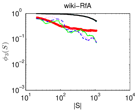
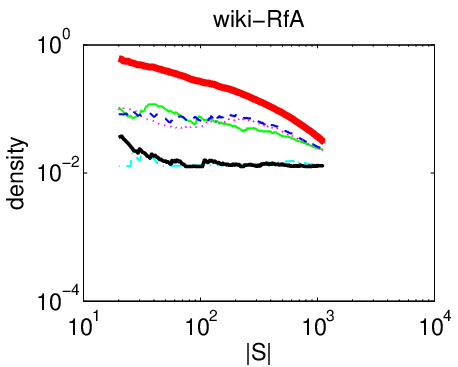
Figure 4 shows the sweep profiles on the networks in Table 1. The results are for a single cut of the network. The plots show the higher-order conductance (Eqn. (3.9)), higher-order expansion (Eqn. (3.10)), and density of the smaller of the partitionined vertex sets. For email-EuAll and wiki-Talk, higher-order conductance is the same for most algorithms, but TSC has much better higher-order expansion when the vertex set gets large enough. On soc-Epinions1 and twitter_combined, standard spectral methods have better higher-order conductance and higher-order expansion. Crucially, in all cases, TSC finds much denser subgraphs. In general, we expect communities with lots of directed 3-cycles to be dense sets. Thus, even though TSC sometimes does not always do well with respect to the score metrics discussed in Sec. 3.4, it is still finding relevant structure.

Since our goal is to explore structural properties of the cuts, we did not tune our TSC algorithms for high performance. Subsequently, we do not compare running times of the algorithms. However, we note that for each network, our straightforward implementation of TSC ran in under 10 minutes using a laptop with 4GB of memory.

References

- [1] N. Alon and V. D. Milman. , isoperimetric inequalities for graphs, and superconcentrators. Journal of Combinatorial Theory, Series B, 38(1):73–88, 1985.
- [2] A. Anandkumar, R. Ge, D. Hsu, S. M. Kakade, and M. Telgarsky. Tensor decompositions for learning latent variable models. arXiv preprint arXiv:1210.7559, 2012.
- [3] P. Boldi, R. Posenato, M. Santini, and S. Vigna. Traps and pitfalls of topic-biased PageRank. In Algorithms and Models for the Web-Graph, pages 107–116. Springer, 2008.
- [4] D. Boley, G. Ranjan, and Z.-L. Zhang. Commute times for a directed graph using an asymmetric Laplacian. Linear Algebra and its Applications, 435(2):224–242, 2011.
- [5] F. Chung. Laplacians and the Cheeger inequality for directed graphs. Annals of Combinatorics, 9(1):1–19, 2005.
- [6] F. R. Chung. Spectral graph theory, volume 92. American Mathematical Soc., 1997.
- [7] J. Cohen. Graph twiddling in a mapreduce world. Computing in Science & Engineering, 11(4):29–41, 2009.
- [8] I. Derényi, G. Palla, and T. Vicsek. Clique percolation in random networks. PRL, 94(16):160202, 2005.
- [9] I. S. Dhillon. Co-clustering documents and words using bipartite spectral graph partitioning. In KDD, 2001.
- [10] N. Durak, A. Pinar, T. G. Kolda, and C. Seshadhri. Degree relations of triangles in real-world networks and graph models. In CIKM, 2012.
- [11] D. F. Gleich. Hierarchical directed spectral graph partitioning, 2006.
- [12] D. F. Gleich, L.-H. Lim, and A. Benson. The Spacey Random Surfer: A stochastic process for multilinear PageRank.
- [13] D. F. Gleich, L.-H. Lim, and Y. Yu. Multilinear PageRank. arXiv, cs.NA:1409.1465, 2014.
- [14] M. S. Granovetter. The strength of weak ties. American Journal of Sociology, pages 1360–1380, 1973.
- [15] C. J. Hillar and L.-H. Lim. Most tensor problems are NP-hard. Journal of the ACM (JACM), 60(6):45, 2013.
- [16] F. Huang, U. Niranjan, M. Hakeem, and A. Anandkumar. Fast detection of overlapping communities via online tensor methods, 2013.
- [17] G. Karypis and V. Kumar. Multilevel k-way hypergraph partitioning. VLSI design, 11(3):285–300, 2000.
- [18] Y. Kim, S.-W. Son, and H. Jeong. Finding communities in directed networks. Phys. Rev. E, 81:016103, Jan 2010.
- [19] C. Klymko, D. F. Gleich, and T. G. Kolda. Using triangles to improve community detection in directed networks. In Proceedings of the ASE BigData Conference, 2014.
- [20] T. G. Kolda and J. R. Mayo. Shifted power method for computing tensor eigenpairs. SIAM Journal on Matrix Analysis and Applications, 32(4):1095–1124, 2011.
- [21] G. Kossinets and D. J. Watts. Empirical analysis of an evolving social network. Science, 311(5757):88–90, 2006.
- [22] E. A. Leicht and M. E. Newman. Community structure in directed networks. PRL, 100(11):118703, 2008.
- [23] J. Leskovec and A. Krevl. SNAP Datasets: Stanford large network dataset collection. http://snap.stanford.edu/data, June 2014.
- [24] Y. Li, Z.-L. Zhang, and J. Bao. Mutual or unrequited love: Identifying stable clusters in social networks with uni-and bi-directional links. In Algorithms and Models for the Web Graph, pages 113–125. Springer, 2012.
- [25] F. D. Malliaros and M. Vazirgiannis. Clustering and community detection in directed networks: A survey. Physics Reports, 533(4):95 – 142, 2013.
- [26] A. Prat-Pérez, D. Dominguez-Sal, J. M. Brunat, and J.-L. Larriba-Pey. Shaping communities out of triangles. In CIKM, 2012.
- [27] L. Qi. Eigenvalues of a real supersymmetric tensor. Journal of Symbolic Computation, 40(6):1302–1324, 2005.
- [28] K. Rohe and B. Yu. Co-clustering for directed graphs; the stochastic co-blockmodel and a spectral algorithm. arXiv preprint arXiv:1204.2296, 2012.
- [29] M. Rosvall, A. V. Esquivel, A. Lancichinetti, J. D. West, and R. Lambiotte. Memory in network flows and its effects on spreading dynamics and community detection. Nature communications, 5, 2014.
- [30] T. Schank and D. Wagner. Finding, counting and listing all triangles in large graphs, an experimental study. In Experimental and Efficient Algorithms. 2005.
9 Proof of Lemma 4.1
Without loss of generality, order the nodes so that the nodes in are first, the nodes are second, and the sink node is last. Let be the transition probabilities of , restricted to nodes in , . Because nodes from two different strongly connected components cannot be in the same directed 3-cycle,
Here, the first block diagonal matrix is of size , the second of size , and the third of size . Consider the following vectors that have the same block structure:
Then , for and . Thus,
The vector satisfies and . Since , is a second left eigenvector. Finally, is positive for all and negative for all .
10 Directed 3-cycle cuts on more networks
Here we present the results of Sec. 6 on more networks. Table 2 lists the statistics of eleven networks that we consider. We include one undirected network, email-Enron. For this data set, all undirected edges are simply replaced with two directed edges. Figures 5, 6, and 7 show the sweep profiles for higher-order conductance, higher-order expansion, and density, respectively.