Collective motion of oscillatory walkers

The movements of all animate things, such as walking of humans, flapping of birds, and swimming of fish, are restricted by their locomotion [1]. Since the collective motion of self-propelled particles (SPP) began to attract interest [2, 3, 4], many studies have been conducted in various contexts [5], including pedestrian crowds [6, 7, 8, 9, 11, 10, 12, 13, 14], bird flocks [15], and insect swarms [16, 17]. However, the effect of locomotion on macroscopic behavior remains an open question. In fact, recent experiments in the field of pedestrian dynamics suggest that the oscillatory motion of pedestrian walking may have a significant effect on overall dynamics [13, 14]. Jelić et al. studied the collective dynamics of pedestrians walking in a line, focusing on bilateral oscillations during walking [13]. From fluctuating trajectories, they obtained the phase of locomotion and investigated the interaction between neighboring pedestrians. Furthermore, Yanagisawa et al. [14] reported that synchronization of the locomotion phase among pedestrians may increase the total flux. Here the “phase” is a mapping from each stage of locomotion to a real number $\phi\in\mathbb{R}/2\pi\mathbb{Z}$. Unlike the situation in the vehicular traffic, this phase is strongly related to the velocity of walkers.

In this paper, we propose a simple model that describes particle-following behavior, phase-velocity coupling, and phase-phase coupling. Particle-following behavior is implemented by the optimal velocity (OV) model [18] for vehicular traffic, which is known to emerge the phase transition from free flow to jam flow that is highly tractable in mathematical analysis. Phase-phase coupling is considered within the framework of the Kuramoto model [19], a paradigmatic model describing synchronization phenomena in nature. In the present study we assume that the phases of successive particles tend to synchronize, which is experimentally suggested when pedestrians walk in a dense crowd [13]. Since each walker follows its predecessor and ignores its successors, the interaction is unidirectional and local. In contrast, other studies have been mainly devoted to globally coupled oscillators or locally but bidirectionally coupled oscillators [20, 21]. Note that we do not consider detailed modeling of actual animals; instead, we concentrate on ideal particles called oscillatory walkers (OWs). Although here we assume the interaction between particles is through their headway distances, it could depend also on their (relative) velocities, which is beyond scope of this paper.

In spite of its simplicity, the OW model presents a rich behavior, including a novel type of jam [Fig. 1(b)]. We report its fundamental characteristic and give insight into collective locomotion.

The rest of the paper is organized as follows: The next section is devoted to define the model. In Sec. III we summarize the dynamics of the model. To understand its destabilization phenomena, theoretical analyses are performed in Sec. IV. Finally we summarize these results in the final section.

Consider $N$ particles, labeled $n=1,\cdots,N$ from left, walking to right on a one-dimensional ring. We impose periodic boundary conditions [particle $(N+1)$ particle is identical to particle $1$]. The velocity of the $n$th walker ($\dot{x}_{n}$) is determined by the following equation:

where $V(\Delta x_{n})$ is the optimal velocity determined for headway distance ($\Delta x_{n}=x_{n+1}-x_{n}$) [18]. Each walker adapts its velocity to this optimal velocity with an adaptation intensity (the reciprocal of the reaction time) $a$. The effect of locomotion is represented by the oscillation term $A(\cos{\phi_{n}}+1)$. The quantity $A$ is the magnitude of the fluctuations in the target velocity, which is set to a small value. The fluctuation phase $\phi_{n}$ is determined by

Here we assume that the ideal angular velocity $\omega(\Delta x_{n})$ is defined by a function similar to the ideal walking velocity $V(\Delta x_{n})$, i.e., using a normalized optimal velocity (NOV) function $U(\Delta x_{n})$, we can express $\omega(\Delta x_{n})=\Omega_{M}U(\Delta x_{n})$ and $V(\Delta x_{n})=V_{M}U(\Delta x_{n})$ . We further impose the condition that when the headway distance is large enough, particles walk with a steady angular velocity $\Omega_{M}U_{\infty}$ and velocity $V_{M}U_{\infty}$, and for small $\Delta x_{n}$, $U(\Delta x_{n})\sim 0$ to stop. To capture these assumptions, the NOV function is set to be a differentiable and monotonically increasing function that is asymptotic to $0$ as $\Delta x_{n}\rightarrow 0$ and to a positive constant as $\Delta x_{n}\rightarrow\infty$. We use the following form of the NOV function when actual calculations are needed: $U(\Delta x_{n})=c_{1}[\tanh(c_{2}\Delta x_{n}-c_{3})+\tanh c_{3}]$ with the positive parameters $c_{1},c_{2}$ and $c_{3}$. $U(\Delta x_{n})$ is a monotonic increasing function such that $U(0)=0$ and $U(\infty)=c_{1}[1+\tanh c_{3}]$. The quantity $c_{3}/c_{2}$ corresponds to its inflection point, and $c_{1}$ and $c_{3}$ determines its height given by $c_{1}[1+\tanh c_{3}]$. Here we set $c_{1}=0.5,c_{2}=5$, and $c_{3}=2.5$.

The second term on the rhs of Eq. (2) represents the synchronous interaction of successive walkers, whose intensity is $K>0$. When the phase difference $\Delta\phi_{n}=\phi_{n+1}-\phi_{n}$ is zero and the walkers are uniformly distributed, they walk with a steady velocity and rhythm (synchronized free flow). In this paper, we restrict the model parameters to $a=3,V_{M}=1,\Omega_{M}=1$ and $N=100$. We vary the particle density $\rho=N/L$ by changing the system length $L$.

The OW model has four types of flow: synchronized free flow (SFF), phase-anchoring free flow (PFF), orderly jam flow (OJF), and disordered jam flow (DJF). “Phase anchoring” occurs when phase differences $\Delta\phi_{n}$ are fixed at a common value, $\Delta\phi_{0}\in(-\pi,\pi]$. When the effects of distance between walkers are negligible, the model reduces to the Kuramoto model with local interactions. Then, the states $\Delta\phi_{n}=$const., in which all angular velocities are identical, are stable over a certain range of $\Delta\phi_{0}$. This property is inherited by the OW model; however, as can be easily verified, the states $\Delta\phi_{n}=$const.$\neq 0$ cannot be realized exactly because of the effects of spatial structure. Actually, each phase difference fluctuates slightly around $\Delta\phi_{0}$ as depicted in Figs. 2(c) and 2(d).

Before going into details, we briefly summarize the dynamics in the system. First, similar to vehicular traffic flow, the model has phase transitions between free flow and (orderly) jam flow; these are caused by increases in the density of walkers. When the density is small ($\rho<\rho_{\rm{cr,1}}$), free flow is stable and a jam cannot develop. At middle densities $\rho_{\rm{cr,1}}<\rho<\rho_{\rm{cr,2}}$, free flow is no longer stable, and small perturbations grow into a jam; this is called OJF [Figs. 1(a) and 2(e)]. At high densities $\rho_{\rm{cr,2}}<\rho$, the system regains stability for free flow. In the free flow regime, the OW model has two types of flow: SFF [Figs. 2(a) and 2(b)] and PFF [Figs. 2(c) and 2(d)]. These flows are locally stable, and all transient flows are asymptotic to either SFF or PFF in the low-density regime, depending on the initial condition. In contrast, in the high-density regime, SFF is always locally stable, while PFF can be destabilized for some parameter regimes, resulting in another type of jam.

In OJF of the middle-density regime, separation of phase differences occurs. As shown in Fig. 2(e), the phase differences become almost constant in each region. This phase anchoring is produced by the spatial structure of OJF, and it also depends on $K$ and the initial conditions.

In addition to these states, another nontrivial phenomenon emerges in the high-density regime, namely disordered jam flow (DJF). This is complex jam flow induced by strong coupling between $\phi_{n}$ and $x_{n}$. As shown in Figs. 1(b) and 2(f), no steady pattern occurs, and small jams propagate with different velocities and even disappear and reappear. The four types of flow correlate with density as in Table. 1.

Now, we investigate the system in detail.

Next, we discuss the stability conditions for each flow. To understand the destabilization of steady free flow, $(x_{n}^{(0)},\phi^{(0)}_{n})$, we investigate how the flow responds to small perturbations. For a small perturbation, $x_{n}=x_{n}^{(0)}+\epsilon_{n},\phi_{n}=\phi_{n}^{(0)}+\delta_{n}$, the system equations (1) and (2) linearize to

with $U^{\prime}(\Delta x^{(0)}_{n})=\frac{\partial U}{\partial\Delta x}|_{\Delta x=\Delta x^{(0)}_{n}}$. When all walkers are uniformly synchronized, namely, $\Delta x_{n}^{(0)}=L/N=1/\rho$, $\phi_{n}^{(0)}=\Omega_{M}U(1/\rho)t\equiv\dot{\phi}_{s}t$, Eqs. (3) and (4) simplify to

Here we assume that $\dot{\phi}_{s}t$ is a fast variable compared to the growth rate of the perturbation, i.e., $\epsilon$, $\delta$, and their derivatives are constant for each period $T=\frac{2\pi}{\dot{\phi}_{s}}$. By integrating Eq. (5) over this period, we can eliminate the vibrational term, leaving

which is the linearized OV model. Now, the stability condition is given by $V_{M}U^{\prime}(1/\rho)<\frac{a}{2}$ [22]. When $\epsilon_{n}$ does not grow in Eq. (7), equation (6) gives the condition on $K$ as $K>0$.

For PFF, the analysis is not straightforward; we start with Eq. (4). By ignoring the coupling between $\epsilon_{n}$ and $\delta_{n}$ as well as the fluctuations in the phase difference (i.e., $\Delta\phi^{(0)}_{n}\simeq\Delta\phi_{0}$), we obtain

From this equation, we can find the stability condition, $|\Delta\phi_{0}|<\frac{\pi}{2}$. Additionally, since the system is periodic ($\phi_{N+1}=\phi_{1}$), the condition $N\Delta\phi_{0}=2m\pi\quad(m=\pm 1,\pm 2,\cdots)$ must be satisfied. To summarize, stable $\Delta\phi_{0}$ can take the discrete values of $\Delta\phi_{0}=0,\pm\frac{2\pi}{N},\pm\frac{4\pi}{N},\cdots,\pm\left(\frac{\lfloor N/2\rfloor-2}{N}\right)\pi$, where $\lfloor Y\rfloor$ is the floor function giving the maximum integer not larger than $Y$. These conditions were verified by numerical simulations. On the other hand, the coupling behavior of $\epsilon_{n}$ and $\delta_{n}$ is determined by the final term in Eq. (3). If the time integral $\int_{0}^{T^{\prime}}{\sin{\phi^{(0)}_{n}}dt}\neq 0$ (i.e., if the sine function is “distorted”), the system can destabilize. This distortion is also observed as a change of flux in the high-density regime (Fig. 3. See also approximate analyses in Appendix B.). From these facts, we conclude that the high-density regime leads to coupling in the stability equation, which may result in DJF.

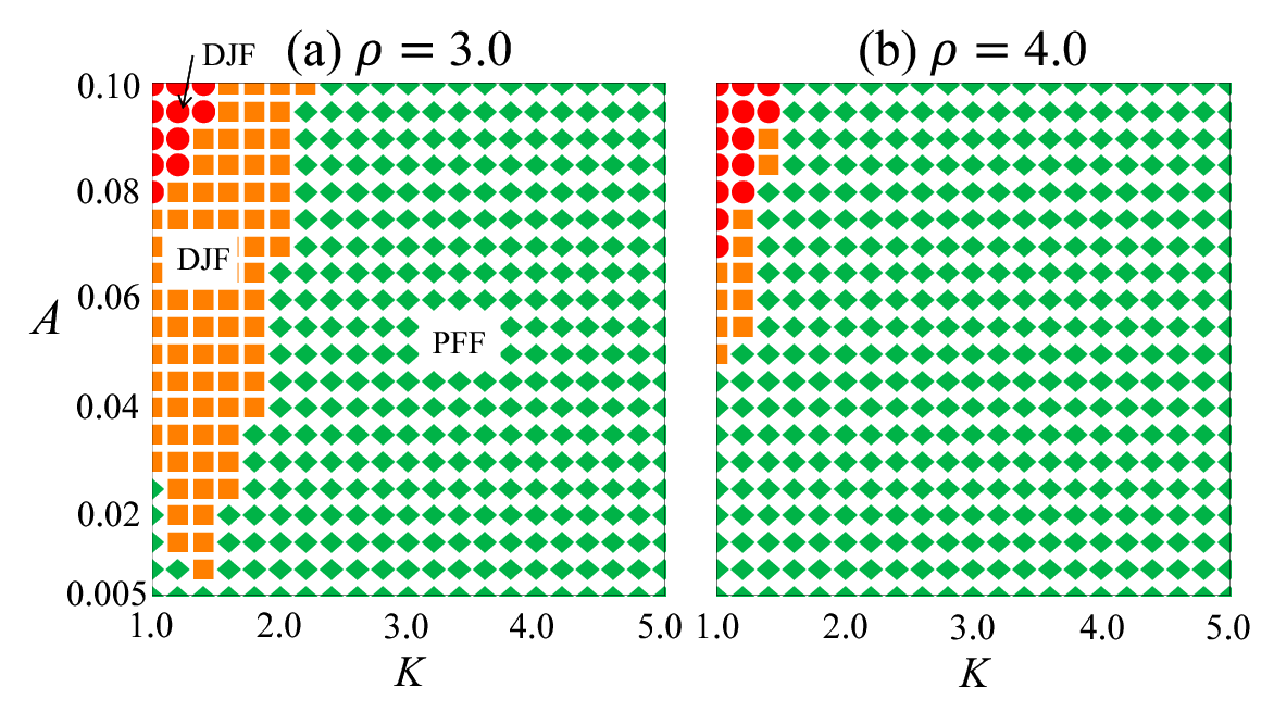
In Fig. 5 we illustrate the phase diagrams of the system by simulations, using the expression for PFF $(x_{n,1},\phi_{n,1})$ (whose derivation is found in Appendix A) as initial conditions, to see whether the flow is stable or not:

where $v_{0}=V(1/\rho)+A,\dot{\phi}_{0}=\omega(1/\rho)+K\sin{\Delta\phi_{0}},\varphi_{0}=\tan^{-1}(\dot{\phi}_{0}/a)$, and $\Psi(t)=\dot{\phi}_{0}t-\varphi_{0}+\Delta\phi_{0}n$. It is found that the system destabilizes for small $K$ and large $A$, and for especially large values of $A$, particles even collide with each other in DJF. Thus we can conclude that the increase of $A$ and $K$ are connected to the destabilization and stabilization of the system, respectively. In addition, increase of particle density reduces the DJF regime, because it decreases space for “over acceleration” of particles that is indispensable for DJF.

In summary, we have proposed a simple model to show that the restriction coming from locomotion largely affects the collective behavior of SPPs. The model has various types of flow, including a novel type of complex flow called disordered jam flow (DJF). Disordered jam flow appears when the particle density is high; this flow is caused by coupling between velocities and phases of particles. We also find that particle flux is strongly affected by phase anchoring. On the other hand, some issues remain to be clarified in future studies. These include, synchronization phenomena on inhomogeneous distributions of intrinsic optimal velocity and angular velocity, quantitative analysis for phase anchoring and its effect on flux, etc. These points should be addressed in detail in future works.

Although pedestrian locomotion in a crowd is not yet fully understood, a real pedestrian may adapt the crowd velocity and step length by considering the environment of other pedestrians (not only the nearest predecessor). Furthermore, the environment may affect a pedestrian through a strong psychological repulsive force [11]. We believe that by including the effects of phase, models for pedestrians and other animals can be improved. Moreover, the synchronization of pedestrians through a bridge [23, 24] might be an interesting problem. It is also attractive to extend this model to two dimensions using the two-dimensional OV model [25], which generalization would require additional rules of phase synchronization.

We thank Hiroshi Kori for his insightful comments on this study.

References

- [1] M. R. Alexander, Locomotion of animals (Blackie and Son, Glasgow, 1982).
- [2] T. Vicsek, A. Czirok, E. Ben-Jacob, I. Cohen, and O. Shochet, Phys. Rev. Lett. 75, 1226 (1995).
- [3] J. Toner and Y. H. Tu, Phys. Rev. Lett. 75, 4326 (1995).
- [4] J. Toner and Y. H. Tu, Phys. Rev. E 58, 4828 (1998).
- [5] T. Vicsek and A. Zafeiris, Phys. Rep. 517, 71 (2012).
- [6] D. Helbing, I. Farkas, and T. Vicsek, Nature (London) 407, 487 (2000).
- [7] D. Helbing, Rev. Mod. Phys. 73, 1067 (2001).
- [8] A. Schadschneider, D. Chowdhury, K. Nishinari, Stochastic Transport in Complex Systems: From Molecules to Vehicles (Elsevier Science, Amsterdam, 2010).
- [9] M. Chraibi, A. Seyfried, and A. Schadschneider, Phys. Rev. E 82, 046111 (2010).
- [10] C. Burstedde, K. Klauck. A. Schadschneider, and Zittartsz, Physica A 207, 507 (2001).
- [11] T. Ezaki, D. Yanagisawa, K. Ohtsuka and K. Nishinari, Physica A 391, 291 (2012).
- [12] T. Ezaki, D. Yanagisawa, K. Nishinari, Phys. Rev. E 86, 026118 (2012).
- [13] A. Jelić, C. Appert-Rolland, S. Lemercier, and J. Pettré, Phys. Rev. E 86, 046111 (2012).
- [14] D. Yanagisawa, A. Tomoeda, and K. Nishinari, Phys. Rev. E 85, 016111 (2012).
- [15] K. Bhattacharya and T. Vicsek, New J. Phys. 12, 093019 (2010).
- [16] P. Romanczuk, I. D. Couzin, and L. Schimansky-Geier, Phys. Rev. Lett. 102, 010602 (2009).
- [17] K. Nishinari, D. Chowdhury and A. Schadschneider, Phys. Rev. E 67, 036120 (2003).
- [18] M. Bando, K. Hasebe, A. Nakayama, A. Shibata, and Y. Sugiyama, Phys. Rev. E 51, 1035 (1995).
- [19] Y. Kuramoto, Chemical Oscillations, Waves and Turbulence (Springer-Verlag, Berlin, 1984).
- [20] A. H. Cohen, P. J. Holmes, and R. H. Rand, J. Math. Biol. 13, 345 (1982).
- [21] J. A. Acerbrón, L. L. Bonilla, C. J. Pérez-Vicente, F. Ritort, and R. Spigler, Rev. Mod. Phys. 77, 137 (2005).
- [22] We can obtain this condition by substituting the expansions and , and putting . See also Ref. [18].
- [23] S. H. Strogatz, D. M. Abrams, A. McRobie, B. Eckhardt, and E. Ott, Nature (London) 438, 43 (2005).
- [24] B. Eckhardt, E. Ott, S. H. Strogatz, D. M. Abrams, and A. McRobie, Phys. Rev. E 75, 021110 (2007).
- [25] A. Nakayama, K. Hasebe, and Y. Sugiyama, Phys. Rev. E 71, 036121 (2005).