A weighted minimum gradient problem with complete electrode model boundary conditions for conductivity imagingThanks: Received by the editors 2015.
Abstract
We consider the inverse problem of recovering an isotropic electrical conductivity from interior knowledge of the magnitude of one current density field generated by applying current on a set of electrodes. The required interior data can be obtained by means of MRI measurements. On the boundary we only require knowledge of the electrodes, their impedances, and the corresponding average input currents. From the mathematical point of view, this practical question leads us to consider a new weighted minimum gradient problem for functions satisfying the boundary conditions coming from the Complete Electrode Model (CEM) of Somersalo, Cheney and Isaacson. We show that this variational problem has non-unique solutions. The surprising discovery is that the physical data is still sufficient to determine the geometry of (the connected components of) the level sets of the minimizers. We thus obtain an interesting phase retrieval result: knowledge of the input current at the boundary allows determination of the full current vector field from its magnitude. We characterize locally the non-uniqueness in the variational problem. In two and three dimensions we also show that additional measurements of the voltage potential along a curve joining the electrodes yield unique determination of the conductivity. The proofs involve a maximum principle and a new regularity up to the boundary result for the CEM boundary conditions. A nonlinear algorithm is proposed and implemented to illustrate the theoretical results.
keywords
minimum gradient, conductivity imaging, complete electrode model, current density impedance imaging, minimal surfaces, magnetic resonance electrical impedance tomography, current density impedance imagingAMS
35R30, 35J60, 31A25, 62P101 Introduction
We consider the inverse problem of reconstructing an inhomogenuous isotropic electrical conductivity in a domain , , from interior knowledge of the magnitude of one current density field and of corresponding boundary data.
Most of the existing results on this problem (see a brief survey of previous work at the end of this introduction) consider Dirichlet boundary conditions. In this paper we study boundary conditions which model what can actually be measured in practical experiments. We work with the beautiful Complete Electrode Model (CEM) originally introduced in [28] and shown to best describe the physical data: For , let denote the surface electrode of constant impedance through which one injects a net current .
The CEM assumes the voltage potential inside and the constant voltages ’s on the surface of the electrodes distribute according to the boundary value problem
| (1) | ||||
| (2) | ||||
| (3) | ||||
| (4) |
where is the outer unit normal. If a solution exists, an integration of (1) over together with (3) and (4) show that
| (5) |
is necessary. Physically, the zero sum of the boundary currents account for the absence of sources/sinks of charges. The constants appearing in (2) represent unknown voltages on the surface of the electrodes, and the difference from the traces of the interior voltage potential governs the flux of the current through the skin to the electrode. We refer to the problem (1), (2), (3), and (4) as the forward problem.
Under the assumptions that is a Lipschitz domain, the conductivity is essentially bounded with real part bounded away from zero, the electrodes are (relatively) open connected subsets of whose closure are disjoint, the impedances have positive real part, and the injected currents satisfy (5), the forward problem has a unique solution up to an additive constant, as shown in [28]. We normalize this constant by imposing the electrode voltages to lie in the hyperplane
| (6) |
The net input currents , as in (5), generate a current density field , where is the solution of the forward problem.
In this paper we consider the inverse problem of determining , given the magnitude
| (7) |
of the current density field inside .
The conductivity is unknown but assumed real valued and satisfying
| (8) |
Each electrode , is a known Lipschitz domain subset of the boundary. The surface impedances are assumed real valued. In general we allow them to be inhomogenous functions on the electrodes satisfying
| (9) |
Further smoothness conditions will be assumed for some of the results in this paper.
We note that, in practice, interior measurements of all three components of the current density can be obtained from three magnetic resonance scans involving two rotations of the object [27]. However recent engineering advances in ultra-low field magnetic resonance may be used to recover without rotating the object [26]. We hope that the results presented here may lead to further experimental progress on easier ways to measure directly just the magnitude of the current.
We start by remarking that there is non-uniqueness in the inverse problem stated above, as can be seen in the following example: Let be the unit square. We inject the current through the top electrode of impedance , “extract” the current through the bottom electrode of impedance , and measure the magnitude of the current density field in . Then, for every an increasing Lipschitz continuous function, satisfying , the function solves the forward problem (1), (2), (3), and (4) corresponding to a conductivity , yet the magnitudes of the corresponding current densities yield the same interior measurements .
More generally, if is the solution of the forward problem for some , let be any Lipschitz-continuous increasing function of one variable, such that whenever , for each , and constants satisfying . One can easily verify that the function
| (10) |
solves the forward problem with the conductivity
| (11) |
while .
For Hölder-continuous conductivities, in Theorem 2 we prove that (10), (11) must hold in a neighborhood of any non-critical point. The following example shows that (10), (11) need not hold in the whole domain for a single function .
Let be the curvilinear octagon with hyperbolic sides obtained from the unit disc, by carving out the peripheral regions along the branches of the hyperbolas , and . The electrodes are defined respectively by each connected component of inside the disc, whereas are defined respectively by the connected components of . Thus defined, all the electrodes have equal length, denoted by . We assume constant impedances . Through and one inputs the net currents , and extracts through and . In one measures . It is easy to check that the constant conductivity is a possible solution to the inverse problem, with the corresponding voltage . However, this is not the only possibility: Let
and be any two increasing Lipschitz continuous functions with in , for some sufficiently small. Define a new conductivity by
| (12) |
As in the previous examples, one can check that is also a solution of the inverse problem for the same , with corresponding potential equal to on , and equal to on , respectively.
Similar to the approach in [22], we formulate the inverse problem in terms of a weighted minimum gradient problem. Here we need a functional which is appropriate for the boundary conditions coming from the Complete Electrode Model and is entirely defined in terms of the data in the inverse problem. To obtain such a functional, we found it necessary to revisit the forward problem and recast it as a minimization problem, see Appendix A. We are then able to show that the solution of the forward problem is a global minimizer of the functional
| (13) |
over , with as in (7).
Using , we found the surprising fact that, given the positions and impedances of the electrodes, knowledge of the magnitude of one current density field and of the corresponding average applied currents (just one number in the case of two electrodes!) is still sufficient to determine the geometry of the connected components of the equipotential sets. Furthermore, we remark that, since we recover the direction (including orientation) of the electric field , we also obtain an interesting phase retrieval result: the full current density vector field is recovered from its magnitude , and knowledge of the input currents on the surface electrodes, even though the conductivity is not uniquely determined.
Uniqueness of the conductivity can be restored by additional measurement of the voltage potential on a curve connecting the electrodes; see Theorem 6. The additional measurement involves only a one dimensional subset of boundary measurements, much less than required in the existing results for the Dirichlet problem.
For the unique determination result we assume that the curve and the set of electrodes satisfy a topological assumption, see (30).
To illustrate the theoretical results, we propose an iterative algorithm and perform a numerical experiment, see Section 5. Similar to the algorithm in [22] we decrease the functional on a sequence of solutions of forward problems for updated conductivities.
Conductivity imaging using the interior knowledge of the magnitude of current densities was first introduced in [12]. The examples of non-existence and non-uniqueness for the ensuing Neumann problem lead the authors of [12] to consider the magnitudes of two currents. The possibility of conductivity imaging via the magnitude of just one current density field was shown in [21] via the Cauchy problem, and in [22, 24] via a minimum gradient problem with Dirichlet boundary conditions. Existence and uniqueness of such weighted gradient problems was studied in [8]. Extensions to the case of inclusions with zero or infinite conductivity were obtained in [19, 20]. A structural stability result for the minimization problem can be found in [25]. Reconstruction algorithms based on the minimization problem were proposed in [22] and [18], and based on level set methods in [21, 22, 30]. A local Hölder- continuous dependence of on (for unperturbed Dirichlet data) has been recently established in [17]. For further references on determining the isotropic conductivity based on measurements of current densities see [32, 12, 14, 15, 11, 16, 13], and for some results on anisotropic conductivities see [10, 7, 1, 2].
2 A weighted minimum gradient problem for the CEM boundary conditions
In this section we show that the solution of the forward problem is a global minimizer of the functional in (13) over . The regularity assumptions are the ones from the forward problem.
Proposition 1.
Proof.
For any , we have the inequality
| (15) |
where the first equality uses (7), the next line uses (3) and the Cauchy-Schwarz inequality, the next equality uses (1) and the divergence theorem, the third equality uses (4), and the last equality uses (2).
In particular, when , the inequality in the estimate (15) holds with equality yielding
| (16) |
and
| (17) |
The global minimizing property (14) then follows from (15) and (17) using the pointwise inequality
| (18) |
∎
3 Local characterization of non-uniqueness and applications
In this section we state and prove our main result and its consequences to the conductivity imaging problem.
Theorem 2.
Let , be a bounded, Lipschitz domain, and let , , be disjoint subsets of the boundary of positive surface measure. Assume that the corresponding impedances satisfy (9), and that the given currents are such that (5) holds. Let , be the solutions of the forward problem (1), (2), (3), and (4) corresponding to unknown conductivities satisfying (8). Assume that
| (19) |
Then:
(i) for each ,
| (20) |
Proof.
From the interior elliptic regularity we have ; see, e.g., [4, Theorem 8.34]. Thus, the sets of critical points of and are closed, and, by hypothesis (19) they are negligible. Let denote their union. It follows that is open and dense in .
According to Proposition 1 and are both minimizers of , and thus
| (23) |
In particular, using (17), (23), (15), and (18), the inequalities
must be equalities. Thus,
| (24) |
We will prove part (ii) for any point in .
Since (15) holds with equality, we must also have
| (25) |
Since both gradients are continuous, in view of (25) they must be parallel whenever one of them is nonzero, in particular
| (26) |
for some with in . Moreover, since is dense, extends by continuity to the whole domain .
Let be arbitrarily fixed. For some component , . Consider defined by if , and . Then the Jacobian determinant
and, by the inverse function theorem, there is a neighborhood of in , such that is a diffeomorphism.
Consider . We use (26) to show that
is independent of , for all . Indeed, for ,
where the second equality uses (26) and the next to the last equality uses the definition of .
For each we can now well define
| (27) |
If , then , and the equation above shows
Finally, since and are constant on each other’s connected components of level sets within (as can be seen from a differentiation in the direction tangential to the level set and (26)), the identity (21) extends to points on any connected component of a level set of passing through .
∎
The result above implies that knowledge of the input currents at the boundary is sufficient to determine the full current density from measurements of its magnitude in the interior, even when the conductivity is not determined uniquely. Thus we have obtained the following “phase retrieval” result, which may be of independent interest.
Corollary 3 (Phase retrieval).
Let , be a bounded, Lipschitz domain, and let , , be disjoint subsets of the boundary of positive surface measure. Assume that the corresponding impedances satisfy (9), and that the given currents are such that (5) holds. Let be the solutions of the forward problem (1), (2), (3), and (4) corresponding to unknown conductivities satisfying (8). Let and be the corresponding current densities. If
| (28) |
then
| (29) |
4 Unique determination for two and three dimensional models
To determine the conductivity uniquely, we will assume additional knowledge of the voltage potential on some part of the boundary. For brevity, let denote the set of all electrodes.
We show below that knowledge of the voltage potential along a boundary curve which joins the electrodes is sufficient to yield uniqueness in two and three dimensional domains. We assume that satisfies the topological assumption:
| (30) |
In two dimensions the second assumption is trivially satisfied.
For the proof of the uniqueness result we need continuity of solutions up to the boundary for -harmonic functions satisfying CEM boundary conditions.
As a direct consequence of the Proposition 12 and the Sobolev embedding theorem we have the following.
Corollary 4.
Let be a -domain, , and let be -smooth near the boundary. Assume that the electrodes has Lipschitz boundaries, and , . Let be the solution to the forward problem. Then
a) , for .
b) For any , there is a neighborhood of , such that , for .
Another idea in the uniqueness result below is that the range of on the union of the curve and the electrodes is the same as the range of in . This follows from the following maximum principle for the CEM, which may be of independent interest.
Proposition 5.
(Maximum principle for CEM) Under the smoothness assumptions in the Corollary 4, the solution achieves its minimum and maximum on . If is a curve such that is connected, then the range of over coincides with the range of over .
Proof.
By the weak maximum principle, the maximum and minimum of over occur on the boundary. By Hopf’s strong maximum principle, at a point of maximum, say , the normal derivative must be strictly positive. From the boundary condition (4) we then deduce . The same argument applies to a point of minimum, where the normal derivative is strictly negative. Since is connected, and is continuous on , is a closed interval. Since the maximum and minimum occur on , then the range .
∎
We are now ready to prove our main uniqueness result.
Theorem 6 (Unique determination).
Let be a -domain, . Assume that the electrodes have Lipschitz boundaries, and , . For the currents satisfying (5), let be the solutions of the forward problem (1), (2), (3) and (4) corresponding to unknown conductivities , which are assumed -smooth near the boundary and satisfying (8).
If
| (31) | ||||
| (32) |
then
| (33) | ||||
| (34) |
Proof.
We will give the proof for the three dimensional case and indicate where arguments simplify in the two dimensional case.
From Corollary 4 we know that and are continuous up to the boundary. In particular, the identity (20) in Theorem 2 shows that on each electrode , . Since on by hypothesis (32), we conclude that for each . So far we showed that and coincide on , and following Proposition 5, .
We refer to a value as being regular if the corresponding -level set is free of singular points. For -regular, let be a connected component of the - level set. The arguments in [22, Theorem 1.3] showing that reaches do not use any boundary information, and thus they remain valid for the CEM boundary conditions; we recall them in Appendix B for completeness.
To prove unique determination, it now suffices to show that intersects . We reason by contradiction: Assume that misses . Then the intersection is entirely contained in a connected component . By hypothesis (30) is simply connected. Moreover, as transversal (in fact orthogonal) intersection of -smooth surfaces, the set is a one dimensional immersed - submanifold without boundary, i.e. a closed curve (in two dimensions it consists of two points). Since has no singular points, the curve has no self-intersection and thus is a simple closed curve embedded in the simply connected subset . By the Jordan curve theorem, separates in two parts, one of which, say , is enclosed by . Let be the subset of whose boundary is , and define the new function
| (35) |
Note that may have modified values at the boundary, but only off the electrodes. Since is an extension domain ( has a unit normal everywhere) the new map and strictly decreases the functional (13) unless . This contradicts the minimizing property of . Therefore in , which now contradicts (31). Therefore intersects , and thus . Since the set is dense in , the identity (33) follows. Now (31) yields that , a.e. in , and by continuity in .
∎
5 A minimization algorithm for the weighted gradient functional with CEM boundary constraints
In this section we propose an iterative algorithm which minimizes the functional in (13). It is the analogue of an algorithm in [22] adapted to the CEM boundary conditions.
The following lemma is key to constructing a minimizing sequence for the functional .
Lemma 7.
Assume that satisfies
| (36) |
for some , and let be the unique solution to the forward problem for . Then
| (37) |
Moreover, if equality holds in (37) then .
Proof.
Let be arbitrary. Since is a global minimizer of as in (58) with as shown in Theorem 11, we have the inequality:
| (38) |
Writing
we also obtain
| (39) |
From (38) and (39) we conclude (37). Moreover, if the equality holds in (37) then equality holds in (38), and thus
| (40) |
Since is a solution to the forward problem (for ) it is also a global minimizer of over . But (40) shows that is also a global minimizer for . Now the uniqueness of the global minimizers in Theorem 11 (for ) yields .
∎
Algorithm: We assume the magnitude of the current density satisfies
| (41) |
Let be the lower bound in (8), and a measure of error to be used in the stopping criteria.
6 Numerical Implementations
We illustrate the theoretical results on a numerical simulation in two dimensions.
6.1 An algorithm for the forward problem
Given a current pattern and a set of surface electrodes with impedances (taken to be constant)for satisfying (9), our iterative algorithm consists in solving the forward problem (1), (2), (3)and (4) for an updated conductivity at each step.
A piecewise linear (spline) approximation of the solution to the forward problem is sought on an uniform triangulation of the unit box as shown in figure 1.
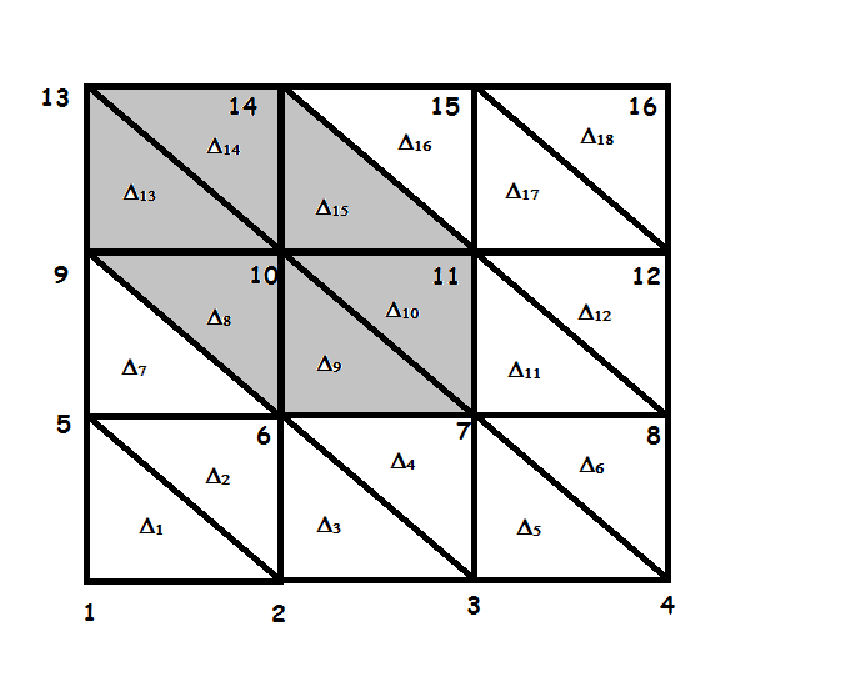
For a (square) number of grid nodes, let be the set of planes supported in the -th triangle , for . More precisely, when ,
where is the southwest grid point of the square in which is inscribed, and is the length of the side of the square.
When ,
where is the northeast grid point of the square in which is inscribed, and is the length of the side of the square. For example, in Figure 1 the triangle lies in a square whose southwest grid point position is and the northeast grid point location is .
We seek an approximation to the solution of the forward problem (1), (2), (3), and (4) in the form
| (43) |
where is the sum over those planes ’s, that are adjacent to the -th node in the unit box, see figure 1. By substituting (43) into (59), and by selecting , for , and , we get the set of equations
| (44) |
which is augmented with the second set of equations
| (45) |
obtained by setting and whenever for , and for .
Note that forming in this fashion is equivalent to choosing for each the -th vector for the -th equation in (45) from the set
which is a basis for , and then setting
The values of are then solutions to the linear system
| (46) |
where the entries of are
the entries of are
and
In the matrix above denotes the surface area of the electrode, for .
For other numerical schemes for solving the forward problem we refer to [31].
6.2 Simulating the interior data
We consider a simulated planar conductivity (which models the cross section of a torso) embedded in the unit box ; see Figure 2 on the left. The values of the conductivity range from to .
Two currents are respectively injected/extracted through the electrodes
of equal impedances .
6.3 Numerical reconstruction of a simulated conductivity
Knowing the injected currents and , the electrode impedances and , and the corresponding magnitude of the current density we find an approximate minimizer of via the iterative algorithm in section 5. The iterations start with the guess . An approximate solution is computed on a grid. The stopping criterion (42) for this experiment used , and was attained with 320 iterations. An intermediate conductivity is computed using the computed minimizer , see Figure 3.

We note that in this example everywhere, thus all the level sets of are connected. It follows from the arguments in Section 3 that there is a unique such that and
The function can be determined from knowledge of on the curve , which connects the two electrodes. More precisely, for each point on the function maps the computed value of to the measured value of at the same point. Figure 4 on the left shows the resulting on the range . Figure 4 on the right shows , which is the scaling factor needed to obtain the true conductivity .

In Figure 5 the reconstructed conductivity is shown on the right against the exact conductivity on the left. The error of the reconstruction is .
Acknowledgments
We are grateful to the anonymous referees for their valuable comments. In particular one of the comments uncovered a gap in a previous version of the manuscript, and another comment suggested that our arguments would also work for the Neumann problem (see the remark at the end of Section 3). The work of A. Tamasan has been supported by the NSF Grant DMS-1312883, as was that of J. Veras as part of his Ph.D. research at the University of Central Florida. The work of A. Nachman has been supported by the NSERC Discovery Grant 250240.
Appendix A A minimization approach for the Complete Electrode Model
In this appendix we show solvability of the forward problem for the Complete Electrode Model of [28] by recasting it into a minimization problem. While this approach is less general than the one given in [28] (we assume a real valued conductivity and positive electrode impedances), it explains how we are led to introduce the functional (13) in the solution of the inverse problem. For existence and uniqueness of solutions of the forward problem, the conductivity and electrode impedances need not be smooth: and satisfy
| (47) |
Let be the space of functions which together with their gradients lie in , and be the hyperplane in (6). We seek weak solutions to (1), (2) (3), (4), and (5) in the Hilbert space , endowed with the product
and the induced norm
| (48) |
We’ll need the following variant of the Poicaré inequality, suitable for the complete electrode model.
Proposition 8.
Let , , be an open, connected, bounded domain with Lipschitz boundary , and be the hyperplane in (6). For , let be disjoint subsets of the boundary of positive induced surface measure: .
There exists a constant , dependent only on and the ’s, such that for all and all , we have
| (49) |
Proof.
We will show that
| (50) |
We reason by contradiction: Assume the infimum in (50) is zero. Without loss of generality (else normalize to 1), there exists a sequence in the unit sphere of , , and such that
| (51) | ||||
| (52) |
Due to the compactness of the unit sphere in and of the weakly compactness of the unit sphere in it follows that there exists some with
| (53) |
such that, on a subsequence (relabeled for simplicity),
| (54) | ||||
| (55) |
Since the sequence is bounded in , the trace theorem implies that is (uniformly in ) bounded in , hence also in , for each . Using (52) and (55) in
we obtain . Since , we conclude that
| (56) |
From (56) and (57) we conclude that restricts to the same constant on each electrode, and thus Since , we must have and then , thus contradicting (53).
∎
Proposition 9.
Let , , and , be as in Proposition 8. For , and , satisfying (47), and , let us consider the quadratic functional defined by
| (58) |
Then
(i) is strictly convex
Proof.
(i) The functional has two quadratic terms, each strictly convex, and one linear term, hence the sum is strictly convex. (ii) The Gateaux differentiability and the formula (59) follow directly from the definition of .
The proposition below revisits [28, Proposition 3.1.] and separates the role of the conservation of charge condition (5). This becomes important in our minimization approach, where we shall see that has a unique minimizer independently of the condition of (5) being satisfied. However, it is only for currents satisfying (5), that the minimizer satisfies (3). This result does not use the reality of and of ’s. Recall that the Gateaux derivative of is given in (59).
Proposition 10.
Let , , , , , and be as in Proposition 9.
Proof.
(i) Follows from a direct calculation and Green’s formula.
(ii) Assume that (61) holds.
For each fixed keep as above, but now choose arbitrary with . A straightforward calculation starting from (61) shows that
Since were arbitrary (2) follows.
Now choose as above but arbitrary with for all . It follows from (61) that
Since the trace of is arbitrary off the electrodes (4) holds.
Finally, for an arbitrary choose with the trace on each , and off the electrodes. By using the already established relations (1), (2), (4) and Green’s formula in (61) we obtain
On the one hand, by introducing the notation with
we just showed that . Note that so far we have not used the conservation of charge condition (5).
On the other hand, by using (4), (5), and (1) in the divergence formula, we have
which yields . Therefore , and (3) holds.
∎
The following result establishes existence and uniqueness of the weak solution to the foward CEM problem; contrast with the proof of Theorem 3.3 in [28].
Theorem 11.
Proof.
(i) Let
and consider a minimizing sequence in ,
| (62) |
Since we have . Following (60),
Thus the minimizing sequence must be bounded, hence weakly compact. In particular, for a subsequence (relabeled for simplicity) there is some , such that
| (63) |
On the other hand since is convex, and Gateaux differentiable at in the direction , we have
| (64) |
We take the limit as . The weak convergence in (63) yields
Thus which shows that is a global minimizer. Strict convexity of implies it is unique. At the minimum the Euler-Lagrange equations (61) are satisfied. An application of Proposition 10 part (ii) shows that is a weak solution to the forward problem.
(ii) Proposition 10 part (i) shows that solves the Euler-Lagrange equations, and due to the convexity it is a minimizer of . Due to the strict convexity of the functional the minimizer is unique, hence the weak solution is unique.
∎
Appendix B On the regularity up to the boundary for CEM boundary conditions
If , then interior elliptic regularity yields . The following result considers the regularity up to the boundary; part a) in the proposition below was already proved in [3, Remark 1]. We reproduce the proof for the reader’s convenience. Let be the union set of the electrodes.
Proposition 12.
Let be a -domain, and let be -smooth near the boundary. Assume that the electrodes has Lipschitz boundary, and , . Let be the solution to the forward problem.
Then
a) , for all .
b) For any , there is a neighborhood of , and a function for all , such that .
Proof.
a) Since it follows from (2) that . Since , we have . By [9, Theorem 11.4] the extension by zero to the whole boundary yields , and thus . Now apply the elliptic regularity for the Neumann problem [9, Remark 7.2] to conclude , for all .
b) Let , and choose be sufficiently small so that is -smooth in and .
Let . We define
where is the cutoff function with , if , and if . Then, by part a) we have
for all .
Also by part a) we have that the trace . Now, by (2),
and thus, Now apply the elliptic regularity [9, Theorem 7.4, Remark 7.2] to conclude .
If , the same proof holds if we choose such that . ∎
Appendix C The connected components of almost all level sets reach the boundary
Let be one of the values for which the level set is a - smooth hypersurface (which is the case for a.e. ), and be one of its connected components. We show here that . The arguments in the proof of [22, Theorem 1.3] use only the interior points of , and thus apply to the CEM as well. We include them here for the convenience of the reader.
Arguing by contradiction, assume that . Then is a compact manifold with two connected components. Using the Alexander duality theorem in algebraic topology for (see, e.g. Theorem 27.10 in [5],) we have that is partitioned into three open connected components: . Since we have and then for .
We claim that at least one of the or is in . Assume not, i.e. for each , . Since is connected (by assumption), we have that is connected which implies is also connected. By applying once again Alexander’s duality theorem for , we have that has exactly two open connected components, one of which is unbounded: . Since is connected and unbounded, we have , which leaves . This is impossible since is open and is a hypersurface. Therefore either or or both has the boundary in .
To fix ideas, consider . If this were the case, then we claim that in . Indeed, since is an extension domain ( has a unit normal everywhere) the new map defined by
is in and decreases the functional (13), thus contradicting the minimizing property of . Therefore in , which makes in . Again we reach a contradiction since the set of critical points of is negligible.
These contradictions followed from the assumption that , and therefore
References
- [1] G. Bal, C. Guo and F. Monard, Imaging of anisotropic conductivities from current densities in two dimensions, SIAM J. Imag. Sci. 7(4), (2014), 2538–2557.
- [2] G. Bal, C. Guo and F. Monard, Inverse anisotropic conductivity from internal current densities Inverse Problems 30 (2), (2014), 025001
- [3] J. Dardé, H. Hakula, N. Hyvönen, and S. Staboulis, Fine-tuning electrode information in electrical impedance tomography, Inverse Problems Imaging 6(2012), 399 - 421.
- [4] D. Gilbarg and N. S. Trudinger, Elliptic Partial Differential Equations, 2nd ed., Springer-Verlag, NY, 2001.
- [5] J. M. Greenberg and J. R. Harper, Algebraic Topology, Benjamin - Cummings, 1981.
- [6] M. Hanke, B. Harrach, and N. Hyvönen, Justification of point electrode models in electrical impedance tomography, Math. Models Methods Appl. Sci. 21(6), 2011, 1395-141
- [7] N. Hoell, A. Moradifam, and A. Nachman, Current Density Impedance Imaging with an Anisotropic Conductivity in a Known Conformal Class, SIAM J. Math. Anal. 46 (2014), 3969–3990.
- [8] R. L. Jerrard, A. Moradifam, and A. Nachman, Existence and uniqueness of minimizers of general least gradient problems, J. Reine Angew. Math., to appear.
- [9] J.-L. Lions and E. Magenes, Non-homogeneous Boundary Value Problems and Applications, Vol. I, Springer, Berlin, 1972.
- [10] W. Ma, T. P. DeMonte, A. I. Nachman, N. M. H. Elsaid and M. L. G. Joy, Experimental Implementation of a New Method of Imaging Anisotropic Electric Conductivities, EMBC, Osaka, (2013), 6437 - 6440.
- [11] M. J. Joy, A. I. Nachman, K. F. Hasanov, R. S. Yoon, and A. W. Ma, A new approach to Current Density Impedance Imaging (CDII), Proceedings ISMRM, No. 356, Kyoto, Japan, 2004.
- [12] S. Kim, O. Kwon, J. K. Seo, and J. R. Yoon, On a nonlinear partial differential equation arising in magnetic resonance electrical impedance tomography, SIAM J. Math. Anal., 34 (2002), pp. 511–526.
- [13] Y-J Kim and M-G Lee, Well-posedness of the conductivity reconstruction with interior data and virtual resitive networks, Preprint 2014
- [14] O. Kwon, E. J. Woo, J. R. Yoon, and J. K. Seo, Magnetic resonance electric impedance tomography (MREIT): Simulation study of J-substitution algorithm, IEEE Trans. Biomed. Eng., 49 (2002), pp. 160–167
- [15] O. Kwon, J. Y Lee, and J. R. Yoon, Equipotential line method for magnetic resonance electrical impedance tomography, Inverse Problems. 18 (2002), pp. 1089-�1100
- [16] J. Y. Lee A reconstruction formula and uniqueness of conductivity in MREIT using two internal current distributions, Inverse Problems, 20 (2004), pp. 847–858
- [17] C. Montalto and P. Stefanov, Stability of coupled physics inverse problems with one internal measurement, Inverse Problems, 29(2013), no. 12, 125004.
- [18] A. Moradifam, A. Nachman, and A. Timonov, A convergent algorithm for the hybrid problem of reconstructing conductivity from minimal interior data, Inverse Problems, 28 (2012) 084003.
- [19] A. Moradifam, A. Nachman, and A. Tamasan, Conductivity imaging from one interior measurement in the presence of perfectly conducting and insulating inclusions, SIAM J. Math. Anal., 44(2012) (6), 3969-3990.
- [20] A. Moradifam, A. Nachman, and A. Tamasan, Uniqueness of minimizers of weighted least gradient problems arising in conductivity imaging, arXiv:1404.5992 [math.AP]
- [21] A. Nachman, A. Tamasan, and A. Timonov, Conductivity imaging with a single measurement of boundary and interior data, Inverse Problems, 23 (2007), pp. 2551–2563.
- [22] A. Nachman, A. Tamasan, and A. Timonov, Recovering the conductivity from a single measurement of interior data, Inverse Problems, 25 (2009) 035014 (16pp).
- [23] A. Nachman, A. Tamasan, and A. Timonov, Reconstruction of Planar Conductivities in Subdomains from Incomplete Data, SIAM J. Appl. Math. 70(2010), Issue 8, pp. 3342–3362.
- [24] A. Nachman, A. Tamasan, and A. Timonov, Current density impedance imaging, Tomography and inverse transport theory, 135�-149, Contemp. Math. 559, AMS, 2011
- [25] M. Z. Nashed and A. Tamasan, Structural stability in a minimization problem and applications to conductivity imaging, Inverse Probl. Imaging, 5 (2010), 219 –236.
- [26] J. O. Nieminen, K.C.J. Zevenhoven, P.T. Vesanen, Y.-C. Hsu, and R.J. Ilmoniemi, Current density imaging using ultra low field MRI with adiabatic pulses, Magnetic Resonance Imaging 32(2014), 54–59.
- [27] G. C. Scott, M. L. Joy, R. L. Armstrong, and R. M. Henkelman, Measurement of nonuniform current density by magnetic resonance, IEEE Trans. Med. Imag., 10 (1991), pp. 362–374
- [28] E. Somersalo, M. Cheney, and D. Isaacson, Existence and uniqueness for electrode models for electric current computed tomography, SIAM J. Appl. Math. 54(1992), 1023–1040.
- [29] A. Tamasan and J. Veras, Conductivity imaging by the method of characteristics in the 1-Laplacian, Inverse Problems 28(2012), 084006 (13pp)
- [30] A. Tamasan, A. Timonov and J. Veras, Stable reconstruction of regular 1-Harmonic maps with a given trace at the boundary, Applicable Analysis (2014), doi:10.1080/00036811.2014.918260
- [31] P. Vauhkonen, M. Vauhknoen, T. Savolainen, and J. Kaipio, Three-Dimensional Electrical Impedance Tomography Based on The Complete Electrode Model, IEEE Trans. on Biomedical Engineering 46 (9), pp 1150-1160, 1999
- [32] N. Zhang, Electrical impedance tomography based on current density imaging, Thesis: University of Toronto, Canada, 1992.