Robust collider limits on
heavy-mediator Dark Matter
Abstract
We discuss how to consistently use Effective Field Theories (EFTs) to set universal bounds on heavy-mediator Dark Matter at colliders, without prejudice on the model underlying a given effective interaction. We illustrate the method for a Majorana fermion, universally coupled to the Standard Model quarks via a dimension-6 axial-axial four-fermion operator. We recast the ATLAS mono-jet analysis and show that a considerable fraction of the parameter space, seemingly excluded by a naïve EFT interpretation, is actually still unexplored. Consistently set EFT limits can be reinterpreted in any specific underlying model. We provide two explicit examples for the chosen operator and compare the reach of our model-independent method with that obtainable by dedicated analyses.
1 Introduction
After the discovery [1, 2] of a Higgs boson compatible [3, 4] with the Standard Model (SM), and the non-detection so far of new particles [5] at the LHC, searches for Dark Matter (DM) in the form of a Weakly Interacting Massive Particle (WIMP) are becoming a central theme for the LHC general purpose experiments (for a pedagogical review, see e.g. [6]).
In the WIMP hypothesis, the DM particle has a mass in the GeV–TeV range, and the strength of its couplings to the SM particles is roughly of electroweak size. The relic density, generated by thermal freeze-out, can then match the cosmological and astrophysical observations. This so-called “WIMP miracle” receives further support from the fact that WIMPs are ubiquitous in new physics models of ElectroWeak Symmetry Breaking (EWSB), motivated by the naturalness problem of the SM. The latter is an appealing and intensively explored possibility, but WIMP DM might well originate from a completely unrelated sector. Moreover, we currently have no idea of how the complete EWSB sector looks like, thus there is not much we can say a priori on the specific properties of WIMP DM.
In the situation described above, a general and model-independent exploration appears mandatory. Commitment to specific benchmark models (or classes of benchmark models) should be avoided whenever possible in the analysis of experimental data, or at least treated as an accessory step in the interpretation. The goal is to search for WIMP DM in a comprehensive way, leaving no unexplored corners in theory space.11 1 For example, when planning future direct-detection experiments sensitive to low-mass WIMPs in the 1–10 GeV range, it may be important to understand on general grounds how much room for discovery is left after the so far unsuccessful LHC searches, without being committed to specific benchmark models.
In the case of heavy-mediator DM, this program can be carried out, at least to some extent. The working hypothesis is that the DM candidate interacts with the SM through the exchange of one or more particles, called “mediators”, whose mass is well above the mass of the DM particle. This assumption is motivated by the present lack of evidence for new particles at the LHC, but it is not the only possibility. The case in which the mediator is a SM particle, such as a weak or the Higgs boson, is equally plausible and deserves equal attention. Light and very weakly coupled mediators can be also conceived.
Focusing on the heavy-mediator case for the rest of this paper, it is relatively easy to set up a model-independent strategy for DM searches. We can exploit the fact that the dynamics of the DM particle can be universally described, in the appropriate kinematical regime, by a low-energy EFT Lagrangian [7, 8, 9, 10, 11, 12, 13, 15, 14, 16, 17, 18, 19, 20], invariant under the SM gauge group and the Lorentz group:22 2 At energies as low as those relevant for direct detection experiments, it may even be convenient to switch to a non-relativistic EFT [21, 22, 23, 24], but for obvious reasons this approach precludes a direct comparison with collider searches and will not be pursued here.
| (1) |
In the above equation, denotes the SM Lagrangian, is the free Lagrangian for , and contains the operators describing the DM interactions with the SM particles, plus possible additional interactions in the DM and SM sectors. If we knew the true microscopic DM theory, these operators could be computed by integrating out the mediators. However, their form is universal and the lack of information on the mediator dynamics merely prevents us from computing the value of their coefficients, which are thus free input parameters of the EFT.
The allowed operators in can be classified according to their mass dimension , for different hypotheses on the DM quantum numbers. In many relevant cases the DM quantum numbers forbid renormalizable interactions with , and the lowest-dimensional operators have . For the physics to be considered in this paper, we can assume that the operators are negligible and the leading operators have :
| (2) |
where the sum runs over all operators allowed by the symmetries, are dimensionless coefficients and the overall effective coupling strength is parameterized by a dimensionful coupling .
While the EFT can be formally defined independently of any consideration about its microscopic origin, its range of applicability and thus its physical relevance depend on the underlying theory. Namely, the EFT provides an accurate description of the underlying model only for elementary scattering processes taking place at a low enough centre-of-mass energy , below a certain critical scale usually called the EFT cutoff. This cutoff is determined by the mass of the mediators in the microscopic theory but it is unknown from the viewpoint of the EFT and it should thus be treated as a free parameter, on the same footing as those introduced above.
The EFT is then characterised by at least three parameters:
- •
the DM mass ;
- •
the scale of the interaction;
- •
the cutoff scale .
If a single operator appears in eq. (2), the corresponding dimensionless coefficient can be absorbed in , otherwise the EFT parameters also include the coefficients. With these free parameters, the EFT faithfully reproduces the predictions of any microscopic theory for all processes taking place at . Given that the effective operators in eq. (2) may have many possible microscopic origins, exemplified by the plethora of models in the literature, this simplification is particularly useful.
Notice that and are logically independent parameters, however they can be approximately related by
| (3) |
where is a suitably defined coupling strength of the underlying microscopic theory. The simplest way to motivate the above equation is the analogy with the Fermi theory of weak interactions, where the cutoff is the mass of the boson (the mediator in this context), is the gauge coupling and is the Fermi constant : they indeed obey eq. (3) up to numerical factors. Alternatively, the physical meaning of can be appreciated by noticing that the EFT interaction strength is given, for processes taking place at a given center-of-mass energy , by the dimensionless combination . At the mediator scale, i.e. the cutoff scale , this strength becomes , providing further justification for interpreting as the typical mediator coupling. Using eq. (3) to re-express in terms of will be important in section 2.2, in order to draw the current limits on a plane suited for theoretical interpretation.
The EFT can be straightforwardly used to predict the cross-sections for a number of relevant reactions, namely the DM annihilation in the Early Universe, which determines the thermal relic density, the present-day annihilation, which controls indirect detection, and the DM scattering on nucleons, which direct search experiments try to detect. Indeed, all these reactions take place at safely small and therefore, up to subtle effects that might be encountered in the relic density calculation, the EFT predictions are automatically trustable. If collider searches could be added to the list, we would reach the truly remarkable conclusion that all the experimental information on heavy-mediator DM can be simultaneously interpreted and compared in a completely model-independent fashion, with no prejudice on the specific nature of the mediator and of its couplings to DM and to the SM. However, the usage of the EFT at colliders is problematic, because the energy of the reaction in which the DM is produced is not necessarily smaller than , and this risks to invalidate the EFT predictions. The effect is quantitatively amplified by the requirement of extra hard objects (e.g., one jet), in addition to the pairs of DM particles, for the signal to be triggered and disentangled from the background. This problem has been discussed at length in the recent literature (see e.g. refs. [25, 26, 27, 28, 29, 30, 31, 32, 33, 34]), the goal of the present article is to illustrate a simple and practical solution.
The basic observation is that the processes for DM production at colliders can be split into two kinematically distinct classes, characterised by a centre-of-mass energy below and above , respectively. The former class defines our theoretical signal, and its rate is accurately predicted by the EFT. The latter would instead require the knowledge of the microscopic theory and its contribution to the cross-section is thus unpredictable within the EFT. Under certain conditions, to be described below, the second class can be simply ignored and an experimental limit can be set on the signal defined, as explained above, by the DM production reaction restricted to . This is possible if the experimental search is performed as a counting experiment in one or several signal regions, defined by a certain set of cuts on the visible final state particles. The low and high processes both contribute to each signal region, but in a purely additive way, since low and high regions are quantum-mechanically distinguishable and do not interfere. Therefore a lower bound on the expected cross-section is obtained by considering only the “well-predicted” signal events, namely those restricted to the region. If the result of the search is negative, an exclusion upper bound is set on the cross-section, which we can interpret through the inequality
| (4) |
where denotes the “true” signal as it would be computed in the unknown microscopic theory. Regardless of what the latter theory is, the restricted EFT signal systematically underestimates the cross-section and thus provides a conservative, but correct, exclusion limit.33 3 For a similar approach in the context of Higgs EFTs, see [35].
The rest of the paper is organised as follows. In section 2 we illustrate our limit-setting strategy in the explicit example of a four-fermion operator obtained as the product of axial currents involving the SM quarks and a SM-singlet Majorana fermion DM. This choice is partly motivated by the fact that direct and indirect detection experiments have a poor sensitivity to this operator, thus collider searches are expected to be the most sensitive ones, but the same method can be applied to all other operators. We quantify the reach of current collider searches by recasting the ATLAS mono-jet results available at the time of this work, and show how the latter can be presented in a theoretically useful way. Besides the methodological proposal, the important physics point is that, from the general EFT viewpoint, the present collider bounds on DM have not yet probed the most plausible region of parameter space. To access such region, we need not only more energy and luminosity, as expected in the forthcoming runs of the LHC, but also improvements in the experimental analyses. In section 3 we describe another relevant feature of our strategy, the fact that the limits set in the EFT can be straightforwardly re-interpreted as constraints on any specific microscopic model. This is because the EFT parameters can be computed in the underlying microscopic theory and expressed in terms of the “fundamental” parameters of the latter (for previous discussions of the interplay between EFT and underlying microscopic models in DM searches at colliders, see again refs. [25, 26, 27, 28, 29, 30, 31, 32, 33, 34]). We consider two representative models, Model A and Model B, which both give rise to the same axial-axial effective operator, and compare the limits derived from the EFT with those obtainable from a dedicated interpretation of the mono-jet search within the two models. Since our signal cross-section systematically underestimates that of the microscopic theory, we obtain conservative limits. We find that these limits differ significantly from those obtained in the full models only in the kinematical region where the mediators can be resonantly produced. In such a case, however, more comprehensive experimental strategies, complementing the event selection used for heavy-mediator DM searches with other selections that can take full advantage of the resonant production of the mediators (single or in pairs, with one or more jets in the event), should be able to provide stronger bounds. We end this section by discussing two aspects of our simple and practical approach that can be helpful for the comparison with a similar but more model-dependent approach recently put forward in [27, 29, 30]. We finally present our conclusions in Section 4. Some back-up material is collected in three appendices. Appendices A and B provide details on Model A and Model B, respectively. Appendix C collects the approximate analytical formulae used to draw the relic density constraint in some of the figures.
2 Limit-setting strategy
For the present study, we assume that the DM particle is a Majorana fermion, singlet under the SM gauge group and represented by a self-conjugate four-component spinor , whose free Lagrangian reads
| (5) |
As for the interactions between and the SM particles, we just choose a representative example to illustrate our limit-setting strategy, assuming that they can be described, in the low-energy limit, by the single 44 4 Radiative corrections may generate additional operators [36, 37], this can be important when comparing with direct dark matter searches but does not play a role in the present context. axial-axial four-fermion operator 55 5 This operator is twice the M6 operator in [12], and formally coincides with the D8 operator in [15], which is often taken as a benchmark for experimental searches. Notice however that we are dealing with a Majorana spinor normalised as in (5), while D8 involves a canonically normalised Dirac spinor.
| (6) |
where the sum is over all quark flavours (), the dimensionless coefficient has been re-absorbed in the definition of , and the overall minus sign is purely conventional in the present context. This effective operator mediates DM pair-production at the LHC, a process which is however undetectable and impossible to trigger because of the lack of visible objects in the final state. Searches are performed by considering extra visible emissions from the initial quarks, leading to the so-called “mono-” signatures, where could be a jet [38, 39, 41, 42, 40, 43], a photon [44, 45, 47, 46], a massive weak boson [48, 49] or a top quark [51, 50]. Below we restrict our attention to the mono-jet searches, because they currently show the best sensitivity, but our considerations also apply to the other channels.
2.1 ATLAS mono-jet recast
Searches for a jet plus missing transverse energy () have been performed at the LHC by the ATLAS [39, 42, 41] and CMS [38, 40, 43] collaborations.66 6 For a very recent update of the ATLAS mono-jet analysis, which appeared after the completion of our work, see also [52]. We focus here on the ATLAS analysis in ref. [42] because, among those available at the time of the present work, it is particularly suited to illustrate the general point we would like to make. The search is performed as a counting experiment in four overlapping signal regions (SR), with pre-selected events characterized by GeV, one jet with GeV, and at most one additional jet with GeV and . If found, the second jet is asked to be separated in the azimuthal direction from the by a cut . Additional requirements, namely on the primary vertex reconstruction and on the absence of extra jets with anomalous charged/calorimetric composition, are not directly relevant for our study, since their impact crucially depends on the detector response, which we cannot simulate. The four signal regions SR () are defined by increasingly strong cuts on and on . The results are presented as upper bounds, , on the visible cross-section in each region. The SR definitions and the exclusion limits are summarized in table 1.
| signal region | SR | SR | SR | SR |
|---|---|---|---|---|
| and | ||||
| [pb] |
We reinterpret these limits as follows. The expected signal in each SR is expressed as
| (7) |
where denotes the total signal cross-section defined as in eq. (4), is the geometric cut acceptance, as obtained from a leading-order parton-level simulation, and the efficiency is the correction due to showering, hadronization and detector effects. Acceptances and efficiencies depend on the DM mass and on the cutoff , while the operator scale only enters the total cross-section as an overall factor . We compute the parton-level quantities and by MadGraph 5 [53] simulations, while we estimate the corrections by matching with the limits on the D operator scale reported in ref. [42]. In practice, we simulate the same D operator signal considered in ref. [42] (i.e. in eq. (4)), we compute and we determine such as to reproduce the ATLAS limit on the effective operator scale as a function of the DM mass. Actually, since only the third SR is used by ATLAS to set the limit, only can be obtained in this way. The same efficiencies are used for the other SRs, although we see no reason why the efficiency should stay the same in all the regions. The result of this procedure gives rather small efficiencies, of around , approximately constant over the whole DM mass range. We verified that this considerable signal loss is mainly due to the fact that our simulation does not include the showering-level production of extra jets, a significant fraction of which are vetoed in the ATLAS event selection. Notice that the efficiencies for our signal might be significantly different from those estimated in the naïve EFT because, although based on the same effective operator D of eq. (6), our signal is constrained by to the low invariant mass region, thus it is expected to have different kinematical distributions. A complete simulation in different regions of and , including showering and matching, would be needed for an accurate analysis, but goes beyond the aim of the present illustrative example.
Under the assumptions explained above, the expected signal takes the form
| (8) |
where the overall scaling of the cross section with has been factored out and the result expressed in terms of a reference cross-section computed for TeV. The reference cross-section times the acceptances are obtained by MadGraph 5 [53] simulations of DM pair plus one parton production, duly restricted by the hard jet kinematical cuts that define each SR. cuts are automatically imposed because the jet and the missing transverse momentum, i.e. the transverse momentum of the DM pair, are back-to-back in our parton-level sample. The theoretical restriction , which ensures the validity of the EFT description as explained in the introduction, should be imposed as a cut on the total invariant mass of the hard final states of the reaction, namely as
| (9) |
For our parton level simulation this is equivalent to a cut on the total partonic centre-of-mass energy, however when going to the showered and matched level one should be careful not to cut on but on the variable in eq. (9), with the leading jet four-momentum.
A scan is performed in the plane for each SR and the values of are used to construct two-dimensional interpolating functions. A significant dependence on is only found for GeV, while for smaller values is basically constant in . Once the signal cross-sections are known, the CL limits are imposed as constraints
| (10) |
out of which the CL allowed regions are immediately found in the three-dimensional parameter space . The limits from the various signal regions can be studied separately or combined. For our illustrative purposes, the combination will be performed by just taking the overlap of the four allowed regions. The results of this simple limit-setting procedure are discussed in the following section.
2.2 Results and discussion


At fixed and , the ATLAS limits in eq. (10) become lower bounds on the scale , reported in fig. 1 as functions of and for different values of 350, 450, 600, 800, 1250, 2000, 8000 GeV. The four boxes in the figure correspond to the four different signal regions. The upper line in each plot, 8 TeV, corresponds to the naïve EFT limit, obtained without imposing any restriction on the centre-of-mass energy of the hard scattering.77 7 The naïve EFT limit in SR differs from the ATLAS result on the D operator by a factor, which reflects the factor enhancement of the cross-section for a Majorana DM particle with respect to the Dirac case considered in ref. [42], if the same operator is used and the normalisation in eq. (5) taken into account. The limit deteriorates for decreasing because of two distinct effects. The first one is that the total reference cross-section decreases, because it is restricted to a smaller kinematical range. This effect is unavoidable and ultimately due to the fact that the EFT cannot be trusted above its cutoff: trying to extrapolate the EFT above would be inconsistent, and this is precisely why we restrict our signal to the region. The second effect is that the acceptances are also reduced, because the kinematical distributions of the restricted signal become softer, thus for decreasing it becomes increasingly difficult to pass the cuts on and on . Being dependent on the selection, this effect could be mitigated by softer cuts, compatibly with the minimal trigger requirement and with the fact that the SM background rapidly increases in the softer region. These considerations show that our signal is kinematically different from the naïve EFT prediction: an optimized limit in all regions would require a dedicated study, which however goes beyond the scope of the present paper and can be properly performed only by the experimental collaborations.
Going back to our results in fig. 1, we notice that for large the best limits are obtained from the SRs with harder cuts, namely from SR, SR and SR, which all have comparable reach. The low-cut region SR is instead not competitive with the other ones. The situation changes for low , because the cut acceptances decrease faster in the SR with harder cuts than in those with softer ones, and the limits start being dominated by the latter. For instance, when goes below 500 GeV or so, the strongest bound starts coming from SR, while the other SRs are no longer sensitive.
The behaviour of the limits as functions of is also easily understood. When is lowered much below and the kinematical cuts, the cross-section becomes independent of and the limit saturates. The limit deteriorates as increases, because the latter starts having a negative impact on the energy budget of the reaction. The limit eventually disappears above a certain threshold, which corresponds to the region where the DM particle is too heavy to be produced with a centre-of-mass energy below . The minimal centre-of-mass energy is given by
| (11) |
where is the common jet and cut of each SR, out of which the mass threshold is then found to be 88 8 The threshold effectively occurs for lower values of when gets close to the LHC threshold of TeV, because of the rapid large-x decrease of the parton distribution functions.
| (12) |
We thus see once again that soft SRs are favoured for low , not only because they produce better limits, but also because they have an extended reach in the DM mass.99 9 Formally, low improves the mass reach for any value of . However, at large the threshold has a very poor sensitivity to the actual value of and all SRs have practically the same reach.


The combined limits from all four SRs, obtained as the intersection of the allowed regions as described above or equivalently by taking the strongest bound at each point, are displayed in the left panel of fig. 2. The main conclusion we can draw is that the naïve EFT limit is fairly accurate when is significantly above TeV, while it considerably overestimates the actual exclusion for lower values of . As an equivalent way to express the same information, the right panel of fig. 2 shows the limit on as a function of for some fixed representative values of : 0, 100, 250, 500, 750, 1000 GeV. This representation is perhaps more convenient, as the dependence on is rather smooth, and significant only in a limited range. Furthermore, it gives an idea of the search reach in the low region. For reference, the dashed line on the left-hand panel of fig. 2 shows the constraint from the relic density (under-abundant below the line and over-abundant above it), computed with the approximate analytical formulae for the EFT collected in Appendix C.
The plots described above summarise the experimental situation in a simple and concise way, however they do not tell us how much of the theoretically allowed parameter space has been actually tested and how much is still unexplored. Namely, it is hard to establish a priori the “reasonable” values, and whether the corresponding limit should be regarded as a “strong” or a “weak” one. We can do better if we remember that and are actually connected by eq. (3). Clearly, we do not know what is, but we do have some control on its value. We definitely know that it must be , since taking it larger would make the EFT non-perturbative below the cutoff. This implies an upper bound on for any given . In principle, there is no lower bound on , it could be arbitrarily small pushing to smaller and smaller values. However, in a WIMP-like scenario we definitely expect , to implement the WIMP miracle recalled in the introduction. Values of of order unity, and not radically smaller than that, should thus be considered as plausible benchmarks.
The exclusion limits at fixed , in the plane, are shown by the coloured solid lines in fig. 3, for the representative values . The black solid line is the limit one would obtain in the naïve EFT. We stress that closed excluded regions are obtained in this case, a fact that can be easily understood in the following terms. For a given , it is obvious that the limit must disappear at sufficiently large , because the signal cross-section rapidly decreases for increasing . However, the limit must also disappear for too low , because at fixed lowering means lowering , which deteriorates and eventually kills the signal and the acceptances. There also exist values of where these two competing effects do not allow to obtain an exclusion for any value of , which is why the curves close on the right. As a consequence, there are values of for which no limit on can be set, not even for . Our finding is quantitatively impressive: with the experimental results available so far, a satisfactory exploration of the parameter space has been possible only for above or : the reference value is not excluded, and the smallest coupling we are sensitive to is . Making progress in this direction would require more energy and integrated luminosity at the LHC, as expected in the forthcoming runs, but also improving the sensitivity to the small region as explained above. Indeed, the lower exclusion limits, in the low region, are predicted by eq. (11) to occur near , where we take the lowest possible value for , corresponding to 120 GeV for SR1 of [42]. This shows once again the importance of keeping the first signal region at the lowest and values compatible with the trigger and background conditions. As a last comment, we remind the reader that not all the points in fig. 3 are theoretically allowed within the EFT framework. We are working here under the assumption of heavy-mediator DM, which means, as explained in the introduction, that should be well below , or at least , because otherwise there is no hope for the DM being produced within the range of validity of the EFT. This leads to the constraint . For this produces the grey theoretically forbidden region in fig. 3. For the boundary of the grey triangle moves as indicated by the dashed lines, with specified by the same colour code as for the solid lines. However, eq. (11) guarantees that (in contrast with what we would obtain in the naïve EFT), the experimentally excluded region can at most approach the theoretically excluded one. Indeed, the closeness of the solid lines to the corresponding dashed lines gives a measure of how much the available EFT parameter space has been explored for the different values of .

3 Simplified model reinterpretation
In the previous section we consistently derived from experimental data universal bounds on the EFT defined by the operator (6), as functions of the three relevant mass parameters . We now show how such bounds can be re-interpreted in any specific microscopic model underlying the chosen effective interaction. Since it collects only the contribution to the (positive-definite) signal cross-section coming from the kinematical region , where by definition the EFT is reliable, and it sets to zero the contribution corresponding to , our prescription for using consistently the EFT leads to underestimating the signal cross-section. We then expect our bounds to be systematically more conservative than those obtained by the direct comparison of a specific microscopic model with the experimental data. The aim of the present section is to perform a quantitative comparison of the limits derived with the two methods and to comment on the interpretation and practical consequences of any significant difference in the results.
We consider two illustrative simplified models, characterized by quite different dynamics at the mediator scale, but nevertheless giving rise to the same leading effective operator (6) in the low-energy EFT. In Model A, DM annihilation into quark-antiquark pairs and the inverse process occur via the -channel exchange of a spin-1 boson of mass , coupled to the axial-vector currents of quarks and DM with strengths and , respectively. Very similar simplified models were discussed in refs. [54, 55, 56, 57, 58, 59]. In Model B, the same processes occur via the -channel exchange of color-triplet scalars of mass , with the same gauge quantum numbers as the squarks of supersymmetric extensions of the SM, but with a universal Yukawa coupling of strength to quarks and DM. Very similar simplified models were discussed in refs. [60, 61, 62, 63, 64, 65]. We have collected some useful details on the two models in Appendices A and B, respectively.
Before comparing the interpretation of the experimental results in the EFT and in the two simplified models, we display in fig. 4

the tree-level Feynman diagrams contributing to the three hard partonic processes associated with the scattering :
| (I) : | (13) | ||||
| (II) : | (14) | ||||
| (III) : | (15) |
The symbols in brackets label the four-momenta of the corresponding particles. Process I is described by diagram A1 in Model A, by diagrams B1 and B4 in Model B. In the case of diagrams A1 and B1, it is understood that we should add the corresponding diagrams with the gluon radiated from the antiquark rather than from the quark line. Process II is described by diagrams A2 and A3 in Model A, and by diagrams B2, B3 and B5 in Model B, plus those obtained by exchanging the momenta and of the Majorana DM fermion . Process III is described by the same diagrams of process II, with the prescription that all the arrows on the quark and squark lines should be reversed.
The limits from our consistent EFT analysis and directly from the simplified models are obtained as follows. In the EFT, we compute the EFT parameters in each simplified model and we just apply the constraints derived in the previous section. The scale of the effective operator (6) is given by
| (16) |
The cutoff scale , at which the EFT description loses its validity, is identified with the mediator mass , i.e. with in Model A and with in Model B. Then, after this identification, the effective coupling is:
| (17) |
To extract limits directly in the simplified models, we recast the ATLAS mono-jet analysis of ref. [42] as in section 2.1, with the only difference that now the signal cross-section is computed in the complete simplified model, i.e. with the diagrams in fig. 4 and with no restriction, for any value of and of . For each point of the simplified model parameter space, the expected signal rate is computed in each SR and the corresponding exclusion limits are applied.
For Model A, the result in the full model is illustrated by the purple lines in fig. 5, as an exclusion limit on as a function of , for two representative values of and for two postulated values of the (width/mass) ratio of the mediator: (solid) and (dashed). We will see below that using the plane to represent the result suffers from an important limitation. Furthermore, is not a natural variable for the simplified model, where it is a derived quantity rather than a fundamental parameter. In this context, other ways of representing the limits could be more effective. The choice of the plane is however convenient for comparing these results with the EFT limits and with other studies of Model A, such as those in refs. [16, 28, 43]. In the figure, our consistent EFT limits, as reinterpreted in Model A, are represented by blue solid lines, while the black dashed horizontal line shows the naïve EFT limit, formally obtained by sending to infinity for fixed . For reference, the orange lines correspond to the correct relic abundance for a thermal freeze out, computed here with the approximate analytical formulae for Model A reported in appendix C.
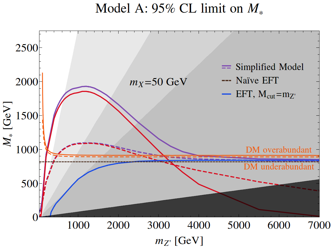
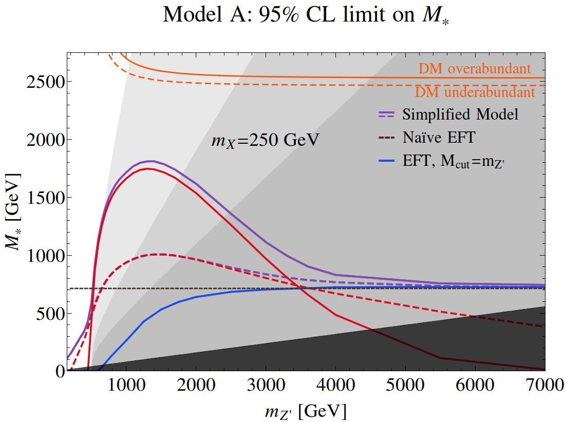
First, we can visually check that our consistent EFT limits are actually correct model-independent constraints, as they lie systematically below those obtained by working directly with the simplified model. Notice that this is not true for the naïve EFT limits, which overestimate the exclusion for very low mediator mass. Second, we observe that the limits obtained directly in Model A are slightly stronger that the EFT ones, and that this effect is considerably amplified for a moderately light mediator in the case of the smaller ratio. The reason for this behaviour is that the simplified model cross-section can get significantly enhanced with respect to the EFT one, leading to a stronger bound, only thanks to the resonant production of the mediator, which can only take place if the latter is light enough. Furthermore, the resonant enhancement is of order , and this is why it is more pronounced for a narrow mediator. These considerations are made quantitative by the solid and dashed red lines in fig. 5, with the same conventions as before. These lines represent the limits on the simplified model obtained by computing the signal rate restricting the invariant mass of the propagators within two widths from its pole mass. The fact that the red lines are so close to the purple lines representing the “true” limit, when they are both significantly above the blue line, confirms that the resonant production is what drives the enhancement. It also suggests that in this kinematical region DM searches in the simplified model should be actually regarded as mediator searches, and the results reported as limits on BR(). Also, resonant production followed by the decay into quark-antiquark pairs, leading to a peak in the di-jet invariant mass distribution, may be a complementary signal to be looked for [66, 67, 68, 69], with or without the extra jet: in such a case, we would obtain a limit on BR(). We will comment further on this in the conclusions.
We now turn to the aforementioned limitation of the plane, which was already noticed in refs. [28, 43, 52], but we find important to emphasise. Model A has four parameters: , , , . In fig. 5, the DM mass is set to a fixed value and each point of the plane uniquely determines and . Then also the product is fixed by the left-hand side of eq. (16), namely
| (18) |
Only one combination of the two couplings is left free at this point, and it might seem a good idea to fix it point-by-point to fit the values of that were assumed in drawing the purple lines in the figure. However, we must take into account that, for fixed , the accessible values of are bounded from below:
| (19) |
where and are suitably defined coefficients (see appendix A) that do not depend on and , and have only a mild dependence on the spectrum through phase space. This means that the plane is divided into regions, whose boundaries are curves (or, approximately, straight lines), where is always larger than a certain value. Some representative regions are displayed as grey shaded areas in fig. 5: from the top left to the bottom right, they correspond to . The fourth and darkest region at the bottom right corresponds to , where neither the EFT nor the simplified model admit a consistent perturbative description. In the neighbouring region where , the EFT can still be consistently used, but the same does not apply to the chosen underlying simplified model: the fact that is telling us that in such strong coupling regime the simple mediator interpretation of the origin of the effective interaction breaks down. Even in the perturbative regime, the direct simplified model lines are obtained by assuming a given , thus they become inconsistent on the right of the boundary of the corresponding region, because they cannot be associated to any physical point of the simplified model parameter space. On the left plot, for instance, we should have stopped drawing the purple and red solid lines corresponding to where they cross the boundary between the white and the very light grey region, at GeV. Similarly, we should have stopped the purple and red dashed lines, corresponding to , where they cross the boundary of the two light grey regions, at TeV. The only justification for keeping them is that the limits on the width are theoretical constraints, while the actual location of the curves is the result of the experimental analysis, which might improve its sensitivity in the future. When this will happen the exclusion curves will move up and will exit more and more out of the inconsistent regions. As far as current data are concerned, however, this observation shows that the DM limits are actually rather poor, especially in the region of narrow mediator width, which corresponds to a weakly-interacting particle. But after all, this is exactly what we concluded from our exploration of the EFT parameter space: ‘small’ effective couplings of order one are still unconstrained. Here we have just verified that the simplified model can not help us much in this respect.
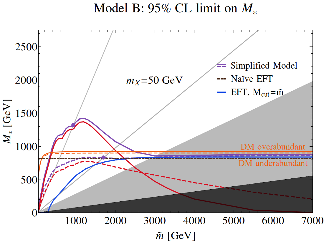
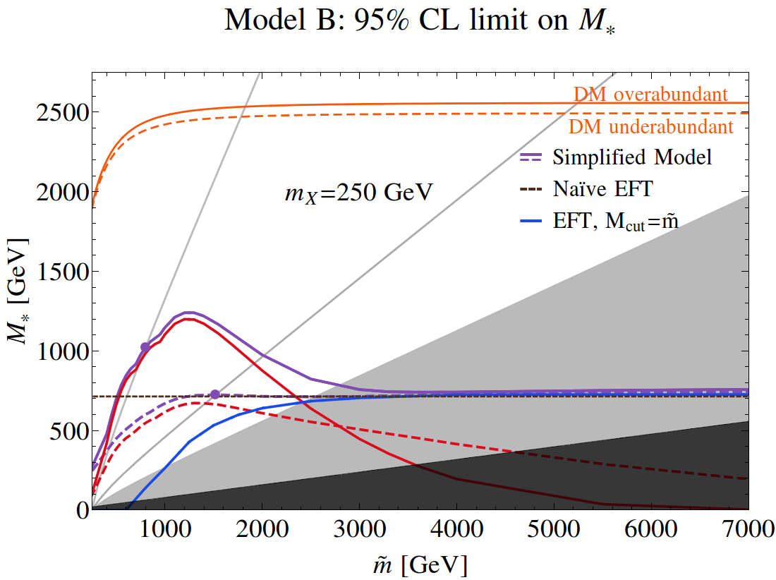
Very similar considerations apply to Model B, whose bounds are depicted in fig. 6. Also in this case the enhancement of the limit obtained directly in the simplified model is mostly due to the resonant production of the mediator, which can occur even in the so-called ‘-channel mediator’ case if an extra jet is emitted in the final state. This process corresponds (see diagrams B.3 and B.5 in fig. 4) to an associated DM- production followed by the decay into DM plus jet. Once again, in the region of Model B where the squarks are light enough, experiments should extend their selection criteria and look more generally for jets plus , to include the possibility of resonant squark production, both singly and in pairs. Of course, part of this is already being done in the context of standard squark searches within simplified supersymmetric models [70, 71]. An experimental analysis along the above lines has been recently suggested by ref. [72] within a simplified supersymmetric model with a very light gravitino: something similar could be devised also for Model B and similar simplified models for DM with ‘-channel mediators’. A second point worth stressing for Model B is that the issue with the plane is even more severe than in Model A, because the model has only three parameters, therefore after fixing , and the (width/mass) ratio of the mediator is fixed. In this case, fig. 6 shows two lines corresponding to , a grey area where where , and a dark grey area where . The only physical points of the four exclusion curves derived in Model B (purple and red, solid and dashed) are those at the intersection with the lines corresponding to the assumed value of , marked as full purple dots.
Other approaches
We are not the first to address the issues related with the naïve use of the EFT for DM in kinematical regimes extending beyond its range of validity: as already mentioned, they have been studied at length in the literature [25, 26, 27, 28, 29, 30, 31, 32, 33]. In particular, refs. [27, 29, 30] proposed a criterion (recently adopted in refs. [47, 52]) to estimate how sensitive the naïve limits on are to the unsafe region of the EFT and how much they deteriorate if the latter region is excluded from the analysis. Below we discuss two aspects of our approach in a way that can be helpful for the comparison with this previous literature.
The first point to be discussed concerns the choice of the kinematical variable to be used for discriminating the safe EFT region from the unsafe one. From the EFT viewpoint, the natural variable is clearly the hard scale of the process, : this was our choice for the present paper. However, within specific ‘mediator’ models, or more precisely classes of models, another possible choice is the variable , as proposed in refs. [27, 29, 30]. is defined as the maximal virtuality of the mediator propagator, computed over the Feynman diagrams contributing to the partonic DM production process under study. Since , using to define the safe kinematical region of the EFT means gaining signal cross-section, thus obtaining a stronger and still reliable limit. Notice that, since the definition of depends on whether the mediator propagates in the or in the channel in the two-body annihilation , is not suited for setting a model-independent limit. However, one might still consider the two possibilities in turn and set separate limits for the two cases of - and -channel mediation. While this clearly does not exhaust all possibilities 1010 10 The effective interaction might well be generated by the combined exchange of - and -channel mediators, or by radiative effects not falling in any of these two categories., it might be still worth doing if it considerably enhances the reach.
To explore the exclusion reach of this method and compare it with ours, we start by recalling the (trivial) expressions for in Models A (-channel) and B (-channel), corresponding to the diagrams in fig. 4 and the conventions in eqs. (13)–(15). In Model A, for both process I and process II (the kinematics of III is identical to that of II, so it does not need a separate discussion), is just the invariant mass of the DM pair
| (20) |
In model B, instead, we have to consider process I and II,III separately. In the case of process I, reads 1111 11 Notice that, if in Model B we had assumed a Dirac DM particle, only half of the conditions in eqs. (21) and (22) should have been imposed. Therefore, the model dependence of this strategy depends on the assumptions made both on the mediator (-channel or -channel) and on the nature of the DM particle (Dirac or Majorana fermion, complex or real scalar).
| (21) | |||||
while for process II,III we have
| (22) | |||||
Notice that the subprocesses are quantum-mechanically distinguishable and therefore it makes sense to adopt a different definition of for each of them.
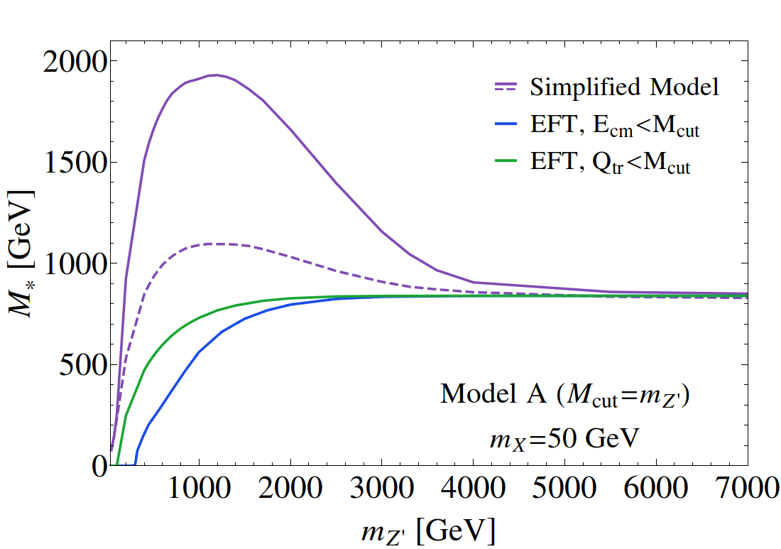
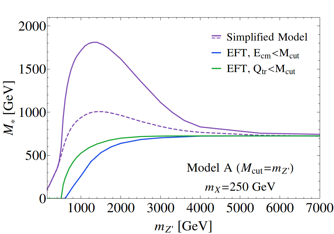
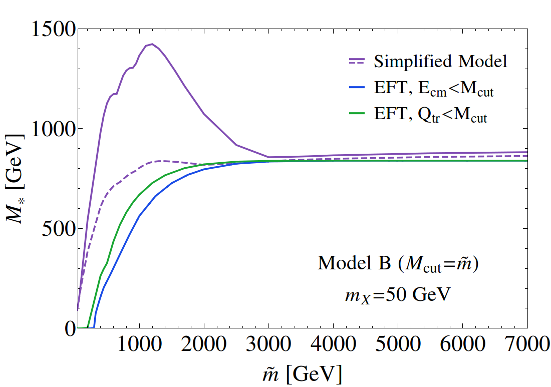
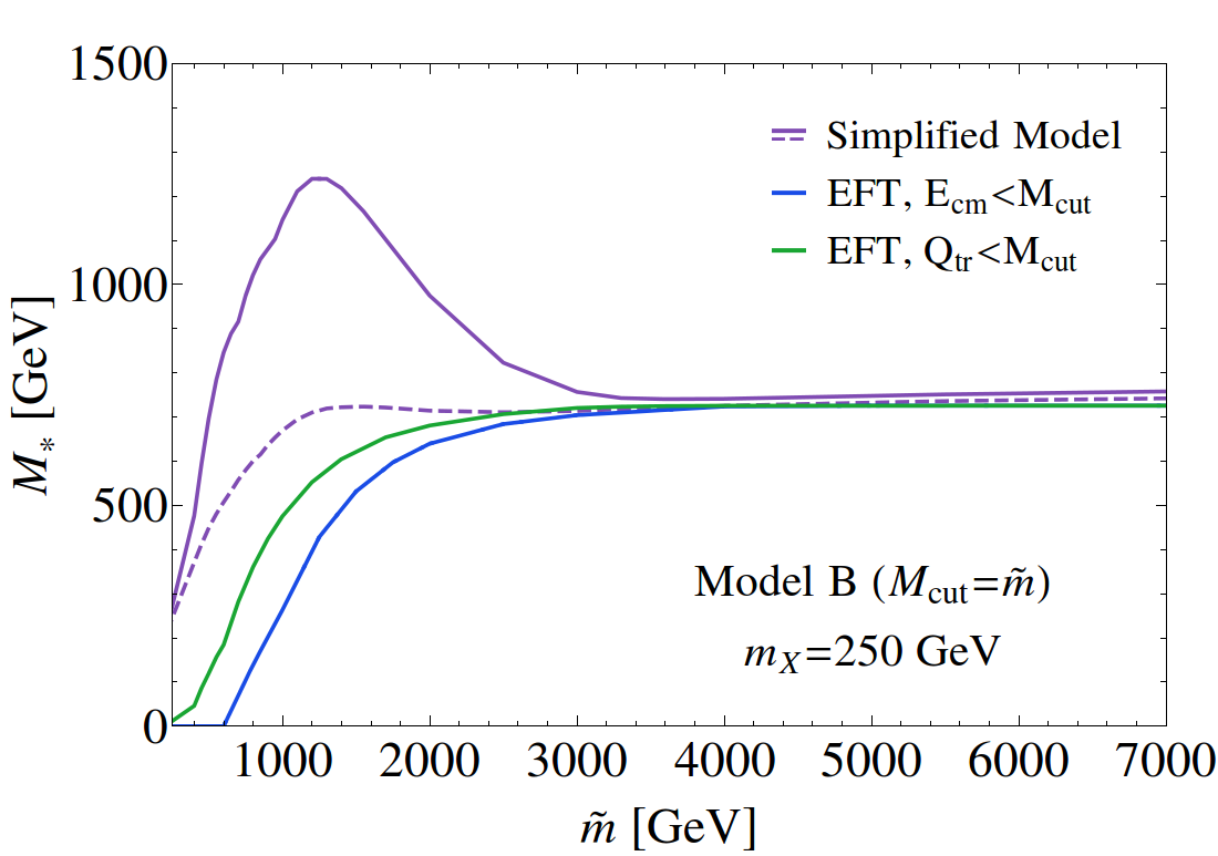
The result of the comparison is displayed in fig. 7, where we show the limits on as functions of , obtained for Models A (upper plots) and B (lower plots) with three different methods. The purple and blue lines represent the full model and our approach to the EFT, respectively, namely the same curves as in figs. 5 and 6. The green line is also derived in the EFT, but with the cut instead of . In the limit of heavy mediators, all the lines coincide as expected. The differences are in the region of relatively light mediators, where the EFT limit obtained with has, as expected, a better reach in than our method. However, in our view the improvement is not sufficiently significant, especially when compared with that obtainable in the full simplified model, to motivate the use of rather than . Our recommendation is thus to stick to the simple and model-independent version of our method, possibly trying to extend the reach by the direct search of the mediator which, as described in the previous section, is the sole responsible of the improved reach of the simplified model.
The second aspect to be clarified is that the consistent EFT limits in the plane, at fixed , cannot be inferred from those obtained in the naïve EFT by just performing a rescaling of . It is indeed clear that such a rescaling cannot lead to closed exclusion curves such as those we obtained in fig. 3. One might be tempted to consider a rescaling here because the EFT cross-section is proportional to , so that the reduction of the cross-section caused by the kinematical cut might be reabsorbed into an effective . Namely, one might consider defining the ratio 1212 12 Using or makes no difference for the point we want to make here.
| (23) |
where denotes the signal cross-section computed in the naïve EFT for a given signal region. At fixed and , is a function of , which tends to one for sufficiently high and to zero for sufficiently low , because of the effect of the kinematical cut illustrated in eq. (11). Given that measures the reduction of the cross-section with respect to the naïve EFT, one might think of getting the limit on at each , call it , starting from the limit obtained in the naïve EFT, call it , and solving the implicit equation
| (24) |
The effective operator scale obtained in this way is the one that reproduces, in the EFT with the cut on , the same signal cross-section that was needed for setting the bound at in the naïve EFT. Namely, eq. (24) is equivalent to
| (25) |
where we have exploited the fact that in the naïve EFT simply scales as .
The above method for obtaining is more elaborate than directly comparing the experimental limit on the cross-section with the prediction of the kinematically restricted EFT, as we suggested in section 2.1. Furthermore, the rescaling method might obscure the fact that eq. (25), or equivalently eq. (24), has either zero (which means that no limit can be set) or two solutions for , but it never has only one. The behaviour of the restricted EFT cross-section, compared with the naïve EFT, is pictorially represented in fig. 8.

The cross-section vanishes before approaching , because of the cut . Therefore there are two values of for which the cross-section equals the experimental limit, which means that the excluded region has one upper but also one lower limit in , differently from the naïve EFT as depicted in the figure. Therefore, the true limit cannot be set by just rescaling the naïve EFT exclusion curve. Notice also that certain strategies to solve eq. (24), such as applying an iterative procedure starting from , might obscure the existence of the lower bound, as they systematically converge to the upper one. The quantitative impact on the excluded regions in the plane, for different values of , was already displayed in fig. 3 for our kinematical requirement .
4 Conclusions
We described a simple strategy to set robust and model-independent limits on heavy-mediator DM at the LHC. Our method is based on the generic form of the operators in the EFT containing only the DM and the SM particles, with no assumptions on the underlying dynamics. However, it also takes into account the presence of a cutoff scale above which the EFT loses its validity. must be regarded as one of the free parameters of the EFT, on the same footing as the DM mass and the effective interaction scale . We have to do so if we aim at a comprehensive exploration of the whole range of theoretical possibilities. The parameter can be traded for , the typical coupling strength at the mediator scale. As explained in the paper, can be defined in the EFT alone, and further characterised for any assumed underlying model.
We applied our method explicitly to the ATLAS mono-jet search of ref. [42], obtaining the exclusion contours in the plane shown in fig. 3, for fixed representative values of . We believe that this kind of plots illustrates the current experimental situation in an accurate and comprehensive way, providing a fair assessment of the LHC sensitivity to heavy-mediator DM. At the moment, we are only sensitive to large values of , while the region , which is arguably the most natural one for WIMP DM, is still largely untested. Making progress requires higher energy and luminosity, but also an optimisation of the experimental search strategies. As pointed out in section 2, our signal is kinematically different from that of the naïve EFT, in particular it is characterised by softer and distributions. The reach of the searches would then benefit from a sensitivity improvement in the soft region.
In section 3 we considered two different simplified models, both giving rise to the same effective operator considered in section 2. We compared our EFT limits, reinterpreted in the two models, with those obtained from a dedicated comparison of the experimental bounds with the prediction of the two models, reaching two main conclusions. First, the limits set within the simplified models can be considerably stronger than the EFT ones, but only because of the resonant production of the mediator, which enhances the simplified model cross-section. Therefore, a DM search performed within a simplified model (in the only interesting region where the limit is potentially stronger than in the EFT) is actually not a search for DM, but a search for the mediator, and as such it should be interpreted. The canonical BR limit as a function of the mediator mass appears to be the best option for presenting the experimental results. The second conclusion is that the current experimental sensitivity is still rather poor, even when working within a simplified model. In particular the region of weak coupling, i.e. narrow mediator, is mostly unexplored, in accordance with what we found in our EFT analysis. We finally discussed two aspects of our approach, to facilitate the comparison with the recent literature. We found that the usage of the variable in place of to define the safe kinematical region of the EFT does not improve the sensitivity significantly enough to pay back for the increased model-dependence. We also remarked that just rescaling the naïve EFT limit does not account for the impossibility, within mono-jet searches, of excluding arbitrarily low values of at fixed and .
In summary, we have found that the LHC sensitivity to the heavy-mediator DM hypothesis is still limited and wide regions of the parameter space still wait to be explored. On the experimental side, improving the analysis in the soft region would be of great help. On the phenomenological side, more comprehensive methods should be elaborated to cover each different region of the parameter space with the most suitable strategy. Non-resonant DM signals are well described by the EFT which, as outlined in the present paper, when consistently used provides a robust model-independent way to approach the problem. Within specific models, this needs to be supplemented by resonant mediator searches, which however should be performed by exploiting fully the predictive power of the assumed mediator dynamics. This means taking into account all the mediator production mechanisms (single and/or pair) and all its possible decay modes, including the one to visible objects which might give complementary informations. These aspects are left to future work.
Acknowledgements.
We thank A. De Simone, M. de Vries, E. Morgante, T. Jacques, G. Polesello, S. Rahatlou, A.W. Riotto, F. Riva, A. Romanino, A. Urbano, and M. Zanetti for discussions. We acknowledge Heidi for computational support. This work was supported in part by the ERC Advanced Grant no.267985 (DaMeSyFla), by the MIUR-PRIN project 2010YJ2NYW and by the MIUR-FIRB Grant RBFR12H1MW.Appendix A Model A: axial-vector mediator
We collect here some details on the first of the two simplified models considered in the text, Model A. Previous discussions of very similar models can be found in refs. [54, 55, 56, 57, 58, 59]. The mediator is a neutral vector boson , singlet under the SM gauge group, with mass , a universal axial coupling to quarks, no renormalisable couplings to leptons, and an axial coupling to the Majorana DM fermion of mass . Since the model is introduced for purely illustrative purposes, without making reference to an underlying more fundamental theory, we introduce an explicit mass term and we neglect - mixing, as well as anomalies and their cancellation mechanisms.
The model Lagrangian is
| (26) | |||||
| (27) | |||||
| (28) |
where is the SM Lagrangian, is the free Lagrangian for in (5), , and the sum in (28) runs over all quark flavours (). The model has four parameters,
| (29) |
which can all be taken to be real and positive (in principle, and could have either sign, but this is not relevant for the present study).
Notice that the choice of a purely axial interaction, universal for all quark flavours, is crucial to generate the effective interaction (6) from (28) in the low-energy limit. At leading order in , the approximate solution of the equations of motion is
which substituted in (26) gives
| (30) | |||||
| (31) | |||||
| (32) |
The effective interaction term (32) between the SM quarks and the DM field reproduces the one in (6) as long as
| (33) |
Notice also that integrating out the heavy generates two additional four-fermion operators, (30) and (31). However, (30) is subject only to very mild constraints from the limits on DM self-interactions. The four-quark operator (31) can be probed by the searches for contact interactions [73, 74], but can be parametrically suppressed by choosing for fixed .
At tree-level, and including only two-body decays, the total decay width of the is
| (34) |
with the obvious modifications if some of the final states are not kinematically accessible.
Appendix B Model B: coloured scalar mediators
We collect here some details on the second of the two simplified models considered in the text, Model B. Previous discussions of very similar models can be found in refs. [60, 61, 62, 63, 64, 65]. In Model B, the interactions between the SM quarks and the DM particle X are mediated by three families of degenerate complex scalars of mass , with the same gauge quantum numbers of the corresponding left- and right-handed quarks. Since they are identical to the squarks of supersymmetric extensions of the SM, we denote them with the same symbols, (), where are family indices. Similarly, the Majorana fermion mimicks, although in the simplified fashion specified by its interactions below, the lightest neutralino of supersymmetric models.
The model Lagrangian reads
| (35) | |||||
| (36) | |||||
| (37) |
where and are the same as in Model A, and the dots in (36) denote the squark gauge interactions, generated by promoting ordinary derivatives to SM covariant derivatives. Notice that the mass degeneracy and the universality of the Yukawa couplings among quarks, squarks and DM evade the typical problems of supersymmetric models with flavour-changing neutral currents. The model has three parameters,
| (38) |
which can all be taken to be real and positive ( can be complex, but it can be chosen to be real and positive by absorbing its phase into a redefinition of the squark fields).
As for Model A, we can derive the EFT by solving the classical equations of motion for the squarks in the low-energy limit :
| (39) |
Substituting into yields
| (40) | |||||
where for the second equality we have used the Fierz identities and the fact that when is a Majorana spinor . The effective interaction term (40) between the SM quarks and the DM particle reproduces the one in (6) as long as
| (41) |
At tree-level, and assuming , where is the corresponding quark, the decay width of the generic is
| (42) |
Appendix C Formulae for the relic density
We collect here the approximate analytical formulae used for the calculation of the relic density in the EFT (fig. 2), in Model A (fig. 5) and in Model B (fig. 6), before requiring that it reproduces the recent precise determination by the Planck collaboration [75] (for our purposes, the latter can be rounded to with negligible error). They can be straightforwardly derived from the existing literature (see e.g. [76, 77]). Up to terms of order , where is the value of at freeze-out:
| (43) |
where is the dimensionless Hubble parameter, is the number of relativistic degrees of freedom, is the reduced Planck mass, is the mass of the DM particle in GeV, and
| (44) | |||||
| (45) |
In the EFT, introducing the dimensionless parameters ,
| (46) | |||||
| (47) |
where the sums run over the quark flavours whose mass is below .
In the two models underlying the EFT, we introduce two additional dimensionless parameters, and , to account for the finite mass and width of the mediator. Then in Model A ( mediator)
| (48) | |||||
| (49) | |||||
and in Model B ( mediator)
| (50) | |||||
| (51) | |||||
References
- (1) G. Aad et al. [ATLAS Collaboration], Observation of a new particle in the search for the Standard Model Higgs boson with the ATLAS detector at the LHC, Phys. Lett. B 716 (2012) 1 [arXiv:1207.7214 [hep-ex]].
- (2) S. Chatrchyan et al. [CMS Collaboration], Observation of a new boson at a mass of 125 GeV with the CMS experiment at the LHC, Phys. Lett. B 716 (2012) 30 [arXiv:1207.7235 [hep-ex]].
- (3) M. Kado (ATLAS Collaboration), Physics of the Brout-Englert-Higgs boson in ATLAS, plenary talk at ICHEP 2014, Valencia, Spain, 2-9 July 2014, to appear in the Proceedings.
- (4) A. David (CMS Collaboration), Physics of the Brout-Englert-Higgs boson in CMS, plenary talk at ICHEP 2014, Valencia, Spain, 2-9 July 2014, to appear in the Proceedings.
- (5) F. Würthwein, Results on Physics Beyond the Standard Model from ATLAS and CMS, plenary talk at ICHEP 2014, Valencia, Spain, 2-9 July 2014, to appear in the Proceedings.
- (6) D. Whiteson, Dark Matter Collider Searches, Lectures given at the 42nd SLAC Summer Institute, Stanford, USA, 4-15 August 2014.
- (7) M. W. Goodman and E. Witten, Detectability of Certain Dark Matter Candidates, Phys. Rev. D 31 (1985) 3059.
- (8) A. Birkedal, K. Matchev and M. Perelstein, Dark matter at colliders: A Model independent approach, Phys. Rev. D 70 (2004) 077701 [hep-ph/0403004].
- (9) M. Beltran, D. Hooper, E. W. Kolb and Z. C. Krusberg, Deducing the nature of dark matter from direct and indirect detection experiments in the absence of collider signatures of new physics, Phys. Rev. D 80 (2009) 043509 [arXiv:0808.3384 [hep-ph]].
- (10) Q. H. Cao, C. R. Chen, C. S. Li and H. Zhang, Effective Dark Matter Model: Relic density, CDMS II, Fermi LAT and LHC, JHEP 1108 (2011) 018 [arXiv:0912.4511 [hep-ph]].
- (11) M. Beltran, D. Hooper, E. W. Kolb, Z. A. C. Krusberg and T. M. P. Tait, Maverick dark matter at colliders, JHEP 1009 (2010) 037 [arXiv:1002.4137 [hep-ph]];
- (12) J. Goodman, M. Ibe, A. Rajaraman, W. Shepherd, T. M. P. Tait and H. B. Yu, Constraints on Light Majorana dark Matter from Colliders, Phys. Lett. B 695 (2011) 185 [arXiv:1005.1286 [hep-ph]].
- (13) Y. Bai, P. J. Fox and R. Harnik, The Tevatron at the Frontier of Dark Matter Direct Detection, JHEP 1012 (2010) 048 [arXiv:1005.3797 [hep-ph]];
- (14) A. Rajaraman, W. Shepherd, T. M. P. Tait and A. M. Wijangco, LHC Bounds on Interactions of Dark Matter, Phys. Rev. D 84 (2011) 095013 [arXiv:1108.1196 [hep-ph]].
- (15) J. Goodman, M. Ibe, A. Rajaraman, W. Shepherd, T. M. P. Tait and H. B. Yu, Constraints on Dark Matter from Colliders, Phys. Rev. D 82 (2010) 116010 [arXiv:1008.1783 [hep-ph]].
- (16) P. J. Fox, R. Harnik, J. Kopp and Y. Tsai, Missing Energy Signatures of Dark Matter at the LHC, Phys. Rev. D 85 (2012) 056011 [arXiv:1109.4398 [hep-ph]].
- (17) A. Crivellin, F. D’Eramo and M. Procura, New Constraints on Dark Matter Effective Theories from Standard Model Loops, Phys. Rev. Lett. 112 (2014) 191304 [arXiv:1402.1173 [hep-ph]].
- (18) S. Davidson, Including the Z in an Effective Field Theory for dark matter at the LHC, JHEP 1410 (2014) 84 [arXiv:1403.5161 [hep-ph]].
- (19) F. D’Eramo and M. Procura, Connecting Dark Matter UV Complete Models to Direct Detection Rates via Effective Field Theory, arXiv:1411.3342 [hep-ph].
- (20) M. Duch, B. Grzadkowski and J. Wudka, Classification of effective operators for interactions between the Standard Model and dark matter, arXiv:1412.0520 [hep-ph].
- (21) J. Fan, M. Reece and L. T. Wang, Non-relativistic effective theory of dark matter direct detection, JCAP 1011 (2010) 042 [arXiv:1008.1591 [hep-ph]].
- (22) A. L. Fitzpatrick, W. Haxton, E. Katz, N. Lubbers and Y. Xu, The Effective Field Theory of Dark Matter Direct Detection, JCAP 1302 (2013) 004 [arXiv:1203.3542 [hep-ph]].
- (23) A. L. Fitzpatrick, W. Haxton, E. Katz, N. Lubbers and Y. Xu, Model Independent Direct Detection Analyses, arXiv:1211.2818 [hep-ph].
- (24) M. Cirelli, E. Del Nobile and P. Panci, Tools for model-independent bounds in direct dark matter searches, JCAP 1310 (2013) 019 [arXiv:1307.5955 [hep-ph]].
- (25) P. J. Fox, R. Harnik, J. Kopp and Y. Tsai, Missing Energy Signatures of Dark Matter at the LHC, Phys. Rev. D 85 (2012) 056011 [arXiv:1109.4398 [hep-ph]].
- (26) A. Friedland, M. L. Graesser, I. M. Shoemaker and L. Vecchi, Probing Nonstandard Standard Model Backgrounds with LHC Monojets, Phys. Lett. B 714 (2012) 267 [arXiv:1111.5331 [hep-ph]].
- (27) G. Busoni, A. De Simone, E. Morgante and A. Riotto, On the Validity of the Effective Field Theory for Dark Matter Searches at the LHC, Phys. Lett. B 728 (2014) 412 [arXiv:1307.2253 [hep-ph]].
- (28) O. Buchmueller, M. J. Dolan and C. McCabe, Beyond Effective Field Theory for Dark Matter Searches at the LHC, JHEP 1401 (2014) 025 [arXiv:1308.6799 [hep-ph]].
- (29) G. Busoni, A. De Simone, J. Gramling, E. Morgante and A. Riotto, On the Validity of the Effective Field Theory for Dark Matter Searches at the LHC, Part II: Complete Analysis for the -channel, JCAP 1406 (2014) 060 [arXiv:1402.1275 [hep-ph]].
- (30) G. Busoni, A. De Simone, T. Jacques, E. Morgante and A. Riotto, On the Validity of the Effective Field Theory for Dark Matter Searches at the LHC Part III: Analysis for the -channel, JCAP09(2014)022 [arXiv:1405.3101 [hep-ph]].
- (31) C. Englert and M. Spannowsky, Effective Theories and Measurements at Colliders, Phys. Lett. B 740 (2015) 8 [arXiv:1408.5147 [hep-ph]].
- (32) J. Abdallah, A. Ashkenazi, A. Boveia, G. Busoni, A. De Simone, C. Doglioni, A. Efrati and E. Etzion et al., Simplified Models for Dark Matter and Missing Energy Searches at the LHC, arXiv:1409.2893 [hep-ph].
- (33) S. Malik, C. McCabe, H. Araujo, A. Belyaev, C. Boehm, J. Brooke, O. Buchmueller and G. Davies et al., Interplay and Characterization of Dark Matter Searches at Colliders and in Direct Detection Experiments, arXiv:1409.4075 [hep-ex].
- (34) M. R. Buckley, D. Feld and D. Goncalves, Scalar Simplified Models for Dark Matter, Phys. Rev. D 91 (2015) 1, 015017 [arXiv:1410.6497 [hep-ph]].
- (35) A. Biekoetter, A. Knochel, M. Kraemer, D. Liu and F. Riva, Vices and Virtues of Higgs EFTs at Large Energy, arXiv:1406.7320 [hep-ph].
- (36) U. Haisch and F. Kahlhoefer, On the importance of loop-induced spin-independent interactions for dark matter direct detection, JCAP 1304 (2013) 050 [arXiv:1302.4454 [hep-ph]].
- (37) A. Crivellin, F. D’Eramo and M. Procura, New Constraints on Dark Matter Effective Theories from Standard Model Loops, Phys. Rev. Lett. 112 (2014) 191304 [arXiv:1402.1173 [hep-ph]].
- (38) S. Chatrchyan et al. [CMS Collaboration], Search for New Physics with a Mono-Jet and Missing Transverse Energy in Collisions at TeV, Phys. Rev. Lett. 107 (2011) 201804 [arXiv:1106.4775 [hep-ex]].
- (39) G. Aad et al. [ATLAS Collaboration], Search for new phenomena with the monojet and missing transverse momentum signature using the ATLAS detector in TeV proton-proton collisions, Phys. Lett. B 705 (2011) 294 [arXiv:1106.5327 [hep-ex]].
- (40) S. Chatrchyan et al. [CMS Collaboration], Search for dark matter and large extra dimensions in monojet events in collisions at TeV, JHEP 1209 (2012) 094 [arXiv:1206.5663 [hep-ex]].
- (41) G. Aad et al. [ATLAS Collaboration], Search for dark matter candidates and large extra dimensions in events with a jet and missing transverse momentum with the ATLAS detector, JHEP 1304 (2013) 075 [arXiv:1210.4491 [hep-ex]].
- (42) G. Aad et al. [ATLAS Collaboration], Search for New Phenomena in Monojet plus Missing Transverse Momentum Final States using 10fb-1 of pp Collisions at TeV with the ATLAS detector at the LHC, ATLAS-CONF-2012-147.
- (43) V. Khachatryan et al. [CMS Collaboration], Search for dark matter, extra dimensions, and unparticles in monojet events in proton-proton collisions at = 8 TeV, arXiv:1408.3583 [hep-ex].
- (44) S. Chatrchyan et al. [CMS Collaboration], Search for Dark Matter and Large Extra Dimensions in pp Collisions Yielding a Photon and Missing Transverse Energy, Phys. Rev. Lett. 108 (2012) 261803 [arXiv:1204.0821 [hep-ex]].
- (45) G. Aad et al. [ATLAS Collaboration], Search for dark matter candidates and large extra dimensions in events with a photon and missing transverse momentum in collision data at TeV with the ATLAS detector, Phys. Rev. Lett. 110 (2013) 1, 011802 [arXiv:1209.4625 [hep-ex]].
- (46) V. Khachatryan et al. [CMS Collaboration], Search for new phenomena in monophoton final states in proton-proton collisions at = 8 TeV, arXiv:1410.8812 [hep-ex].
- (47) G. Aad et al. [ATLAS Collaboration], Search for new phenomena in events with a photon and missing transverse momentum in collisions at TeV with the ATLAS detector, arXiv:1411.1559 [hep-ex].
- (48) G. Aad et al. [ATLAS Collaboration], Search for dark matter in events with a hadronically decaying W or Z boson and missing transverse momentum in collisions at 8 TeV with the ATLAS detector, Phys. Rev. Lett. 112 (2014) 4, 041802 [arXiv:1309.4017 [hep-ex]].
- (49) G. Aad et al. [ATLAS Collaboration], Search for dark matter in events with a Z boson and missing transverse momentum in pp collisions at =8 TeV with the ATLAS detector, Phys. Rev. D 90 (2014) 1, 012004 [arXiv:1404.0051 [hep-ex]].
- (50) G. Aad et al. [ATLAS Collaboration], Search for dark matter in events with heavy quarks and missing transverse momentum in collisions with the ATLAS detector, arXiv:1410.4031 [hep-ex].
- (51) G. Aad et al. [ATLAS Collaboration], Search for invisible particles produced in association with single-top-quarks in proton-proton collisions at = 8 TeV with the ATLAS detector, arXiv:1410.5404 [hep-ex].
- (52) G. Aad et al. [ATLAS Collaboration], Search for new phenomena in final states with an energetic jet and large missing transverse momentum in pp collisions at TeV with the ATLAS detector, arXiv:1502.01518 [hep-ex].
- (53) J. Alwall, R. Frederix, S. Frixione, V. Hirschi, F. Maltoni, O. Mattelaer, H.-S. Shao and T. Stelzer et al., The automated computation of tree-level and next-to-leading order differential cross sections, and their matching to parton shower simulations, JHEP 1407 (2014) 079 [arXiv:1405.0301 [hep-ph]].
- (54) M. L. Graesser, I. M. Shoemaker and L. Vecchi, A Dark Force for Baryons, arXiv:1107.2666 [hep-ph].
- (55) H. An, X. Ji and L. T. Wang, Light Dark Matter and Dark Force at Colliders, JHEP 1207 (2012) 182 [arXiv:1202.2894 [hep-ph]].
- (56) A. Alves, S. Profumo and F. S. Queiroz, The dark portal: direct, indirect and collider searches, JHEP 1404 (2014) 063 [arXiv:1312.5281 [hep-ph]].
- (57) O. Lebedev and Y. Mambrini, Axial Dark Matter: the case for an invisible , arXiv:1403.4837 [hep-ph].
- (58) D. Hooper, Z’ Mediated Dark Matter Models for the Galactic Center Gamma-Ray Excess, arXiv:1411.4079 [hep-ph].
- (59) J. Blumenthal, P. Gretskov, M. Krämer and C. Wiebusch, Effective field theory interpretation of searches for dark matter annihilation in the Sun with the IceCube Neutrino Observatory, arXiv:1411.5917 [astro-ph.HE].
- (60) S. Chang, R. Edezhath, J. Hutchinson and M. Luty, Effective WIMPs, Phys. Rev. D 89 (2014) 015011 [arXiv:1307.8120 [hep-ph]].
- (61) H. An, L. T. Wang and H. Zhang, Dark matter with -channel mediator: a simple step beyond contact interaction, Phys. Rev. D 89 (2014) 115014 [arXiv:1308.0592 [hep-ph]].
- (62) A. DiFranzo, K. I. Nagao, A. Rajaraman and T. M. P. Tait, Simplified Models for Dark Matter Interacting with Quarks, JHEP 1311 (2013) 014 [arXiv:1308.2679 [hep-ph]].
- (63) M. Papucci, A. Vichi and K. M. Zurek, Monojet versus rest of the world I: t-channel Models, arXiv:1402.2285 [hep-ph].
- (64) M. Garny, A. Ibarra, S. Rydbeck and S. Vogl, Majorana Dark Matter with a Coloured Mediator: Collider vs Direct and Indirect Searches, JHEP 1406 (2014) 169 [arXiv:1403.4634 [hep-ph]].
- (65) P. Harris, V. V. Khoze, M. Spannowsky and C. Williams, Constraining Dark Sectors at Colliders: Beyond the Effective Theory Approach, [arXiv:1411.0535 [hep-ph]].
- (66) B. A. Dobrescu and F. Yu, Coupling-mass mapping of dijet peak searches, Phys. Rev. D 88 (2013) 3, 035021 [arXiv:1306.2629 [hep-ph]].
- (67) S. Chatrchyan et al. [CMS Collaboration], Search for narrow resonances using the dijet mass spectrum in pp collisions at =8 TeV, Phys. Rev. D 87, no. 11, 114015 (2013) [arXiv:1302.4794 [hep-ex]].
- (68) G. Aad et al. [ATLAS Collaboration], Search for new phenomena in the dijet mass distribution using collision data at TeV with the ATLAS detector, arXiv:1407.1376 [hep-ex].
- (69) V. Khachatryan et al. [CMS Collaboration], Search for resonances and quantum black holes using dijet mass spectra in proton-proton collisions at =8 TeV, arXiv:1501.04198 [hep-ex].
- (70) S. Chatrchyan et al. [CMS Collaboration], Search for new physics in the multijet and missing transverse momentum final state in proton-proton collisions at = 8 TeV, JHEP 1406, 055 (2014) [arXiv:1402.4770 [hep-ex]].
- (71) G. Aad et al. [ATLAS Collaboration], Search for squarks and gluinos with the ATLAS detector in final states with jets and missing transverse momentum using TeV proton–proton collision data, JHEP 1409, 176 (2014) [arXiv:1405.7875 [hep-ex]].
- (72) F. Maltoni, A. Martini, K. Mawatari and B. Oexl, Signals of a superlight gravitino at the LHC, arXiv:1502.01637 [hep-ph].
- (73) H. Dreiner, D. Schmeier and J. Tattersall, Contact Interactions Probe Effective Dark Matter Models at the LHC, Europhys. Lett. 102 (2013) 51001 [arXiv:1303.3348 [hep-ph]].
- (74) M. de Vries, Four-Quark Effective Operators at Hadron Colliders, arXiv:1409.4657 [hep-ph].
- (75) P. A. R. Ade et al. [Planck Collaboration], Planck 2013 results. XVI. Cosmological parameters, Astron. Astrophys. 571 (2014) A16 [arXiv:1303.5076 [astro-ph.CO]].
- (76) E. W. Kolb and M. S. Turner, The early universe, Redwood City, Addison-Wesley (1990).
- (77) P. Gondolo and G. Gelmini, Cosmic abundances of stable particles: improved analysis, Nucl. Phys. B360 (1991) 145-179.