Localization principle in SUSY gauge theories
Abstract
Localization principle is a powerful analytic tool in supersymmetric gauge theories which enables one to perform supersymmetric path integrals explicitly. Many important formulae have been obtained, and they led to a major breakthrough in the understanding of gauge theories at strong coupling as well as the dynamics of branes in M-theory. Some of those results are reviewed, focusing especially on Pestun’s solution to four-dimensional supersymmetric gauge theories on and the subsequent developments on three or four-dimensional gauge theories on spheres.
PTEP-subject
xxxx, xxx1 Introduction
Localization is a powerful mathematical principle that sometimes allows us to reduce the difficulty of integrals over complicated spaces. If a continuous symmetry acts on the space, one can express certain integrals over that space as sums of contributions from fixed points, that is the points which are invariant under the symmetry. It has been applied to the problems in supersymmetric gauge theories in different ways, and led to a number of useful formulae that can plobe the strong coupling dynamics of gauge theories.
What is localization principle
Let us explain the basic idea of localization principle, quoting an illustrative example of the volume of sphere from [1]. We use the standard polar coordinates on the sphere , in terms of which the simplectic volume form is given by . Using the rotational symmetry generated by the vector field , one can think of a deformation of the ordinary derivative into an equivariant derivative , and accordingly deform the ordinary closed forms into the differential forms annihilated by , called equivariantly closed forms. The volume form is then modified into , where is the Hamiltonian function for the isometry . The symplectic volume of then receives the following modification,
| (1) |
Interestingly, in the rightmost expression the two terms can be interpreted as contributions from two fixed points, namely the north and the south poles. Indeed, one can “approximate” the contribution from the north pole by a Gaussian integral over local Cartesian coordinate ,
| (2) |
where is the classical value of at the north pole and is the result of Gaussian integration over . The same approximation at the south pole and suitable Wick rotation of the integration contour can explain the other term. This example is the simplest application of localization principle or Duistermaat-Heckman’s formula in mathematics.
In string theory or quantum field theories, complicated spaces often arise as moduli space of solutions to some field equations such as BPS conditions in supersymemtric models. The integrals over such moduli spaces often provide a useful low-energy approximation to the original path integral. Actually, in some supersymmetric theories one can deform the theory in a suitable manner so that the moduli space approximation becomes exact. An example of such deformations is the topological twist of four-dimensional supersymmetric gauge theories, which was invented for studying the cohomology of instanton moduli spaces within the framework of quantum field theory [2]. Another example is the topological A-twist of 2D supersymmetric sigma models and the corresponding topological string, which involve integrals over moduli space of holomorphic maps from Riemann surfaces to Calabi-Yau manifolds [3].
In the above examples, the reduction from infinite-dimensional path integrals to finite dimensional integrals makes use of the idea of localization based on a fermionic symmetry (supersymmetry) . The supersymmetry means the action functional is invariant under , and also the path integral measure is such that the expectation values of -exact observables all vanish.
| (3) |
These imply that the values of supersymmetric observables do not change under deformations of the theory of the form for arbitrary parameter and fermionic functional such that . The supersymmetric path integrals thus localize to saddle points characterized by the BPS-like condition
| (4) |
To evaluate the contribition from each saddle point, one only needs to path integrate over fluctuations with Gaussian approximation, keeping only terms in up to the second order in the fluctuations as was done in (2). This gives an exact answer because the supersymmetric observables are -independent.
Thus in supersymmetric theories, localization is applied for two different purposes. One is the reduction from infinite-dimensional path integral to a finite dimensional integral over moduli spaces (called SUSY localization in this article), and the other is the simplification of integrals over complicated moduli spaces using symmetry (equivariant localization). The underlying principle is the same: in particular they are both characterized by a fermionic operator which squares to a bosonic symmetry of the system.
Localization in SUSY gauge theories
The two kinds of localization both played important role in [4] where Nekrasov proposed the topologically twisted gauge theory on Omega background . In this theory, the supercharge squares into a spacetime rotation plus a constant gauge rotation,
| (5) |
where is the expectation value of the scalar field in vector multiplet which parametrizes the Coulomb branch moduli space. The path integral of this theory defines the so-called Nekrasov’s instanton partition function, which is the generating function for equivariant integrals over instanton moduli spaces. The parameters play the same role as that of in (1), and simplifies the integrals over instanton moduli spaces to combinatoric sums. Nekrasov’s partition function is known to contain the information on the low energy effective prepotential; in fact there is an extensive study showing it encodes even richer information on the mathematical structure underlying 4D supersymmetric gauge theories. See [5] for a review on this field.
In 2007, the idea of SUSY localization was first applied to gauge theories which are not topological field theories. In [6] Pestun used the localization principle to obtain an exact formula for supersymmetric observables in 4D SUSY gauge theories on the sphere . He showed that the infinite dimensional path integral can be reduced to a finite-dimensional integral over Lie algebra, and using the result he gave an analytic proof of the long standing conjecture about the Wilson loops in super Yang-Mills theories [7, 8]. In 2009, another exact formulae was found for 3D superconformal Chern-Simons matter theories by Kapustin, Willett and Yaakov [9]. Together with the application of localization to the 3D superconformal index by Seok Kim [10], these work brought the power of localization to the attention of many physicists.
This article is a brief review of the pioneering work [6] and [9] and the subsequent developments in supersymmetric gauge theories based on localization principle. In the first part we will focus mostly on theories in 4 and 3 dimensions and the developments around exact partition functions on sphere. In the latter part we will discuss interesting developments regarding supersymmetric deformation of the round sphere called squasings.
Remark
SUSY localization reduces the path integral to an integral over the space of saddle points, and allows us to treat the fluctuations around saddle points by Gaussian approximation. The Gaussian integral in field theory gives rise to determinants of Laplace or Dirac operators, which are usually defined as infinite products over eigenvalues. In the following we will see many formulae for the determinants. On the face of it those infinite product formulae do not make sense or they are simply diverging, but they do make sense by a suitable regularization. Let us not worry too much about the regularization issue, instead recall that the same kind of infinite product arises even for the path-integral evaluation of partition function for a single harmonic oscillator.
| (6) |
The infinite product is understood as the result of path integration over Fourier modes of the periodic variable . It needs an appropriate regularization so as to reproduce the desired result .
2 4D gauge theories
For 4D supersymmetric gauge theories, exact partition function was obtained for topologically twisted theories on Omega background in [4]. Based on this result, Pestun [6] obtained the closed formula for supersymmetric observables on . A little later there was a development in the construction and classification of superconformal theories based on the picture of wrapped M5-branes, which led to a new understanding of the relation between gauge theories and the geometry of Riemann surface [11]. These development also led to a discovery of a surprising relation between observables in 4D gauge theories and 2D conformal field theories [12, 13].
Exact solution on
Let us begin by reviewing the exact results for the theories on . In [6], the theories was constructed by using the conformal map from flat . The supersymemtry is characterized by conformal Killing spinors satisfying
| (7) |
The indices (usually suppressed) represent they are spinors under four-dimensional rotation group, whereas the index is for doublets under R-symmetry. See [14] for our convention of spinor calculus here. In theories with rigid supersymmetry on curved spaces such as spheres, these Killing spinors appear in SUSY transformation rule in place of constant spinor parameters. Unlike the supersymmetry parameters for theories on flat they are in general not constant. But they take a fixed form once the diffeomorphism and other local gauge invariance are fixed.
theory has two supermultiplets. Vector multiplet consists of a vector , a complex scalar , gauginos and auxiliary scalar fields. Hypermultiplet consists of an doublet scalar , fermions and auxiliary fields. Once the gauge group and representation for hypermultiplet are specified, one can construct supersymmetric Laglangian for vector multiplet,
| (8) |
and the kinetic Lagrangian for hypermultiplets coupled to vector multiplets. One can also include the hypermultiplet mass term (or other SUSY invariant called FI term which we will not discuss here) in the action. The partition function will then be a function of gauge coupling , the matter mass and the radius of the sphere.
The existence of SUSY theories on spheres was known and even used in the study of superconformal indices or construction of superstring worldsheet theories. But the notion of conformal Killing spinors and the fully explicit construction of supersymmetric gauge theories on the sphere looked new and rather surprising.
To apply SUSY localization, one first chooses a specific Killing spinor . For generic choice there are two special points on , the north and south poles, characterized respectively by and . If the is defined by
| (9) |
then one can put the north pole at and the south pole at using conformal symmetry. The square of the corresponding supersymmetry yields the sum of rotations about -plane and -plane with equal coefficients. In particular, near the two poles the supersymmetry is approximately that of topologically (anti-)twisted theory with Omega deformation .
The supersymmetric saddle points are given by the constant value of the scalar in vector muliplet, and the hypermultiplet fields have to be all zero. Gauge field is also required to be zero at generic points on up to gauge choice, but it can take point-like instanton or anti-instanton configuations at the north or south poles. The (anti-)instantons give rise to Nekrasov’s partition functions from each pole. Thus the full partition function takes the form
| (10) |
Here the integral is over Cartan subalgebra of , is the matter mass and becomes the instanton counting parameter in the Nekrasov’s partition function. The classical action and one-loop determinant are given by
| (11) |
where runs over the root of and is the weight of the representation . The function here is defined as an infinite product
| (12) |
As reviewed in the introduction, the one-loop determinant can be evaluated by choosing a suitable -exact deformation of the action , approximating it by a quadratic functional in fluctuations and evaluating the Gaussian integral. However, the standard choice of for this problem does not lead to quadratic functionals which respect rotation invariance of , so the direct evaluation of the determinant is very complicated. An elegant solution is to translate the problem into that of the index of (transversally elliptic) differential operators, which essentially evaluates the trace of on some reduced Hilbert spaces. If one uses this idea, there is actually no need to explicitly work out the spectrum of any Laplace or Dirac operators. A detailed explanation of how to compute the indices for transversally elliptic differential operators was given in [6] including subtle issues of regularizations. Though mathematically quite involved, the use of index theorem has become essential in studying SUSY gauge theories, especially in higher dimensions.
One of the main purposes to solve the SUSY gauge theories on was to give an analytic proof of the conjecture [7, 8] that circular Wilson loops in super Yang-Mills theory is given by a Gaussian matrix integral. To show this, one chooses the hypermultiplet to be in the adjoint representation of and apply the result of localization to the so-called theory. When the mass for the hypermultiplet is turned off, then the one-loop determinant becomes nothing but the Vandermonde determinant. The Nekrasov’s partition function also becomes trivial . Thus one can explicitly see that the path integral reduces to just the Gaussian matrix integral over .
AGT relation
In 2009 there was a series of breakthrough in 4D supersymmetric gauge theories. Gaiotto proposed the construction of families of superconformal field theories of class S based on the picture of multiple M5-branes wrapped on punctured Riemann surfaces [11]. Interestingly, for these class models the marginal gauge couplings can be identified with the complex structure moduli of the Riemann surface wrapped by the M5-branes. This led to a geometric interpretation of the strong-weak coupling dualities in gauge theories.
A little later, Alday, Gaiotto and Tachikawa found a surprising correspondence between a family of gauge theories of class S and two-dimensional Liouville CFT [12]. They studied the theories describing two M5-branes wrapped on Riemann surface with punctures. The partition function and the Nekrasov’s partition function of the resulting theory were then compared with the -point correlation function of Liouville theory on and its holomorphic building blocks called conformal blocks, and they were shown to agree precisely. Similar correspondence was found between class-S theorys of higher rank and Toda conformal field theories by [13]. See a review [15] for more detail on this correspondence.
Toda theories and the 6D theories on multiple M5-branes both obey ADE classification. The theory on two M5-branes and Liouville theory are both labeled by , the simplest entry in this classification. Let us summarize here the essential facts in Liouville theory and then try to describe how an expert in Liouville theory would have understood the AGT relation when it was first proposed.
Liouville theory revisited
Liouville theory is a theory of a massless real scalar field with exponential potential , where is called Liouville coupling. Though interacting, it is known to be a conformal field theory of central charge
| (13) |
Another remarkable feature of Liouville theory is the self-duality: the theories with couplings and are known to be equivalent. Thanks to conformal symmetry, correlation functions of arbitrary set of local operators on general Riemann surfaces can in principle be constructed algebraically from the two and three-point functions of primary operators on sphere [16]. The three-point function of primary operators in Liouville theory
| (14) |
Conformal blocks are the basic building blocks in the construction of correlators. In general, the dependence of correlation functions of 2D CFT on the moduli of punctured Riemann surface (the shape of the surface as well as the position of the insertions) is determined by the conformal Ward identity. They consists of a set of holomorphic differential equations in and the similar set for . Conformal blocks are the solutions to the set of holomorphic differential equations. There are different choices for the basis of conformal blocks corresponding to different channels in which to express correlators. For example, the diagram on the right of Figure 1, called Moore-Seiberg graph, expresses the torus three-point function in a particular channel, in which are external Liouville momenta and the momenta along the internal lines. The conformal blocks in this channel are functions of as well as . The correlation function can then be expressed as
| (15) |
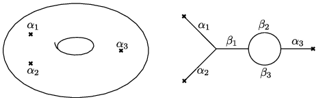
Under AGT relation, the conformal blocks are identified with Nekrasov’s partition function, and the product of with one-loop determinants. The momenta and correspond to masses and Coulomb branch parameters . In particular, each internal line in the Moore-Seiberg graph corresponds to an vector multiplet. With all these identifications understood, the formula (15) looks like an partition function [12].
Let us now look into the correspondence in more detail. First, it was proposed in [12] that the parameters of Omega deformation is related to the Liouville coupling as
| (16) |
This implies that the correspondence between Nekrasov’s partition functions and conformal blocks is for general Liouville central charge, but the partition function should correspond to Liouville correlators at a special (self-dual) value of Liouville coupling , since the Omega background with showed up near the poles. A natural question, as was already raised in [12], would have been what kind of deformation of would give the CFT correlators at . That led to the idea of squashing.
Second, the one-loop determinant in the partition function was identified with the product of the Liouville three-point function . The analytic property of can be determined from the following physical requirements of Liouville theory.
- •
is symmetric in its three arguments and invariant under .
- •
vanishes if one of takes value for degenerate Virasoro representations, .
- •
diverges if , since in this case the Liouville interaction can screen the violation of momentum conservation.
thus has several groups of poles and zeroes, each group containing infinite number of elements labelled by two nonnegative integers . These should be somehow related to the eigenvalues of .
The most interesting would have been the correspondence between conformal blocks and Nekrasov’s partition functions. In the traditional approach to CFT following [16], the only way to construct and study conformal blocks was via power series in 2D coordinate, or in other words summing up all the descendant operators appearing in the given operator product. There is actually a powerful recursion relations due to Zamolodchikov [19] that can determine the coefficients of higher terms in the series expansion from the lower ones, and it was used in prooving the AGT conjecture for some basic examples [20, 21]. A better understanding of conformal blocks beyond their definition as power series was definitely needed. This was a rather unexplored subject, although Liouville theory has a long history and has played such an important role in many places in string theory.
Liouville conformal blocks were studied from a different perspective in a series of work by Teschner [22, 23, 24, 25]. As we have seen, conformal blocks form a complete basis of solutions to conformal Ward identity in a given channel. One can therefore study the conformal blocks through their transformation property under changes of basis: namely how the bases of conformal blocks in different channels are related. Under AGT relation, different channel descriptions of the same correlator are in correspondence with different Lagrangian descriptions of the same 4D quantum field theory, that is the S-duality. On the other hand, it was known that the Liouville conformal blocks obey the same transformation rule under the change of basis as the wave functions in quantum Teichmüller theory, which is also related to quantization of the moduli space of flat gauge fields on punctured Riemann surface. In [26, 27] this fact was used as a key to explain how the 4D gauge theories and Liouville theory are related.
For later use, let us look at an example of basis-change of Liouville conformal blocks for one-point function on the torus. The corresponding Moore-Seiberg graph is a tadpole, and the conformal blocks are functions of the modulus of the torus as well the external and internal momenta . See Figure 2. They transform under modular S-transformation as follows,
| (17) |
Here we chose a different normalization of conformal blocks compared to (15). The integral kernel is known to take the following form [24],
| (18) | |||||
where is the double-sine function
| (19) |

3 3D gauge theories
The idea of SUSY localziation was applied to 3D supersymmetric Chern-Simons matter systems by Kapustin, Willett and Yaakov (KWY) [9]. Chern-Simons matter theories are a canonical example of 3D SCFTs, and some of them are known to have interpretations as theories of multiple M2-branes. Indeed, the original motivation of KWY was to provide a precise check of AdS/CFT through the explicit evaluation of Wilson loops. Moreover, their formula was also applied and gave an elegant solution to the long standing problem about the growth of the degree of freedom on multiple M2-branes. Their result also found applications and generalizations in many other interesting problems, some of which we review in the following.
partition function
KWY constructed supersymmetric Chern-Simons matter theories on and obtained closed formula for SUSY partition function as well as Wilson loop expectation values, which apply to a class of 3D supersymmetric systems. The system consists of two kinds of multiplets: a vector multiplet consists of a gauge field , gauginos , real scalar and an auxiliary scalar . Chiral multiplet consists of a complex scalar , fermion and a complex auxiliary scalar , and can couple to vector multiplet in arbitrary representation of the gauge group. The gauge fields have Chern-Simons kinetic term
| (20) |
where is the quantized Chern-Simons coupling. For each factor of the gauge group one can also turn on the Fayet-Iliopoulos coupling . For chiral multiplets, in addition to standard gauge interactions one can turn on other interactions through superpotential, or turn on the so-called real mass through gauging global symmetry. The supersymmetric Lagrangian and transformation rules can be written down based on the existence of conformal Killing spinors on ,
| (21) |
An important restriction, to which we will come back later, is that all the chilal multiplets here are assigned canonical R-charge 1/2.
The exact partition function depends on (convenient notation for the gauge group and its Chern-Simons coupling), and chiral matter representation . The formula reads
| (22) |
where
| (23) |
The FI coupling shows up as a modification of the integrand by [28].
With SUSY localization, the path integral can be shown to simplify to a finite-dimensional integral over constant values of vector multiplet scalar , which one can further restrict to the Cartan subalgebra. An important simplification compared to the four-dimensional case is the absence of saddle points with non-trivial topological quantum numbers such as instantons. Another simplification is that the one-loop determinant here can be evaluated explicitly as a product of eigenvalues using spherical harmonics, and the evaluation essentially boils down to representation theory of . Their formula is thus very easy to reproduce, so in a sense the 3D theories on can be thought of as an ideal exercise to learn the essence of SUSY localization.
Application to M2-brane theories
An important application of KWY formula is to the multiple M2-brane dynamics and /CFT3 correspondence. In this area, a long standing problem was how to understand the growth of the degrees of freedom (or free energy) on coincident M2-branes predicted by dual supergravity description. If the worldvolume theory on a stack of M2-branes is described by a 3D gauge theory with matrix valued fields, then the naive count of the degrees of freedom would be . The description of multiple M2-branes worldvolume theory itself was a long standing problem, but in [29] a superconformal Chern-Simons theory with bi-fundamental matters was proposed for M2-branes on orbifold . Indeed, it is a theory of matrix valued fields, while the dual supergravity predicts the large behavior for the free energy
| (24) |
An elegant solution for this mismatch was proposed in [30] by applying the traditional methods of large- matrix integrals to the partition function of ABJM model. They in particular found that the standard ’t Hooft expansion of the logarithm of sphere partition function reproduces (24) in its leading order. The subleading contributions as well as instanton contributions were studied in detail using various approaches to evaluate the integral (22), and interpreted in the dual picture. See the review [31] for more detail. Note that the fact that the partition function admits such an expansion or resummation is important in view of AdS/CFT correspondence. The observables in the gauge theory side need to have well defined analytic continuation in , because is mapped to cosmological constant in the gravity side.
AGT relation in 3D
In 4D gauge theories, one can introduce various defects and study them. According to their dimensionality they are called loops, surface defects, or domain walls (or boundaries). It is especially interesting to study how to describe them using lower dimensional field theories, or how the duality in 4D gauge theories act on them. Certain domain walls in 4D supersymmetric gauge theories are described by 3D field theories, and the sphere partition function gives an important information on their property.
The study of domain walls and boundaries for this purpose was started in SYM by Gaiotto and Witten [32, 33]. They were particularly interested in how the Montonen-Olive duality of the SYM acts on the boundaries and domain walls. As an example, consider the SYM with gauge group and take a half-BPS completion of Dirichlet boundary condition on gauge field. Its S-dual was then shown to be a 3D SCFT called on the boundary coupled to the bulk SYM with the S-dual gauge group . The theory is characterized by its global symmetry where is the gauge group for the S-dual theory. For , the wall theory has the 3D quiver description as in Figure 3.

For example, is the SQED with two charged hypermultiplets. A copy of acts as flavor rotation, while another isometry shows up as the isometry of the Coulomb branch moduli space in the infrared. The theory can also be used to describe the S-duality domain wall, that is the interface where the two SYM theory with gauge groups and are adjoined.
The structure of S-duality should be even richer for supersymmetric theories. As reviewed in the previous section, two mutually S-dual theories are related in the same way as the conformal blocks in two different channels are related. Then what kind of 3D theory shows up at the joint of a pair of mutually S-dual theories? Though general construction of such theories were not available, it was conjectured in [34] that the partition function of the theory on the wall should correspond to the transformation coefficients of conformal blocks under changes of channels, such as the example (18).
An attempt to see the correspondence was made in [35], which studied the S-duality wall between two 4D half-spaces both supporting theory with . The fields on the two sides are connected across the wall via S-duality. The vacua on the two sides are specified by two Coulomb branch parameters . The theory on the wall was identified as a suitable mass deformation of the theory explained above. In 3D terminology, it consists of a vector multiplet, two chiral multiplets of charge , two chirals of charge and a neutral chiral . The chiral matters all acquire mass proportional to the bulk mass-deformation . In addition, the parameters enter the theory as the FI parameter and the mass for charged chirals.
When computing the partition function for the wall theory, a small but nontrivial problem arose. The neutral chiral multiplet of the wall theory is assigned the R-charge 1, for which the one-loop determinant was not derived. Without knowing the contribution from it was proposed in the first version of [35]
| (25) | |||||
Though the analysis was incomplete, this result shows quite an agreement with (18). Thus it was proposed that the AGT relation can be generalized to include domain walls, and there is a precise relation between 3D gauge theories and 2D CFTs.
The above observation of the correspondence between 3D gauge theories and 2D CFTs was soon generalized in an interesting manner. To explain it, let us recall that the S-duality domain walls are closely related to Janus domain walls connecting the same 4D gauge theories at different values of coupling. As a generalization of Janus wall, let us consider the situation in which the gauge coupling varies smoothly as a function of one of the spatial coordinates, say . For theories of class S, the situation corresponds to M5-branes wrapping some Riemann surface whose shape varies as a function of . One can reinterpret it as M5-branes wrapping a 3-manifold. This picture leads to a correspondence between the geometry of hyperbolic 3-manifolds and the corresponding 3D gauge theories , as proposed in [36]. Moreover, a correspondence which is similar to AGT relation was proposed between observables of and Chern-Simons path integrals on [37, 38, 36, 39], and various precise correspondence have been reported.
Generalization of KWY formula
On a closer look at the formulae (18) and (25), it is tempting to identify with the one-loop determinant of the neutral chiral multiplet, as was proposed in the second version of [35]. It is also tempting to look for deformations of the round which reproduces the double sine function for general , as we will discuss in the next section.
Finding out the one-loop determinant arising from of non-canonical R-charge assignment requires generalizing the construction of supersymmetric theories on accordingly. This turned out possible, and what is intriguing was that the supersymmetry transformation rule for chiral multiplet then depends explicitly on its R-charge .
| (26) |
Similar R-charge dependence also shows up in the Lagrangian. The SUSY localization computation of partition function goes through, and the one-loop determinant for chiral multiplet of R-charge was found to be
| (27) |
generalizing (23). One can check using this formula that the neutral chiral multiplet of mass , R-charge 1 gives rise to the determinant which completes the agreement. This was reported by Jafferis [40], and one day later by [41].
F-theorem
Thanks to the above generalization, arbitrary supersymmetric theories with R-symmetry can now be put on preserving rigid supersymmetry. For theories with abelian global symmetry, the assignment of R-charges to chiral matters is not unique; any two consistent assignments , and , differ by a linear combination of abelian global symmetry charges . Given a reference R-charge , one can parametrize different assignments of R-charges in the following way,
| (28) |
The partition function then becomes a function of the parameters .
If the theory flows to a superconformal field theory in the infrared, then the R-symmetry in the IR limit is uniquely defined as a member of the superconformal algebra. Jafferis [40] made an interesting proposal that the corresponding value of can be determined by extremizing the real part of free energy . This was proved in [42] based on a careful study of the structure of couplings between current supermultiplets of the field theory and the background supergravity multiplet.
4 Squashing
The comparison of the formulae (18) and (25) leads to another natural guess that the partition function should be deformed in some way to reproduce the quantities in Liouville theory with . We encountered the same unsatisfactory situation also in the comparison of 4D and 2D observables, but the deformation of gauge theories seems easier to find.
It turned out that the rigid supersymmetry can be realized on manifolds less symmetric than the round sphere, and moreover one can derive exact formulae for supersymmetric observables on such manifolds. The important examples are squashed spheres. It was shown that for a suitable deformation of the the formula (22) is modified to exhibit the expected dependence.
Ellipsoid partition function
One way to achieve is to deform the round sphere into ellipsoid [43],
| (29) |
and generalize the Killing spinor equation to include a background gauge field ,
| (30) |
The scalar function and the gauge field are suitably chosen so that the above equations have solutions. Then the SUSY localization leads to the following formula for partition function,
| (31) |
which generalizes (22). The Liouville coupling was shown to be related to the axis-lengths by .
Sketch of derivation
The idea of ellipsoidal deformation naturally comes about from the following observation. In Pestun’s derivation of partition function, one-loop determinants were evaluated be relating it to the determinant of the bosonic symmetry on some reduced space of wavefunctions. It is reasonable to expect that play similar role in three dimensions as well. On the round sphere , the localization analysis was based on the Killing spinor satisfying
where are the generators of rotations of . This choice of Killing spinor is essentially unique due to the isometry of . Then a natural guess is that, if there were deformations of the sphere for , the square of the corresponding SUSY should be deformed in the following way,
| (32) |
The deformed geometry therefore should be symmetric, and ellipsoids (29) with the identification is an natural guess. However, at this level the idea is still too crude, because the conformal Killing spinor equation (30) was known to have solutions only on rather restricted class of manifolds. Indeed, one can try to solve (30) with various symmetric ansatz for the metric and see none of such attempts work except for the round sphere.
During the process of trial and error, we got interested in how the Killing spinor equation on the round would break down by small deformations of metric while keeping the Killing spinor unchanged. Since the problem is to find a family of geometry parametrized by , one can work perturbatively near . If the small deformation to the geometry were suitably chosen, we could fix the failure of Killing spinor equation somehow by modifying the Killing spinor accordingly. As the first experiment, the deformation of the round sphere into what was traditionally called squashed sphere was considered.
| (33) |
Here is the basis of left-invariant one-forms of . For a suitable choice of Killing spinor on the round sphere, the failure after deformation turned out to be
| (34) |
The original plan was to modify so that the failure term (RHS) disappears, but the above equation seemed to suggest a much nicer alternative solution. One can just regard the failure term as a coupling to a background vector field and include it into the covariant derivative.
It is a tedious but pleasant exercise to check that the construction of SUSY transformation rule and Lagrangians all goes through, under the assumption that are assigned the -charge . In particular, all the fields can be shown to couple to according to their R-charge in (26), thus can really be identified as the gauge field for R-symmetry. At this point, however, we were not sure what kind of framework would naturally accommodate this external gauge field. The external gauging of R-symmetry was regarded just as a tool to define supersymmetry on curved space, in a similar way to topological twisting.
There was no particular reason to consider the deformation to traditional squashed sphere (33), but in this way one is left with a large isometry unbroken. The spectrum on this space can therefore be explicitly solved using spherical harmonics. In some old literature there are even explicit results on related problems [44]. After a detailed spectrum analysis, we found that the eivenfunctions can be written using spherical harmonics in the same way as for the round sphere, but the degeneracy of eigenvalues gets partially resolved due to squashing. We were hoping that this broken degeneracy would lead to something new. But dissapointingly, the one-loop determinants stayed essentially the same as those for the round sphere.
After all, the square of supersymmetry on the traditional squashed sphere does not show the expected dependence on (32). Also, the eigenmodes turned out to make nontrivial contribution to the one-loop determinant as multiplets of the unbroken isometry, so that the determinant still has degeneration of many zeroes and poles. Thus it looked inevitable to break the isometry further and try seriously the ellipsoid (29).
Coming back from disappointment, it was pleasing to see that the ellipsoid (29) also admits charged Killing spinors if a suitable background gauge field is turned on. Moreover, this time the bilinear of Killing spinors indeed showed the expected -dependence (32). The only remaining problem was how to compute one-loop determinants.
On the ellipsoid (29) there seemed to be no easy way to solve the full spectrum. On the other hand, it was clear from previous experiences of determinant computations that most eigenmodes form bose-fermi pairs and do not make nontrivial contribution. It is therefore enough to know the spectrum of the remaining “unpaired modes”. It seemed difficult to translate our problem completely mathematically into the computation of an index as in [6]. Instead, in [43] the problem was studied in an equivalent and a little more physical approach by asking the following questions
- •
what are the Laplace and Dirac operators one wish to know the eigenvalues of.
- •
what is the map between the Laplace and Dirac eigenmodes for the same eigenvalue.
The one-loop determinant can then be expressed by collecting the eigenvalues of those unpaired modes which are sitting in the kernel and cokernel of the map. It turned out that all the unpaired modes can be easily listed up as solutions to some simple first-order differential equations. We thus arrived at an analytic result (31) which shows precisely the expected dependence on a new parameter .
Relation to superconformal index
It was noticed in [47, 48] that the 3D partition functions for theories have structures similar to superconformal indices for 4D theories. See [49] for a review. The superconformal index is an observable which encodes the spectrum of BPS operators, and is usually defined as the trace of time evolution operators over Hilbert space with an additional insertion of . Alternatively, one can use path integral formulation and define it as a partition function on with SUSY-preserving periodic periodicity condition on fields. The relation between 3D partition functions and 4D indices were studied from this viewpoint in [50].
One can introduce a one-parameter deformation to the 4D superconformal index which is similar to the squashing of 3D partition function by twisting the periodicity of fields along by isometry rotation of . Interestingly, if the 4D theory with this twist is dimensionally reduced, the resulting 3D theory is actually on the traditional squashed sphere (33), somewhat against our previous observation which led to the ellpsoid partition function. This led Imamura and Yokoyama to find another supersymmetric deformation of the round by introducing a background vector field [51].
Further generalization and supergravity
It is natural to ask what other three-manifolds admits rigid supersymmetry, and what is the maximim consistent generalization of the Killing spinor equation. Festuccia and Seiberg [52] proposed that the most suitable framework for such a study is off-shell supergravity. The background fields introduced in (30) or in [51] are then most naturally interpreted as the (auxiliary) fields in the gravity multiplet, and the Killing spinor equation is identified with the vanishing of local SUSY transformation of gravitino. Regarding the existence of rigid supersymmetry on curved space, it was shown that a 3D space admits a Killing spinor if it has an almost contact metric structure [53, 54]. The general theory of how the 3D partition function can depend on moduli of almost contact metric structure (such as the squashing parameter ) was developed in [55]. In particular, it was shown that partition function on three-manifolds of the topology of cannot depend on more than one squashing parameters [56].
Squashing
After an instructuve detour to three-dimensions, we finally came back to the problem of finding a deformation of which reproduces Liouville correlators with . A natural answer was proposed in [14] based on the 4D ellipsoid geometry
| (35) |
with some auxiliary fields in 4D off-shell supergravity turned on. Let us now sketch how this result was derived.
The first step was to identify correct generalization of Killing spinor equation (7), and then use it to construct the transformation rule and Lagrangian. This analysis was started before the observation of Festuccia and Seiberg [52], so the usefulness of supergravity was not recognized yet. So the only idea to generalize the Killing spinor equation (7) was to turn on R-symmetry gauge fields. Concerning the metric on the 4D manifold that realizes , it seemed natural to assume a fibration structure in which a 3D ellipsoid is fibered over a segment, with the fiber size shrinking at the two ends. The ellipsoid (35) is clearly one of such examples, where is the coordinate on the base segment and a 3D ellipsoid of varying size is fibered over it.
It was contrary to our optimistic expectations and even surprising that the ellipsoid does not admit Killing spinors no matter how one chooses the R-symmetry gauge field. After a more systematic study of the ellipsoid-fibration geometries, one 4D metric was found to admit Killing spinors, but it turned out to have rather strange singularity at the two poles (points at the end of the segment). It seemed somewhat awkward to discuss the physics of point-like instantons localized on such a singular point.
The first nontrivial step was made by recalling that near the north pole the Killing spinor of our interest should represent the SUSY of topologically twisted theory on Omega background . There the chiral part of Killing spinor vanishes while the anti-chiral part is finite. By a suitable gauge rotation one may set at the north pole, since in topologically twisted theory one identifies dotted spinor indices and R-symmetry indices. We also need that the square of the SUSY give rise to a rotation about the origin generated by the vector field
| (36) |
where are local Cartesian coordinates near the north pole. This determines the linear dependence of on coordinates
| (37) |
Now let us perform the failure term analysis in a similar way as in 3D case. On a flat without background gauge fields, the Killing spinor satisfies
| (38) |
Here , and the suffix indicates the self-dual or anti-self-dual components of two-forms. The failure term is in the second equation, the second term in the LHS. the tensor has nonvanishing components , and it vanishes near the north pole if the squashing deformation is turned off, . The above failure term seemed to suggest a rather unexpected form of generalized Killing spinor equation,
| (39) |
which involves an anti-self-dual tensor and a self-dual tensor auxiliary fields in addition to the R-symmetry gauge fields in .
It was an enjoyable, though tedious, exercise to construct the transformation rule and Lagrangian based on the above generalized Killing spinor equation. One complication was that one needs to require another set of equations on Killing spinor,
| (40) |
with another auxiliary field. This looked strange, since this kind of equations involving square of Dirac operator is usually automatically satisfied under the assumption of the first-order equations (39).
The proposal of Festuccia and Seiberg came out a little later. The generalized form (39) of Killing spinor equation turned out all consistent with the off-shell supergravity literature [57, 58], and the fields were identified with the auxiliary fields in gravity multiplet. Also, the additional Killing spinor equation (40) was identified with the local SUSY transformation rule of an auxiliary spin-1/2 fermion in gravity multiplet, thereby explaining why the two sets of equations (39) and (40) are independent.
The toughest part of the analysis was to show that the ellipsoid (35) indeed has Killing spinor for a suitable choice of background auxiliary fields. The strategy of [14] was to assume that a suitably chosen Killing spinor on the round remains a solution to the Killing spinor equation after squashing. This requirement turns the Killing spinor equation into a set of algebraic equations on the background supergravity fields. They looked highly overdetermined, but turned out to have a family of solutions which depends on three arbitrary functions invariant under isometry. See [14] for the explicit form of auxiliary fields. Thus the ellipsoid (35) was finally shown to admit rigid supersymmetry.
SUSY localization on
The SUSY localization analysis on the ellipsoid [14] begins by arguing, based on the continuity in the squashing parameter , that the SUSY saddle points are parametrized by a constant in the same way as on the round . Strictly speaking this assumption should be verified. For the case of 3D squashing the saddle-point analysis was fully carefully performed in [56]. Anyway, once this point is settled, the rest of the analysis is a straightforward application of localization program.
Again, at all the saddle points the gauge field have to vanish on generic points on the ellipsoid, but it is allowed to have point-like instanton or anti-instanton configurations at the two poles. Moreover, the theory approach near the poles the topologically twisted theory on with two independent Omega-deformation parameters .
Let us finally quickly summarize the essence of one-loop determinant computation and how it can be reduced to the computation of index. The computation of one-loop determinant involves a Gaussian integral over all the fluctuation modes at a give saddle point. Generally, one can choose as path integration variables a set of bosonic fields , a set of fermionic fields and their superpartners , . The supersymmetric measure is then
| (41) |
The one-loop determinant is evaluated as an integral with any -exact Gaussian weight . Let us take
| (42) | |||||
Then the one-loop determinant is simply the square root of the ratio of determinants of ,
| (43) |
It is instructive to see how all these work in examples with finite number of integration variables. In the toy example of the volume of sphere (1), the supersymmetry acts on the local coordinates , near the north pole as
| (44) |
The above formula can be used to explain the determinant at the north pole.
Application of this idea to the path integral of supersymmetric field theories involves renaming of fields. For example, 4D vector multiplet consists of 10 bosons and 10 fermions after gauge fixing: the physical fields , ghosts and Lautrup-Nakanishi field . We take as a combination of supersymmetry for a specific choice of Killing spinor and BRST symmetry, and reorganize these fields under its action. For example, gauge field is a member of the set whereas its superpartner
| (45) |
is a member of . The 10+10 fields are thus divided into four groups each consisting of five fields.
The ratio of determinant (43) can be further simplified if acting on the fields and has common eigenvalues. Especially if there is a differential operator which relates the fields to and commutes with , then the ratio of determinants can be computed from the index
| (46) | |||||
Note that the operator is in principle arbitrary as long as it commutes with , and it does not neccesarily have to be related to Lagrangian of the field theory. At this point, a powerful localization theorem in mathematics says the index can be computed as a sum over contributions from -fixed points, so we need the precise form of only near the poles. The reason of this localization is that involves a finite rotation (diffeomorphism). If it acts on coordinates as , then the trace of such operator should involve an integral of delta function,
| (47) |
so it localizes onto fixed points. For more details see [6, 14] as well as reviews [59, 60].
5 Concluding remarks
Let us briefly mention on the progress in other dimensions. In five dimensions, the sphere partition function for supersymmetric gauge theories was studied in [61, 62, 63, 64, 65, 66, 67, 68, 69]. There the important problem was to see how the sphere partition functions for maximally supersymmetric SYM are related to the index of 6D (2,0) superconformal theories, and to read off the large- scaling of the degrees of freedom on coincident M5-branes . In two dimensions, the sphere partition function for gauge theories was studied in [70, 71, 72]. In particular, for those which flow to superconformal field theories, it was shown that the sphere partition function computes directly the Kähler potential for the moduli space of superconformal theories.
Localization techniques have been applied to the evaluation of many supersymmmetric obsercables. In addition to partition functions, various non-local observables such as Wilson loop ’t Hooft loops, surface operatrors has neen also studied using this technique. They are not only playing important roles in understanding mathematical structures underlying supersymmetric gauge theories, but also help us understanding better how to define and compute such operators precisely within path integral formalism.
Acknowledgment
The author would like to thank Naofumi Hama, Sungjay Lee and Jaemo Park for collaboration on the materials reviewed in this article. The author is also gratedul to the Elementary Particle Physics Group at Tokyo Institute of Technology for giving him opportunity to review the developments in Liouville theory.
References
- [1] Edward Witten, J.Geom.Phys., 9, 303–368 (1992), arXiv:hep-th/9204083.
- [2] Edward Witten, Commun.Math.Phys., 117, 353 (1988).
- [3] Edward Witten, Commun.Math.Phys., 118, 411 (1988).
- [4] Nikita A. Nekrasov, Adv.Theor.Math.Phys., 7, 831–864 (2004), arXiv:hep-th/0206161.
- [5] Hiroshi Itoyama (review in the same volume).
- [6] Vasily Pestun, Commun.Math.Phys., 313, 71–129 (2012), arXiv:0712.2824.
- [7] J.K. Erickson, G.W. Semenoff, and K. Zarembo, Nucl.Phys., B582, 155–175 (2000), arXiv:hep-th/0003055.
- [8] Nadav Drukker and David J. Gross, J.Math.Phys., 42, 2896–2914 (2001), arXiv:hep-th/0010274.
- [9] Anton Kapustin, Brian Willett, and Itamar Yaakov, JHEP, 1003, 089 (2010), arXiv:0909.4559.
- [10] Seok Kim, Nucl.Phys., B821, 241–284 (2009), arXiv:0903.4172.
- [11] Davide Gaiotto, JHEP, 1208, 034 (2012), arXiv:0904.2715.
- [12] Luis F. Alday, Davide Gaiotto, and Yuji Tachikawa, Lett.Math.Phys., 91, 167–197 (2010), arXiv:0906.3219.
- [13] Niclas Wyllard, JHEP, 0911, 002 (2009), arXiv:0907.2189.
- [14] Naofumi Hama and Kazuo Hosomichi, JHEP, 1209, 033 (2012), arXiv:1206.6359.
- [15] Yuji Tachikawa (review in the same volume).
- [16] A.A. Belavin, Alexander M. Polyakov, and A.B. Zamolodchikov, Nucl.Phys., B241, 333–380 (1984).
- [17] Harald Dorn and H.J. Otto, Nucl.Phys., B429, 375–388 (1994), arXiv:hep-th/9403141.
- [18] Alexander B. Zamolodchikov and Alexei B. Zamolodchikov, Nucl.Phys., B477, 577–605 (1996), arXiv:hep-th/9506136.
- [19] A.B. Zamolodchikov, Commun.Math.Phys., 96, 419–422 (1984).
- [20] V.A. Fateev and A.V. Litvinov, JHEP, 1002, 014 (2010), arXiv:0912.0504.
- [21] Leszek Hadasz, Zbigniew Jaskolski, and Paulina Suchanek, JHEP, 1006, 046 (2010), arXiv:1004.1841.
- [22] J. Teschner, Fortsch.Phys., 51, 865–872 (2003), arXiv:hep-th/0212243.
- [23] J. Teschner, Int.J.Mod.Phys., A19S2, 459–477 (2004), arXiv:hep-th/0303149.
- [24] J. Teschner (2003), arXiv:hep-th/0308031.
- [25] J. Teschner (2005), arXiv:math/0510174.
- [26] Nikita Nekrasov and Edward Witten, JHEP, 1009, 092 (2010), arXiv:1002.0888.
- [27] G. Vartanov and J. Teschner (2013), arXiv:1302.3778.
- [28] Anton Kapustin, Brian Willett, and Itamar Yaakov, JHEP, 1010, 013 (2010), arXiv:1003.5694.
- [29] Ofer Aharony, Oren Bergman, Daniel Louis Jafferis, and Juan Maldacena, JHEP, 0810, 091 (2008), arXiv:0806.1218.
- [30] Nadav Drukker, Marcos Marino, and Pavel Putrov, Commun.Math.Phys., 306, 511–563 (2011), arXiv:1007.3837.
- [31] Sanefumi Moriyama and Kazumi Okuyama (review in the same volume).
- [32] Davide Gaiotto and Edward Witten, J.Statist.Phys., 135, 789–855 (2009), arXiv:0804.2902.
- [33] Davide Gaiotto and Edward Witten, Adv.Theor.Math.Phys., 13, 721 (2009), arXiv:0807.3720.
- [34] Nadav Drukker, Davide Gaiotto, and Jaume Gomis, JHEP, 1106, 025 (2011), arXiv:1003.1112.
- [35] Kazuo Hosomichi, Sungjay Lee, and Jaemo Park, JHEP, 1012, 079 (2010), arXiv:1009.0340.
- [36] Tudor Dimofte, Davide Gaiotto, and Sergei Gukov, Commun.Math.Phys., 325, 367–419 (2014), arXiv:1108.4389.
- [37] Yuji Terashima and Masahito Yamazaki, JHEP, 1108, 135 (2011), arXiv:1103.5748.
- [38] Tudor Dimofte and Sergei Gukov, JHEP, 1305, 109 (2013), arXiv:1106.4550.
- [39] Tudor Dimofte, Davide Gaiotto, and Sergei Gukov, Adv.Theor.Math.Phys., 17, 975–1076 (2013), arXiv:1112.5179.
- [40] Daniel L. Jafferis, JHEP, 1205, 159 (2012), arXiv:1012.3210.
- [41] Naofumi Hama, Kazuo Hosomichi, and Sungjay Lee, JHEP, 1103, 127 (2011), arXiv:1012.3512.
- [42] Cyril Closset, Thomas T. Dumitrescu, Guido Festuccia, Zohar Komargodski, and Nathan Seiberg, JHEP, 1210, 053 (2012), arXiv:1205.4142.
- [43] Naofumi Hama, Kazuo Hosomichi, and Sungjay Lee, JHEP, 1105, 014 (2011), arXiv:1102.4716.
- [44] G.W. Gibbons, Annals Phys., 125, 98 (1980).
- [45] Nadav Drukker, Takuya Okuda, and Filippo Passerini, JHEP, 1407, 137 (2014), arXiv:1211.3409.
- [46] Kazuo Hosomichi (2014), arXiv:1412.7128.
- [47] F.A.H. Dolan, V.P. Spiridonov, and G.S. Vartanov, Phys.Lett., B704, 234–241 (2011), arXiv:1104.1787.
- [48] Abhijit Gadde and Wenbin Yan, JHEP, 1212, 003 (2012), arXiv:1104.2592.
- [49] Yosuke Imamura (review in the same volume).
- [50] Yosuke Imamura, JHEP, 1109, 133 (2011), arXiv:1104.4482.
- [51] Yosuke Imamura and Daisuke Yokoyama, Phys.Rev., D85, 025015 (2012), arXiv:1109.4734.
- [52] Guido Festuccia and Nathan Seiberg, JHEP, 1106, 114 (2011), arXiv:1105.0689.
- [53] Claudius Klare, Alessandro Tomasiello, and Alberto Zaffaroni, JHEP, 1208, 061 (2012), arXiv:1205.1062.
- [54] Cyril Closset, Thomas T. Dumitrescu, Guido Festuccia, and Zohar Komargodski, JHEP, 1305, 017 (2013), arXiv:1212.3388.
- [55] Cyril Closset, Thomas T. Dumitrescu, Guido Festuccia, and Zohar Komargodski, JHEP, 1401, 124 (2014), arXiv:1309.5876.
- [56] Luis F. Alday, Dario Martelli, Paul Richmond, and James Sparks, JHEP, 1310, 095 (2013), arXiv:1307.6848.
- [57] B. de Wit, J.W. van Holten, and Antoine Van Proeyen, Nucl.Phys., B167, 186 (1980).
- [58] B. de Wit, J.W. van Holten, and Antoine Van Proeyen, Nucl.Phys., B184, 77 (1981).
- [59] Vasily Pestun (2014), arXiv:1412.7134.
- [60] Kazuo Hosomichi (to appear).
- [61] Johan Kallen and Maxim Zabzine, JHEP, 1205, 125 (2012), arXiv:1202.1956.
- [62] Kazuo Hosomichi, Rak-Kyeong Seong, and Seiji Terashima, Nucl.Phys., B865, 376–396 (2012), arXiv:1203.0371.
- [63] Johan Kallen, Jian Qiu, and Maxim Zabzine, JHEP, 1208, 157 (2012), arXiv:1206.6008.
- [64] Hee-Cheol Kim and Seok Kim, JHEP, 1305, 144 (2013), arXiv:1206.6339.
- [65] J. Kallen, J.A. Minahan, A. Nedelin, and M. Zabzine, JHEP, 1210, 184 (2012), arXiv:1207.3763.
- [66] Yosuke Imamura, PTEP, 2013, 013B04 (2013), arXiv:1209.0561.
- [67] Yosuke Imamura (2012), arXiv:1210.6308.
- [68] Hee-Cheol Kim, Joonho Kim, and Seok Kim (2012), arXiv:1211.0144.
- [69] Hee-Cheol Kim, Seok Kim, Sung-Soo Kim, and Kimyeong Lee (2013), 1307.7660.
- [70] Francesco Benini and Stefano Cremonesi (2012), arXiv:1206.2356.
- [71] Nima Doroud, Jaume Gomis, Bruno Le Floch, and Sungjay Lee, JHEP, 1305, 093 (2013), arXiv:1206.2606.
- [72] Jaume Gomis and Sungjay Lee, JHEP, 1304, 019 (2013), arXiv:1210.6022.