跳到论文正文
W Papers独立论文阅读器 arXiv:1502.04443 论文正文 计算阅读时间 · 0%
引用这篇论文根据当前论文元数据生成,正式投稿前建议核对。


License: arXiv.org perpetual non-exclusive license
arXiv:1502.04443v1 [quant-ph] 16 Feb 2015
Abstract

In this contribution, we investigate the entanglement behavior of a composite system consists of two different dimensional subsystems in non-inertial frames. In particular, we consider a composite system of qubit(two-dimensional) subsystem, and qutrit, (three-dimensional) subsystem. The degree of entanglement is quantified for different cases, where it is assumed that the two-subsystems are simultaneously or non- simultaneously accelerated. The entanglement decays as the acceleration of any subsystem increases.In general, the decay rate of entanglement increases as the dimensional of the accelerated subsystem increases. These results could be important in building an accelerated quantum network consists of different dimensions nodes.

Keyword: non-inertial frames, Entanglement, acceleration.

Entanglement of simultaneous and non-simultaneous Accelerated Qubit-Qutrit systems
N. Metwally

1 Department of Mathematics, College of Science, Bahrain University, Bahrain

2Department of Mathematics, Faculty of Science, Aswan University, Aswan, Egypt

email:nmetwally@gmail.com, nmetwally@uob.edu.bh

Tel:00973 33237474,   Fax: 00973 17449145

1 Introduction

It is well known that, quantum correlations are the most important physical quantities that have many applications in the context of quantum information, communication and computations [1, 2, 3]. The behavior of entanglement between different systems has investigated for small and high dimensions systems [4]. However, the properties of systems which are consists of different dimensional subsystems have investigated in different ways. For example, the behavior of entanglement for a two-parameter class of qubit-qutrit system passes through dissipative channels has discussed by Wei et.al, [5]. Karat and Gedik [6] have discussed the quantum and classical correlation of qubit-qutrit systems in the presence of classical dephasing environment. The quantum correlation’s behavior of a qubit-qutrit system under the effect of dephasing and bit flip channels has investigated by Guo et. al., [7]. Moreover, X. Xiao [8] has investigated the possibility of protecting the quantum correlation of qubit-qutrit system by using weak measurement and reversal.

Recently, the behavior of entanglement in non-inertial frames has investigated for different dimensional systems. For example, Alsing et. al., [14] have discussed the decay of entanglement between two modes of a free Dirac field in a non-inertial frame. The correlation between two modes of Dirac fields in non-inertial frames have investigated by Wang et. al, [10]. The dynamics of a general two qubit system in non-inertial frame is investigated by Metwally [11]. The possibility of using an accelerated class of XX-state to perform quantum coding is discussed in [12]. Moreover, teleportation in non-inertial frame is discussed by several authors see for example ([13, 14, 15]).

However, for composite system which consists of different dimensions subsystems, there are some limited efforts have been done to study the entangled properties of these systems in non-inertial frames. The effect of global, collective, local and multilocal depolarizing noise on qutrit-qutrit states is studied by S. Khan and M. Khan [16]. The measurement induced disturbance for qubit-qutrit system in non-inertial frames under the effect of different noise channel has investigated by Hao and Lian-Fu [17]. The importance of this problem appears clearly in the the context of generating accelerated network. To clarify this task, assume that a source supplies randomly some users who located in different nodes with different dimensional states to generated entangled network [18]. So, may any two nodes of the same or different dimensions systems are connected. Then it is important to quantify the degree of entanglement to find the optimal connection. Therefor, we are motivated to consider a general class of qubit-qutrit system in non-inertial frame, where we assume that these subsystems simultaneous and non-simultaneous accelerated.

This manuscript is organized as follows: In Sec. 22, we define the general form of the suggested system. The final state of the system is obtained analytically when one or both subsystems are accelerated simultaneously or non- simultaneously. In Sec. 33, the survival of entanglement between the two subsystems is quantified by using the negativity as a measure of entanglement. Finally, the results are summarized in Sec. 44.

2 System and its evolution

In this contribution, it is assumed that we have a composite system, consists of qubit (A)(A) and qutrit (B)(B), is given in its general form. The evolution the final state of the qubit-qutrit (Qb​tQ_{bt} ) system is investigated for three different cases: (i) the subsystem (A)(A) (qubit) is accelerated while qutrit (B)(B) is in a rest,(ii) the subsystem (B)(B) (qutrit) is accelerated while the subsystem (A)(A) is in a rest, (iii) Both subsystems are accelerated. The general state of the qubit-qutrit system is given by,

ρQb​t=16{I2⊗I+3∑i=13siσi⊗I3+∑i=18tjτj⊗I3+∑i=13∑j=18ci​jσi⊗τj},\rho_{Q_{bt}}=\frac{1}{6}\Bigl\{I_{2}\otimes I{{}_{3}}+\sum_{i=1}^{3}s_{i}\sigma_{i}\otimes I_{3}+\sum_{i=1}^{8}t_{j}\tau_{j}\otimes I_{3}+\sum_{i=1}^{3}\sum_{j=1}^{8}c_{ij}\sigma_{i}\otimes\tau_{j}\Bigr\}, (1)

where I2I_{2} and I3I_{3} are the unit matrix of size 2×22\times 2 and 3×33\times 3 respectively, si=t​r​{ρQb​t​σi⊗I3},tj=t​r​{ρQb​t​I2⊗τj}s_{i}=tr\bigl\{\rho_{Q_{bt}}\sigma_{i}\otimes I_{3}\bigr\},\quad t_{j}=tr\bigl\{\rho_{Q_{bt}}I_{2}\otimes\tau_{j}\bigr\} are the Bloch vectors for the qubit and the qutrit respectively, i=1..3,j=1..8i=1..3,\quad j=1..8. The operators σi\sigma_{i} and τj\tau_{j} are the traceless hermitian generators of S​u​(2)Su(2) and S​u​(3)Su(3) respectively. The elements ci​j=t​r​{ρQb​t​σi⊗τj}c_{ij}=tr\bigl\{\rho_{Q_{bt}}\sigma_{i}\otimes\tau_{j}\bigr\}, represent the correlation matrix between the qubit (A)(A) and the qutrit (B)(B). In the computational basis 00, 11 and 22, the operators σi\sigma_{i} and τj\tau_{j} can be written as,

σ1\displaystyle\sigma_{1} =\displaystyle= |0⟩⟨1|+|1⟩⟨0|,σ2=i|0⟩⟨1|−|1⟩⟨0|),σ3=|1⟩⟨1|−|0⟩⟨0|,\displaystyle\bigl|0\bigr\rangle\bigl\langle 1\bigr|+\bigl|1\bigr\rangle\bigl\langle 0\bigr|,\quad\sigma_{2}=i\bigl|0\bigr\rangle\bigl\langle 1\bigr|-\bigl|1\bigr\rangle\bigl\langle 0\bigr|),\quad\sigma_{3}=\bigl|1\bigr\rangle\bigl\langle 1\bigr|-\bigl|0\bigr\rangle\bigl\langle 0\bigr|,
τ1\displaystyle\tau_{1} =\displaystyle= |0⟩​⟨1|+|1⟩​⟨0|,τ2=i⁡(|1⟩​⟨0|−|0⟩​⟨1|),τ3=|0⟩​⟨0|−|1⟩​⟨1|,\displaystyle\bigl|0\bigr\rangle\bigl\langle 1\bigr|+\bigl|1\bigr\rangle\bigl\langle 0\bigr|,\quad\tau_{2}=i(\bigl|1\bigr\rangle\bigl\langle 0\bigr|-\bigl|0\bigr\rangle\bigl\langle 1\bigr|),\quad\tau_{3}=\bigl|0\bigr\rangle\bigl\langle 0\bigr|-\bigl|1\bigr\rangle\bigl\langle 1\bigr|,
τ4\displaystyle\tau_{4} =\displaystyle= |0⟩​⟨2|+|2⟩​⟨0|,τ5=i⁡(|2⟩​⟨0|−⟨0||2⟩),τ6=|1⟩​⟨2|+|2⟩​⟨1|,\displaystyle\bigl|0\bigr\rangle\bigl\langle 2\bigr|+\bigl|2\bigr\rangle\bigl\langle 0\bigr|,\quad\tau_{5}=i(\bigl|2\bigr\rangle\bigl\langle 0\bigr|-\bigl\langle 0\bigr|\bigl|2\bigr\rangle),\quad\tau_{6}=\bigl|1\bigr\rangle\bigl\langle 2\bigr|+\bigl|2\bigr\rangle\bigl\langle 1\bigr|,
τ7\displaystyle\tau_{7} =\displaystyle= i⁡(|2⟩​⟨1|−|1⟩​⟨2|),τ8=(|0⟩​⟨0|+|1⟩​⟨1|−2|2⟩​⟨2|)/3.\displaystyle i(\bigl|2\bigr\rangle\bigl\langle 1\bigr|-\bigl|1\bigr\rangle\bigl\langle 2\bigr|),\quad\tau_{8}=(\bigl|0\bigr\rangle\bigl\langle 0\bigr|+\bigl|1\bigr\rangle\bigl\langle 1\bigr|-2\bigl|2\bigr\rangle\bigl\langle 2\bigr|)/\sqrt{3}. (2)

In the computational basis, |00⟩,|01⟩,|02⟩,|10⟩,|11⟩\bigl|00\bigr\rangle,\bigl|01\bigr\rangle,\bigl|02\bigr\rangle,\bigl|10\bigr\rangle,\bigl|11\bigr\rangle and |12⟩\bigl|12\bigr\rangle, the state (1) can be written as,

ϱ00,i​j\displaystyle\varrho_{00,ij} =\displaystyle= 𝒜ℓ1,ℓ1=1​…​6,ϱ01,i​j=𝒜ℓ2,ℓ2=7​…​12,\displaystyle\mathcal{A}_{\ell_{1}},\quad\ell_{1}=1...6,\quad\quad\varrho_{01,ij}=\mathcal{A}_{\ell_{2}},\quad\ell_{2}=7...12,\quad
ϱ02,i​j\displaystyle\varrho_{02,ij} =\displaystyle= 𝒜ℓ3ℓ3=13​…​18,ϱ10,i​j=𝒜ℓ4,ℓ4=19​…​24,\displaystyle\mathcal{A}_{\ell_{3}}\quad\ell_{3}=13...18,\quad\varrho_{10,ij}=\mathcal{A}_{\ell_{4}},\quad\ell_{4}=19...24,\quad
ϱ11,i​j\displaystyle\varrho_{11,ij} =\displaystyle= 𝒜ℓ5​1,ℓ5=25​…​30,ϱ12,i​j=𝒜ℓ6,ℓ6=31​…​36,\displaystyle\mathcal{A}_{\ell_{5}1},\quad\ell_{5}=25...30,\quad\varrho_{12,ij}=\mathcal{A}_{\ell_{6}},\quad\ell_{6}=31...36,\quad (3)

where i​j=00,01,02,10,11,12ij=00,01,02,10,11,12 and 𝒜ℓ,ℓ=1​…​36\mathcal{A}_{\ell},\ell=1...36 are given in the appendix (A). For example, the element ϱ00,00=𝒜1,ϱ00,01=𝒜2,ϱ02,02=𝒜15ϱ12,12=𝒜36\varrho_{00,00}=\mathcal{A}_{1},\quad\varrho_{00,01}=\mathcal{A}_{2},\quad\varrho_{02,02}=\mathcal{A}_{15}\quad\varrho_{12,12}=\mathcal{A}_{36} and so on.

Now we investigate the evolution of the Qb​tQ_{bt} state (1) in non-inertial frame when one or both of its subsystems are accelerated as following:

  1. 1.

    Only the qubit is accelertaed
    In this context, it is important to review the behavior of a particle in non-inertial frames. It has been shown that, in the inertial frames, Minkowsik coordinates (t,z)(t,z) are used to describe Dirac field, while in the uniformly accelerated case, Rindler coordinates (τ,x)(\tau,x) are more adequate. The relations between the Minkowski and Rindler coordinates are given by[13, 19],

    τ=r​t​a​n​h​(tz),x=t2−z2,\tau=r~tanh\left(\frac{t}{z}\right),\quad x=\sqrt{t^{2}-z^{2}}, (4)

    where −∞<τ<∞-\infty<\tau<\infty, −∞<x<∞-\infty<x<\infty and rr is the acceleration of the moving particle. The relations (4) describe two regions in Rindler’s spaces: the first region II for |t|<x|t|<x and the second region I​III for x<−|t|x<-|t|.

    A single mode kk of fermions and anti-fermions in Minkowski space is described by the annihilation operators ak​Ua_{kU} and b−k​Ub_{-kU} respectively. In terms of Rindler’s operators ( ck​R(I),d−k​L(I​I)c^{(I)}_{kR},d^{(II)}_{-kL}), the Minkowski operators can be written as [20, 21],

    ak​U\displaystyle a_{kU} =\displaystyle= cos⁡r​ck,R(I)−exp⁡(−i​ϕ)​sin⁡r​d−k,L(I​I),\displaystyle\cos rc^{(I)}_{k,R}-\exp(-i\phi)\sin rd^{(II)}_{-k,L},
    b−k​U†\displaystyle b^{\dagger}_{-kU} =\displaystyle= exp⁡(i​ϕ)​sin⁡r​ck,R(I)+cos⁡r​dk,L(I​I),\displaystyle\exp(i\phi)\sin rc^{(I)}_{k,R}+\cos rd^{(II)}_{k,L}, (5)

    where, t​a​n​r=e−π​ω​catan~r=e^{-\pi\omega\frac{c}{a}}, 0≤r≤π/0\leq r\leq\pi/4, aa is the acceleration such that 0≤a≤∞0\leq a\leq\infty, ω\omega is the frequency of the travelling qubits, cc is the speed of light, and ϕ\phi is an unimportant phase that can be absorbed into the definition of the operators [22]. The operators (5) mix a particle in region II and an anti particle in region I​III as,

    |0k⟩\displaystyle\bigl|0_{k}\bigr\rangle =\displaystyle= cos⁡r​|0k⟩I​|0−k⟩I​I+sin⁡r​|1k⟩I​|1−k⟩I​I,\displaystyle\cos r\bigl|0_{k}\bigr\rangle_{I}\bigl|0_{-k}\bigr\rangle_{II}+\sin r\bigl|1_{k}\bigr\rangle_{I}\bigl|1_{-k}\bigr\rangle_{II},
    |1k⟩\displaystyle\bigl|1_{k}\bigr\rangle =\displaystyle= ak†​|0k⟩=|1k⟩I​|0k⟩I​I.\displaystyle a^{\dagger}_{k}\bigl|0_{k}\bigr\rangle=\bigl|1_{k}\bigr\rangle_{I}\bigl|0_{k}\bigr\rangle_{II}. (6)

    Now, by using the initial state of the qubit-qutrit system ρQb​t\rho_{Q_{bt}} (1) and the operators (6), the final state in the first region II of the Rindler space can be written in the basis 00,01,02,10,1100,01,02,10,11 and 1212. The density operator is represented by a matrix of size 6×66\times 6. Its elements are given by,

    ρ00,00(q)\displaystyle\rho_{00,00}^{(q)} =\displaystyle= cq2​ϱ00,00,ρ00,01(q)=cq2​ϱ00,01,ρ00,02(q)=cq2​ϱ00,02,ρ00,10(q)=cq​ϱ00,10,\displaystyle c^{2}_{q}\varrho_{00,00},\quad\rho_{00,01}^{(q)}=c^{2}_{q}\varrho_{00,01},\quad\rho_{00,02}^{(q)}=c^{2}_{q}\varrho_{00,02},\quad\rho_{00,10}^{(q)}=c_{q}\varrho_{00,10},
    ρ00,11(q)\displaystyle\quad\rho_{00,11}^{(q)} =\displaystyle= cq​ϱ00,11,ρ00,12(q)=cq​ϱ00,12,ρ01,00(q)=cq2​ϱ01,00,ρ01,01(q)=cq2​ϱ01,01,\displaystyle c_{q}\varrho_{00,11},\quad\rho_{00,12}^{(q)}=c_{q}\varrho_{00,12},\quad\rho_{01,00}^{(q)}=c^{2}_{q}\varrho_{01,00},\quad\rho_{01,01}^{(q)}=c^{2}_{q}\varrho_{01,01},\quad
    ρ01,02(q)\displaystyle\rho_{01,02}^{(q)} =\displaystyle= cq2​ϱ01,02,ρ01,10(q)=cq​ϱ01,10,ρ01,11(q)=cq​ϱ01,11,ρ01,12(q)=cq​ϱ01,12,\displaystyle c^{2}_{q}\varrho_{01,02},\quad\rho_{01,10}^{(q)}=c_{q}\varrho_{01,10},\quad\rho_{01,11}^{(q)}=c_{q}\varrho_{01,11},\quad\rho_{01,12}^{(q)}=c_{q}\varrho_{01,12},
    ρ02,00(q)\displaystyle\rho_{02,00}^{(q)} =\displaystyle= cq2​ϱ02,00,ρ02,01(q)=cq2​ϱ02,01,ρ02,02(q)=cq2​ϱ02,02,ρ02,10(q)=cq​ϱ02,10,\displaystyle c^{2}_{q}\varrho_{02,00},\quad\rho_{02,01}^{(q)}=c^{2}_{q}\varrho_{02,01},\quad\rho_{02,02}^{(q)}=c^{2}_{q}\varrho_{02,02},\quad\rho_{02,10}^{(q)}=c_{q}\varrho_{02,10},\quad
    ρ02,11(q)\displaystyle\rho_{02,11}^{(q)} =\displaystyle= cq​ϱ02,11,ρ02,12(q)=cq​ϱ02,12,ρ10,00(q)=cq​ϱ10,00,ρ10,01(q)=cq​ϱ10,01,\displaystyle c_{q}\varrho_{02,11},\quad\rho_{02,12}^{(q)}=c_{q}\varrho_{02,12},\quad\rho_{10,00}^{(q)}=c_{q}\varrho_{10,00},\quad\rho_{10,01}^{(q)}=c_{q}\varrho_{10,01},\quad
    ρ10,02(q)\displaystyle\rho_{10,02}^{(q)} =\displaystyle= cq​ϱ10,02,ρ10,10(q)=sq2​ϱ00,00+ϱ10,10,ρ10,11(q)=sq2​ϱ00,01+ϱ10,11,\displaystyle c_{q}\varrho_{10,02},\quad\rho_{10,10}^{(q)}=s^{2}_{q}\varrho_{00,00}+\varrho_{10,10},\quad\rho_{10,11}^{(q)}=s^{2}_{q}\varrho_{00,01}+\varrho_{10,11},
    ρ10,12(q)\displaystyle\rho_{10,12}^{(q)} =\displaystyle= sq2​ϱ00,02+ϱ10,12,ρ11,00(q)=cq​ϱ11,00,ρ11,01(q)=cq​ϱ11,01,ρ11,02(q)=cq​ϱ11,02,\displaystyle s^{2}_{q}\varrho_{00,02}+\varrho_{10,12},\quad\rho_{11,00}^{(q)}=c_{q}\varrho_{11,00},\quad\rho_{11,01}^{(q)}=c_{q}\varrho_{11,01},\quad\rho_{11,02}^{(q)}=c_{q}\varrho_{11,02},\quad
    ρ11,10(q)\displaystyle\rho_{11,10}^{(q)} =\displaystyle= sq2​ϱ01,00+ϱ11,10,ρ11,11(q)=sq2​ϱ01,01+ϱ11,11,ρ11,12(q)=sq2​ϱ01,02+ϱ11,12,\displaystyle s^{2}_{q}\varrho_{01,00}+\varrho_{11,10},\quad\rho_{11,11}^{(q)}=s^{2}_{q}\varrho_{01,01}+\varrho_{11,11},\quad\rho_{11,12}^{(q)}=s^{2}_{q}\varrho_{01,02}+\varrho_{11,12},
    ρ12,00(q)\displaystyle\rho_{12,00}^{(q)} =\displaystyle= cq​ϱ12,00,ρ12,01(q)=cq​ϱ12,01,ρ12,02(q)=cq​ϱ12,02,ρ12,10(q)=sq2​ϱ02,00+ϱ12,10,\displaystyle c_{q}\varrho_{12,00},\quad\rho_{12,01}^{(q)}=c_{q}\varrho_{12,01},\quad\rho_{12,02}^{(q)}=c_{q}\varrho_{12,02},\quad\rho_{12,10}^{(q)}=s^{2}_{q}\varrho_{02,00}+\varrho_{12,10},\quad
    ρ12,11(q)\displaystyle\rho_{12,11}^{(q)} =\displaystyle= sq2​ϱ02,01+ϱ12,11,ρ12,12(q)=sq2​ϱ02,02+ϱ12,12,\displaystyle s^{2}_{q}\varrho_{02,01}+\varrho_{12,11},\quad\rho_{12,12}^{(q)}=s^{2}_{q}\varrho_{02,02}+\varrho_{12,12}, (7)

    where cq=cos⁡rqc_{q}=\cos r_{q} and sq=s​i​n​rqs_{q}=sinr_{q}.

  2. 2.

    Only the qutrit is accelerated
    In this case, it is assumed that the qubit is in an inertial frame, while the qutrit undergoes a constant acceleration. For the two level qubit system (spin 1/21/2) particles, the Pauli-principle allows only two occupation numbers i.e.,”0” and ”1” [14]. However, the possibility of allowing the occupation number "​2​""2" is discussed by Leo`\grave{o}n and Marti`\grave{i}nez [23]. Under the single mode-approximation, Minlowaski vacuum state |0M⟩\bigl|0_{M}\bigr\rangle in the Rindler space reads as,

    |0M⟩=c​o​s2​r​|0⟩I​|0⟩I​I+ei​ϕ​sin⁡r​cos⁡r⁡(|𝒰⟩I​|𝒟⟩I​I+|𝒟⟩I​|𝒰⟩I​I)+e2​i​ϕ​s​i​n2​r​|𝒟⟩I​|𝒫⟩I​I,\bigl|0_{M}\bigr\rangle=cos^{2}r\bigl|0\bigr\rangle_{I}\bigl|0\bigr\rangle_{II}+e^{i\phi}\sin r\cos r(\bigl|\mathcal{U}\bigr\rangle_{I}\bigl|\mathcal{D}\bigr\rangle_{II}+\bigl|\mathcal{D}\bigr\rangle_{I}\bigl|\mathcal{U}\bigr\rangle_{II})+e^{2i\phi}sin^{2}r\bigl|\mathcal{D}\bigr\rangle_{I}\bigl|\mathcal{P}\bigr\rangle_{II}, (8)

    where |𝒰⟩,|𝒟⟩\bigl|\mathcal{U}\bigr\rangle,\bigl|\mathcal{D}\bigr\rangle and |𝒫⟩\bigl|\mathcal{P}\bigr\rangle are the spin up, spin down and pair state respectively. The spin up and down in Rindler space are given by,

    |𝒰M⟩\displaystyle\bigl|\mathcal{U}_{M}\bigr\rangle =\displaystyle= c​o​s​r​|𝒰⟩I​|0⟩I​I+ei​ϕ​sin⁡r​|𝒫⟩I​|𝒰⟩I​I,\displaystyle cosr\bigl|\mathcal{U}\bigr\rangle_{I}\bigl|0\bigr\rangle_{II}+e^{i\phi}\sin r\bigl|\mathcal{P}\bigr\rangle_{I}\bigl|\mathcal{U}\bigr\rangle_{II},
    |𝒟M⟩\displaystyle\bigl|\mathcal{D}_{M}\bigr\rangle =\displaystyle= c​o​s​r​|𝒟⟩I​|0⟩I​I−ei​ϕ​sin⁡r​|𝒫⟩I​|𝒟⟩I​I.\displaystyle cosr\bigl|\mathcal{D}\bigr\rangle_{I}\bigl|0\bigr\rangle_{II}-e^{i\phi}\sin r\bigl|\mathcal{P}\bigr\rangle_{I}\bigl|\mathcal{D}\bigr\rangle_{II}. (9)

    By using the initial state (1) and the transformation (8,9) one can obtain the final state of the accelerated system. After tracing out the mode in the second region I​III, we obtain the final accelerated state in the first region II of the Rindler space. In the basis, |ℓ,0⟩,|ℓ,𝒟⟩,|ℓ,𝒰⟩,|ℓ,𝒫⟩(ℓ=0,1)\bigl|\ell,0\bigr\rangle,\bigl|\ell,\mathcal{D}\bigr\rangle,\bigl|\ell,\mathcal{U}\bigr\rangle,\bigl|\ell,\mathcal{P}\bigr\rangle~(\ell=0,1), the density operator is defined by a matrix of size 8×88\times 8, where its elements are given by,

    ρ00,00(t)\displaystyle\rho^{(t)}_{00,00} =\displaystyle= ct4​ϱ00,00,ρ​(t)00,0​𝒟=ct3​ϱ00,01,ρ​(t)00,0​𝒰=ct2​ϱ00,02,ρ​(t)00,0​𝒫=0,\displaystyle c_{t}^{4}\varrho_{00,00},\quad\rho{(t)}_{00,0\mathcal{D}}=c_{t}^{3}\varrho_{00,01},\quad\rho{(t)}_{00,0\mathcal{U}}=c_{t}^{2}\varrho_{00,02},\quad\rho{(t)}_{00,0\mathcal{P}}=0,\quad
    ρ​(t)00,10\displaystyle\rho{(t)}_{00,10} =\displaystyle= ct4​ϱ00,10,ρ00,1​𝒟(t)=ct3​ϱ00,11,ρ00,1​𝒰(t)=ct2​ϱ00,12,ρ00,1​𝒫=0,ρ0​𝒟,00(t)=ct4​ϱ01,00,\displaystyle c_{t}^{4}\varrho_{00,10},\quad\rho^{(t)}_{00,1\mathcal{D}}=c_{t}^{3}\varrho_{00,11},\quad\rho^{(t)}_{00,1\mathcal{U}}=c_{t}^{2}\varrho_{00,12},\quad\rho_{00,1\mathcal{P}}=0,\quad\rho^{(t)}_{0\mathcal{D},00}=c_{t}^{4}\varrho_{01,00},\quad
    ρ0​𝒟,0​𝒟(t)\displaystyle\rho^{(t)}_{0\mathcal{D},0\mathcal{D}} =\displaystyle= ct2​(st2​ϱ00,00+ϱ01,01),ρ0​𝒟,0​𝒰(t)=ct2​ϱ01,02,ρ0​𝒟,0​𝒫=ct​st2​ϱ00,02,\displaystyle c_{t}^{2}(s^{2}_{t}\varrho_{00,00}+\varrho_{01,01}),\quad\rho^{(t)}_{0\mathcal{D},0\mathcal{U}}=c_{t}^{2}\varrho_{01,02},\quad\rho_{0\mathcal{D},0\mathcal{P}}=c_{t}s^{2}_{t}\varrho_{00,02},
    ρ0​𝒟,𝒟​0(t)\displaystyle\rho^{(t)}_{0\mathcal{D},\mathcal{D}0} =\displaystyle= ct4​ϱ01,10,ρ0​𝒟,𝒟​𝒟(t)=ct2​(st2​ϱ00,10+ϱ01,11),ρ0​𝒟,1​𝒰(t)=ct2​ϱ01,12,ρ0​𝒟,1​𝒫(t)=ct​st2​ϱ00,12,\displaystyle c_{t}^{4}\varrho_{01,10},\quad\rho^{(t)}_{0\mathcal{D},\mathcal{D}\mathcal{D}}=c^{2}_{t}(s^{2}_{t}\varrho_{00,10}+\varrho_{01,11}),\quad\rho^{(t)}_{0\mathcal{D},1\mathcal{U}}=c_{t}^{2}\varrho_{01,12},\quad\rho^{(t)}_{0\mathcal{D},1\mathcal{P}}=c_{t}s^{2}_{t}\varrho_{00,12},
    ρ0​𝒰,00(t)\displaystyle\rho^{(t)}_{0\mathcal{U},00} =\displaystyle= ct3​ϱ02,00,ρ02​𝒰,0​𝒟(t)=ct3​ϱ02,01,ρ0​𝒰,0​𝒰(t)=ct2​(st2​ϱ00,01+ϱ02,02),ρ0​𝒰,0​𝒫(t)=−ct​st2​ϱ02,10,\displaystyle c_{t}^{3}\varrho_{02,00},\quad\rho^{(t)}_{02\mathcal{U},0\mathcal{D}}=c_{t}^{3}\varrho_{02,01},\quad\rho^{(t)}_{0\mathcal{U},0\mathcal{U}}=c^{2}_{t}(s^{2}_{t}\varrho_{00,01}+\varrho_{02,02}),\quad\rho^{(t)}_{0\mathcal{U},0\mathcal{P}}=-c_{t}s^{2}_{t}\varrho_{02,10},\quad
    ρ0​𝒰,10(t)\displaystyle\rho^{(t)}_{0\mathcal{U},10} =\displaystyle= ct3​ϱ02,10,ρ0​𝒰,1​𝒟(t)=ct2​ϱ02,11,ρ0​𝒰,1​𝒰(t)=ct2​(st2​ϱ02,10+ϱ02,12),ρ0​𝒰,1​𝒫(t)=−ct​st2​ϱ00,11,\displaystyle c_{t}^{3}\varrho_{02,10},\quad\rho^{(t)}_{0\mathcal{U},1\mathcal{D}}=c_{t}^{2}\varrho_{02,11},\quad\rho^{(t)}_{0\mathcal{U},1\mathcal{U}}=c^{2}_{t}(s^{2}_{t}\varrho_{02,10}+\varrho_{02,12}),\quad\rho^{(t)}_{0\mathcal{U},1\mathcal{P}}=-c_{t}s^{2}_{t}\varrho_{00,11},\quad
    ρ0​𝒫,00(t)\displaystyle\rho^{(t)}_{0\mathcal{P},00} =\displaystyle= 0,ρ0​𝒫,0​𝒟(t)=ct​st2​ϱ02,00,ρ0​𝒫,0​𝒰(t)=−ct​st2​ϱ01,00,ρ0​𝒫,0​𝒫(t)=st2​(st2​ϱ00,00+ϱ01,02),\displaystyle 0,\quad\rho^{(t)}_{0\mathcal{P},0\mathcal{D}}=c_{t}s_{t}^{2}\varrho_{02,00},\quad\rho^{(t)}_{0\mathcal{P},0\mathcal{U}}=-c_{t}s_{t}^{2}\varrho_{01,00},\quad\rho^{(t)}_{0\mathcal{P},0\mathcal{P}}=s^{2}_{t}(s^{2}_{t}\varrho_{00,00}+\varrho_{01,02}),\quad
    ρ0​𝒫,10(t)\displaystyle\rho^{(t)}_{0\mathcal{P},10} =\displaystyle= 0,ρ0​𝒫,1​𝒟(t)=ct​st2​ϱ02,10,ρ0​𝒫,1​𝒰(t)=−ct​st2​ϱ01,10,ρ0​𝒫,1​𝒫(t)=st4​ϱ00,10,\displaystyle 0,\quad\rho^{(t)}_{0\mathcal{P},1\mathcal{D}}=c_{t}s_{t}^{2}\varrho_{02,10},\quad\rho^{(t)}_{0\mathcal{P},1\mathcal{U}}=-c_{t}s_{t}^{2}\varrho_{01,10},\quad\rho^{(t)}_{0\mathcal{P},1\mathcal{P}}=s_{t}^{4}\varrho_{00,10},
    ρ10,00(t)\displaystyle\rho^{(t)}_{10,00} =\displaystyle= ct4​ϱ10,00,ρ10,0​𝒟(t)=ct3​ϱ10,01,ρ10,0​𝒰(t)=ct2​ϱ10,02,ρ10,0​p(t)=0\displaystyle c^{4}_{t}\varrho_{10,00},\quad\rho^{(t)}_{10,0\mathcal{D}}=c^{3}_{t}\varrho_{10,01},\quad\rho^{(t)}_{10,0\mathcal{U}}=c^{2}_{t}\varrho_{10,02},\quad\rho^{(t)}_{10,0p}=0
    ρ10,10(t)\displaystyle\rho^{(t)}_{10,10} =\displaystyle= ct4​ϱ10,10,ρ10,1​𝒟(t)=ct3​ϱ10,11,ρ10,12​𝒰(t)=ct2​ϱ10,12,ρ10,1​𝒫(t)=0,\displaystyle c^{4}_{t}\varrho_{10,10},\quad\rho^{(t)}_{10,1\mathcal{D}}=c^{3}_{t}\varrho_{10,11},\quad\rho^{(t)}_{10,12\mathcal{U}}=c^{2}_{t}\varrho_{10,12},\quad\rho^{(t)}_{10,1\mathcal{P}}=0,
    ρ1​𝒟,00(t)\displaystyle\rho^{(t)}_{1\mathcal{D},00} =\displaystyle= ct3​ϱ11,00,ρ1​𝒟,0​𝒟(t)=ct2​ϱ11,01,ρ1​𝒟,0​𝒰(t)=ct2​ϱ11,02,ρ1​𝒟,0​𝒫(t)=ct​st2​ϱ10,02,\displaystyle c^{3}_{t}\varrho_{11,00},\quad\rho^{(t)}_{1\mathcal{D},0\mathcal{D}}=c^{2}_{t}\varrho_{11,01},\quad\rho^{(t)}_{1\mathcal{D},0\mathcal{U}}=c^{2}_{t}\varrho_{11,02},\quad\rho^{(t)}_{1\mathcal{D},0\mathcal{P}}=c_{t}s^{2}_{t}\varrho_{10,02},
    ρ1​𝒟,10(t)\displaystyle\rho^{(t)}_{1\mathcal{D},10} =\displaystyle= ct3​ϱ11,10,ρ1​𝒟,1​𝒟(t)=ct2​st2​ϱ11,11,ρ1​𝒟,1​𝒰(t)=ct2​ϱ11,12,ρ1​𝒟,1​𝒫(t)=ct2​st2​ϱ10,12,\displaystyle c^{3}_{t}\varrho_{11,10},\quad\rho^{(t)}_{1\mathcal{D},1\mathcal{D}}=c^{2}_{t}s^{2}_{t}\varrho_{11,11},\quad\rho^{(t)}_{1\mathcal{D},1\mathcal{U}}=c^{2}_{t}\varrho_{11,12},\quad\rho^{(t)}_{1\mathcal{D},1\mathcal{P}}=c^{2}_{t}s^{2}_{t}\varrho_{10,12},
    ρ1​𝒰,00(t)\displaystyle\rho^{(t)}_{1\mathcal{U},00} =\displaystyle= ct2​ϱ12,00,ρ1​𝒰,0​𝒟(t)=ct2​ϱ12,01,ρ1​𝒰,0​𝒰(t)=ct2​ϱ12,02,ρ1​𝒰,0​𝒫(t)=−ct​st2​ϱ10,01,\displaystyle c^{2}_{t}\varrho_{12,00},\quad\rho^{(t)}_{1\mathcal{U},0\mathcal{D}}=c^{2}_{t}\varrho_{12,01},\quad\rho^{(t)}_{1\mathcal{U},0\mathcal{U}}=c^{2}_{t}\varrho_{12,02},\quad\rho^{(t)}_{1\mathcal{U},0\mathcal{P}}=-c_{t}s^{2}_{t}\varrho_{10,01},
    ρ1​𝒰,10(t)\displaystyle\rho^{(t)}_{1\mathcal{U},10} =\displaystyle= ct2​ϱ12,10,ρ1​𝒰,1​𝒟(t)=ct2​ϱ12,11,ρ1​𝒰,1​𝒰(t)=ct2​st2​ϱ10,10,ρ1​𝒰,1​𝒫(t)=−ct2​st​ϱ10,112,\displaystyle c^{2}_{t}\varrho_{12,10},\quad\rho^{(t)}_{1\mathcal{U},1\mathcal{D}}=c^{2}_{t}\varrho_{12,11},\quad\rho^{(t)}_{1\mathcal{U},1\mathcal{U}}=c^{2}_{t}s^{2}_{t}\varrho_{10,10},\quad\rho^{(t)}_{1\mathcal{U},1\mathcal{P}}=-c^{2}_{t}s_{t}\varrho_{10,112},
    ρ1​𝒫,00(t)\displaystyle\rho^{(t)}_{1\mathcal{P},00} =\displaystyle= 0,ρ1​𝒫,0​𝒟(t)=ct2​st2​ϱ12,00,ρ1​𝒫,0​𝒰(t)=−ct​st2​ϱ11,00,ρ1​𝒫,0​𝒫(t)=st2​(ϱ11,01+ϱ12,02),\displaystyle 0,\quad\rho^{(t)}_{1\mathcal{P},0\mathcal{D}}=c^{2}_{t}s^{2}_{t}\varrho_{12,00},\quad\rho^{(t)}_{1\mathcal{P},0\mathcal{U}}=-c_{t}s^{2}_{t}\varrho_{11,00},\quad\rho^{(t)}_{1\mathcal{P},0\mathcal{P}}=s^{2}_{t}(\varrho_{11,01}+\varrho_{12,02}),
    ρ1​𝒫,10(t)\displaystyle\rho^{(t)}_{1\mathcal{P},10} =\displaystyle= 0,ρ1​𝒫,1​𝒟(t)=ct2​ϱ12,11,ρ1​𝒫,1​𝒰(t)=−ct​st2​ϱ11,10,ρ1​𝒫,1​𝒫(t)=st2​(ϱ11,12+ϱ12,12),\displaystyle 0,\rho^{(t)}_{1\mathcal{P},1\mathcal{D}}=c^{2}_{t}\varrho_{12,11},\quad\rho^{(t)}_{1\mathcal{P},1\mathcal{U}}=-c_{t}s^{2}_{t}\varrho_{11,10},\quad\rho^{(t)}_{1\mathcal{P},1\mathcal{P}}=s^{2}_{t}(\varrho_{11,12}+\varrho_{12,12}), (10)

    where ct=cos⁡rtc_{t}=\cos r_{t} and st=s​i​n​rts_{t}=sin~r_{t}.

  3. 3.

    Both subsystems are accelerated:
    In this case, we assume that both subsystems are accelerated. The final state of the system in the first region II of the Rindler space is defined by a matrix of size 8×88\times 8 elements. The elements of this matrix are given by,

    ρ00,j​k(q​t)\displaystyle\rho^{(qt)}_{00,jk} =\displaystyle= ℬℓ1(q​t),ℓ1=1..3,j​k=00,0​𝒟,0​𝒰,ρ00,j​k(q​t)=ℬℓ2,ℓ2=4,5,j​k=10,1​𝒟,\displaystyle\mathcal{B}^{(qt)}_{\ell_{1}},\quad\ell_{1}=1..3,\quad jk=00,0\mathcal{D},0\mathcal{U},\quad\rho^{(qt)}_{00,jk}=\mathcal{B}_{\ell_{2}},\quad\ell_{2}=4,5,\quad jk=10,1\mathcal{D},
    ρ00,12(q​t)\displaystyle\rho^{(qt)}_{00,12} =\displaystyle= ϱ00,1​𝒫=0,ρ01,j​k(q​t)=ℬℓ3,ℓ3=ℬ6…ℬ13,jk=00,0𝒟,0𝒰,0𝒫,10,1𝒟,1𝒰,1𝒫,\displaystyle\varrho_{00,1\mathcal{P}}=0,\quad\rho_{01,jk}^{(qt)}=\mathcal{B}_{\ell_{3}},\quad\ell_{3}=\mathcal{B}_{6}...\mathcal{B}_{13},\quad jk=00,0\mathcal{D},0\mathcal{U},0\mathcal{P},10,1\mathcal{D},1\mathcal{U},1\mathcal{P},\quad
    ρ02,j​k(q​t)\displaystyle\rho^{(qt)}_{02,jk} =\displaystyle= ℬℓ4,ℓ4=ℬ14​…​ℬ21,j​k=00,0​𝒟,0​𝒰,0​𝒫,10,1​𝒟,1​𝒰,1​𝒫,ρ0​𝒫,00(q​t)=ρ0​𝒫,10=0,\displaystyle\mathcal{B}_{\ell_{4}},\quad\ell_{4}=\mathcal{B}_{14}...\mathcal{B}_{21},\quad jk=00,0\mathcal{D},0\mathcal{U},0\mathcal{P},10,1\mathcal{D},1\mathcal{U},1\mathcal{P},\quad\rho^{(qt)}_{0\mathcal{P},00}=\rho_{0\mathcal{P},10}=0,\quad
    ϱ0​𝒫,j​k(q​t)\displaystyle\varrho^{(qt)}_{0\mathcal{P},jk} =\displaystyle= ℬℓ5,ℓ5=ℬ22​…​ℬ27,j​k=0​𝒟,0​𝒰,0​𝒫,1​𝒟,1​𝒰,1​𝒫ρ10,0​𝒫(q​t)=ρ10,1​𝒫(q​t)=0,\displaystyle\mathcal{B}_{\ell_{5}},\quad\ell_{5}=\mathcal{B}_{22}...\mathcal{B}_{27},\quad jk=0\mathcal{D},0\mathcal{U},0\mathcal{P},1\mathcal{D},1\mathcal{U},1\mathcal{P}\quad\rho^{(qt)}_{10,0\mathcal{P}}=\rho^{(qt)}_{10,1\mathcal{P}}=0,
    ρ10,j​k(q​t)\displaystyle\rho^{(qt)}_{10,jk} =\displaystyle= ℬℓ6,ℓ6=ℬ28​…​ℬ33,j​k=00,0​𝒟,0​𝒰,10,1​𝒟,1​𝒰,ρ11,00=0,\displaystyle\mathcal{B}_{\ell_{6}},\quad\ell_{6}=\mathcal{B}_{28}...\mathcal{B}_{33},\quad jk=00,0\mathcal{D},0\mathcal{U},10,1\mathcal{D},1\mathcal{U},\quad\rho_{11,00}=0,\quad
    ρ1​𝒟,j​k(q​t)\displaystyle\rho^{(qt)}_{1\mathcal{D},jk} =\displaystyle= ℬℓ7,ℓ7=ℬ34​…​ℬ40,j​k=0​𝒟,0​𝒰,0​𝒫,10,1​𝒟,1​𝒰,1​𝒫,\displaystyle\mathcal{B}_{\ell_{7}},\quad\ell_{7}=\mathcal{B}_{34}...\mathcal{B}_{40},\quad jk=0\mathcal{D},0\mathcal{U},0\mathcal{P},10,1\mathcal{D},1\mathcal{U},1\mathcal{P},
    ρ1​𝒰,j​k(q​t)\displaystyle\rho^{(qt)}_{1\mathcal{U},jk} =\displaystyle= ℬℓ8,ℓ8=ℬ41​…​ℬ48,j​k=00,0​𝒟,0​𝒰,10,1​𝒟,1​𝒰,1​𝒫,\displaystyle\mathcal{B}_{\ell_{8}},\quad\ell_{8}=\mathcal{B}_{41}...\mathcal{B}_{48},\quad jk=00,0\mathcal{D},0\mathcal{U},10,1\mathcal{D},1\mathcal{U},1\mathcal{P},
    ρ1​𝒫,00(q​t)\displaystyle\rho^{(qt)}_{1\mathcal{P},00} =\displaystyle= ρ1​𝒫,0​𝒰(q​t)=ρ1​𝒫,10(q​t)=0,ρ1​𝒫,0​𝒟(q​t)=ℬ48,ρ1​𝒫,0​𝒫(q​t)=ℬ49,\displaystyle\rho^{(qt)}_{1\mathcal{P},0\mathcal{U}}=\rho^{(qt)}_{1\mathcal{P},10}=0,\quad\rho^{(qt)}_{1\mathcal{P},0\mathcal{D}}=\mathcal{B}_{48},\quad\rho^{(qt)}_{1\mathcal{P},0\mathcal{P}}=\mathcal{B}_{49},\quad
    ρ1​𝒫,j​k(q​t)\displaystyle\rho^{(qt)}_{1\mathcal{P},jk} =\displaystyle= ℬℓ9,ℓ9=50​…​52,j​k=1​𝒟,1​𝒰,1​𝒫,\displaystyle\mathcal{B}_{\ell_{9}},\quad\ell_{9}=50...52,\quad jk=1\mathcal{D},1\mathcal{U},1\mathcal{P}, (11)

    where ℬi\mathcal{B}_{i} are given in the appendix (B). For example ρ00,00(q​t)=ℬ1(q​t)\rho^{(qt)}_{00,00}=\mathcal{B}^{(qt)}_{1}, ρ10,0​𝒟(q​t)=ℬ29(q​t)\rho^{(qt)}_{10,0\mathcal{D}}=\mathcal{B}^{(qt)}_{29}, ρ1​𝒫,1​𝒫(q​t)=ℬ52(q​t)\rho^{(qt)}_{1\mathcal{P},1\mathcal{P}}=\mathcal{B}^{(qt)}_{52} and so on.

3 Dynamics of Entanglement

To quantify the degree of entanglement ℰ\mathcal{E} which is contained in the accelerated system, we use the negativity as a measure. For any composite system ρa​b\rho_{ab} consists of two subsystems with different dimensions. In our case, the system aa represents the qubit (2-dimensions) and bb refers to the qutrit (3-dimensions). The negativity for this system is defined as,

ℰ=m​a​x​(0,∑iλi),{\Large\mathcal{E}}=max\left(0,\sum_{i}{\lambda_{i}}\right), (12)

where λi,i=1..6\lambda_{i},i=1..6 are the eigenvalues of the partial transpose of ρa​bTa\rho^{T_{a}}_{ab} [24].

3.1 Example one

To investigate the effect of the accelerated particles on the degree of entanglement, we consider a system of qubit-qutrit is defined by,

𝑠→\displaystyle\mathord{\mathrel{\mathop{\kern 0.0pts}\limits^{\lower 3.0pt\hbox{$\scriptscriptstyle\rightarrow$}}}} =\displaystyle= (0,0,s3),𝑡→=(0,0,t3,0,0,0,0,0),\displaystyle(0,0,s_{3}),\quad\mathord{\mathrel{\mathop{\kern 0.0ptt}\limits^{\lower 3.0pt\hbox{$\scriptscriptstyle\rightarrow$}}}}=(0,0,t_{3},0,0,0,0,0),
and the non zero elements of the correlation matrix is,
c11\displaystyle c_{11} =\displaystyle= 1,c22=−1,c33=1.\displaystyle 1,\quad c_{22}=-1,\quad c_{33}=1. (13)

By using (7), we obtain the final state of the qubit-qutrit system in the first region, II of the Rindler space when only the qubit is accelerated. This state is described by 6×66\times 6 elements in the computational basis 00,01,02,10,1100,01,02,10,11 and 1212. The non- zero elements of this accelerated state in region II are given by,

ρ00,00(q)\displaystyle\rho^{(q)}_{00,00} =\displaystyle= cq2​ϱ00,00,ρ00,11(q)=cq​ϱ00,11,ρ01,01(q)=cq2​ϱ01,01,ρ01,10(q)=cq​ϱ01,10\displaystyle c_{q}^{2}\varrho_{00,00},\quad\rho^{(q)}_{00,11}=c_{q}\varrho_{00,11},\quad\rho^{(q)}_{01,01}=c_{q}^{2}\varrho_{01,01},\quad\rho^{(q)}_{01,10}=c_{q}\varrho_{01,10}
ρ02,02(q)\displaystyle\rho^{(q)}_{02,02} =\displaystyle= cq2​ϱ02,02,ρ10,01(q)=c​ϱ00,01,ρ10,10(q)=ϱ10,10+sq2​ϱ00,00,\displaystyle c_{q}^{2}\varrho_{02,02},\quad\rho^{(q)}_{10,01}=c\varrho_{00,01},\quad\rho^{(q)}_{10,10}=\varrho_{10,10}+s_{q}^{2}\varrho_{00,00},
ρ11,00(q)\displaystyle\rho^{(q)}_{11,00} =\displaystyle= cq​ϱ11,00,ρ11,11(q)=ϱ11,11+sq2​ϱ01,01,ρ12,12(q)=ϱ12,12+sq2​ϱ01,02.\displaystyle c_{q}\varrho_{11,00},\quad\rho^{(q)}_{11,11}=\varrho_{11,11}+s_{q}^{2}\varrho_{01,01},\quad\rho^{(q)}_{12,12}=\varrho_{12,12}+s_{q}^{2}\varrho_{01,02}. (14)

Similarly, If only the qutrit is accelerated, then the non zero elements of the final state of the accelerated system in the first region of Rindler space can be written in the basis |ℓ,0⟩,|ℓ,𝒟⟩,|ℓ,𝒰⟩,|ℓ,𝒫⟩\bigl|\ell,0\bigr\rangle,\bigl|\ell,\mathcal{D}\bigr\rangle,\bigl|\ell,\mathcal{U}\bigr\rangle,\bigl|\ell,\mathcal{P}\bigr\rangle, ( OPENℓ=0,1)\ell=0,1) as,

ρ00,00(t)\displaystyle\rho^{(t)}_{00,00} =\displaystyle= ct4​ϱ00,00,ρ00,1​𝒟(t)=ct3​ϱ00,11,ρ0​𝒟,0​𝒟(t)=ct2​ϱ01,01+ct2​st2,ρ0​𝒟,10(t)=ct3​ϱ01,10,\displaystyle c_{t}^{4}\varrho_{00,00},\quad\rho^{(t)}_{00,1\mathcal{D}}=c_{t}^{3}\varrho_{00,11},\quad\rho^{(t)}_{0\mathcal{D},0\mathcal{D}}=c_{t}^{2}\varrho_{01,01}+c^{2}_{t}s^{2}_{t},\quad\rho^{(t)}_{0\mathcal{D},10}=c_{t}^{3}\varrho_{01,10},
ρ0​𝒫,0​𝒫(t)\displaystyle\rho^{(t)}_{0\mathcal{P},0\mathcal{P}} =\displaystyle= st4​ϱ00,00+st2​(ϱ01,01+ϱ02,02),ρ0​𝒫​p,1​𝒰(t)=−ct​st2​ϱ01,10,ρ02,1​p(t)=−ct2​st2​ϱ00,11,\displaystyle s_{t}^{4}\varrho_{00,00}+s^{2}_{t}(\varrho_{01,01}+\varrho_{02,02}),\quad\rho^{(t)}_{0\mathcal{P}p,1\mathcal{U}}=-c_{t}s^{2}_{t}\varrho_{01,10},\quad\rho^{(t)}_{02,1p}=-c^{2}_{t}s^{2}_{t}\varrho_{00,11},
ρ0​𝒰,0​𝒰(t)\displaystyle\rho^{(t)}_{0\mathcal{U},0\mathcal{U}} =\displaystyle= ct2​st2​ϱ00,00+ct2​ϱ02,02,ρ10,0​𝒟(t)=ct3​ϱ10,01,ρ10,10(t)=ct4​ϱ10,10,\displaystyle c_{t}^{2}s^{2}_{t}\varrho_{00,00}+c^{2}_{t}\varrho_{02,02},\quad\rho^{(t)}_{10,0\mathcal{D}}=c^{3}_{t}\varrho_{10,01},\quad\rho^{(t)}_{10,10}=c^{4}_{t}\varrho_{10,10},
ρ1​𝒟,00(t)\displaystyle\rho^{(t)}_{1\mathcal{D},00} =\displaystyle= ct2​ϱ11,00,ρ1​𝒟,1​𝒟(t)=ct2​ϱ11,11+ct2​s​ϱ10,10,ρ1​𝒰,1​𝒰(t)=ct2​ϱ12,12+ct2​st2​ϱ10,10,\displaystyle c_{t}^{2}\varrho_{11,00},\quad\rho^{(t)}_{1\mathcal{D},1\mathcal{D}}=c^{2}_{t}\varrho_{11,11}+c_{t}^{2}s\varrho_{10,10},\quad\rho^{(t)}_{1\mathcal{U},1\mathcal{U}}=c^{2}_{t}\varrho_{12,12}+c^{2}_{t}s_{t}^{2}\varrho_{10,10},
ρ1​𝒰,0​𝒫(t)\displaystyle\rho^{(t)}_{1\mathcal{U},0\mathcal{P}} =\displaystyle= −ct​st2​ϱ10,01,ρ1​𝒫,0​𝒰(t)=−ct​st2​ϱ11,00,ρ1​𝒫,1​𝒫(t)=st4​ϱ10,10+st2​(ϱ11,11+ϱ12,12).\displaystyle-c_{t}s^{2}_{t}\varrho_{10,01},\quad\rho^{(t)}_{1\mathcal{P},0\mathcal{U}}=-c_{t}s^{2}_{t}\varrho_{11,00},\quad\rho^{(t)}_{1\mathcal{P},1\mathcal{P}}=s_{t}^{4}\varrho_{10,10}+s_{t}^{2}(\varrho_{11,11}+\varrho_{12,12}).
Refer to caption
Refer to caption

r E r E

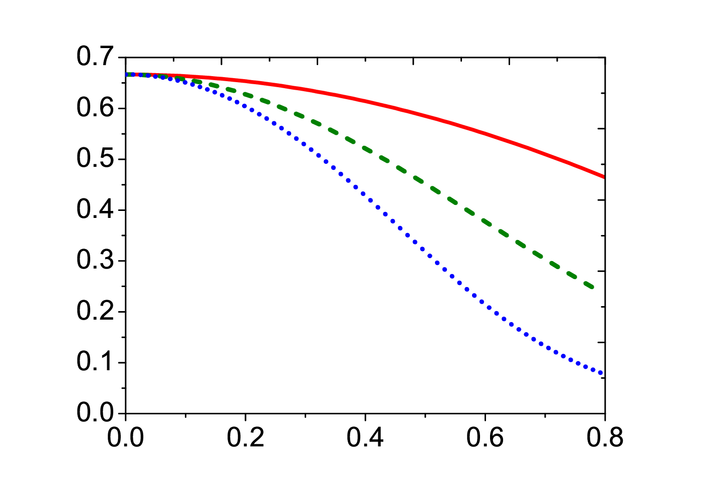
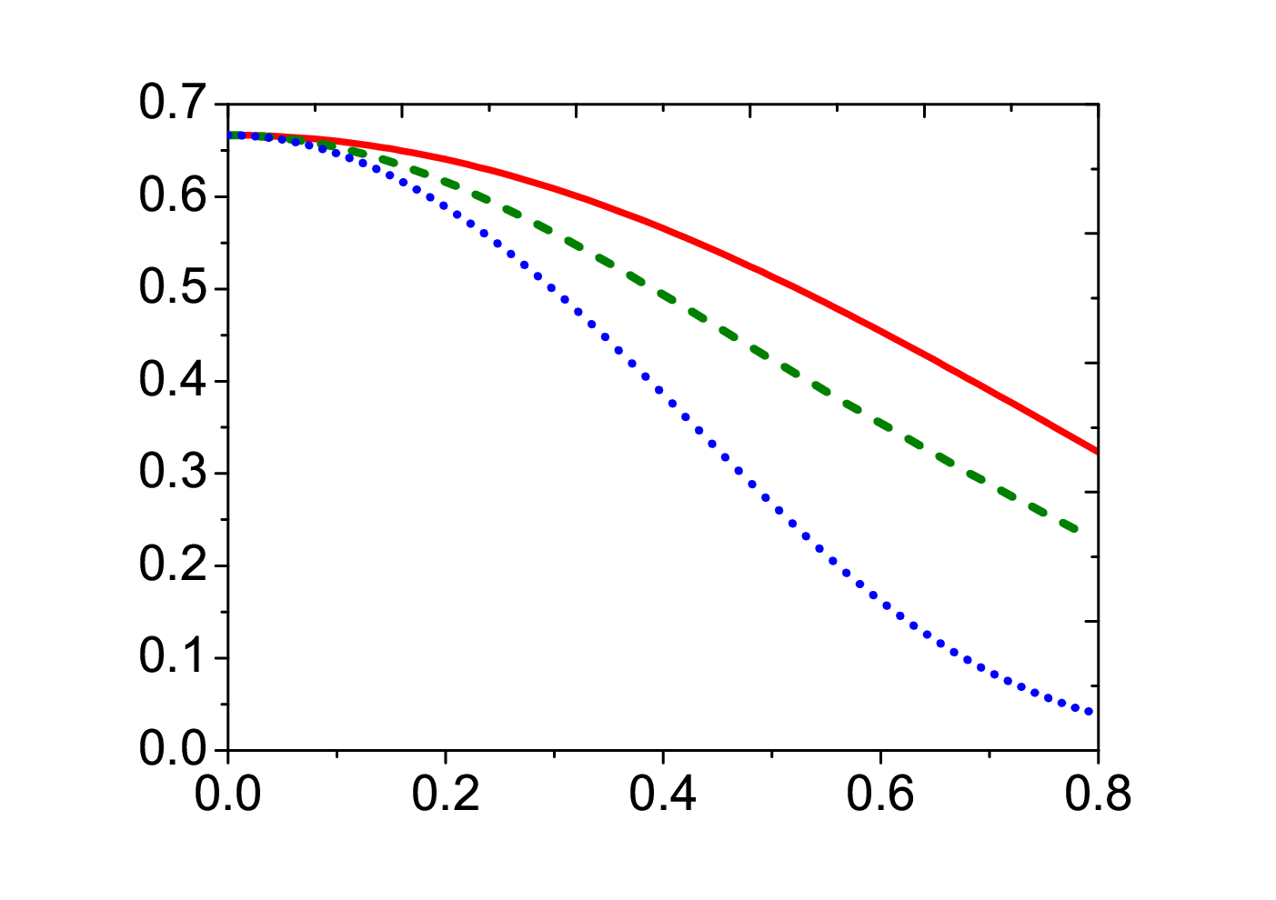
Figure 1: The degree of entanglement ℰ\mathcal{E}, where we assume that rq=rt=rr_{q}=r_{t}=r and (a) s3=1s_{3}=1, t3=1t_{3}=1, and (b)s3=t3=0s_{3}=t_{3}=0. The solid and the dot lines shows the behavior of entanglement when only the qubit and only the qutrit are accelerated respectively.

Finally, let us assume that both particles are accelerated. In this case, the elements of the final state in the first region I1I_{1} are given by,

ρ00,00(q​t)\displaystyle\rho^{(qt)}_{00,00} =\displaystyle= ct4​cq2​ϱ00,00,ρ0​𝒟,0​𝒟(q​t)=cq2​ct2​(ϱ01,01+st2),ρ10,01(q​t)=cq​ct3​(ϱ10,01+ϱ02,01),\displaystyle c_{t}^{4}c^{2}_{q}\varrho_{00,00},\quad\rho^{(qt)}_{0\mathcal{D},0\mathcal{D}}=c^{2}_{q}c^{2}_{t}(\varrho_{01,01}+s_{t}^{2}),\quad\rho^{(qt)}_{10,01}=c_{q}c_{t}^{3}(\varrho_{10,01}+\varrho_{02,01}),
ρ0​𝒰,0​𝒰(q​t)\displaystyle\rho^{(qt)}_{0\mathcal{U},0\mathcal{U}} =\displaystyle= cq2​ct2​(ϱ02,02+ϱ00,00​st2),ρ1​𝒫,0​𝒰(q​t)=−cq​ct​st2​ϱ11,00,\displaystyle c^{2}_{q}c^{2}_{t}(\varrho_{02,02}+\varrho_{00,00}s^{2}_{t}),\quad\rho^{(qt)}_{1\mathcal{P},0\mathcal{U}}=-c_{q}c_{t}s^{2}_{t}\varrho_{11,00},\quad
ρ0​𝒫,0​𝒫(q​t)\displaystyle\rho^{(qt)}_{0\mathcal{P},0\mathcal{P}} =\displaystyle= cq2​st2​(sq2​ϱ00,00+ϱ01,01+ϱ02,02),ρ1​𝒰,0​𝒫(q​t)=−cq​ct​st2​ϱ10,01,ρ01,10=cq​ct3​ϱ01,10,\displaystyle c^{2}_{q}s^{2}_{t}(s^{2}_{q}\varrho_{00,00}+\varrho_{01,01}+\varrho_{02,02}),\quad\rho^{(qt)}_{1\mathcal{U},0\mathcal{P}}=-c_{q}c_{t}s^{2}_{t}\varrho_{10,01},\quad\rho_{01,10}=c_{q}c^{3}_{t}\varrho_{01,10},
ρ10,10(q​t)\displaystyle\rho^{(qt)}_{10,10} =\displaystyle= ct4​(sq2​ϱ00,00+ct4​ϱ10,10),ρ00,1​𝒟(q​t)=cq​ct3​ϱ00,11,\displaystyle c^{4}_{t}(s^{2}_{q}\varrho_{00,00}+c^{4}_{t}\varrho_{10,10}),\quad\rho^{(qt)}_{00,1\mathcal{D}}=c_{q}c^{3}_{t}\varrho_{00,11},
ρ1​𝒟,1​𝒟(q​t)\displaystyle\rho^{(qt)}_{1\mathcal{D},1\mathcal{D}} =\displaystyle= sq2​ct2​(sq2+ϱ01,01)+ct2​(ϱ11,11+st2​ϱ10,10),ρ0​𝒫,1​𝒰(q​t)=−cq​ct​st2​ϱ01,10,\displaystyle s^{2}_{q}c^{2}_{t}(s^{2}_{q}+\varrho_{01,01})+c^{2}_{t}(\varrho_{11,11}+s^{2}_{t}\varrho_{10,10}),\quad\rho^{(qt)}_{0\mathcal{P},1\mathcal{U}}=-c_{q}c_{t}s^{2}_{t}\varrho_{01,10},\quad
ρ1​𝒰,1​𝒰(q​t)\displaystyle\rho^{(qt)}_{1\mathcal{U},1\mathcal{U}} =\displaystyle= sq2​ct2​(ϱ02,02+st2​ϱ00,00)+ct2​(ϱ12,12+st2​ϱ10,10),ρ0​𝒰,1​𝒫(q​t)=−cq​ct​st2​ϱ00,11,\displaystyle s^{2}_{q}c^{2}_{t}(\varrho_{02,02}+s^{2}_{t}\varrho_{00,00})+c^{2}_{t}(\varrho_{12,12}+s^{2}_{t}\varrho_{10,10}),\quad\rho^{(qt)}_{0\mathcal{U},1\mathcal{P}}=-c_{q}c_{t}s^{2}_{t}\varrho_{00,11},\quad
ρ1​𝒫,1​𝒫(q​t)\displaystyle\rho^{(qt)}_{1\mathcal{P},1\mathcal{P}} =\displaystyle= sq2​st2​(ϱ00,00​s2+ϱ01,01+ϱ02,02)+st2​(st2​ϱ10,10+ϱ11,11+ϱ11,01),\displaystyle s^{2}_{q}s^{2}_{t}(\varrho_{00,00}s^{2}+\varrho_{01,01}+\varrho_{02,02})+s^{2}_{t}(s^{2}_{t}\varrho_{10,10}+\varrho_{11,11}+\varrho_{11,01}), (16)

where the suffix "​q​""q", "​t​""t" and "​q​t​""qt" refer to the accelerated qubit, qutrit and qubit-qutrit, respectively.

The behavior of entanglement, ℰ\mathcal{E} is described in Fig.(1a), where we assume that both subsystems are initially polarized on the third direction, namely we set s3=t3=1s_{3}=t_{3}=1. It is clear that, the entanglement decreases as the acceleration of the accelerated subsystems increase. The decay rate of entanglement depends on the accelerated system. However, if the smaller dimensional system is accelerated, then the decay rate of entanglement is smaller than the decay which is caused by accelerating the larger dimensional system. These results are clearly seen by comparing the behavior of endamagement when only the qubit is accelerated (solid-curve)and its behavior when only the qutrit is accelerated (dash-curve). Moreover, the decay rate of entanglement is larger if both subsystems are accelerated.

In Fig.(1b), we consider another system , where we set s2=t3=0s_{2}=t_{3}=0. The general behavior is similar to that shown in Fig.(1a), namely, the entanglement decreases as the accelerations of the subsystem increase. However, the decay rate of entanglement is larger than that depicted in Fig.(1a). This shows that, the entanglement of the initial system plays an essential roles on the degree of entanglement of the accelerated systems.

3.2 One-Parameter Family

This class of qubit-qutrit system is known by one parameter family. The density operator of this system is given by,

ρq​t(1)\displaystyle\rho_{qt}^{(1)} =\displaystyle= |0⟩q​⟨0|{p2​(|0⟩t​⟨0|+|1⟩t​⟨1|)+1−2​p2​|2⟩t​⟨2|}+|1⟩q​⟨0|​{p2​|2⟩t​⟨0|}\displaystyle\bigl|0\bigr\rangle_{q}\bigl\langle 0\bigr|\Bigl\{\frac{p}{2}\left(\bigl|0\bigr\rangle_{t}\bigl\langle 0\bigr|+\bigl|1\bigr\rangle_{t}\bigl\langle 1\bigr|\right)+\frac{1-2p}{2}\bigl|2\bigr\rangle_{t}\bigl\langle 2\bigr|\Bigr\}+\bigl|1\bigr\rangle_{q}\bigl\langle 0\bigr|\Bigl\{\frac{p}{2}\bigl|2\bigr\rangle_{t}\bigl\langle 0\bigr|\Bigr\} (17)
+\displaystyle+ |0⟩q​⟨1​|{p2​|0⟩t​⟨2|+1−2​p2|2⟩t​⟨0|}+|​1⟩q​⟨1|​{p2​|1⟩t​⟨1|+1−2​p2|0⟩t​⟨0|},\displaystyle\bigl|0\bigr\rangle_{q}\bigl\langle 1\bigr|\Bigl\{\frac{p}{2}\bigl|0\bigr\rangle_{t}\bigl\langle 2\bigr|+\frac{1-2p}{2}\bigl|2\bigr\rangle_{t}\bigl\langle 0\bigr|\Bigr\}+\bigl|1\bigr\rangle_{q}\bigl\langle 1\bigr|\Bigl\{\frac{p}{2}\bigl|1\bigr\rangle_{t}\bigl\langle 1\bigr|+\frac{1-2p}{2}\bigl|0\bigr\rangle_{t}\bigl\langle 0\bigr|\Bigr\},

where 0≤p≤120\leq p\leq\frac{1}{2} and the subscript "​q​""q" refers to the qubit while "​t​""t" refers to the qutrit. If we assume that, only the qubit is accelerated, then the density operator of the final state in the first region (I)(I) is defined by the following non-zero elements, of a matrix of size 2×32\times 3,

ρ00,00(1q)\displaystyle\rho^{(1_{q})}_{00,00} =\displaystyle= p2​cq2,ρ00,12(1q)=p2​cq,ρ01,01(1q)=p2​cq2,ρ00,12(1q)=ρ12,00,\displaystyle\frac{p}{2}c^{2}_{q},\quad\rho^{(1_{q})}_{00,12}=\frac{p}{2}c_{q},\quad\rho^{(1_{q})}_{01,01}=\frac{p}{2}c^{2}_{q},\quad\rho^{(1_{q})}_{00,12}=\rho_{12,00},
ρ02,02(1q)\displaystyle\rho^{(1_{q})}_{02,02} =\displaystyle= 1−2​p2​cq2,ρ10,02(1q)=1−2​p2​cq,ρ10,10(1q)=(1−2​p2+p2​sq2),\displaystyle\frac{1-2p}{2}c^{2}_{q},\quad\rho^{(1_{q})}_{10,02}=\frac{1-2p}{2}c_{q},\quad\rho^{(1_{q})}_{10,10}=\left(\frac{1-2p}{2}+\frac{p}{2}s^{2}_{q}\right),
ρ02,10(1q)\displaystyle\rho^{(1_{q})}_{02,10} =\displaystyle= ρ10,02,ρ11,11(1q)=p2​(1+sq2),ρ12,12(1q)=(1−2​p2​sq2+p2).\displaystyle\rho_{10,02},\quad\rho^{(1_{q})}_{11,11}=\frac{p}{2}(1+s^{2}_{q}),\quad\rho^{(1_{q})}_{12,12}=\left(\frac{1-2p}{2}s^{2}_{q}+\frac{p}{2}\right).\quad (18)

On the other hand, if only the qutrit is accelerated, then the final state of the total system in the first region is defined by a matrix of size 8×88\times 8. The non-zero elements are given by,

Refer to caption

r E

Figure 2: The entanglement of one parameter family evaluated at p=0.5,rq=rt=rp=0.5,r_{q}=r_{t}=r. The solid, dash and dot curves represent the entanglement ℰ\mathcal{E}, when only the qubit , only the qutrit, and both of them are accelerated.
ρ00,00(1t)\displaystyle\rho^{(1_{t})}_{00,00} =\displaystyle= p2​ct4,ρ12,00(1t)=p2​ct3,ρ0​𝒟,0​𝒟(1t)=p2​ct2​(1+st2),ρ1​𝒫,0​𝒟(1t)=p2​ct​st2,\displaystyle\frac{p}{2}c^{4}_{t},\quad\rho^{(1_{t})}_{12,00}=\frac{p}{2}c^{3}_{t},\quad\rho^{(1_{t})}_{0\mathcal{D},0\mathcal{D}}=\frac{p}{2}c^{2}_{t}(1+s^{2}_{t}),\quad\rho^{(1_{t})}_{1\mathcal{P},0\mathcal{D}}=\frac{p}{2}c_{t}s^{2}_{t},
ρ0​𝒰,0​𝒰(1t)\displaystyle\rho^{(1_{t})}_{0\mathcal{U},0\mathcal{U}} =\displaystyle= ct2​(1−2​p2+p2​st2),ρ10,02(1t)=1−2​p2​ct3,ρ0​𝒫,0​𝒫(1t)=st2​(p2​(1+st2)+1−2​p2),\displaystyle c^{2}_{t}\left(\frac{1-2p}{2}+\frac{p}{2}s^{2}_{t}\right),\quad\rho^{(1_{t})}_{10,02}=\frac{1-2p}{2}c^{3}_{t},\quad\rho^{(1_{t})}_{0\mathcal{P},0\mathcal{P}}=s^{2}_{t}\left(\frac{p}{2}(1+s_{t}^{2})+\frac{1-2p}{2}\right),
ρ1​𝒟,0​𝒫(1t)\displaystyle\rho^{(1_{t})}_{1\mathcal{D},0\mathcal{P}} =\displaystyle= 1−2​p2​ct​st2,ρ10,10(1t)=1−2​p2​ct4,ρ0​𝒰,10(1t)=ρ10,0​𝒰(1t),ρ1​𝒟,1​𝒟(1t)=1−2​p2​ct2​st2,\displaystyle\frac{1-2p}{2}c_{t}s^{2}_{t},\quad\rho^{(1_{t})}_{10,10}=\frac{1-2p}{2}c^{4}_{t},\quad\rho^{(1_{t})}_{0\mathcal{U},10}=\rho^{(1_{t})}_{10,0\mathcal{U}},\quad\rho^{(1_{t})}_{1\mathcal{D},1\mathcal{D}}=\frac{1-2p}{2}c^{2}_{t}s^{2}_{t},\quad
ρ0​𝒫,1​𝒟(1t)\displaystyle\rho^{(1_{t})}_{0\mathcal{P},1\mathcal{D}} =\displaystyle= 1−2​p2​ct​st2,ρ00,1​𝒰(1t)=ρ12,00(1t),ρ1​𝒰,1​𝒰(1t)=ct2​(p2+1−2​pp​st2),\displaystyle\frac{1-2p}{2}c_{t}s^{2}_{t},\quad\rho^{(1_{t})}_{00,1\mathcal{U}}=\rho^{(1_{t})}_{12,00},\quad\rho^{(1_{t})}_{1\mathcal{U},1\mathcal{U}}=c^{2}_{t}\left(\frac{p}{2}+\frac{1-2p}{p}s^{2}_{t}\right),
ρ0​𝒟,1​𝒫(1t)\displaystyle\rho^{(1_{t})}_{0\mathcal{D},1\mathcal{P}} =\displaystyle= p2​ct​st2,ρ1​𝒫,1​𝒫(1t)=st2​(p+1−2​p2​st2).\displaystyle\frac{p}{2}c_{t}s^{2}_{t},\quad\rho^{(1_{t})}_{1\mathcal{P},1\mathcal{P}}=s^{2}_{t}\left(p+\frac{1-2p}{2}s_{t}^{2}\right). (19)

Finally, if both subsystems are accelerated, then the final state in the first region, II is defined by the following non-zero elements of a matrix of 8×88\times 8,

ρ00,00(1q​t)\displaystyle\rho^{(1_{qt})}_{00,00} =\displaystyle= cq2​ρ00,00(1t),ρ1​𝒟,00(1q​t)=p2​cq​ct3,ρ0​𝒟,0​𝒟(1q​t)=cq2​ρ0​𝒟,0​𝒟(1t),ρ1​𝒫,0​𝒟(1q​t)=cq​ρ1​𝒫,0​𝒟(1t),\displaystyle c^{2}_{q}\rho^{(1_{t})}_{00,00},\quad\rho^{(1_{qt})}_{1\mathcal{D},00}=\frac{p}{2}c_{q}c^{3}_{t},\quad\rho^{(1_{qt})}_{0\mathcal{D},0\mathcal{D}}=c^{2}_{q}\rho^{(1_{t})}_{0\mathcal{D},0\mathcal{D}},\quad\rho^{(1_{qt})}_{1\mathcal{P},0\mathcal{D}}=c_{q}\rho^{(1_{t})}_{1\mathcal{P},0\mathcal{D}},
ρ0​𝒰,0​𝒰(1q​t)\displaystyle\rho^{(1_{qt})}_{0\mathcal{U},0\mathcal{U}} =\displaystyle= cq2​ρ0​𝒰,0​𝒰(1t),ρ10,0​𝒰(1q​t)=cq​ρ10,0​𝒰(1t),ρ0​𝒫,0​𝒫(1q​t)=cq2​ρ0​𝒫,0​𝒫(1t),ρ1​𝒟,0​𝒫(1q​t)=cq​ρ1​𝒟,0​𝒫(1t),\displaystyle c^{2}_{q}\rho^{(1_{t})}_{0\mathcal{U},0\mathcal{U}},\quad\rho^{(1_{qt})}_{10,0\mathcal{U}}=c_{q}\rho^{(1_{t})}_{10,0\mathcal{U}},\quad\rho^{(1_{qt})}_{0\mathcal{P},0\mathcal{P}}=c^{2}_{q}\rho^{(1_{t})}_{0\mathcal{P},0\mathcal{P}},\quad\rho^{(1_{qt})}_{1\mathcal{D},0\mathcal{P}}=c_{q}\rho^{(1_{t})}_{1\mathcal{D},0\mathcal{P}},
ρ10,10(1q​t)\displaystyle\rho^{(1_{qt})}_{10,10} =\displaystyle= ρ10,10(1t)+p2​ct4​sq2,ρ0​𝒟,10(1q​t)=cq​ρ10,0​𝒰(1t),ρ1​𝒟,1​𝒟(1q​t)=ρ1​𝒟,1​𝒟(1t)+ct2​p2​(1+sq2+sq2​st2),\displaystyle\rho^{(1_{t})}_{10,10}+\frac{p}{2}c^{4}_{t}s^{2}_{q},\quad\rho^{(1_{qt})}_{0\mathcal{D},10}=c_{q}\rho^{(1_{t})}_{10,0\mathcal{U}},\quad\rho^{(1_{qt})}_{1\mathcal{D},1\mathcal{D}}=\rho^{(1_{t})}_{1\mathcal{D},1\mathcal{D}}+c^{2}_{t}\frac{p}{2}\left(1+s^{2}_{q}+s^{2}_{q}s^{2}_{t}\right),
ρ0​𝒫,1​𝒟(1q​t)\displaystyle\rho^{(1_{qt})}_{0\mathcal{P},1\mathcal{D}} =\displaystyle= cq​ρ0​𝒫,1​𝒟(1t),ρ1​𝒰,1​𝒰(1q​t)=ρ1​𝒰,1​𝒰(1t)+ct2​(p2​(1+st2​sq2)+1−2​p2​sq2),ρ00,1​𝒰(1q​t)=cq​ρ00,1​𝒰(1t),\displaystyle c_{q}\rho^{(1_{t})}_{0\mathcal{P},1\mathcal{D}},\quad\rho^{(1_{qt})}_{1\mathcal{U},1\mathcal{U}}=\rho^{(1_{t})}_{1\mathcal{U},1\mathcal{U}}+c^{2}_{t}\left(\frac{p}{2}(1+s^{2}_{t}s^{2}_{q})+\frac{1-2p}{2}s^{2}_{q}\right),\quad\rho^{(1_{qt})}_{00,1\mathcal{U}}=c_{q}\rho^{(1_{t})}_{00,1\mathcal{U}},
ρ1​𝒫,1​𝒫(1q​t)\displaystyle\rho^{(1_{qt})}_{1\mathcal{P},1\mathcal{P}} =\displaystyle= ρ1​𝒫,1​𝒫(1t)+sq2​st2​(p2​st2+1−p2),ρ01,1​𝒫(1q​t)=cq​ρ0​𝒟,1​𝒫(1t).\displaystyle\rho^{(1_{t})}_{1\mathcal{P},1\mathcal{P}}+s^{2}_{q}s^{2}_{t}\left(\frac{p}{2}s^{2}_{t}+\frac{1-p}{2}\right),\quad\rho^{(1_{qt})}_{01,1\mathcal{P}}=c_{q}\rho^{(1_{t})}_{0\mathcal{D},1\mathcal{P}}. (20)

The behavior of entanglement for this case is shown in Fig.(2), where we initially start with a system defined by p=0.5p=0.5. The general behavior is similar to that shown in Fig.(1), namely the entanglement decays as the the acceleration of the accelerated subsystem increases. The upper and lower bounds of entanglement depend on the accelerated subsystem and the initial degree of entanglement. However, if the qubit is allowed to be accelerated, then the upper bounds of entanglement are always larger than that shown if one allows the qutrit to be accelerated. The decay rate of entanglement increases if both particles are accelerated, where we considered both particles are accelerated with the same acceleration (i.e., rq=rt=rr_{q}=r_{t}=r).

3.3 Two-Parameters family

In this subsection we consider the second example which is known by a two-parameter family. In the computational basis, this class can be written as,

ρq​t(2)\displaystyle\rho^{(2)}_{qt} =\displaystyle= |0⟩q​⟨0​|{β​|0⟩t​⟨0|+β+γ2|1⟩t​⟨1|+α|2⟩t​⟨2|}+|​1⟩q​⟨0|​{β−γ2​|0⟩t​⟨1|}\displaystyle\bigl|0\bigr\rangle_{q}\bigl\langle 0\bigr|\Bigl\{\beta\bigl|0\bigr\rangle_{t}\bigl\langle 0\bigr|+\frac{\beta+\gamma}{2}\bigl|1\bigr\rangle_{t}\bigl\langle 1\bigr|+\alpha\bigl|2\bigr\rangle_{t}\bigl\langle 2\bigr|\Bigr\}+\bigl|1\bigr\rangle_{q}\bigl\langle 0\bigr|\Bigl\{\frac{\beta-\gamma}{2}\bigl|0\bigr\rangle_{t}\bigl\langle 1\bigr|\Bigr\} (21)
+|0⟩q​⟨1|{β−γ2​|1⟩t​⟨0|}+|1⟩q​⟨1|​{β+γ2​|0⟩t​⟨0|+β|1⟩​⟨1|+α|2⟩t​⟨2|},\displaystyle+\bigl|0\bigr\rangle_{q}\bigl\langle 1\bigr|\Bigl\{\frac{\beta-\gamma}{2}\bigl|1\bigr\rangle_{t}\bigl\langle 0\bigr|\Bigr\}+\bigl|1\bigr\rangle_{q}\bigl\langle 1\bigr|\Bigl\{\frac{\beta+\gamma}{2}\bigl|0\bigr\rangle_{t}\bigl\langle 0\bigr|+\beta\bigl|1\bigr\rangle\bigl\langle 1\bigr|+\alpha\bigl|2\bigr\rangle_{t}\bigl\langle 2\bigr|\Bigr\},\quad

where γ+2​α+3​β=1\gamma+2\alpha+3\beta=1 and the suffix 22 refers to the two-parameter. If it assumed that only the qubit is accelerated, then the final state in the first region, II of the Rindler space is described by the following non-zero-elements of a matrix of size 6×66\times 6,

ρ00,00(2q)\displaystyle\rho^{(2_{q})}_{00,00} =\displaystyle= β​cq2,ρ01,01(2q)=β+γ2​cq2,ρ10,01(2q)=β−γ2​cq,\displaystyle\beta c^{2}_{q},\quad\rho^{(2_{q})}_{01,01}=\frac{\beta+\gamma}{2}c^{2}_{q},\quad\rho^{(2_{q})}_{10,01}=\frac{\beta-\gamma}{2}c_{q},
ρ02,02(2q)\displaystyle\rho^{(2_{q})}_{02,02} =\displaystyle= α​cq2,ρ01,10(2q)=β−γ2​cq,ρ10,10=β​sq2,\displaystyle\alpha c^{2}_{q},\quad\rho^{(2_{q})}_{01,10}=\frac{\beta-\gamma}{2}c_{q},\quad\rho_{10,10}=\beta s^{2}_{q},
ρ11,11(2q)\displaystyle\rho^{(2_{q})}_{11,11} =\displaystyle= (β+β+γ2​sq2),ρ12,12(2q)=α⁡(1+sq2).\displaystyle\left(\beta+\frac{\beta+\gamma}{2}s^{2}_{q}\right),\quad\rho^{(2_{q})}_{12,12}=\alpha(1+s^{2}_{q}). (22)

On the other hand, if we consider only the qutrit is accelerated then, the final state in the first Rindler region is defined by the following non-zero elements,

ρ00,00(2t)\displaystyle\rho^{(2_{t})}_{00,00} =\displaystyle= β​ct4,ρ01,0​𝒟(2t)=ct2​(β​st2+β+γ2),ρ10,0​𝒟(2t)=β−γ2​ct3,\displaystyle\beta c^{4}_{t},\quad\rho^{(2_{t})}_{01,0\mathcal{D}}=c^{2}_{t}\left(\beta s^{2}_{t}+\frac{\beta+\gamma}{2}\right),\quad\rho^{(2_{t})}_{10,0\mathcal{D}}=\frac{\beta-\gamma}{2}c^{3}_{t},
ρ0​𝒰,0​𝒰(2t)\displaystyle\rho^{(2_{t})}_{0\mathcal{U},0\mathcal{U}} =\displaystyle= ct2(α+βst2),ρ0​𝒫,0​𝒫(2t)=st2((α+3​β+γ2st2),ρ1​𝒰,0​𝒫(2t)=−β−γ2ctst2,\displaystyle c^{2}_{t}(\alpha+\beta s^{2}_{t}),\quad\rho^{(2_{t})}_{0\mathcal{P},0\mathcal{P}}=s^{2}_{t}(\left(\alpha+\frac{3\beta+\gamma}{2}s^{2}_{t}\right),\quad\rho^{(2_{t})}_{1\mathcal{U},0\mathcal{P}}=-\frac{\beta-\gamma}{2}c_{t}s^{2}_{t},
ρ0​𝒟,10(2t)\displaystyle\rho^{(2_{t})}_{0\mathcal{D},10} =\displaystyle= β−γ2​ct3,ρ10,10(2t)=β+γ2​ct4,ρ1​𝒟,1​𝒟(2t)=ct2​(β+β+γ2​st2),ρ0​𝒫,1​𝒰(2t)=ρ1​𝒰,0​𝒫(2t)\displaystyle\frac{\beta-\gamma}{2}c^{3}_{t},\quad\rho^{(2_{t})}_{10,10}=\frac{\beta+\gamma}{2}c^{4}_{t},\quad\rho^{(2_{t})}_{1\mathcal{D},1\mathcal{D}}=c^{2}_{t}\left(\beta+\frac{\beta+\gamma}{2}s^{2}_{t}\right),\quad\rho^{(2_{t})}_{0\mathcal{P},1\mathcal{U}}=\rho^{(2_{t})}_{1\mathcal{U},0\mathcal{P}}
ρ1​𝒰,1​𝒰(2t)\displaystyle\rho^{(2_{t})}_{1\mathcal{U},1\mathcal{U}} =\displaystyle= ct2​(α+β+γ2​st2),ρ1​𝒫,1​𝒫(2t)=st2​(α+3​β+γ2​st2).\displaystyle c^{2}_{t}\left(\alpha+\frac{\beta+\gamma}{2}s^{2}_{t}\right),\quad\rho^{(2_{t})}_{1\mathcal{P},1\mathcal{P}}=s^{2}_{t}\left(\alpha+\frac{3\beta+\gamma}{2}s^{2}_{t}\right). (23)

Finally, when both subsystems are accelerated, then the final state in the first region, II is defined by a matrix of size 8×88\times 8 elements. These elements can be written by (22) as,

ρ00,00(2q​t)\displaystyle\rho_{00,00}^{(2_{qt})} =\displaystyle= cq2​ρ00,00(2t),ρ0​𝒟,0​𝒟(2q​t)=cq2​ρ0​𝒟,0​𝒟(2t),ρ10,0​𝒟(2q​t)=cq​ρ10,0​𝒟(2t),ρ0​𝒰,0​𝒰(2q​t)=cq2​ρ0​𝒰,0​𝒰(2t)\displaystyle c^{2}_{q}\rho^{(2_{t})}_{00,00},\quad\rho^{(2_{qt})}_{0\mathcal{D},0\mathcal{D}}=c^{2}_{q}\rho^{(2_{t})}_{0\mathcal{D},0\mathcal{D}},\quad\rho^{(2_{qt})}_{10,0\mathcal{D}}=c_{q}\rho^{(2_{t})}_{10,0\mathcal{D}},\quad\rho^{(2_{qt})}_{0\mathcal{U},0\mathcal{U}}=c^{2}_{q}\rho^{(2_{t})}_{0\mathcal{U},0\mathcal{U}}
ρ0​𝒫,0​𝒫(2q​t)\displaystyle\rho^{(2_{qt})}_{0\mathcal{P},0\mathcal{P}} =\displaystyle= cq2​ρ0​𝒫,0​𝒫(2t),ρ1​𝒰,0​𝒫(2q​t)=cq​ρ1​𝒰,0​𝒫(2t),ρ0​𝒟​10(2q​t)=cq​ρ0​𝒟,10(2t),ρ10,10(2q​t)=sq2​ρ10,10(2t),\displaystyle c^{2}_{q}\rho^{(2_{t})}_{0\mathcal{P},0\mathcal{P}},\quad\rho^{(2_{qt})}_{1\mathcal{U},0\mathcal{P}}=c_{q}\rho^{(2_{t})}_{1\mathcal{U},0\mathcal{P}},\quad\rho^{(2_{qt})}_{0\mathcal{D}10}=c_{q}\rho^{(2_{t})}_{0\mathcal{D},10},\quad\rho^{(2_{qt})}_{10,10}=s^{2}_{q}\rho^{(2_{t})}_{10,10},
ρ1​𝒟,1​𝒟(2q​t)\displaystyle\rho^{(2_{qt})}_{1\mathcal{D},1\mathcal{D}} =\displaystyle= ρ11,11(2t)+sq2​ρ0​𝒟,0​𝒟(2t),ρ0​𝒫,1​𝒰(2q​t)=ρ1​𝒰,0​𝒫(2q​t),ρ1​𝒰,1​𝒰(2q​t)=ρ1​𝒰,1​𝒰(2t)+sq2​ρ0​𝒰,0​𝒰(2t),\displaystyle\rho^{(2_{t})}_{11,11}+s^{2}_{q}\rho^{(2_{t})}_{0\mathcal{D},0\mathcal{D}},\quad\rho^{(2_{qt})}_{0\mathcal{P},1\mathcal{U}}=\rho^{(2_{qt})}_{1\mathcal{U},0\mathcal{P}},\quad\rho^{(2_{qt})}_{1\mathcal{U},1\mathcal{U}}=\rho^{(2_{t})}_{1\mathcal{U},1\mathcal{U}}+s^{2}_{q}\rho^{(2_{t})}_{0\mathcal{U},0\mathcal{U}},
ρ1​p,1​p(2q​t)\displaystyle\rho^{(2_{qt})}_{1p,1p} =\displaystyle= ρ1​𝒫,1​𝒫(2t)+sq2​ρ0​𝒫,0​𝒫(2t),\displaystyle\rho^{(2_{t})}_{1\mathcal{P},1\mathcal{P}}+s^{2}_{q}\rho^{(2_{t})}_{0\mathcal{P},0\mathcal{P}}, (24)
Refer to caption

r E

Figure 3: The dynamics of entanglement in the first region for qubit-qutrit system of two-parameter family with α=β=0.5\alpha=\beta=0.5. The solid, dash and dot-curves represent ℰ\mathcal{E}, when only the qubit, qutrit and both qubit and qutrit are accelerated.

The behavior of entanglement for this class is described in Fig.(3), where all the three possibilities are considered. It is assumed that, the system is initially prepared in maximum entangled state α=β=0.5\alpha=\beta=0.5. Therefore the entanglement is maximum i.e., ℰ=1\mathcal{E}=1 at rq=rt=0r_{q}=r_{t}=0. It is clear that, the behavior of entanglement is similar to that predicated for one parameter family. However, the entanglement decays as the acceleration of any subsystem increases, where we consider that, both of the subsystems have the same acceleration (rq=rt)(r_{q}=r_{t}). The rate of entanglement decay increases as the dimensions of the accelerated subsystems increase. Moreover, if both subsystems are accelerated, then the entanglement decreases faster.

4 Conclusion

In this contribution, we consider a general system composite of two different dimensions. One of them is a two-dimensional qubit and the other is of three dimensional qutrit. It is assumed that, one or both subsystems are accelerated simultaneously or non- simultaneously. The density operator of the final state in the first region of the accelerated is obtained analytical in a general form. Different examples are introduced to show the main task of this manuscript.

Our results show that, the entanglement decays as the acceleration of the accelerated particle increases. However, the decay rate depends on the dimensions of the accelerated subsystem. If only the qubit is accelerated, then the entanglement decays gradually to reach its non-zero values at infinity. On the other hand, if we allow only the qutrit to be accelerated, then the entanglement decays faster and its upper bounds always smaller than that depicted for accelerating qubit. Moreover, if one allows for both subsystems to be accelerated, then the decay rate of entanglement is larger.

The idea is shown explicitly by considering three different and common examples. In the first example, we assume that both subsystems are polarized in z−z-axis. It is clear that, the decay of entanglement depends on the initial correlation between the two subsystems. The second and third examples are known by one and two-parameters families. These examples have been investigated widely in the context of quantum information. It is shown that the decay rate of entanglement depends on the initial degree of entanglement in addition to the dimensions of the accelerated subsystem.

In conclusion: the decay of entanglement depends on the dimensions of the accelerated subsystems, where the decay rate of entanglement increases when the larger dimensional subsystem is accelerated. The robustness of the accelerated system depends on the initial quantum correlation between the two subsystems. We expect that these results could be important in building an accelerated quantum network consists of different dimensions nodes.

Appendices

Appendix A The elements of the initial state

The elements of the initial system (1) in the basis |00⟩,|01⟩,|02⟩,|10⟩,|11⟩\bigl|00\bigr\rangle,\bigl|01\bigr\rangle,\bigl|02\bigr\rangle,\bigl|10\bigr\rangle,\bigl|11\bigr\rangle and |12⟩\bigl|12\bigr\rangle are given by.

𝒜1\displaystyle\mathcal{A}_{1} =\displaystyle= (1+s3+t3−c33+t8/3−c38/3)/6,𝒜2=(t1−i​t2−c31+i​c32)/6,\displaystyle(1+s_{3}+t_{3}-c_{33}+t_{8}/\sqrt{3}-c_{38}/\sqrt{3})/6,\quad\mathcal{A}_{2}=(t_{1}-it_{2}-c_{31}+ic_{32})/6,
𝒜3\displaystyle\mathcal{A}_{3} =\displaystyle= (t4−i​t5−c34+i​c35)/6,𝒜4=(s1+i​s2+c13+i​c23+c18/3+i​c28/3)/6,\displaystyle(t_{4}-it_{5}-c_{34}+ic_{35})/6,\quad\mathcal{A}_{4}=(s_{1}+is_{2}+c_{13}+ic_{23}+c_{18}/\sqrt{3}+ic_{28}/\sqrt{3})/6,
𝒜5\displaystyle\mathcal{A}_{5} =\displaystyle= (c11−c22+i​c21−i​c12)/6,𝒜6=(c14+c25+i​c24−i​c15)/6,\displaystyle(c_{11}-c_{22}+ic_{21}-ic_{12})/6,\quad\mathcal{A}_{6}=(c_{14}+c_{25}+ic_{24}-ic_{15})/6,
𝒜7\displaystyle\mathcal{A}_{7} =\displaystyle= (t1+i​t2−c31−i​c32)/6,𝒜8=(1−s3−t3+t8/3+c33−c38/3)/6,\displaystyle(t_{1}+it_{2}-c_{31}-ic_{32})/6,\quad\mathcal{A}_{8}=(1-s_{3}-t_{3}+t_{8}/\sqrt{3}+c_{33}-c_{38}/\sqrt{3})/6,
𝒜9\displaystyle\mathcal{A}_{9} =\displaystyle= (t6−i​t7−c36+i​c37)/6,𝒜10=(c11−c22+i​c12−i​c21)/6,\displaystyle(t_{6}-it_{7}-c_{36}+ic_{37})/6,\quad\mathcal{A}_{10}=(c_{11}-c_{22}+ic_{12}-ic_{21})/6,
𝒜11\displaystyle\mathcal{A}_{11} =\displaystyle= (s1+i​s2−c13+−i​c23+c18/3+i​c28/3)/6,𝒜12=(c16+c27+i​c26−i​c17)/6,\displaystyle(s_{1}+is_{2}-c_{13}+-ic_{23}+c_{18}/\sqrt{3}+ic_{28}/\sqrt{3})/6,\quad\mathcal{A}_{12}=(c_{16}+c_{27}+ic_{26}-ic_{17})/6,
𝒜13\displaystyle\mathcal{A}_{13} =\displaystyle= (t4+i​t5−c34−i​c35)/6,𝒜14=(t6+i​t7−c36−i​c37)/6,\displaystyle(t_{4}+it_{5}-c_{34}-ic_{35})/6,\quad\mathcal{A}_{14}=(t_{6}+it_{7}-c_{36}-ic_{37})/6,
𝒜15\displaystyle\mathcal{A}_{15} =\displaystyle= (1−s3−2​t8/3+2​c38/3)/6,𝒜16=(c14−c25+i​c15+i​c24)/6,\displaystyle(1-s_{3}-2t_{8}/\sqrt{3}+2c_{38}/\sqrt{3})/6,\quad\mathcal{A}_{16}=(c_{14}-c_{25}+ic_{15}+ic_{24})/6,
𝒜17\displaystyle\mathcal{A}_{17} =\displaystyle= (c16−c27+i​c17+i​c26)/6,𝒜18=(s1+i​s2−2​c28/3−2​c18/3)/6,\displaystyle(c_{16}-c_{27}+ic_{17}+ic_{26})/6,\quad\mathcal{A}_{18}=(s_{1}+is_{2}-2c_{28}/\sqrt{3}-2c_{18}/\sqrt{3})/6,
𝒜19\displaystyle\mathcal{A}_{19} =\displaystyle= (s1+i​s2+c13−i​c23+c18/3−i​c28/3)/6,𝒜20=(c11−c22−i​c12−i​c21)/6,\displaystyle(s_{1}+is_{2}+c_{13}-ic_{23}+c_{18}/\sqrt{3}-ic_{28}/\sqrt{3})/6,\quad\mathcal{A}_{20}=(c_{11}-c_{22}-ic_{12}-ic_{21})/6,\quad
𝒜21\displaystyle\mathcal{A}_{21} =\displaystyle= (c14−c25−i​c15−i​c24)/6,𝒜22=(1+s3+t3+t8/3+c33+c38/3)/6,\displaystyle(c_{14}-c_{25}-ic_{15}-ic_{24})/6,\quad\mathcal{A}_{22}=(1+s_{3}+t_{3}+t_{8}/\sqrt{3}+c_{33}+c_{38}/\sqrt{3})/6,
𝒜23\displaystyle\mathcal{A}_{23} =\displaystyle= (t1−i​t2+c31−i​c32)/6,𝒜24=(t4−i​t5+c34−i​c35)/6,\displaystyle(t_{1}-it_{2}+c_{31}-ic_{32})/6,\quad\mathcal{A}_{24}=(t_{4}-it_{5}+c_{34}-ic_{35})/6,\quad
𝒜25\displaystyle\mathcal{A}_{25} =\displaystyle= (c11+c22+i​c12−i​c21)/6,𝒜26=(s1−i​s2−c13+i​c23+c18/3−i​c28/3)/6,\displaystyle(c_{11}+c_{22}+ic_{12}-ic_{21})/6,\quad\mathcal{A}_{26}=(s_{1}-is_{2}-c_{13}+ic_{23}+c_{18}/\sqrt{3}-ic_{28}/\sqrt{3})/6,
𝒜27\displaystyle\mathcal{A}_{27} =\displaystyle= (c16−c27−ic17−ic26)/6,𝒜28=−(t1+it2+c31+ic32)/6,\displaystyle(c_{16}-c_{27}-ic_{17}-ic_{26})/6,\quad\mathcal{A}_{28}=-(t_{1}+it_{2}+c_{31}+ic_{32})/6,
𝒜29\displaystyle\mathcal{A}_{29} =\displaystyle= (1+s3−t3+t8/3−c33+c38/3)/6,𝒜30=(t6−i​t7+c36−i​c37)/6,\displaystyle(1+s_{3}-t_{3}+t_{8}/\sqrt{3}-c_{33}+c_{38}/\sqrt{3})/6,\quad\mathcal{A}_{30}=(t_{6}-it_{7}+c_{36}-ic_{37})/6,\quad
𝒜31\displaystyle\mathcal{A}_{31} =\displaystyle= (c14+c25+i​c15+i​c24)/6,𝒜32=(c16+c27+i​c17−i​c26)/6,\displaystyle(c_{14}+c_{25}+ic_{15}+ic_{24})/6,\quad\mathcal{A}_{32}=(c_{16}+c_{27}+ic_{17}-ic_{26})/6,
𝒜33\displaystyle\mathcal{A}_{33} =\displaystyle= (s1−i​s2+2​i​c28/3−2​c18/3)/6,𝒜34=(t6+i​t7+c36+i​c37)/6,\displaystyle(s_{1}-is_{2}+2ic_{28}/\sqrt{3}-2c_{18}/\sqrt{3})/6,\quad\mathcal{A}_{34}=(t_{6}+it_{7}+c_{36}+ic_{37})/6,\quad
𝒜35\displaystyle\mathcal{A}_{35} =\displaystyle= (t4+i​t5+c34+i​c35)/6,𝒜36=(1+s3−2​t8/3−2​c38/3)/6.\displaystyle(t_{4}+it_{5}+c_{34}+ic_{35})/6,\quad\mathcal{A}_{36}=(1+s_{3}-2t_{8}/\sqrt{3}-2c_{38}/\sqrt{3})/6. (25)

Appendix B Both subsystems are accelerated

The parameters ℬi,i,1..52\mathcal{B}_{i},i,1..52 which are appeared in Eq.(11) are give explicitly as,

ℬ1\displaystyle\mathcal{B}_{1} =\displaystyle= cq2​ct4​𝒜1,ℬ2=cq2​𝒜2,ℬ3=cq2​𝒜3+cq​𝒜6,ℬ4=cq​ct4​𝒜4,ℬ5=cq​ct3​𝒜5,\displaystyle c^{2}_{q}c^{4}_{t}\mathcal{A}_{1},\quad\mathcal{B}_{2}=c^{2}_{q}\mathcal{A}_{2},\quad\mathcal{B}_{3}=c^{2}_{q}\mathcal{A}_{3}+c_{q}\mathcal{A}_{6},\quad\mathcal{B}_{4}=c_{q}c^{4}_{t}\mathcal{A}_{4},\quad\mathcal{B}_{5}=c_{q}c^{3}_{t}\mathcal{A}_{5},
ℬ6\displaystyle\mathcal{B}_{6} =\displaystyle= cq2​ct3​𝒜6,ℬ7=cq2​ct2​(𝒜8+st2​𝒜1),ℬ8=cq​ct2​𝒜9,ℬ9=cq2​ct​st2​𝒜3,ℬ10=cq​ct3​𝒜10\displaystyle c^{2}_{q}c^{3}_{t}\mathcal{A}_{6},\quad\mathcal{B}_{7}=c^{2}_{q}c^{2}_{t}(\mathcal{A}_{8}+s^{2}_{t}\mathcal{A}_{1}),\quad\mathcal{B}_{8}=c^{q}c^{2}_{t}\mathcal{A}_{9},\quad\mathcal{B}_{9}=c^{2}_{q}c_{t}s^{2}_{t}\mathcal{A}_{3},\quad\mathcal{B}_{10}=c_{q}c^{3}_{t}\mathcal{A}_{10}
ℬ11\displaystyle\mathcal{B}_{11} =\displaystyle= cq​ct2​(𝒜11+st2​𝒜4),ℬ12=cq​ct2​𝒜12,ℬ13=cq​st2​𝒜6,ℬ14=cq2​ct3​𝒜13,ℬ15=cq2​ct2​𝒜14\displaystyle c_{q}c^{2}_{t}(\mathcal{A}_{11}+s^{2}_{t}\mathcal{A}_{4}),\quad\mathcal{B}_{12}=c_{q}c^{2}_{t}\mathcal{A}_{12},\quad\mathcal{B}_{13}=c_{q}s^{2}_{t}\mathcal{A}_{6},\quad\mathcal{B}_{14}=c^{2}_{q}c^{3}_{t}\mathcal{A}_{13},\quad\mathcal{B}_{15}=c^{2}_{q}c^{2}_{t}\mathcal{A}_{14}
ℬ16\displaystyle\mathcal{B}_{16} =\displaystyle= cq​ct2​(𝒜15+st2​𝒜1),ℬ17=−cq2​ct​st2​𝒜2,ℬ18=cq​ct3​𝒜16,ℬ19=cq​ct2​𝒜19,\displaystyle c^{q}c^{2}_{t}(\mathcal{A}_{15}+s^{2}_{t}\mathcal{A}_{1}),\quad\mathcal{B}_{17}=-c^{2}_{q}c_{t}s^{2}_{t}\mathcal{A}_{2},\quad\mathcal{B}_{18}=c_{q}c^{3}_{t}\mathcal{A}_{16},\quad\mathcal{B}_{19}=c_{q}c^{2}_{t}\mathcal{A}_{19},\quad
ℬ20\displaystyle\mathcal{B}_{20} =\displaystyle= cq​(𝒜18+ct2​st2​𝒜4),ℬ21=−cq​ct2​st2​𝒜5,ℬ22=cq2​ct​st2​𝒜13,ℬ23=−cq2​ct​st2​𝒜7,\displaystyle c_{q}(\mathcal{A}_{18}+c^{2}_{t}s^{2}_{t}\mathcal{A}_{4}),\quad\mathcal{B}_{21}=-c_{q}c^{2}_{t}s^{2}_{t}\mathcal{A}_{5},\quad\mathcal{B}_{22}=c^{2}_{q}c_{t}s^{2}_{t}\mathcal{A}_{13},\quad\mathcal{B}_{23}=-c^{2}_{q}c_{t}s^{2}_{t}\mathcal{A}_{7},
ℬ24\displaystyle\mathcal{B}_{24} =\displaystyle= cq2​(sq2​𝒜15+st2​𝒜8+st4​𝒜1),ℬ25=cq​ct​st2​𝒜16,ℬ26=−cq​ct​st2​𝒜10,\displaystyle c^{2}_{q}(s^{2}_{q}\mathcal{A}_{15}+s^{2}_{t}\mathcal{A}_{8}+s^{4}_{t}\mathcal{A}_{1}),\quad\mathcal{B}_{25}=c_{q}c_{t}s^{2}_{t}\mathcal{A}_{16},\quad\mathcal{B}_{26}=-c_{q}c_{t}s^{2}_{t}\mathcal{A}_{10},
ℬ27\displaystyle\mathcal{B}_{27} =\displaystyle= cq​(st4​𝒜1+st2​𝒜18+st2​𝒜11),ℬ28=cq​ct3​(ct​𝒜19+𝒜25),ℬ29=cq​ct3​𝒜20,ℬ30=cq​ct3​𝒜21\displaystyle c_{q}(s^{4}_{t}\mathcal{A}_{1}+s^{2}_{t}\mathcal{A}_{18}+s^{2}_{t}\mathcal{A}_{11}),\quad\mathcal{B}_{28}=c_{q}c^{3}_{t}(c_{t}\mathcal{A}_{19}+\mathcal{A}_{25}),\quad\mathcal{B}_{29}=c_{q}c^{3}_{t}\mathcal{A}_{20},\quad\mathcal{B}_{30}=c_{q}c^{3}_{t}\mathcal{A}_{21}
ℬ31\displaystyle\mathcal{B}_{31} =\displaystyle= ct4​(sq2​𝒜1+𝒜22),ℬ32=ct3​(sq2​𝒜2+𝒜23),ℬ33=ct3​(sq2​𝒜3+𝒜24),\displaystyle c^{4}_{t}(s^{2}_{q}\mathcal{A}_{1}+\mathcal{A}_{22}),\quad\mathcal{B}_{32}=c^{3}_{t}(s^{2}_{q}\mathcal{A}_{2}+\mathcal{A}_{23}),\quad\mathcal{B}_{33}=c^{3}_{t}(s^{2}_{q}\mathcal{A}_{3}+\mathcal{A}_{24}),
ℬ34\displaystyle\mathcal{B}_{34} =\displaystyle= cq​ct2​(sq2​𝒜19+𝒜26),ℬ35=cq​ct2​𝒜27,ℬ36=cq​ct​st2​𝒜21,ℬ37=ct3​(sq2​𝒜7+𝒜28),\displaystyle c_{q}c^{2}_{t}(s^{2}_{q}\mathcal{A}_{19}+\mathcal{A}_{26}),\quad\mathcal{B}_{35}=c_{q}c^{2}_{t}\mathcal{A}_{27},\quad\mathcal{B}_{36}=c_{q}c_{t}s^{2}_{t}\mathcal{A}_{21},\quad\mathcal{B}_{37}=c^{3}_{t}(s^{2}_{q}\mathcal{A}_{7}+\mathcal{A}_{28}),
ℬ38\displaystyle\mathcal{B}_{38} =\displaystyle= cq2​st2​𝒜22+ct2​𝒜29+sq2​ct2​𝒜8+sq2​ct2​st2​𝒜1.ℬ39=ct2​(sq2​𝒜9+𝒜30),ℬ40=ct​st2​(sq2​𝒜3+𝒜24),\displaystyle c^{2}_{q}s^{2}_{t}\mathcal{A}_{22}+c^{2}_{t}\mathcal{A}_{29}+s^{2}_{q}c^{2}_{t}\mathcal{A}_{8}+s^{2}_{q}c^{2}_{t}s^{2}_{t}\mathcal{A}_{1}.\quad\mathcal{B}_{39}=c^{2}_{t}(s^{2}_{q}\mathcal{A}_{9}+\mathcal{A}_{30}),\quad\mathcal{B}_{40}=c_{t}s^{2}_{t}(s^{2}_{q}\mathcal{A}_{3}+\mathcal{A}_{24}),
ℬ41\displaystyle\mathcal{B}_{41} =\displaystyle= cq​ct3​𝒜31,ℬ42=cq​ct2​𝒜32,ℬ43=cq​ct2​(st2​𝒜19+𝒜33),ℬ44=−cq​ct​st2​𝒜20,\displaystyle c_{q}c^{3}_{t}\mathcal{A}_{31},\quad\mathcal{B}_{42}=c_{q}c^{2}_{t}\mathcal{A}_{32},\quad\mathcal{B}_{43}=c_{q}c^{2}_{t}(s^{2}_{t}\mathcal{A}_{19}+\mathcal{A}_{33}),\quad\mathcal{B}_{44}=-c_{q}c_{t}s^{2}_{t}\mathcal{A}_{20},
ℬ45\displaystyle\mathcal{B}_{45} =\displaystyle= ct3​(sq2​𝒶13+𝒜34),ℬ46=ct​(ct​𝒜35+st2​𝒜14),ℬ47=c2​s2​𝒜22+c2​𝒜36+sq2​ct2​𝒜15+sq2​ct2​st2​𝒜1\displaystyle c^{3}_{t}(s^{2}_{q}\mathcal{a}_{13}+\mathcal{A}_{34}),\quad\mathcal{B}_{46}=c_{t}(c_{t}\mathcal{A}_{35}+s^{2}_{t}\mathcal{A}_{14}),\quad\mathcal{B}_{47}=c^{2}s^{2}\mathcal{A}_{22}+c^{2}\mathcal{A}_{36}+s^{2}_{q}c^{2}_{t}\mathcal{A}_{15}+s^{2}_{q}c^{2}_{t}s^{2}_{t}\mathcal{A}_{1}
ℬ48\displaystyle\mathcal{B}_{48} =\displaystyle= cq​ct​sq2​(𝒜31−𝒜25),ℬ49=cq​st2​(s2​𝒜19+sq2​𝒜26+𝒜33),ℬ50=ct​st2​(s2​q​𝒜13+𝒜34),\displaystyle c_{q}c_{t}s^{2}_{q}(\mathcal{A}_{31}-\mathcal{A}_{25}),\quad\mathcal{B}_{49}=c_{q}s^{2}_{t}(s^{2}\mathcal{A}_{19}+s^{2}_{q}\mathcal{A}_{26}+\mathcal{A}_{33}),\quad\mathcal{B}_{50}=c_{t}s^{2}_{t}(s^{2}q\mathcal{A}_{13}+\mathcal{A}_{34}),
ℬ51\displaystyle\mathcal{B}_{51} =\displaystyle= −ct​st2​(sq2​𝒜7+𝒜28),ℬ52=s2​𝒜29+sq2​st2​(𝒜8+𝒜15)+sq2​st4​𝒜1+st3​𝒜22+s2​𝒜36.\displaystyle-c_{t}s^{2}_{t}(s^{2}_{q}\mathcal{A}_{7}+\mathcal{A}_{28}),\quad\mathcal{B}_{52}=s^{2}\mathcal{A}_{29}+s^{2}_{q}s^{2}_{t}(\mathcal{A}_{8}+\mathcal{A}_{15})+s^{2}_{q}s^{4}_{t}\mathcal{A}_{1}+s^{3}_{t}\mathcal{A}_{22}+s^{2}\mathcal{A}_{36}. (26)

References

  • [1] M. A. Nielsen, I. L. Chuang” Quantum Computation and Quantum Information”, ( Cambradge University Press), Cambridge (2000)
  • [2] H. Eleuch and R. Bennaceur, J. Opt. A: Pure Appl. Opt. 5 528 (2003); P. K. Jha, H. Eleuch and Y. V. Rostovtsev, Phys. Rev. A 82 045805 (2010); H. Eleuch, Eur. Phys. J. D 48 139 (2008).
  • [3] Eyob A. Sete and H. Eleuch, Phys. Rev. A 82 043810 (2010) ; H. Jabri, H. Eleuch, T. Djerad, Laser Phys. Lett. 2 253 (2005) ; K. Berrada, A. Chafik, H. Eleuch and Y. Hassouni Quantum Inf. Process. 9 13 (2010). ; H. Eleuch, Int. J. Mod. Phys. B 24 5653 (2010).
  • [4] E. A. Sete, H. Eleuch and C. H. R. Ooi, J. Opt. Soc. Am. B 31 2821 (2014). ; K. Berrada, M. El Baz, H. Eleuch and Y. Hassouni, Int. J Mod. Phys. C 21 291 (2010).
  • [5] Hai-Rui Wei, Bao-Cang Ren, Tao Li, Ming Hua, Fu-Guo Deng,” Commun. Theor. Phys. 57 983-990 (2012).
  • [6] G. Karpat and Z. Gedik, Phys. Lett. A 375 4166-4171 (2011).
  • [7] J.-Liang Guo, H. Lu and G. Lu Long, Quantum Inf. Process 12 3421-3435 (2013).
  • [8] X. Xiao, Phys. Scr. 065102 (7pp) (2014).
  • [9] P. Alsing, I. F.-Schuller, R. Mann and T. Tessier, Phys. Rev. A 74 032326 (2006).
  • [10] J. Wang, J. Deng and J. Jing, phys. Rev. A81 052120 (2010).
  • [11] N. Metwally, J. Mod. Phys. B 27 1350155 (18pages) (2013).
  • [12] N. Metwally and A. Sagheer, Quantum Inf. Process 13 771-780 (2014).
  • [13] P. Alsing and G. Milburn, Phys. Rev. Lett. 91 180404 (2003).
  • [14] P. Alsing D. McMahon and G. Milburn, J. Opt. B:Quantum Seemiclass Opt. 6 S834-S843 (2004).
  • [15] N. Metwally, J. Opt. Soc. Am B 30 233-237 (2013).
  • [16] S. Khan and M. K. Khan, J. Mod. Opt. 58 918-923 (2011).
  • [17] Y. Hao, W. Lian-Fu, Commum. Theor. Phys. 59 17- 21 (2013).
  • [18] N. Metwally, Phys. Lett. A 375 4268-4273 (2011).
  • [19] E. M.-Martinez, I. Fuentes, Phys. Rev. A 83, 052306 (2011).
  • [20] D. F. Walls and G. J. Milburn,”Quantum Optics”, Springer-Verlag, N. Y., (1994).
  • [21] D. E. Bruschi, J. Louko, E. Martn-Martnez, A. Dragan, and I. Fuentes, Phys. Rev. A 82 042332 (2010).
  • [22] J. Doukas, E. G. Brown, A. J. Dragan, and R. B. Mann, Phys. Rev. A 87, 012306 (2013);
  • [23] J. Leo`\grave{o}n and E. M.-Marti`\grave{i}nez, Phys. Rev. A 80 012314 (2009).
  • [24] G. Karpat and Z. Gedik, Phys. Lett. A 375 4166-4171 (2011).