Multi-dimensional fission model with a complex absorbing potential
Abstract
We study the dynamics of multi-dimensional quantum tunneling by introducing a complex absorbing potential to a two-dimensional model for spontaneous fission. We fist diagonalize the Hamiltonian with the complex potential to determine a resonance state as well as its life-time. We then solve the time-dependent Schrödinger equation with such basis in order to investigate the tunneling path. We compare this method with the semi-classical method for multi-dimensional tunneling with imaginary time. A good agreement is found both for the life-time and for the tunneling path.
pacs
25.85.Ca, 03.65.Xp, 03.65.SqI Introduction
A spontaneous fission is a typical example of multi-dimensional quantum tunneling, and its description has remained a challenge in nuclear theory. The first step for any calculation is to construct a potential energy surface in a multi-dimensional space. A standard approach for this is the macroscopic-microscopic method, with which the potential surface is constructed using the shell correction method of Strutinsky [1, 2, 3]. In recent years, a microscopic description based on a self-consistent mean-field theory has also been attempted [4, 5, 6, 7, 8, 9, 10, 11, 12, 13, 14, 15, 16, 17]. Even though a microscopic understanding of fission phenomena is important, there have still been many open problems to be solved. For instance, the choice of relevant degrees of freedom is still under discussion [9] and a large uncertainty may arise from a choice of energy functional [18]. Moreover, a difficulty in constrained mean-field calculations has also been pointed out [3, 19].
In order to calculate the fission life-time, most of the calculations, both with the macroscopic and the microscopic approaches, rely on the semi-classical approximation. That is, one often searches the least action path in a multi-dimensional space [1, 7, 9] or equivalently solves the Newtonian equations with the inverted potential [20, 21, 22].
In this paper, we investigate this problem from a different perspective. That is, we solve the time-dependent Schrödinger equation (TDSE) and monitor the time evolution of wave function in a fully quantum mechanical manner. This method provides a good intuitive description for particle decays, and has been applied to systems where the decay width of a resonance state is about the same order of magnitude as the resonance energy [23, 24, 25, 26, 27].
In the previous applications of this method, because the TDSE has been solved by a numerical integration, the time step had to be small with respect to the typical time scale of the process. The evolution was then restricted to the small time regime. In this paper, we propose a new method introducing a complex absorbing potential in the exterior region. The complex absorbing potential has been used in time-dependent calculations [28, 29, 30, 31, 32] in order to absorb the wave function at the boundary so as to avoid the reflexion that would otherwise perturb the dynamics. For the decay problems, the absorbing potential simulates the outgoing wave boundary condition, which is imposed when one constructs a Gamow state. Notice that this method is intimately related to the so called complex absorbing potential method (the CAP method), which has been developed to compute resonances states in atomic physics [33, 34, 35] as well as in nuclear physics [36, 37, 38], even though we do not take the limit of vanishing complex absorbing potential.
The paper is organized as follows, In Sec. II, we present the formalism for time-dependent calculations with a complex absorbing potential, which describes quantum mechanically multi-dimensional tunneling decay problems. In Sec. III, we apply this method to a simple two-dimensional model for spontaneous fission. We compare the results with those in the semi-classical approximation both for the one- and two-dimensional problems. We then summarize the paper in Sec. IV.
II Formalism
In order to investigate the multi-dimensional tunneling problem, we solve the TDSE in a finite box. To this end, we add an imaginary potential to the Hamiltonian , that is, =. The imaginary potential absorbs the outgoing flux, and should be applied only at the edge of the box in order not to perturb the physical behavior of the decay process. This is effectively equivalent to imposing the outgoing wave boundary condition for resonance states. The TDSE can be integrated as,
| (1) |
where is the initial wave function at =.
To compute easily the propagator in Eq. (1), we expand the wave function on the bi-orthogonal basis [39, 40, 41] formed by the left and right eigenfunctions of the Hamiltonian ,
| (2) |
Notice that the eigenvalues are complex since the Hamiltonian is non-Hermitian. The bi-orthogonal basis forms the completeness relation as , which leads to the simple evolution,
| (3) |
An advantage of this method is that the evolution of the system can be followed for a very long time. This is particularly suitable for a tunneling process where the life-time is several orders of magnitudes longer than the characteristic time scale of the system.
Among the eigenstates of , we identify the state which has the smallest value of the imaginary part of eigenenergy, =, with the physical resonance state. The real part of energy, corresponds to the resonance energy while the imaginary part corresponds to the resonance width. In fact, it is straightforward with the TDSE to show that this state has the life-time of =. In this method, the details of the initial wave function is unimportant as long as it has an appreciable overlap with the resonance wave function, .
III results
III.1 Model Hamiltonian
We now apply the formalism presented in the previous section to a fission problem and compare the results with those in the semi-classical approximation. To this end, we employ a two-dimensional fission model considered in Refs. [42, 43]. This model consists of the elongation between the two fission fragments and an intrinsic degree of freedom coupled to the elongation. The Hamiltonian then reads,
| (4) |
The potential is chosen to be
| (5) |
in order to form a barrier. The total potential, =, has a saddle at
| (6) | |||||
| (7) |
with the barrier height of
| (8) |
When the intrinsic degree of freedom is neglected, the saddle is at = with the height of = [42].
In the calculations presented below, we use the same parameters as those in Refs. [42, 43] except for , which we vary to study the tunneling in the potential with different barrier heights. Those parameters were determined in order to mimic the symmetric fission of 234U with a coupling to the beta vibration. The parameters are then taken to be == MeV, =, = and =, where is the nucleon mass, = is the atomic number of the nucleus, and = fm is the equivalent sharp radius (notice that the vertical axis in Fig. 4 in Ref. [43] is actually , rather than itself). In the actual calculations, we modify the total potential to a constant value in the outer region in order to avoid the divergence of the potential, that is, .
III.2 1-Dimensional Problem
Before we discuss the tunneling dynamics in the two-dimensional space, let us first solve the problem in one dimension neglecting the degree of freedom. In the one-dimensional problem, the tunneling path is trivial, and the decay life-time is obtained in the semi-classical approximation as,
| (9) |
with
| (10) |
where is the energy of the decay state, and and are the inner and the outer turning points, respectively, satisfying ==. For a cubic potential given by Eq. (5), the semi-classical formula can also be transformed to [20, 42],
| (11) |
with
| (12) |
where .
In order to solve the same problem quantum mechanically, we first determine the initial wave function by modifying the potential so that the modified potential has a bound state. To this end, we replace the potential outside the barrier with a constant value [27, 44], which we take 1 MeV as shown by the dashed line in Fig. 1 (a). The corresponding initial wave function is plotted by the dashed line in the lower panel of Fig. 1.

For the complex absorbing potential, we employ the shifted polynomial function [37, 38],
| (13) |
with = MeV and = fm. We have confirmed that the results do not significantly change even if we vary the value of and as well as the size of the box.
With this complex potential, we then determine the ensemble of eigenstates and eigenvalues of the Hamiltonian defined by Eq. (2). It should be mentioned here that due to the large difference in the order of magnitude between the real and imaginary parts of the resonance energy, it is numerical necessary to use the quadrupole precision in the program. With this prescription physical quantities can be calculated up to about 34 decimal digits. This allows us to calculate a life-time of the order of billion of years when the characteristic time of the system is of the order of s. Another important parameter in the calculations is the lattice mesh size , that has to be small enough in order to describe correctly the tunneling wave function. In our calculations, we take = fm with the finite difference formula with 9 points for the second derivative in the kinetic energy operator.
To select the physical resonance wave function among the eigenstates of , we take the lowest energy state which has the maximum overlap with the initial state. The resulting wave function is shown in Fig. 1 (b) by the solid line. We see that the wave function is smoothly damped up to a factor of before reaching the reflecting edge of the lattice at =54 fm. The decay width can then be read off from the imaginary part of the eigenenergy.

In order to have a more intuitive picture on the decay process, we compute the time-evolution of the wave function according to Eq. (3). The probability density at different times obtained with a larger value of (=54 fm) is shown in Fig. 2. At =, the confining in the modified potential is suddenly removed, and the initial wave function is coupled to the continuum. In the first instant of the dynamics, one can see the emitted wave going outward the potential barrier. After about = fm/, the emission becomes stationary, and the wave packet has the same shape as the metastable wave function constructed by diagonalizing the Hamiltonian (see the solid line in Fig. 1 (b)). At later time, the wave packet is absorbed exponentially keeping the same spatial shape.
The decay width can be calculated with the TDSE by computing the survival probability defined as
| (14) |
as a function of time, where is taken outside the barrier. The survival probability obtained with =20 fm is plotted in Fig. 3 for the potential with =11 fm. We find that both the TDSE method and the imaginary part of the eigenenergy of yield = (1/year) while the semi-classical approximation yields = (1/year). The agreement between the quantal and the semi-classical calculations is rather good for this parameter set, partly because the barrier is high and the multiple reflections under the barrier can be neglected.

III.3 2-Dimensional Problem
We now discuss the tunneling dynamics in the two-dimensional surface. To this end, we diagonalize the Hamiltonian in 2 dimensions in a lattice of dimension fm fm and with a mesh size of =0.25 fm and =0.25. The imaginary potential is implemented with the same expression as Eq. (13) with = MeV and = fm. The reference wave function to be used to select the physical resonance state is obtained in a similar manner as in the previous subsection. The wave function for the metastable state is plotted in Fig. 4 for the choice of = fm, together with the total potential in the contour lines. One can see that this wave function is well confined inside the barrier with a small component outside due to the quantum tunneling, as in the one-dimensional case shown in Fig. 1.

Notice that this wave function corresponds to the wave function after the decay becomes stationary. The pre-stationary decay at the first instant of the decay process is shown in Fig. 5, following the time evolution from the reference wave function as the initial state. One can see that the flow occurs in a small region in the potential energy surface.

We compare the quantum mechanical flow with the semi-classical tunneling path. To this end, we follow the method described in Refs. [20, 21, 22]. That is, the semi-classical tunneling path is determined by solving the classical equations of motion in an inverted potential, . For the initial condition, one can use =, =, and =, where is a small number. By searching with from 0 to 2, one finds a special angle for which the classical path reaches the equi-potential surface (and bounces back to the origin if one continues to follow the time evolution of the path), while for other values of the classical path is reflected before it reaches the equi-potential surface [20, 21, 22, 43, 45]. This special path is referred to as the escape path, and plays an important role in the semi-classical theory of multi-dimensional quantum tunneling. The escape path so obtained is denoted by the dashed line in Fig. 5 (there is only one escape path for the potential considered in this paper). It is remarkable that the quantum mechanical time evolution almost follows the semi-classical path. We have confirmed that the tunneling path obtained by minimizing the classical action with the algorithm in Ref. [46] provides the same result.
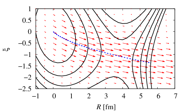
To make a further comparison of the tunneling path, we compute the flux, =, from the resonance wave function as,
| (15) |
and
| (16) |
The flux is shown in Fig. 6 and is compared to the semi-classical escape path. The quantum flow is a collection of all the trajectories connecting the region around the origin with the continuum region. We see that the main quantum mechanical flow is systematically parallel to the semi-classic trajectory. The semi-classical path can thus be regarded as the mean trajectory of the quantum flow, where as the quantum flow takes into account the quantum mechanical fluctuation around the classical trajectory.
In addition to the agreement for the tunneling path, we also compare in Fig. 7 the resulting fission life-time. Varying the parameter in the potential , we obtain a range of fission life-time from the characteristic time of the system to a life-time longer than the actual life-time of the 238U nucleus. The quantum mechanical life-time is computed from the imaginary part of the resonance energy, while the life-time in the semi-classical approximation is evaluated using the formula Eq. (11) with the action integral evaluated along the escape path in the imaginary time,
| (17) |
The latter is equivalent to approximating the pre-exponential factor by that for a one-dimensional problem with a cubic potential along the escape path [43]. In the range shown in the figure, a good agreement is found between the two methods, the maximum deviation being up to about 20%. Evidently, the semi-classical method provides a good approximation to the multi-dimensional tunneling problem for this Hamiltonian.

IV Summary
We have presented a full-quantum method to study a decay life-time as well as the tunneling dynamics. To this end, we have introduced a complex absorbing potential, which is effectively equivalent to the outgoing boundary condition, and constructed the bi-orthogonal basis. We have shown that this method provides a good tool to follow the time evolution of a system over a very long time. This enables one to compute the decay life-time from a few fm/ to the order of billion of years. A comparison with the semi-classical approximation has shown a good agreement between the two methods. It has been shown that the average of fissioning flux in a multi-dimensional plane corresponds to the semi-classical tunneling path. For the decay life-time, the two methods yield similar values to one another, where the maximum difference is only about by 20%.
The quantum mechanical method discussed in this paper provides a good alternative to the semi-classical method. It provides an intuitive picture of multi-dimensional quantum tunneling, including the quantum mechanical fluctuation of the classical path. It will also provide a convenient method when a bifurcation of tunneling path is important, e.g., in the presence of a competition of several fission modes. We plan to apply this method, both for dynamics and a determination of resonance state, to more realistic systems using the constrained mean field theory for the potential energy surface and/or the time-dependent generator coordinate method [13, 14, 47]. We will report it in a separate publication.
Acknowledgement
G.S. acknowledges the Japan Society for the Promotion of Science for the JSPS postdoctoral fellowship for foreign researchers. This work was supported by Grant-in-Aid for JSPS Fellows No. 14F04769.
References
- [1] M. Brack, J. Damgaard, A.J. Jensen, H.C. Pauli, V.M. Strutinsky, and C.Y. Wong, Rev. Mod. Phys. 44, 320 (1972).
- [2] P. Möller, D.G. Madland, A.J. Sierk, and A. Iwamoto, Nature 409, 785 (2001).
- [3] P. Möller, A.J. Sierk, T. Ichikawa, A. Iwamoto, R. Bengtsson, H. Uhrenholt, and S. Aberg, Phys. Rev. C 79, 064304 (2009).
- [4] J. Skalski, Phys. Rev. C 77, 064610 (2008).
- [5] A. Staszczak, A. Baran, J. Dobaczewski, and W. Nazarewicz, Phys. Rev. C 80, 014309 (2009).
- [6] A. Baran, J.A. Sheikh, J. Dobaczewski, W. Nazarewicz, and A. Staszczak, Phys. Rev. C 84, 054321 (2011).
- [7] J. Sadhukhan, K. Mazurek, A. Baran, J. Dobaczewski, W. Nazarewicz, and J.A. Sheikh, Phys. Rev. C 88, 064314 (2013).
- [8] J.D. McDonnell, W. Nazarewicz, J.A. Sheikh, A. Staszczak, and M. Warda, Phys. Rev. C 90, 021302(R) (2014).
- [9] J. Sadhukhan, J. Dobaczewski, W. Nazarewicz, J. A. Sheikh, and A. Baran, Phys. Rev. C 90, 061304(R) (2014).
- [10] M. Warda and J.L. Egido, Phys. Rev. C 86, 014322 (2012).
- [11] R. Rodriguez-Guzman and L.M. Robledo, Phys. Rev. C 89, 054310 (2014).
- [12] S.A. Giuliani, L.M. Robledo, and R. Rodriguez-Guzman, Phys. Rev. C 90, 054311 (2014).
- [13] H. Goutte, J.F. Berger, P. Casoli, and D. Gogny, Phys. Rev. C 71, 024316 (2005).
- [14] R. Bernard, H. Goutte, D. Gogny, and W. Younes, Phys. Rev. C 84, 044308 (2011).
- [15] H. Abusara, A.V. Afanasjev, and P. Ring, Phys. Rev. C 82, 044303 (2010); Phys. Rev. C 85, 024314 (2012).
- [16] B.-N. Lu, E.-G. Zhao, and S.-G. Zhou, Phys. Rev. C 85, 011301 (2012); Phys. Rev. C 89, 014323 (2014).
- [17] J. Zhao, B.-N. Lu, D. Vretenar, E.-G. Zhao, and S.-G. Zhou, Phys. Rev. C 91, 014321 (2015).
- [18] T. Bürvenich, M. Bender, J. A. Maruhn, and P.-G. Reinhard, Phys. Rev. C 69, 014307 (2004).
- [19] W.D. Myers and W.J. Swiatecki, Nucl. Phys. A601, 141 (1996).
- [20] A. Schmid, Ann. Phys. 170, 333 (1986).
- [21] T. Kindo and A. Iwamoto, Phys. Lett. B225, 203 (1989).
- [22] A. Iwamoto, Z. Phys. A349, 265 (1994).
- [23] N. Carjan, O. Serot, and D. Strottman, Z. Phys. A 349, 353 (1994).
- [24] P. Talou, D. Strottman, and N. Carjan, Phys. Rev. C 60, 054318 (1999).
- [25] D. Lacroix, J.A. Scarpaci, Ph. Chomaz, Nucl. Phys. A 658, 3 (1999).
- [26] T. Maruyama, T. Oishi, K. Hagino, and H. Sagawa, Phys. Rev. C 86, 044301 (2012).
- [27] T. Oishi, K. Hagino, and H. Sagawa, Phys. Rev. C 90, 034303 (2014).
- [28] M. Ueda, K. Yabana, and T. Nakatsukasa, Phys. Rev. C 67, 014606 (2003).
- [29] T. Nakatsukasa and K. Yabana, Phys. Rev. C 71, 024301 (2005).
- [30] P.-G. Reinhard, P. D. Stevenson, D. Almehed, J. A. Maruhn, and M. R. Strayer, Phys. Rev. E 73, 036709 (2006).
- [31] G. Scamps, D. Lacroix, G. F. Bertsch, and K. Washiyama, Phys. Rev. C 85, 034328 (2012).
- [32] J. E. Elenewski and H. Chen, Phys. Rev. B 90, 085104 (2014).
- [33] U.V. Riss and H.-D. Meyer, J. Phys. B26, 4503 (1993).
- [34] S. Feuerbacher, T. Sommerfeld, R. Santra, and L. S. Cederbaum, J. Chem. Phys. 118, 6188 (2003).
- [35] R. Santra, L. S. Cederbaum, J. Chem. Phys. 115, 6853 (2001).
- [36] H. Masui and Y. K. Ho, Phys. Rev. C 65, 054305 (2002).
- [37] M. Ito and K. Yabana, Prog. Theo. Phys. 113, 1047 (2005).
- [38] R. Otani, R. Kageyama, M. Iwasaki, M. Kudo, M. Tomita, and M. Ito, Phys. Rev. C 90, 034316 (2014).
- [39] P. Morse and H. Feshbach, Methods of Theoretical Physics (McGraw-Hill, New York, 1952), p. 884.
- [40] M.S. Hussein, M.P. Pato, and A.F.R. de Toledo Piza, Phys. Rev. C 51, 846 (1995).
- [41] K. Hagino and N. Takigawa, Phys. Rev. C 58, 2872 (1998).
- [42] D.M Brink, M.C. Nemes, D. Vautherin, Ann. Phys. (N.Y.) 147, 171 (1983).
- [43] N. Takigawa, K. Hagino, and M. Abe, Phys. Rev. C 51, 187 (1995).
- [44] S.A. Gurvitz, P.B. Semmes, W. Nazarewicz, and T. Vertse, Phys. Rev. A 69, 042705 (2004).
- [45] D.M. Brink, in The Proceedings of the Peierls 80th Birthday Symposium, A Breadth of Physics, edited by R. H. Dalitz and R. B. Stinchcombe (World Scientific, Singapore, 1988), p. 109.
- [46] A. Baran and K. Pomorski, Nucl. Phys. A 361, 83 (1981).
- [47] P.-G. Reinhard, R.Y. Cusson, and K. Goeke, Nucl. Phys. A398, 141 (1983).