Exploring Hierarchies in Online Social Networks
Abstract
Social hierarchy (i.e., pyramid structure of societies) is a fundamental concept in sociology and social network analysis. The importance of social hierarchy in a social network is that the topological structure of the social hierarchy is essential in both shaping the nature of social interactions between individuals and unfolding the structure of the social networks. The social hierarchy found in a social network can be utilized to improve the accuracy of link prediction, provide better query results, rank web pages, and study information flow and spread in complex networks. In this paper, we model a social network as a directed graph , and consider the social hierarchy as DAG (directed acyclic graph) of , denoted as . By DAG, all the vertices in can be partitioned into different levels, the vertices at the same level represent a disjoint group in the social hierarchy, and all the edges in DAG follow one direction. The main issue we study in this paper is how to find DAG in . The approach we take is to find by removing all possible cycles from such that where is a maximum Eulerian subgraph which contains all possible cycles. We give the reasons for doing so, investigate the properties of found, and discuss the applications. In addition, we develop a novel two-phase algorithm, called Greedy-&-Refine, which greedily computes an Eulerian subgraph and then refines this greedy solution to find the maximum Eulerian subgraph. We give a bound between the greedy solution and the optimal. The quality of our greedy approach is high. We conduct comprehensive experimental studies over 14 real-world datasets. The results show that our algorithms are at least two orders of magnitude faster than the baseline algorithm.
1 Introduction
Social hierarchy refers to the pyramid structure of societies, with minority on the top and majority at the bottom, which is a prevalent and universal feature in organizations. Social hierarchy is also recognized as a fundamental characteristic of social interactions, being well studied in both sociology and psychology [11]. In recent years, social hierarchy has attracted considerable attention and generates profound and lasting influence in various fields, especially social networks. This is because the hierarchical structure of a population is essential in shaping the nature of social interactions between individuals and unfolding the structure of underlying social networks. Gould in [11] develops a formal theoretical model to model the emergence of social hierarchy, which can accurately predict the network structure. By the social status theory in [11], individuals with low status typically follow individuals with high status. Clauset et al. in [8] develop a technique to infer hierarchical structure of a social network based on the degree of relatedness between individuals. They show that the hierarchical structure can explain and reproduce some commonly observed topological properties of networks and can also be utilized to predict missing links in networks. Assuming that underlying hierarchy is the primary factor guiding social interactions, Maiya and Berger-Wolf in [22] infer social hierarchy from undirected weighted social networks based on maximum likelihood. All these studies imply that social hierarchy is a primary organizing principle of social networks, capable of shedding light on many phenomena. In addition, social hierarchy is also used in many aspects of social network analysis and data mining. For instance, social hierarchy can be utilized to improve the accuracy of link prediction [21], provide better query results [15], rank web pages [12], and study information flow and spread in complex networks [1, 2].
In this paper, we focus on social networks that can be modeled by directed graphs, because in many social networks (e.g., Google+, Weibo, Twitter) information flow and influence propagate follow certain directions from vertices to vertices. Given a social network as a directed graph , its social hierarchy can be represented as a directed acyclic graph (DAG). By DAG, all the vertices in are partitioned into different levels (disjoint groups), and all the edges in the cycle-free DAG follow one direction, as observed in social networks that prestige users at high levels are followed by users at low levels and the prestige users typically do not follow their followers. Here, a level in DAG represents the status of a vertex in the hierarchy the DAG represents.
The issue we study in this paper is how to find hierarchy as a DAG in a general directed graph which represents a social network. Given a graph , there are many possible ways to obtain a DAG. First, converting graph into a DAG, by contracting all vertices in a strongly connected component in as a vertex in DAG, does not serve the purpose, because all vertices in a strongly connected component do not necessarily belong to the same level in a hierarchy. Second, a random DAG does not serve the purpose, because it heavily relies on the way to select the vertices as the start to traverse and the way to traverse. Therefore, two random DAGs can be significantly different topologically. Third, finding the maximum DAG of is not only NP-hard but also NP-approximate [14]. The way we do is to find the DAG by removing all possible cycles from following [13]. In [13] Gupte et al. propose a way to decompose a directed graph into a maximum Eulerian subgraph and DAG , such that . Here, all possible cycles in are in , and all edges in do not appear in . We take the same approach to find DAG for a graph by finding the maximum Eulerian subgraph of such that , as given in [13].
Main contributions: We summarize the main contributions of our work as follows. First, unlike [13] which studies a measure between 0 and 1 to indicate how close a given directed graph is to a perfect hierarchy, we focus on the hierarchy (DAG). In addition to the properties investigated in [13], we show that found is representative, exhibits the pyramid rank distribution. In addition, found can be used to study social mobility and recover hidden directions of social relationships. Here, social mobility is a fundamental concept in sociology, economics and politics, and refers to the movement of individuals from one status to another. Second, we significantly improve the efficiency of computing the maximum Eulerian subgraph . Note that the time complexity of the BF-U algorithm [13] is , where and are the numbers of vertices and edges, respectively. Such an algorithm is impractical, because it can only work on small graphs. We propose a new algorithm with time complexity , and propose a novel two-phase algorithm, called Greedy-&-Refine, which greedily computes an Eulerian subgraph in and then refines this greedy solution to find the maximum Eulerian subgraph in where is a very small constant less than 1. The quality of our greedy approach is high. Finally, we conduct extensive performance studies using 14 real-world datasets to evaluate our algorithms, and confirm our findings.
Further related work: Ball and Newman [3] analyze directed networks between students with both reciprocated and unreciprocated friendships and develop a maximum-likelihood method to infer ranks between students such that most unreciprocated friendships are from lower-ranked individuals to higher-ranked ones, corresponding to status theory [11]. Leskovec et al. in [19, 18] investigate signed networks and develop an alternate theory of status in replace of the balance theory frequently used in undirected and unsigned networks to both explain edge signs observed and predict edge signs unknown. Influence has been widely studied [6], finding social hierarchy provides a new perspective to explore the influence given the existence of a social hierarchy.
Eulerian graphs have been well studied in the theory community [9, 10, 5, 7, 20]. For example, in [9], Fleischner gives a comprehensive survey on this topic. In [10], the same author surveys several applications of Eulerian graphs in graph theory. Another closely related concept is super-Eulerian graph, which contains a spanning Eulerian subgraph [5, 7, 20], here a spanning Eulerian subgraph means an Eulerian subgraph that includes all vertices. The problem of determining whether or not a graph is super-Eulerian is NP-complete [7]. Most of these work mainly focus on the properties of Eulerian subgraphs. There are no much related work on computing the maximum Eulerian subgraphs for large graphs. To the best of our knowledge, the only one in the literature is done by Gupte, et al. in [13]. However, the time complexity of their algorithm is ), which is clearly impractical for large graphs.
Organization: In Section 2, we focus on the properties of the social hierarchy found after giving some useful concepts on maximum Eulerian subgraph, and discuss the applications. In Section 3, we discuss an existing algorithm BF-U [13]. In Section 4, we propose a new algorithm DS-U of time complexity , and treat it as the baseline algorithm. We present a new two-phase algorithm GR-U for finding the maximum Eulerian subgraph, as well as its analysis in Section 5. Extensive experimental studies are reported in Section 6. Finally, we conclude this work in Section 7.
2 The Hierarchy
Consider an unweighted directed graph , where and denote the sets of vertices and directed edges of , respectively. We use and to denote the number of vertices and edges of graph , respectively. In , a path represents a sequence of edges such that , for each . The length of path , denoted as , is the number of edges in . A simple path is a path with distinct vertices. A cycle is a path where a same vertex appears more than once, and a simple cycle is a path where the first vertices are distinct while . For simplicity, below, we use and to denote and of , respectively, when they are obvious. For a vertex , the in-neighbors of , denoted as , are the vertices that link to , i.e., , and the out-neighbors of , denoted as , are the vertices that links to, i.e., . The in-degree and out-degree of vertex are the numbers of edges that direct to and from , respectively, i.e., and .
A strongly connected component () is a maximal subgraph of a directed graph in which every pair of vertices and are reachable from each other.
A directed graph is an Eulerian graph (or simply Eulerian) if for every vertex , . An Eulerian graph can be either connected or disconnected. An Eulerian subgraph of a graph is a subgraph of , which is Eulerian, denoted as . The maximum Eulerian subgraph of a graph is an Eulerian subgraph with the maximum number of edges, denoted as . Given a directed graph , we focus on the problem of finding its maximum Eulerian subgraph, , which does not need to be connected. Note that the problem of finding the maximum Eulerian subgraph () in a directed graph can be solved in polynomial time, whereas the problem of finding the maximum connected Eulerian subgraph is NP-hard [4]. The following example illustrates the concept of maximum Eulerian subgraph.

Example 2.1.
Fig. 1 shows a graph with 14 vertices and 22 edges. Its maximum Eulerian subgraph is a subgraph of , where its edges are in solid lines: , and is the set of vertices that appear in .
The main issue here is to find a hierarchy of a directed graph as DAG by finding the maximum Eulerian subgraph for a directed graph . With found, can be efficiently found due to , and . We discuss the properties of the hierarchy and the applications.
The representativeness: The maximum Eulerian subgraph for a general graph is not unique. A natural question is how representative is as the hierarchy. Note that is only unique w.r.t found. Below, we show identified by an arbitrary is representative based on a notion of strictly-higher defined between two vertices in , over a ranking where for each edge . Here, for two vertices and , a larger rank implies a vertex is in a higher status in a follower relationship, and is strictly-higher than if and is reachable from , i.e. there is a directed path from to in .
Theorem 2.2.
Let and be two DAGs for such that . There are no vertices and such that is strictly-higher than in whereas is strictly-higher than in .
Proof Sketch: Assume the opposite. We can construct an auxiliary graph . Then finding the maximum Eulerian subgraph for can be done in two steps. In the first step, find the maximum Eulerian subgraph , and in the second step, find the maximum Eulerian subgraph for plus the additional edge . Since , there are supposed to be at least two corresponding relaxing orders, when the first phase terminates, namely, identifying and . For one relaxing order, we can show that the added edge can be relaxed, which results in finding such that . For the other relaxing order, we can also show that the added edge cannot be relaxed and . It leads to a contradiction, because it can find two different maximum Eulerian subgraphs for with different sizes.
Alternatively, let the ranking in and be and . Assume there are two vertices and such that is strictly-higher than by whereas is strictly-higher than by . We prove this cannot achieve based on the finding in [13]. In [13], it gives a total score on which measures how is different from DAG based on a ranking . The total score, denoted as , is obtained by summing up the weights assigned to edges, for edge . The finding in [13] is that the minimum total score equals to the number of edges in the maximum Eulerian subgraph, . Choose and satisfying that and . Since is strictly-higher than in , there is a directed path from to in . We can construct an auxiliary graph , then . On the other hand, over the same , since is strictly-higher than in , we can show , which leads to a contradiction.
A case study: With the hierarchy (DAG ) found, suppose we assign every vertex a minimum non-negative rank such that for any edge , where is a strictly-higher rank. To show whether such ranking reflects the ground truth, as a case study, we conduct testing using Twitter, where the celebrities are known, for instance, refer to Twitter Top 100 (http://twittercounter.com/pages/100). We sample a subgraph among 41.7 million users (vertices) and 1.47 billion relationships (edges) from Twitter social graph crawled in 2009 [16]. In brief, we randomly sample 5 vertices in the celebrity set given in Twitter, and then sample 1,000,000 vertices starting from the 5 vertices as seeds using random walk sampling [17]. We construct an induced subgraph of the 1,000,000 vertices sampled from , and we uniformly sample about 10,000,000 edges from to obtain the sample graph , which contains 759,105 vertices and 11,331,061 edges. In , we label a vertex as a celebrity, if is a celebrity and has at least 100,000 followers in . There are 430 celebrities in including Britney Spears, Oprah Winfrey, Barack Obama, etc. We compute the hierarchy () of using our approach and rank vertices in . The hierarchy reflects the truth: 88% celebrities are in the top 1% vertices and 95% celebrities in the top 2% vertices. In consideration of efficiency, we can approximate the exact hierarchy with a greedy solution obtained by Greedy in Section 5. In the approximate hierarchy, 85% celebrities are in the top 1% vertices and 93% celebrities in the top 2% vertices.


The pyramid structure of rank distribution is one of the most fundamental characteristics of social hierarchy. We test the social networks: wiki-Vote, Epinions, Slashdot0902, Pokec, Google+, Weibo. The details about the datasets are in Table 1 and Table 3. The rank distribution derived from hierarchy , shown in Fig. 2(a), indicates the existence of pyramid structure, while the rank distributions derived from a random DAG (Fig. 2(b)) and by contracting s (Fig. 2(c)) are rather random. Here, the x-axis is the rank where a high rank means a high status, and the y-axis is the percentage in a rank over all vertices. By analyzing the vertices, , in over the difference between in-degree and out-degree, i.e. , it reflects the fact that those vertices with negative are always at the bottom of , whereas those vertices in the higher rank are typically with large positive values.
The social mobility: With the DAG found, we can further study social mobility over the social hierarchy represents. Here, social mobility is a fundamental concept in sociology, economics and politics, and refers to the movement of individuals from one status to another. It is important to identify individuals who jump from a low status (a level in ) to a high status (a level in ). We conduct experimental studies using the social network Google+ (http://plus.google.com) crawled from Jul. 2011 to Oct. 2011 [27, 26], and Sina Weibo (http://weibo.com) crawled from 28 Sep. 2012 to 29 Oct. 2012 [24]. For Google+ and Weibo, we randomly extract 100,000 vertices respectively, and then extract all edges among these vertices in 4 time intervals during the period the datasets are crawled, as shown in Table 1.
| Graph | ||||
|---|---|---|---|---|
| Gplus0 | 100,000 | 115,090 | 2,833 | 6,271 |
| Gplus1 | 100,000 | 512,281 | 14,797 | 70,537 |
| Gplus2 | 100,000 | 2,867,781 | 51,605 | 770,854 |
| Gplus3 | 100,000 | 8,289,203 | 87,941 | 3,644,147 |
| Weibo0 | 100,000 | 2,431,525 | 96,765 | 850,136 |
| Weibo1 | 100,000 | 2,446,002 | 96,833 | 855,131 |
| Weibo2 | 100,000 | 2,463,050 | 96,902 | 861,729 |
| Weibo3 | 100,000 | 2,479,140 | 96,969 | 868,044 |
We show social mobility in Fig. 3. We compare two snapshots, and , and investigate the social mobility from to . For Google+, and are Gplus0 and Gplus1, and for Weibo, and are Weibo0 and Weibo1. For , we divide all vertices into 5 equal groups. The top 20% go into group 5, and the second 20% go to group 4, for example. In Fig. 3, the x-axis shows the 5 groups for . Consider the number of vertices in a group as 100%. In Fig. 3, we show the percentage of vertices in one group moves to another group in . Fig. 3(a) and Fig. 3(b) show the results for Google+ and Weibo. Some observations can be made. Google+ is a new social network when crawled since it starts from Jun. 29, 2011, and Weibo is a rather mature social network since it starts from Aug. 14, 2009. From Fig. 3(a), many vertices move from one status to another, whereas from Fig. 3(b), only a very small number of vertices move from one status to another. Similar results can be observed from approximate hierarchies, by our greedy solution Greedy given in Section 5, as shown in Fig. 3(c) and Fig. 3(d). Those moved to/from the highest level deserve to be investigated.


Recovering the hidden directions is to identify the direction of an edge if the direction of the edge is unknown [25]. The directionality of edges in social networks being recovered is important in many social analysis tasks. We show that our approach has advantage over the semi-supervised approach (SM-ReDirect) in [25]. Here, the task is using the given 20% directed edges as training data to recover the directions for the remaining edges. In our approach, we construct a graph from the 20% training data, and identify by . With the ranking over the vertices, we predict the direction of an edge is from to if . Take Slashdot and Epinion datasets used [25], our approach outperforms the matrix-factorization based SM-ReDirect both in terms of accuracy and efficiency. For Slashdot, our prediction accuracy is 0.7759 whereas SM-ReDirect is 0.6529. For Epinion, ours is 0.8285 whereas SM-Redirect is 0.7118. Using approximate hierarchy, our accuracy is 0.7682 for Slashdot and 0.8277 for Epinion, respectively.
Input: A graph
Output: Two subgraphs of , and ()
3 The Existing Algorithm
To find the maximum Eulerian subgraph, Gupte, et al. in [13] propose an iterative algorithm based on the Bellman-Ford algorithm, which we call BF-U (Algorithm 1). Let be a weight assigned to an edge in . Initially, BF-U assigns an edge-weight with a value of -1 to every edge in graph (Line 1). Let a negative cycle be a cycle with a negative sum of edge weights. In every iteration (Lines 2-7), BF-U finds a negative cycle repeatedly until there are no negative cycles. For every edge in the negative cycle found, it changes the weight of to be and reverses the direction of the edge (Lines 4-5). As a result, it finds a maximum Eulerian subgraph and a directed acyclic graph (DAG) of , denoted as , such that . Since the number of edges with weight +1 increases by at least one during each iteration, there are at most iterations (Line 2-7). In every iteration it has to invoke the Bellman-Ford algorithm to find a negative cycle (Line 2), or to determine whether there is a negative cycle. The time complexity of Bellman-Ford algorithm is . Therefore, in the worst case, the total time complexity of BF-U is , which is too expensive for real-world graphs.
Input: A graph
Output: Two subgraphs of , and ()
4 A New Algorithm
To address the scalability problem of BF-U, we propose a new algorithm, called DS-U. Different from BF-U which starts by finding a negative cycle using the Bellman-Ford algorithm in every iteration, DS-U finds a negative cycle only when necessary with condition. In brief, in every iteration, when necessary, DS-U invokes an algorithm FindNC (short for find a negative cycle) to find a negative cycle while relaxing vertices following DFS order. Applying amortized analysis [23], we prove the time complexity of DS-U, is to find the maximum Eulerian subgraph .
The DS-U algorithm is outlined in Algorithm 2, which invokes FindNC (Algorithm 3) to find a negative cycle. Here, FindNC is designed based on the same idea of relaxing edges as used in the Bellman-Ford algorithm. In addition to edge weight , we use three variables for every vertex , , , and . Here, is a Boolean variable indicating whether there are out-going edges from that may need to relax to find a negative cycle. It will try to relax an edge from further when . When relaxing from , records the next vertex in (maintained as an adjacent list) for the edge to be relaxed next. It means that all edges from to any vertex before has already been relaxed. is an estimation on the vertex which decreases when relaxing. When decreases, is reset to be and is reset to be 0, since all its out-going edges can be possibly relaxed again. Initially, in DS-U, every edge weight is initialized to -1, and the three variables, , , and , on every vertex are initialized to , , and , respectively. All , , , and are used in FindNC to find a negative cycle following the main idea of Bellman-Ford algorithm in DFS order. A negative cycle, found by FindNC while relaxing edges, is maintained using a vertex stack and an edge stack together with a variable , where maintains the first vertex of a negative cycle. In DS-U, by popping vertex/edges from / until encountering the vertex in , a negative cycle can be recovered. As shown in Algorithm 2, in the while statement (Lines 3-15), for every vertex in , only when there is a possible relax () and there is a negative cycle found by the algorithm FindNC, it will reverse the edge direction and update the edge weight, , for each edge in the negative cycle (Lines 6-13).

Example 4.1.
We explain DS-U (Algorithm 2) using an example graph in Fig. 4. For ever vertex , there is an adjacent list to maintain its out-neighbors. Initially, for every vertex , ; and for every edge , . Suppose we process in such an order. In the first iteration, and FindNC () returns true, which implies a negative cycle is found. Here, for all vertices in , we have ; ; ; ; . In addition, , , . Following Lines 6–13 in Algorithm 2, we find and reverse negative cycle and make . In the second iteration, the out-neighbors of are relaxed from in ’s adjacent list, i.e. from edge . FindNC () returns false. We have, , and . In the following iterations (FindNC (), FindNC (), and FindNC ()), all return false. Finally, for vertex , since , FindNC () is unnecessary, and DS-U () terminates. It finds the maximum Eulerian subgraph .
Lemma 4.2.
In Algorithm 2, if there is a negative cycle , holds for at least one vertex .
Proof Sketch: Assume the opposite, i.e., there exists a negative cycle such that for every vertex , . Let , then . Since holds for , then . It leads to a contradiction, if summing both sides from to , then .
Theorem 4.3.
Algorithm 2 correctly finds the maximum Eulerian subgraph when it terminates.
Proof Sketch: It can be proved by Lemma 4.2.
Lemma 4.4.
Given an Eulerian graph , when DS-U () terminates, for each vertex , , where .
Proof Sketch: We do mathematical induction on the maximum number of cycles the Eulerian graph contains.
- 1.
If contains only one cycle, i.e. is a simple cycle itself, it is easy to see that for each vertex , .
- 2.
Assume Lemma 4.4 holds when contains no more than cycles, we prove it also holds when contains at most cycles. We first decompose into a simple cycle which is the last negative cycle found during DS-U () and the remaining is an Eulerian graph containing at most cycles. We explain the validation of this decomposition as follows. If the last negative cycle found contains some positive edges, then the resulting maximum Eulerian subgraph will contain some negative edges, it is against the fact that itself is given as Eulerian. Next, we decompose DS-U () into two phases, it finds as an Eulerian subgraph in the first phase while cycle is identified in the second phase. According to the assumption, when the first phase completes, for each vertex , where is by DS-U () and is the result by relaxing . There are two cases for the second phase.
- (a)
If , the two phases are independent. Therefore, when the second phase terminates, for each vertex , , and for each vertex , , Lemma 4.4 holds.
- (b)
If , suppose , then when the first phase completes. During the second phase, decreases by , then . For any vertex , can only change along a path , where and , for . Then . Therefore, Lemma 4.4 holds.
- (a)

Example 4.5.
We explain the proof of 2(b) in Lemma 4.4 using Fig. 5. Fig. 5 shows an Eulerian graph containing simple cycles. Suppose the first negative cycle found is , with the resulting . In a similar way, suppose the second negative cycle found is by relaxing , and the third negative cycle is with . By reversing these three negative cycles, we have a cycle , and a graph which is a simple cycle with . As can be seen, the current is in the range of . When DS-U () terminates, is in the rage of , and is in the range of . It shows that Lemma 4.4 holds for this example.
Lemma 4.6.
Given a general graph , when DS-U () terminates, for each vertex , , where .
Proof Sketch: For a general graph , we can add edges from vertices with to vertices with and . Obviously, the resulting augment graph has at most edges.
Based on Lemma 4.4, when DS-U () terminates, each vertex satisfies . On the other hand, DS-U () can be decomposed into two phases, DS-U () and further relaxations exploiting , implying that for each vertex , holds when DS-U () terminates.
Lemma 4.7.
For each value of of every vertex , the out-neighbors of , i.e. , are relaxed at most once.
Proof Sketch: As shown in Algorithm. 3, is monotone decreasing, and is monotone increasing for a particular value. So Lemma 4.7 holds.
Theorem 4.8.
Time complexity of DS-U () is .
Proof Sketch: Given Lemma 4.4, Lemma 4.6, and Lemma 4.7, since every edge is checked at most times for relaxations. By applying amortized analysis [23], the time complexity of DS-U () is .
Consider Algorithm 2. During each iteration of the while loop, only a small part of the graph can be traversed and most edges are visited at most twice. Therefore, each iteration can be approximately bounded as , and the time complexity of DS-U is approximated as , where is the number of iterations, bounded by . In the following discussion, we will analyze the time complexity of algorithms based on the number of iterations.
5 The Optimal: Greedy-&-Refine
DS-U reduces the time complexity of BF-U to , but it is still very slow for large graphs. To further reduce the running time of DS-U, we propose a new two-phase algorithm which is shown to be two orders of magnitude faster than DS-U. Below, we first introduce an important observation which can be used to prune many unpromising edges. Then, we will present our new algorithms as well as theoretical analysis.
Let be a set of strongly connected components (s) of , such that , where is an of , , and for . We show that for any edge, if it is not included in any of , then it cannot be contained in the maximum Eulerian subgraph . Therefore, the problem of finding the maximum Eulerian subgraph of becomes a problem of finding the maximum Eulerian subgraph of each , since the union of the maximum Eulerian subgraph of , , is the maximum Eulerian subgraph of .
Lemma 5.1.
An Eulerian graph can be divided into several edge disjoint simple cycles.
Proof Sketch: It can be proved if there is a process that we can repeatedly remove edges from a cycle found in an Eulerian graph , and has no edges after the last cycle being removed. Note that for every in . Let a subgraph of , denoted as , be such a cycle found in . is an Eulerian subgraph, and is also an Eulerian subgraph. The lemma is established.
Theorem 5.2.
Let be a directed graph, and be a set of s of . The maximum Eulerian subgraph of , .
Proof Sketch: For each edge , there is at least one cycle containing this edge, given by Lemma 5.1. Therefore, and belong to the same , i.e., for any edge , it cannot be included in . The theorem is established.
Below, we discuss how to find the maximum Eulerian subgraph for each strongly connected component () of . In the following discussion, we assume that a graph is an itself.
We can use DS-U to find the maximum Eulerian subgraph for an . However, DS-U is still too expensive to deal with large graphs. The key issue is that the number of iterations in DS-U (Algorithm 2, Lines 3-15), can be very large when the graph and its maximum Eulerian subgraph are both very large. Since in most iterations, the number of edges with weight +1 increases only by 1, and thus it takes almost iterations to get the optimal number of edges in the maximum Eulerian subgraph .
In order to reduce the number of iterations, we propose a two-phase Greedy-&-Refine algorithm, abbreviated by GR-U. Here, a Greedy algorithm computes an Eulerian subgraph of , denoted as , and a Refine algorithm refines the greedy solution to get the maximum Eulerian subgraph , which needs at most iterations. The GR-U algorithm is given in Algorithm 4, and an overview is shown in Fig. 6. In Algorithm 4, it first computes all s (Line 1). For each , it computes an Eulerian subgraph using Greedy, denoted as (Line 3). In Greedy, in every iteration (), it identifies a subgraph by an -Subgraph algorithm, and further deletes/reverses all specific length- paths called -s which we will discuss in details by DFS. Note is a small number. After computing , is near acyclic, and it moves all cycles from to (Line 4). Finally, it refines to obtain the optimal by calling Refine (Line 5). The union of all is the maximum Eulerian subgraph for . Below, we first list some important concepts introduced in the algorithm and analysis parts in Table. 2, and then we shall detail the greedy algorithm and refine algorithm, respectively.
| Used-In | Symbol | Meaning |
|---|---|---|
| Greedy | ||
| - | path, , , and for | |
| (-Subgraph) subgraph of contains all -s of length | ||
| , | ||
| the shortest distance from any vertex with a positive label, , in | ||
| the shortest distance to any vertex with a negative label, , in | ||
| Refine | , , , and | |
| Analysis | -/- | a path where every edge is with a positive/negative weight |
| - | , where are -s, and plus are -s | |
| the total weight of -s for a - () | ||
| the total weight of -s for a - () | ||
| , and |

5.1 The Greedy Algorithms
Given a graph , we propose two algorithms to obtain an initial Eulerian subgraph . The first algorithm is denoted as Greedy-D (Algorithm 5), which deletes edges from to make for every vertex in . The second algorithm is denoted as Greedy-R (Algorithm 8), which reverses edges instead of deletion to the same purpose. We use Greedy when we refer to either of these two algorithms. By definition, the resulting is an Eulerian subgraph of . The more edges we have in , the closer the resulting subgraph is to . We discuss some notations below
The vertex label: For each vertex in , we define a vertex label on , . If , it means that can be a vertex in an Eulerian subgraph without any modifications. If , it needs to delete/reverse some adjacent edges to make being zero.
The pn-path: We also define a positive-start and negative-end path between two vertices, and , denoted as - . Here, - is a path , where and with the following conditions: , , and all for . Clearly, by this definition, if we delete all the edges in - , then decreases by 1, increases by 1, and all intermediate vertices in - will have their labels as zero. To make all vertex labels being zero, the total number of such -s to be deleted/reversed is .
The transportation graph : A transportation graph of is a graph such that and .
The and : is the shortest distance from any vertex with a positive label, , in . is the shortest distance from any vertex with a positive label, , in . Note is the shortest distance to any vertex with a negative label, , in .
5.1.1 The Greedy-D Algorithm
Below, we first concentrate on Greedy-D (Algorithm 5). Let be (Line 1). In the while loop (Lines 2-4), it repeatedly deletes all -s starting from length by calling an algorithm PN-path-D (Algorithm 6) until no vertex in with a positive value ().

Example 5.3.
Consider graph in Fig. 7. Three vertices, , , and , in double cycles, have a +1, and three other vertices, , , and , in dashed cycles, have a -1. Initially, , Greedy-D (Algorithm 5) deletes - , making . When , - is deleted. Finally, when , - will be deleted. In Fig. 7, the graph with solid edges is or the graph returned by Algorithm 5. It is worth mentioning that for the same graph , DS-U needs 10 iterations. From the Eulerian subgraph obtain by Greedy, it only needs at most 2 additional iterations to get the maximum Eulerian subgraph.
It is worth noting that is not optimal. Some edges in may not be in the maximum Eulerian subgraph, while some edges deleted should appear in the maximum Eulerian subgraph. In next section, we will discuss how to obtain the maximum Eulerian subgraph from the greedy solution .
Finding all pn-paths with length : The PN-path-D algorithm is shown in Algorithm 6. In brief, for a given graph , PN-path-D first extracts a subgraph which contains all -s of length that are possible to be deleted from by calling an algorithm -Subgraph (Algorithm 7) in Line 1. In other words, all edges in but not in cannot appear in any -s with a length . Based on obtained, PN-path-D deletes -s from (not from ) with additional conditions (in Lines 2-13). Let be a subgraph of that includes all edges appearing in -s of length to be deleted in PN-path-D. PN-path-D will return a subgraph as a subgraph of , which will be used in the next run in Greedy-D for deleting -s with length .
We discuss the -Subgraph algorithm (Algorithm 7), which extracts from by BFS (breadth-first-search) traversing twice. In the first BFS (Lines 4-6), it adds a virtual vertex , and adds an edge to every vertex with a positive label () in . Then, it assigns a to every vertex in as follows. Let be . By BFS, it assigns to be , where is the parent vertex of following BFS. In the second BFS (Lines 7-10), it conceptually considers the transposition graph of by reversing every edge as (Line 7). Then, it assigns a different to every vertex in using the transposition graph . Like the first BFS, it adds a virtual vertex , and adds an edge to every vertex with a negative label () in . Then, it assigns to every vertex in as follows. Let be . By BFS, it assigns to be , where is the parent vertex of in following BFS. The resulting subgraph to be returned from -Subgraph is extracted as follows. Here, contains all vertices in if for the given length , and contains all edges if both and appear in , is an edge in the given graph , and (Lines 11-13). The following example illustrates how -Subgraph algorithm works.


Example 5.4.
Fig. 9 illustrates the returned by -Subgraph (Algorithm 7) when . It is constructed using two BFS, i.e., BFS () and BFS (), and the associated BFS-trees with level and are shown in Fig. 8(a) and Fig. 8(b), respectively. In Fig. 8(a), vertices and are the only vertices with . In Fig. 8(b), vertex is the only one with . Therefore, contains only four edges, in dashed lines, which is much smaller than the original graph to be handled.
Lemma 5.5.
By -Subgraph, the resulting subgraph includes all -s of length in .
Proof Sketch: Recall that -Subgraph returns a graph where and . It implies the following. All vertices in are on at least one shortest path from a positive label vertex () to a negative label vertex () of length . All edges are on such shortest paths. No any edge in a - of length will be excluded from . In other words, there does not exist an edge on - of length , which does not appear in .
We explain PN-path-D (Algorithm 6). Based on obtained from using -Subgraph (Algorithm 7), in PN-path-D, we delete all possible -s of length from (Lines 2-13). The deletion of all -s of length from the given graph is done using DFS over with a queue . It first pushes all vertices in with a positive label () into queue , because they are the starting vertices of all -s with length . We check the vertex on the top of queue . With the vertex , we do DFS starting from over , traverse unvisited edges in , and mark the edges visited as “visited”. Let be the first - with length along DFS. We delete all edges on , and adjust the labels as to reduce by 1 and increase by 1. We dequeue from queue until we cannot find any more -s of length starting from , i.e. returned by DFS is empty. It is important to note that we only visit each edge at most once. There are two cases. One is that the edges visited will be deleted and there is no need to revisit. The other is that they are marked as “visited” but not included in any -s with length . For this case, these edges will not appear in any other -s starting from any other vertices.
Lemma 5.6.
By PN-path-D, all -s of length are deleted.
Proof Sketch: It can be proved based on DFS over obtained from -Subgraph.
Lemma 5.7.
By PN-path-D, the resulting does not include any -s of length .
Proof Sketch: Let be the resulting graph of PN-path-D after deleting all -s of length from . It is trivial when . Assume that it holds for when . We prove that holds when . First, there are no -s of length in graph as a result of PN-path-D by assumption. Second, because is obtained by deleting -s of length from , as given in the Greedy-D algorithm (Algorithm 5). Furthermore, in PN-path-D, every vertex with in keeps in . If there is a - of length found in , then it must be in , which contradicts the assumption. Therefore, does not include any -s of length .
Theorem 5.8.
The PN-path-D algorithm correctly identifies a subgraph which contains all -s of length and returns a graph includes no -s of length .
We discuss the time complexity of the Greedy-D algorithm. In our experiments, we show that more than 99.99% -s deleted in most real-world datasets are with a length less than or equal to 6. We take the maximum length in the Greedy-D algorithm, which is equivalent to the iterations of calling PN-path-D, as a constant, since it is always less than 100 in our extensive experiments. Here, both PN-path-D and -Subgraph cost , because -Subgraph invokes BFS twice and PN-path-D performs DFS once in addition. Given as a constant, the time complexity of the Greedy-D algorithm is .
5.1.2 The Greedy-R Algorithm
The Greedy-R algorithm is shown in Algorithm 8. Like Greedy-D, Greedy-R will result in an Eulerian subgraph. Unlike Greedy-D, it reverses the edges on -s of length from until there does not exist a vertex in with . Initially, Greedy-R assigns every edge, , in with a weight . Then, in the while loop, it calls PN-path-R. PN-path-R is the same as PN-path-D (Algorithm 6) except that in Algorithm 6 Line 7 is changed to be “reverse all edges in - in , both weights and directions”. As a result, Greedy-R identifies an Eulerian subgraph of , . Here, contains all edges with a weight and contains all the vertices in . Below, we give two lemmas to prove the correctness of Greedy-R.
Lemma 5.9.
By PN-path-R, the resulting does not include any -s of length .
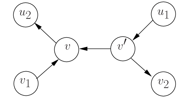
Proof Sketch: Let be the resulting graph of PN-path-R , i.e. after reversing all -s of length from . It is trivial when . Assume that it holds for when . We prove that holds when . Otherwise, suppose that there is a - of length in , then there exists at least one edge in - that has been reversed during PN-path-R , otherwise, - will be fully included in . Without loss of generality, assume that edge is a part of - of length . Fig. 10 shows (before calling PN-path-R ). Then, we can easily construct - and - , and at least one of them is of length , contradicting the assumption. In addition, there can not exist any - of length in . As a consequence, by PN-path-R, the resulting does not include any -s of length .
Similar to Theorem. 5.8, PN-path-R algorithm correctly identifies a subgraph which contains all -s of length and returns a graph includes no -s of length .
Theorem 5.10.
The PN-path-R algorithm correctly identifies a subgraph which contains all -s of length and returns a graph includes no -s of length .
We omit the proof of Theorem. 5.10 since it can be proved in a similar manner like Theorem. 5.8 using Lemma 5.9.


It is worth noticing that obtained by Greedy-R is at least as good as that obtained by Greedy-D. If each edge in is reversed once, then the obtained by Greedy-R is equivalent to that obtained by Greedy-D, as each edge appears in at most one -. On the other hand, if there are some edges being reversed more than once, Greedy-R performs better. Fig. 11 shows the difference between Greedy-D and Greedy-R. Since -s of length 1 and 2 are the same, we only show the last deleted/reversed -. In Fig. 11(a), we delete - . On the other hand, in Fig. 11(b), we reverse - . Here edge is reversed twice. returned by Greedy-R consists of solid lines, which is better than that returned by Greedy-D.
5.2 The Refine Algorithm
With the greedy Eulerian subgraph found, we have insight on because we know where is a DAG (acyclic), and can design a Refine algorithm based on such insight, to reduce the number of times to update , which reduces the cost of relaxing. The Refine algorithm (Algorithm 9) is designed based on the similar idea given in DS-U using FindNC with two following enhancements.
Input: A graph , and the Eulerian subgraph obtained by Greedy,
Output: Two subgraphs of , and ()
First, we utilize to initialize the edge weight for every edge and for every vertex in . The edge weights are initialized in Line 1-7 in Algorithm 9 based on which is a greedy Eulerian subgraph. We also make use of to initialize based on Eq. (1) in Line 8.
| (1) |
Some comments on the initialization are made below. Following Algorithm 2, can be initialized as . In fact, consider Lemma 4.2. No matter what is for a vertex () in a negative cycle , the negative cycle can be identified because there is at least one edge that can be relaxed. Based on it, if we initialize in a way such that , then cannot be relaxed through before updating . It reduces the number of times to update , and improves the efficiency. We explain it further. Because for any edge, , can never be relaxed through edge before being updated, FindNC () will relax edges along a path with a few branches to identify a -. The variables such as and are initialized in Line 9 as done in Algorithm 2.
Second, we use a queue to maintain candidate vertices, , from which there may exist -s, if . Initially, all vertices are enqueued into . In each iteration, when invoking FindNC (), let be the set of vertices relaxed. Among , for any vertex , has been updated and it has only relaxed partial out-neighbors when finding the negative cycle. On the other hand, for any vertex , all of the out-neighbors of have been relaxed and cannot be relaxed before updating . We exclude from implicitly by setting in FindNC ().
Example 5.11.
Suppose we have a greedy Eulerian subgraph (Fig. 7) of (Fig. 1) by Greedy-D, and will refine it to the optimal using Refine. Initially, all edges (solid lines) in are reversed with initial +1 edge weight, and all remaining edges in are initialized with -1 edge weight. , and other vertices have . In the while loop, FindNC () relaxes and returns false. This makes by which and are dequeued from . Afterwards, none of can relax any out-neighbors, and all are dequeued from . FindNC () relaxes all vertices, finds a negative cycle , and adds into as new candidates. Then, no vertices from to can relax any out-neighbors until FindNC () finds the last negative cycle . For most cases, FindNC () relaxes a few of ’s out-neighbors.
We discuss the time complexity of Refine. The initialization (Lines 1–9) is . Since approximates , the number of -s found by Refine will be no more than , and vertices will have updated less than times. This implies the while loop costs . Time complexity of Refine is , where , as confirmed in our testing.
5.3 The Bound between Greedy and Optimal
We discuss the bound between obtained by Greedy and the maximum Eulerian subgraph . To simplify our discussion, below, a graph is a graph with multiple edges between two vertices but without self loops, and every edge is associated with a weight , which is initialized to be -1. Given a graph , we use to represent the reversed graph of such that and contains every edge if , and . In addition, we use two operations, and , for two graphs and . Here, is an operation that constructs a new graph by union of two graphs, and , such that , and . And is an operation that constructs a new graph by removing a subgraph from () such that and . Given two Eulerian subgraphs, and , it is easy to show that and are still Eulerian graphs. Given any graph , is an Eulerian graph. Note that assume that there is a cycle with two edges, and , between two vertices, and , in . there will be four edges in , i.e., two edges are from and two corresponding reversed edges from .


We discuss the bound using an Eulerian graph , where and . We call every edge in a negative edge (-), and a path in a negative path (-). We also call every edge in a positive edge (-), and a path in a positive path (-). It is important to note that -s are given for but not for , all -s are with a weight of -1, while all -s are with a weight of +1, because they are the reversed edges in . Here, is a graph with multiple edges between a pair of vertices.
Example 5.12.
Consider the example graph in Fig. 1. The Eulerian subgraph obtained by Greedy, i.e. is shown in Fig. 12(a). It is worth noting that we make use of the resulting graph of Greedy-D, since that obtained by Greedy-R is actually the maximum Eulerian subgraph in this case. Fig. 12(c) shows the maximum Eulerian subgraph . As observed, some edges in do not appear in , while some edges that do not appear in appear in . Fig. 12(b) and Fig. 12(d) show and , respectively. Fig. 13 shows . In Fig. 13, the solid edges represent the -s from , and the dashed edges represent the -s from .
Since is Eulerian, it can be divided into several edge disjoint simple cycles as given by Lemma 5.1. Among these cycles, there are no cycles in with only -s, because they must be in if exist. And there are no cycles in with only -s, because all such cycles have been moved into in GR-U (Algorithm 4, Line 4).
Next, let a cycle be a - if the total weight of the edges in this cycle , and let it be a - if its total weight of edges . We show there are no -s in .
Lemma 5.13.
There does not exist a - in .
Proof Sketch: Assume there is a - in , denoted as . Since there are no cycle with only -s or -s, there are -s and -s in . We divide into two subgraphs, and . Here consists of all -s, where each - is with a +1 weight, and consists of all -s, where each - is with a -1 weight. Clearly, , since it assumes that is a -. Note that , which is equivalent to , is Eulerian, and it contains more edges than , resulting in a contradiction. Therefore, there does not exist a - in .
Lemma 5.13 shows all cycles in are non-negative. Since there are no cycles with only -s or -s, each cycle in can be partitioned into an alternating sequence of -s and -s, and represented as , where , for , are -s, and , for , , plus are -s. We call such cycle a -. Fig. 14(a) shows an example of -, and an arrow presents a path. -s are in solid lines while -s are in dashed lines.


The difference is equal to , becomes the total number of edges in minus the total number of edges in . On the other hand, the difference can be considered as the total weight of all -s in . Recall that all edges in are with weight -1 and the edges in are with weight +1 by our definition. Assume that , where is a -. The total weight of regarding all -s is . Below, we bound using -s.
Consider in Fig. 13, there are 3 -s. and with weight 0, and with weight 2. This means that it needs at most 2 more iterations to get the maximum Eulerian subgraph from the greedy solution.
For a - , we use and to represent the total weight of -s 11 1 For -s, we take the absolute value of total weight. and -s, i.e. and . Because is determined by the optimal in , the bound is obtained when getting the maximum of .


Theorem 5.14.
The upper bound of the total weight of -s in a - with specific is times that of -s, i.e.,
Proof Sketch: The proof is based on the way -s constructed by Greedy-R. For simplicity, we first assume that each - and - is a - itself, and we will deal with general cases later. Based on Greedy-R, a - is constructed as shown in Fig. 15, which is a 4-cycle. Initially, there are -s, , , as Fig. 15(a) shows. Greedy-R deals with -s of length from a small to a large . First, Greedy-R finds a path = - , and combines with two separated -s, and into a new - . Here, is no larger than any . Greedy-R will repeat this process to add all -s, into - in an ascending order of their lengths. The last - to be added to - should be the longest one among all -s. Then its upper bound is . Otherwise, its upper bound should be . Below, we prove Theorem. 5.14.
- •
For 2-cycle (Fig. 14(b)): Since , , and we have,
- •
- •
Assume that it holds for -s when , we prove that it also holds when . Suppose that the shortest - is , combine , and into a single - , then we get a - as . As a result, .
Let and denote the total weight of -s and -s in a - . Bounding - can be formulated as an LP (linear programming) problem.


In Fig. 16(a), at y-axis illustrates the theoretical upper bound of by solving the LP problem, where the three solid lines represent the three conditions in the above LP problem, respectively. Here, is the maximum among all values. The theoretical upper bound is far from tight. First, , which is a tighter upper bound of , moving Cond-3 towards the origin. Second, for most -s, , , since most -s in a - are far from the upper bound it can get. This leads Cond-2 moving towards x-axis. Therefore, a tighter empirical upper bound is at y-axis in Fig. 16(b). We will show it in the experiments.

We have proved Theorem 5.14 for the case -s and -s are -s, which shows that each - in a - has an implicit upper bound. In general, there are cases where -s are not -s. In fact, each - in a - can be classified into two classes. (a) A - is a part of a -, including the case that the - is a -. (b) A - can be divided into several sub-paths, each is a part of a -. In Fig. 17, there are three -s in the -, is a part of - , itself is - and consists of two sub-paths: and , and each of them is a part of a - or itself is a -.
For the cases when a - in a - is not a -, we use and to denote its practical weight and the theoretical upper bound it can reach when itself is a -, respectively. Since we concentrate on weight of -s, we treat such a - as a - with weight if , and treat it as a - with weight if and add the difference to a global variable . We will show in Section 6 that is very small compared with .
Time complexity: Revisit GR-U (Algorithm 4), it includes four parts: decomposition (Line 1), Greedy (Line 3), cycle moving (Line 4) and Refine (Line 5). decomposition can be accomplished in 2 DFS, in time . As analyzed in Section 5, Greedy invokes times PN-path, and each PN-path needs 2 BFS (-Subgraph) and 1 DFS (remove/reverse -s). Since is small ( in our extensive experiments), the time complexity of Greedy is . Regarding moving cycles from to , it is equivalent to moving cycles from non-trivial s of to . Based on the fact that is near acyclic, there are a few cycles in , cycle moving is in . The time complexity of Refine, as given in Section 5.2 is , because most FindNC () relax edges along a path with a few branches and vertices will have updated less than times.
6 Performance Studies
We conduct extensive experiments to evaluate two proposed GR-U algorithms. One is GR-U-D using Greedy-D (Algorithm 5) and Refine (Algorithm 9), and the other is GR-U-R using Greedy-R (Algorithm 8) and Refine (Algorithm 9). We do not compare our algorithms with BF-U in [13], because BF-U is in and is too slow. We use our DS-U as the baseline algorithm, which is . We show that Greedy produces an answer which is very close the the exact answer. In order to confirm Greedy is of time complexity , we show the largest iteration used in Greedy is a small constant by showing that the longest - (the same as ) deleted/reversed by Greedy is small. In addition, we confirm the constant of for Refine is very small by showing statistics of , , and -s. We also confirm the scalability of GR-U as well as Greedy and Refine.
All these algorithms are implemented in C++ and complied by gcc 4.8.2, and tested on machine with 3.40GHz Intel Core i7-4770 CPU, 32GB RAM and running Linux. The time unit used is second.
| Graph | ||||
|---|---|---|---|---|
| wiki-Vote | 7,115 | 103,689 | 1,286 | 17,676 |
| Gnutella | 62,586 | 147,892 | 11,952 | 18,964 |
| Epinions | 75,879 | 508,837 | 33,673 | 264,995 |
| Slashdot0811 | 77,360 | 828,159 | 70,849 | 734,021 |
| Slashdot0902 | 82,168 | 870,159 | 71,833 | 748,580 |
| web-NotreDame | 325,729 | 1,469,679 | 99,120 | 783,788 |
| web-Stanford | 281,903 | 2,312,497 | 211,883 | 691,521 |
| amazon | 403,394 | 3,387,388 | 399,702 | 1,973,965 |
| Wiki-Talk | 2,394,385 | 5,021,410 | 112,030 | 1,083,509 |
| web-Google | 875,713 | 5,105,039 | 461,381 | 1,841,215 |
| web-BerkStan | 685,230 | 7,600,595 | 478,774 | 2,068,081 |
| Pokec | 1,632,803 | 30,622,560 | 1,297,362 | 20,911,934 |
Datasets: We use 14 real datasets. Among the datasets, Epinions, wiki-Vote, Slashdot0811, Slashdot0902, Pokec, Google+, and Weibo are social networks; web-NotreDame, web-Stanford, web-Google, and web-BerkStan are web graphs; Gnutella is a peer-to-peer network; amazon is a product co-purchasing network; and Wiki-Talk is a communication network. All the datasets are downloaded from Stanford large network dataset collection (http://snap.stanford.edu/data) except for Google+ and Weibo. The detailed information of the datasets are summarized in Table 1 and Table 3. In the tables, for each graph, the 2nd and 3rd columns show the numbers of vertices and edges22 2 for each dataset, we delete all self-loops if exist., respectively, and the 4th and 5th columns show the numbers of vertices and edges of its maximum Eulerian subgraph, respectively.
| Graph | Refine | GR-U-D | Refine | GR-U-R | DS-U | |
|---|---|---|---|---|---|---|
| wiki-Vote | 0.1 | 0.1 | 0.1 | 0.1 | 1.0 | 0.100 |
| Gnutella | 0.5 | 0.5 | 0.4 | 0.4 | 1.6 | 0.250 |
| Epinions | 15.9 | 16.1 | 15.2 | 15.4 | 414.4 | 0.037 |
| Slashdot0811 | 80.6 | 80.8 | 70.9 | 71.0 | 12,748.6 | 0.006 |
| Slashdot0902 | 87.3 | 87.5 | 76.6 | 76.8 | 14,324.5 | 0.005 |
| web-NotreDame | 2.6 | 3.0 | 2.4 | 2.7 | 370.4 | 0.007 |
| web-Stanford | 21.5 | 25.7 | 16.7 | 24.9 | 2,780.0 | 0.009 |
| amazon | 126.5 | 133.5 | 124.8 | 130.5 | 44,865.0 | 0.003 |
| Wiki-Talk | 504.3 | 504.9 | 487.3 | 487.9 | 9,120.1 | 0.053 |
| web-Google | 100.2 | 110.3 | 78.6 | 84.6 | 35,271.7 | 0.002 |
| web-BerkStan | 129.7 | 137.7 | 67.8 | 75.9 | 7,853.9 | 0.010 |
| Pokec | 30,954.5 | 30,983.7 | 30,120.4 | 30,140.5 | - | - |
| Gplus2 | 363.5 | 364.2 | 360.5 | 361.2 | 39,083.8 | 0.009 |
| Weibo0 | 206.5 | 207.3 | 202.4 | 203.3 | 8,004.6 | 0.025 |
Efficiency: Table 4 shows the efficiency of these three algorithms, i.e., GR-U-D, GR-U-R, and DS-U, over 14 real datasets. For GR-U-D, the 2nd column shows the running time of Refine and the 3rd column shows the total running time of GR-U-D. As can be seen, for GR-U-D, the running time of Refine dominates that of Greedy-D. The 4th and 5th columns show the running time of Refine and the total running time of GR-U-R, respectively. Likewise, the Refine algorithm is the most time-consuming procedure in GR-U-R. It is important to note that both GR-U-D and GR-U-R significantly outperform DS-U. In most large datasets, GR-U-D and GR-U-R are two orders of magnitude faster than DS-U. For instance, in web-Stanford dataset, GR-U-R takes 25 seconds to find the maximum Eulerian subgraph, while DS-U takes 2,780 seconds, which is more than 100 times slower. In addition, it is worth mentioning that in Pokec dataset, DS-U cannot get a solution in two weeks. In the 6th column, is the value in Refine’s time complexity , by comparing running time of GR-U-R and DS-U. In all graphs, . Note BF-U is very slow, for example, BF-U takes more than 30,000 seconds to handle the smallest dataset wiki-Vote, while our GR-U takes only 0.1 second.

| Graph | IRD | ISD % | IRR | ISR % | IR_DSU |
|---|---|---|---|---|---|
| wiki-Vote | 659 | 95.4 | 629 | 95.6 | 14,361 |
| Gnutella | 2,504 | 69.5 | 1,410 | 82.8 | 8,202 |
| Epinions | 5,466 | 97.4 | 5,334 | 97.4 | 207,124 |
| Slashdot0811 | 11,464 | 97.9 | 9,990 | 98.2 | 541,970 |
| Slashdot0902 | 12,036 | 97.8 | 10,426 | 98.1 | 554,163 |
| web-NotreDame | 9,030 | 98.1 | 6,119 | 98.7 | 486,240 |
| web-Stanford | 23,427 | 94.8 | 15,721 | 96.5 | 448,960 |
| amazon | 75,104 | 94.1 | 61,818 | 95.2 | 1,282,326 |
| Wiki-Talk | 37,662 | 95.7 | 36,139 | 95.9 | 871,020 |
| web-Google | 90,375 | 92.4 | 59,387 | 95.0 | 1,196,616 |
| web-BerkStan | 69,078 | 95.2 | 41,703 | 97.1 | 1,437,188 |
| Pokec | 686,765 | - | 635,286 | - | - |
| Gplus2 | 18,766 | 96.9 | 18,721 | 96.9 | 613,008 |
| Weibo0 | 25,991 | 96.2 | 24,550 | 96.4 | 686,765 |
Effectiveness of Greedy: To evaluate the effectiveness of the greedy algorithms, we first study the size of Eulerian subgraph obtained by Greedy-D and Greedy-R. Fig. 18 depicts the results. In Fig. 18, denotes the size of Eulerian subgraph obtained by the greedy algorithms, denotes the size of the maximum Eulerian subgraph, and denotes the ratio between them. The ratios obtained by both Greedy-D and Greedy-R are very close to 1 in most datasets. That is to say, both Greedy-D and Greedy-R can get a near-maximum Eulerian subgraph, indicating that both Greedy-D and Greedy-R are very effective. The performance of Greedy-R is slightly better than that of Greedy-D, which supports our analysis. The ratio of Gnutella dataset using Greedy-D is slightly lower than others. One possible reason is that Gnutella is much sparser than other datasets, thus some inappropriate - deletions may result in enlarging other -s, and this situation can be largely relieved in Greedy-R.
Second, we investigate the numbers of iterations used in GR-U-D, GR-U-R, and DS-U. Table 5 reports the results. In Table 5, the 2nd and 4th columns ‘IRD’ and ‘IRR’ denote the numbers of iterations used in the refinement procedure (i.e., Refine, Algorithm 9) of GR-U-D and GR-U-R, respectively. The last column ‘IR_DSU’ reports the total number of iterations used in DS-U. From these columns, we can see that in large graphs (e.g., web-NotreDame dataset), the numbers of iterations used in Refine of GR-U-D and GR-U-R are at least two orders of magnitude smaller than those used in DS-U. In addition, it is worth mentioning that in Pokec dataset, DS-U cannot get a solution in two weeks. The 3rd and 5th columns report the percentages of iterations saved by GR-U-D and GR-U-R, respectively. Both Greedy-D and Greedy-R can reduce at least 95% iterations in most datasets. Similarly, the results obtained by GR-U-R are slightly better than those obtained by GR-U-D.
The largest iteration : We show the largest iteration in Greedy by showing the longest -s deleted/reversed, which is the numbers of PN-path-D/PN-path-R invoked by Greedy-D/Greedy-R using the real datasets. Below, the first/second number is the longest -s deleted/reversed. wiki-Vote (9/9), Gnutella (29/22), Epinions (12/10), Slashdot0811 (6/6), Slashdot0902 (8/8), web-NotreDame (96/41), web-Stanford (275/221), amazon (57/37), Wiki-Talk (9/7), web-Google (93/37), web-BerkStan (123/85), Pokec (14/13), Gplus2 (9/8), and Weibo0 (12/10). The longest -s deleted or reversed are always of small size, especially compared with . Therefore, the time complexity of Greedy can be regarded as .
| Graph | |||
|---|---|---|---|
| wiki-Vote | 17,676 | 3,214 | 20 |
| Gnutella | 18,964 | 6,906 | 10 |
| Epinions | 264,995 | 30,997 | 129 |
| Slashdot0811 | 734,021 | 45,315 | 118 |
| Slashdot0902 | 748,580 | 46,830 | 145 |
| web-NotreDame | 783,788 | 10,439 | 3,963 |
| web-Stanford | 691,521 | 35,402 | 6,168 |
| amazon | 1,973,965 | 202,513 | 12,994 |
| Wiki-Talk | 1,083,509 | 158,848 | 331 |
| web-Google | 1,841,215 | 149,425 | 22,361 |
| web-BerkStan | 2,068,081 | 105,569 | 16,991 |
| Pokec | 20,911,934 | 3,003,797 | 8,964 |
| Gplus2 | 770,854 | 117,641 | 80 |
| weibo0 | 850,136 | 124,395 | 384 |

The support to a small : We show the support that given in for Refine is small by giving statistics of , , and -s. We first show the statistics of and discussed in Section 5.3. Table 6 reports the results. From Table 6, we can find that for each graph, and are small compared with . These results confirm our theoretical analysis in Section 5.3. Second, we study the statistics of -s. The results of Epinions and web-Stanford datasets are depicted in Fig. 19, and similar results can be observed from other datasets. In Fig. 19, y-axis denotes the ratio between the total weights of -s and the total weights of -s (i.e., defined in Section 5.3), and the x-axis denotes for -s, where . As can be seen, for all -s, the ratios are always smaller than 2 in both Epinions and web-Stanford datasets. These results confirm our analysis in Section 5.3.


Scalability: We test the scalability for GR-U-R, GR-U-D, and DS-U. We report the results for web-NotreDame and web-Stanford in Fig. 20. Similar results are observed for other real datasets. To test the scalability, we sample 10 subgraphs starting from 10% of edges, up to 100% by 10% increments. Fig. 20(a) and Fig. 20(b) show both GR-U-R and GR-U-D scale well. For web-NotreDame, we further show the performance of Greedy and Refine in Fig. 20(c) and Fig. 20(d). In Fig. 20(c), Greedy seems to be not really linear. We explain the reason below. Revisit Algorithm 4, the efficiency of Greedy is mainly determined by two factors, the graph size (or more precisely the size of the largest ) and the number of times invoking PN-path (i.e. ). When a subgraph is sparse, both size and tend to be small (the smallest sample graph with 10% edges contains a largest with 1,155 vertices and 4,317 edges, and for Greedy-D/Greedy-R), whereas, both the size of the largest and tend to be large in dense subgraphs (the entire graph contains a largest with 53,968 vertices and 296,228 edges, and for Greedy-D/Greedy-R).
7 Conclusion
In this paper, we study social hierarchy computing to find a social hierarchy as DAG from a social network represented as a directed graph . To find , we study how to find a maximum Eulerian subgraph of such that . We justify our approach, and give the properties of and the applications. The key is how to compute . We propose a DS-U algorithm to compute , and develop a novel two-phase Greedy-&-Refine algorithm, which greedily computes an Eulerian subgraph and then refines this greedy solution to find the maximum Eulerian subgraph. The quality of our greedy approach is high which can be used to support social mobility and recover the hidden directions. We conduct extensive experiments to confirm the efficiency of our Greedy-&-Refine approach.
References
- [1] D. Acemoglu, A. Ozdaglar, and A. ParandehGheibi. Spread of (mis) information in social networks. Games and Economic Behavior, 70(2), 2010.
- [2] J. A. Almendral, L. López, and M. A. Sanjuán. Information flow in generalized hierarchical networks. Physica A: Statistical Mechanics and its Applications, 324(1), 2003.
- [3] B. Ball and M. E. Newman. Friendship networks and social status. Network Science, 1(01), 2013.
- [4] L. Cai and B. Yang. Parameterized complexity of evenodd subgraph problems. Journal of Discrete Algorithms, 9(3), 2011.
- [5] P. A. Catlin. Supereulerian graphs: a survey. Journal of Graph theory, 16(2), 1992.
- [6] W. Chen, L. V. Lakshmanan, and C. Castillo. Information and Influence Propagation in Social Networks. Morgan & Claypool, 2013.
- [7] Z. Chen and H. Lai. Reduction techniques for supereulerian graphs and related topics: a survey. Combinatorics and graph theory, 95, 1995.
- [8] A. Clauset, C. Moore, and M. E. Newman. Hierarchical structure and the prediction of missing links in networks. Nature, 453(7191), 2008.
- [9] H. Fleischner. Eulerian graphs and related topics, volume 1. North Holland, 1990.
- [10] H. Fleischner. (some of) the many uses of eulerian graphs in graph theory (plus some applications). Discrete Mathematics, 230(1), 2001.
- [11] R. V. Gould. The origins of status hierarchies: A formal theory and empirical test1. American journal of sociology, 107(5), 2002.
- [12] M. S. Granovetter. The strength of weak ties. American journal of sociology, 1973.
- [13] M. Gupte, P. Shankar, J. Li, S. Muthukrishnan, and L. Iftode. Finding hierarchy in directed online social networks. In Proc. of WWW’11, 2011.
- [14] V. Guruswami, R. Manokaran, and P. Raghavendra. Beating the random ordering is hard: Inapproximability of maximum acyclic subgraph. In Proc. of FOCS’08, 2008.
- [15] J. M. Kleinberg. Authoritative sources in a hyperlinked environment. Journal of the ACM (JACM), 46(5), 1999.
- [16] H. Kwak, C. Lee, H. Park, and S. Moon. What is twitter, a social network or a news media? In Proc. of WWW’10, 2010.
- [17] J. Leskovec and C. Faloutsos. Sampling from large graphs. In Proc. of KDD’06, 2006.
- [18] J. Leskovec, D. Huttenlocher, and J. Kleinberg. Predicting positive and negative links in online social networks. In Proc. of WWW’10, 2010.
- [19] J. Leskovec, D. Huttenlocher, and J. Kleinberg. Signed networks in social media. In Proc. of CHI’10, 2010.
- [20] D. Li, D. Li, and J. Mao. On maximum number of edges in a spanning eulerian subgraph. Discrete mathematics, 274(1), 2004.
- [21] D. Liben-Nowell and J. Kleinberg. The link-prediction problem for social networks. Journal of the American society for information science and technology, 58(7), 2007.
- [22] A. S. Maiya and T. Y. Berger-Wolf. Inferring the maximum likelihood hierarchy in social networks. In Proc. of CSE’09, 2009.
- [23] R. E. Tarjan. Amortized computational complexity. SIAM Journal on Algebraic Discrete Methods, 6(2), 1985.
- [24] J. Zhang, B. Liu, J. Tang, T. Chen, and J. Li. Social influence locality for modeling retweeting behaviors. In Proc. of IJCAI’13, 2013.
- [25] J. Zhang, C. Wang, and J. Wang. Who proposed the relationship?: recovering the hidden directions of undirected social networks. In Proc. of WWW’14, 2014.
- [26] N. Zhenqiang Gong, A. Talwalkar, L. Mackey, L. Huang, E. C. R. Shin, E. Stefanov, D. Song, et al. Jointly predicting links and inferring attributes using a social-attribute network (SAN). ACM Workshop on Social Network Mining and Analysis, 2011.
- [27] N. Zhenqiang Gong, W. Xu, L. Huang, P. Mittal, E. Stefanov, V. Sekar, and D. Song. Evolution of social-attribute networks: Measurements, modeling, and implications using google+. ACM/USENIX Internet Measurement Conference, 2012.