Magnon transport through microwave pumping
Abstract
We present a microscopic theory of magnon transport in ferromagnetic insulators (FIs). Using magnon injection through microwave pumping, we propose a way to generate magnon dc currents and show how to enhance their amplitudes in hybrid ferromagnetic insulating junctions. To this end focusing on a single FI, we first revisit microwave pumping at finite (room) temperature from the microscopic viewpoint of magnon injection. Next, we apply it to two kinds of hybrid ferromagnetic insulating junctions. The first is the junction between a quasi-equilibrium magnon condensate and magnons being pumped by microwave, while the second is the junction between such pumped magnons and noncondensed magnons. We show that quasi-equilibrium magnon condensates generate ac and dc magnon currents, while noncondensed magnons produce essentially a dc magnon current. The ferromagnetic resonance (FMR) drastically increases the density of the pumped magnons and enhances such magnon currents. Lastly, using microwave pumping in a single FI, we discuss the possibility that a magnon current through an Aharonov-Casher phase flows persistently even at finite temperature. We show that such a magnon current arises even at finite temperature in the presence of magnon-magnon interactions. Due to FMR, its amplitude becomes much larger than the condensed magnon current.
pacs
75.30.Ds, 72.25.Mk, 85.75.-dI Introduction
Since the observation of spin-wave spin currents[1] in Y3Fe5O12 (YIG), ferromagnetic insulators (FIs) have been playing a major role in spintronics[2, 3]. All the fascinating features of FIs arise from magnons[4, 5, 6, 7, 8, 9, 10, 11, 12, 13, 14, 15] (i.e., spin-waves), which are bosonic low-energy collective excitations (i.e., quasiparticles) in a magnetically ordered spins system. The use of the magnon degrees of freedom for transport perspectives [8] has led to a new field called magnonics[16, 17].

The main advantages of magnons in FIs can be summarized in the following points: First, transport of magnons in insulating magnets has a lower power absorption compared to electronic conductors[18]. Next, it has been shown experimentally by Kajiwara et al.[1] that magnon currents can carry spin-information over distances of several millimeters, much further than what is typically possible when using spin-polarized conduction electrons in magnetic metals. Third, magnons are quasi-particles (i.e., magnetic excitations) which are not conserved. Then, using microwave pumping[4, 5, 6, 19, 20, 21], they can be directly injected to FIs and their density controlled. A further advantage of magnons arises from the feature that magnons are bosonic excitations and as such they can form a macroscopic coherent[13] state, namely, a quasi-equilibrium Bose-Einstein condensate (BEC)[22, 23, 24, 25]. Demokritov et al.[4] have indeed experimentally shown that such a magnon-BEC can be generated even at room temperature11 1 This proves that low temperatures are not required[47], which may be of crucial importance in view of applications. in YIG by using microwave pumping, and Serga et al.[5] have recently addressed the relation between microwave pumping and the resulting quasi-equilibrium22 2 Regarding the theoretical aspects of their quasi-equilibrium magnon-BECs, see Refs. [23, 24, 25, 48, 49] and also references therein. magnon-BEC (Fig. 1); the applied microwave drives the system into a nonequilibrium steady state[23, 24] and continues to populate the zero-mode of magnons. After switching off the microwaves, the system undergoes a thermalization[19, 26, 27, 28] (or relaxation) process and thereby reaches a quasi-equilibrium state where the pumped magnons form a quasi-equilibrium magnon-BEC[6]. This magnon-BEC is not the ground state but a metastable state[25] that corresponds to a macroscopic coherent precession[23] in terms of spin variables which can last for about 1s.
Motivated by these experimental progress, we microscopically analyzed in Ref. [7] the transport[6] properties in such[4, 5] realized quasi-equilibrium magnon-BECs in FI junctions, and discussed the ac and dc Josephson effects through the Aharonov-Casher (A-C) phase[29], being a special case of a Berry phase [30, 31] in this system. We found that this A-C phase gives a handle to electromagnetically control the Josephson effects and to realize a persistent[32, 33, 12] magnon-BEC current [23, 34, 10, 35] in a ring. An experimental proposal to directly measure this magnon-BEC current also has been theoretically proposed in Ref. [7] through measurements of the induced electric field.
Toward the direct measurement of such magnon currents, one concern[7] might be, however, that the amount of the magnon currents and the resulting electric fields (of the order of V/m) is still[8, 7] very small. This might be an obstacle to the feasibility of such experiments at present.
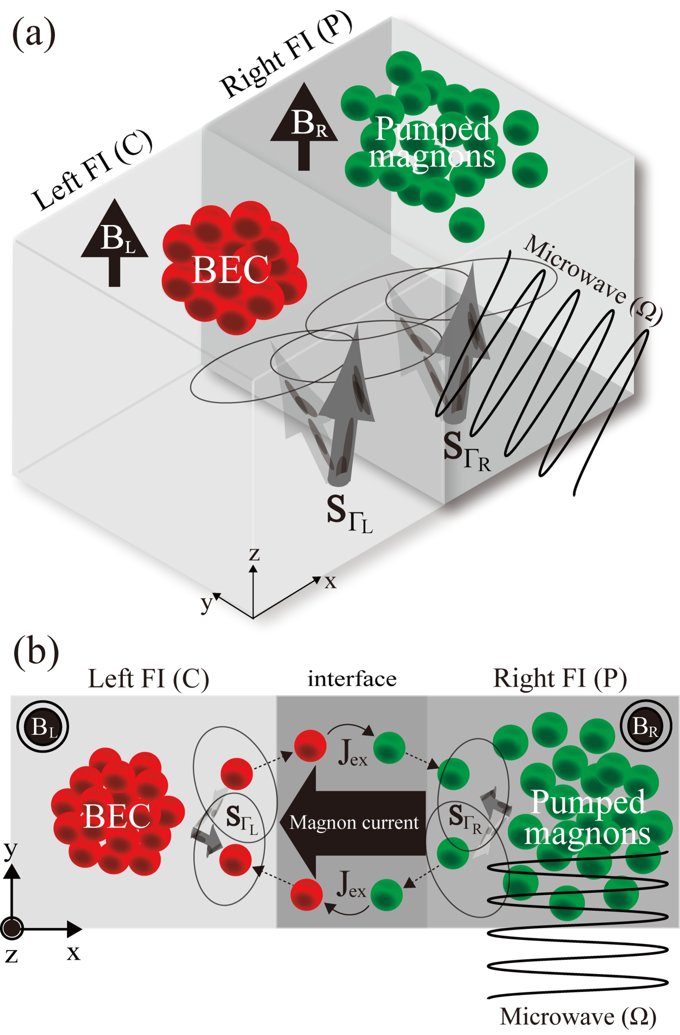
To overcome this problem, we propose to use instead magnon injection through microwave pumping[4, 5, 20] which offers an alternative method to enhance magnon currents in FIs. Because the density of noncondensed magnons is still much larger than that of the magnon condensates in realistic experiments,[4] we consider two kinds of hybrid FI junctions. The first one (Fig. 2) is a junction between quasi-equilibrium magnon condensate and magnons being pumped by microwaves, while the second one (Fig. 5) is a junction between pumped magnons and noncondensed magnons. In order to lighten notations, we denote them as the C-P (Fig. 2) and NC-P (Fig. 5) junctions, with ‘C’ for quasi-equilibrium magnon condensates, ‘P’ for pumped magnons, and ‘NC’ for noncondensed magnons.
This paper is organized as follows. In Sec. II, we first focus on a single FI (P) and microscopically revisit microwave pumping[21, 36] at finite (room) temperature from the viewpoint of magnon injection[5]. In Sec. III, we apply these ideas to C-P and NC-P junctions and show that dc magnon currents can arise from an applied ac magnetic field (i.e., microwaves). The amount is drastically enhanced by the ferromagnetic resonance (FMR). We also address the distinctions between the C-P, NC-P, and C-C junctions. Lastly in Sec. IV, using a magnon current through the A-C phase, we point out the possibility that such realized magnon currents flow persistently even at finite temperature due to microwave pumping. The predicted amount turns out to be much larger, about times, than the magnon-BEC current predicted in Ref. [7]. Finally, Sec. V summarizes our results.
II C-P junction
We consider the C-P junction shown in Fig. 2 between two FIs, the left FI (C) being in a quasi-equilibrium magnon-BEC[4, 5], while magnons are being pumped into the right FI (P) by the applied microwave field[20]. We assume that the magnons in the left FI have already reached a quasi-equilibrium condensate state (i.e., after microwave pumping) through a procedure such as realized in Ref. [4], while we continue to apply a microwave only to the right FI and generate continuously magnons.
II.1 Spin Hamiltonian
Each three-dimensional FI depicted in Fig. 2 is described by a Heisenberg spin Hamiltonian in the presence of a Zeeman term (we assume a cubic lattice),
| (1) |
where denotes a diagonal -matrix with . The exchange interaction between neighboring spins in the ferromagnetic insulator is , denotes the anisotropy of the spin Hamiltonian, and is an applied magnetic field to the left (right) FI ( denotes the unit vector along the -axis). The symbol indicates summation over neighboring spins in each FI, denotes the spin of length at lattice site , and we assume large [37, 38] spins . We then use the Holstein-Primakoff transformation,[39] and , and map Eq. (1) onto a system of magnons that satisfy . Using the long wave-length approximation and taking the continuum limit, the energy dispersion relation of magnons in the isotropic system (i.e. ) becomes , where denotes the lattice constant, , and .
Within our microscopic calculation (see Appendix for details), we find that in the continuum limit, the magnon-magnon interaction could arise from the anisotropic spin Hamiltonian as the term,
| (2) |
where and . Therefore the magnon-magnon interaction does not influence the magnon transport between isotropic FIs in any significant manner[7, 9] and we can neglect them in the isotropic case (see also Sec. II.2.2). Due to the next leading -expansion of the Holstein-Primakoff transformation, magnon-magnon interactions of the type arise also from the hopping terms as well as from the potential term (i.e., -component). Thus the magnon-magnon interaction [Eq. (2)] is given by in the continuum limit (see Appendix A for the details). We mention that the microscopic relation between the spin Hamiltonian [Eq. (1)] and the Gross-Pitaevskii (GP) Hamiltonian that describes the Josephson effect in magnon-BECs has already been addressed in Ref. [7] (see also the Appendix) and we add it here too for readability. The GP Hamiltonian actually shows that the magnon-magnon interactions do not influence transport of condensed magnons in such isotropic C-P junctions.
Due to a finite overlap of the wave functions, there exists in general a finite exchange interaction between the spins located at the boundaries of the different FIs. Thus, only the boundary spins, denoted as and in the left and right FI, respectively (see Fig. 2), are relevant to transport of magnons in the junction. The exchange interaction between the two FIs may thus be described[7] by the Hamiltonian
| (3) |
where is the magnitude of the exchange interaction at the interface. The two FIs are assumed to be weakly exchange-coupled, i.e., . In terms of magnon operators, can be rewritten as
| (4) |
We have ignored terms arising from the -component of the spin variables in the Hamiltonian , since these do not influence the dynamics of the junction.[7] Finally, the total Hamiltonian that describes transport of magnons in the junction reads .
Using the Heisenberg equation of motion, the time-evolution under of the magnon density operator in the left FI becomes
| (5) |
where is the operator of the magnon number density. The operator characterizes the exchange of spin angular momentum via magnons per unit time between the FIs. Therefore (in that sense) it could be regarded as the magnon current density operator in the FI junction.
II.2 Microwave pumping
To clarify the features of transport of magnons in the C-P junction, we first focus on the right FI (the pumped magnon part of the C-P junction) and microscopically revisit microwave pumping[21, 36, 20] from the viewpoint of magnon injection[4, 5] (Fig. 1). The interaction between the spins in the FI (P) and the applied microwave (i.e. clockwise rotating magnetic field) may be described by the Hamiltonian[40]
| (6) |
where is the magnitude of the applied magnetic microwave field, represents the frequency, and the phase of the microwave field that depends on the initial condition. The summation is over all spins in the right FI (P). Using the Holstein-Primakoff transformation, we rewrite Eq. (6) in terms of magnon operators, 33 3 Since we apply a weak microwave , the Holstein-Primakoff transformation is applicable.
| (7) | |||||

II.2.1 FMR
Using again the Heisenberg equation of motion, the time-evolution of the magnon density under microwave pumping [i.e. in Eq. (7)] becomes
| (8) |
where . The subscript ‘P’ in means the expectation value under microwave pumping . Treating as the perturbative term, the standard procedure[41] of the Schwinger-Keldysh formalism[42, 43] gives
where and denote the contour variables defined on the Schwinger-Keldysh closed time path[42, 43] c, and is the path-ordering operator defined on it. Using the Langreth[42, 43] method, it becomes
| (9) | |||||
where is the bosonic time-ordered (lesser, retarded) Green function, which satisfies . After Fourier transformation, it becomes
| (10) |
Phenomenologically introducing[43] a finite life-time[4] (ns) of the pumped magnons mainly due to nonmagnetic impurity scatterings, it becomes
| (11) |
The zero-mode population of magnons is generated by microwave pumping [Eq. (10)] and the number density of the pumped magnons reads
| (12) |
In terms of spin variables, Eq. (11) shows a homogeneous macroscopic coherent precession[23] with the frequency which can be semiclassically[7] treated. The applied microwave forces spins to precess coherently at the same frequency with the microwave. Thus, we can control the frequency of the homogeneous coherent precession through the applied microwave field.
Eq. (12) shows that the number density of pumped magnons strongly increases at the FMR[20] (Fig. 3)
| (13) |
With the help of Eqs. (8) and (11), the resulting magnon pumping rate becomes
| (14) |
Assuming[4] T, ns, Å, , and[38, 37] , the magnon pumping rate amounts to cm-3s-1 at FMR. Thus, using microwave pumping, we can continuously inject zero-mode magnons into the right FI (P).
II.2.2 Magnon-magnon interaction
We next consider the finite (room) temperature effect on microwave pumping. We remark that a theory[36, 21] on microwave pumping at zero-temperature has been considered before, but to the best of our knowledge not yet for finite temperatures.
As remarked in Sec. II.1 (see Appendix A for the details of the derivation), our microscopic calculation actually shows that in the continuum limit, the magnon-magnon interaction could arise from the anisotropic spin Hamiltonian as the term [see Eqs. (1) and (2)]; with and . Assuming an anisotropic[7, 9] exchange interaction among the nearest neighboring spins, in addition to [Eq. (7)], magnon-magnon interactions thus arise[7, 9]. The magnitude of the magnon-magnon interaction depends on the anisotropy of the exchange interaction in the right FI, and we assume
| (15) |
to be treated perturbatively (i.e., a small anisotropy enough to become ). Taking this magnon-magnon interaction into account, we evaluate the expectation value and clarify the finite temperature effect on microwave pumping.
Following the same procedure with Sec. II.2.1, a straightforward calculation[41] based on Schwinger-Keldysh formalism[42, 43] gives
where and is the bosonic time-ordered (anti-time ordered, lesser, greater) Green function. Using the retarded (advanced) Green function , they satisfy[42, 43] , , and . Consequently, after the Fourier transformation, it becomes
| (16) | |||||
where is the Bose-distribution function, the inverse temperature, and the volume of the system (here the right FI). We now assume room temperature K, which implies . Using this approximation, Eq. (16) becomes
| (17) |
where the constant is defined by . Assuming eV, mT, Å, , and[38, 37] , it amounts to eV-1.
Eq. (17) shows that even in the presence of the magnon-magnon interaction , the spin dynamics under microwave pumping essentially remains the same as the previous one [Eq. (11)] (i.e., without magnon-magnon interactions); localized spins precess coherently with the frequency . The significant distinction, however, is that in addition to the zero-mode of magnons that arises from the applied microwave, the non-zero modes of magnons are excited by the magnon-magnon interaction [Eq. (16)]. The magnon-magnon interaction thus characterizes the finite temperature effect on microwave pumping,
| (18) |
That is, due to the magnon-magnon interaction , the non-zero modes of magnons are excited and consequently, the quantity becomes proportional to the temperature (for high temperatures). The number density of such pumped magnons reads
| (19) |
This means that the number density of pumped magnons due to the magnon-magnon interaction increases with temperature as in the high temperature regime considered here. We remark that since
| (20) |
the temperature dependence in Eq. (19) is independent of the sign of in Eq. (2) and thus holds for repulsive and attractive magnon-magnon interactions alike.
In conclusion, in the presence of the magnon-magnon interaction [Eq. (2)], the total number density of pumped magnons at high temperatures becomes [Eqs. (12) and (19)]
where and . The amount of such pumped magnons becomes maximally at the FMR () and it increases with increasing temperature . Assuming[4, 38, 37] Å, , , ns, T, ev-1, K, and eV, we get from Eqs. (12) and (19) cm-3 and cm-3 at the FMR.
II.3 Nonequilibrium magnon currents
Next, we apply the results obtained in Sec. II.2 to the hybrid C-P junction (Fig. 2); the junction between the magnon-BEC in the left FI (C) and the pumped magnons in the right FI (P). Assuming again isotropic[7, 9] exchange interaction in [Eq. (1)] among the nearest neighboring spins whose spin length are large enough[38, 37] [i.e. ], we continue to apply microwave only to the right FI (P) and clarify the features of magnon transport[6, 19]. We remark that in terms of spin variables, both correspond to a macroscopic coherent precession.[23] A distinct difference, however, is that the frequency of quasi-equilibrium magnon-BECs is essentially characterized[7] by the applied magnetic field in the left FI (C), while that of pumped magnons by the frequency of the applied microwave [Eq. (11)]. This plays the key role in the ac-dc conversion of the magnon current we describe below. The number of magnons in the C-P junction is not conserved due to the magnon injection through microwave pumping. Therefore the Josephson equation of the C-C junction microscopically derived in Ref. [7] is not directly applicable to the C-P junction.
Since both the quasi-equilibrium magnon condensate and the pumped magnons correspond to macroscopic coherent precession[23] in terms of spin variables, they may be treated semiclassically[7]. Therefore, following Ref. [11] the interaction between them may be described by the Hamiltonian [Eq. (4)],
| (21) |
where[7] is the expectation value in the quasi-equilibrium magnon-BEC state. Under the Hamiltonian , a nonequilibrium magnon current arises from microwave pumping in the C-P junction [Eq. (5)],
| (22) |
where . The magnon number density in the left FI is and the phase . They are characterized by the GP Hamiltonian that can be microscopically derived from the spin Hamiltonian (see Eq. (1) in Ref. [7]). The GP Hamiltonian actually shows that only the homogeneous condensates play a role, without space dependence of . Associated with the macroscopic coherence, the magnon current arises from the -term. This is the same with the Josephson magnon current[7] in BECs addressed in Ref. [7].
We further remark that there could be some contributions in Eq. (22) [or Eq. (4)] that might arise from higher order terms in the Holstein-Primakoff expansion[39] [e.g. and ]. Such contributions can be taken into account by using the semiclassical relation . We have actually confirmed [Eq. (17)] that the main mechanism responsible for the magnon currents remains in place even in the presence of such higher order terms. In addition, we now assume a large spin[4, 38, 37] . Therefore, this is enough to focus on the magnon current expressed by Eq. (22).

Using Eqs. (11) and (13), the term in Eq. (22) on FMR reads
| (23) |
Consequently, the magnon current density [Eq. (22)] becomes
| (24) | |||||
This is the general expression of the magnon current density in the C-P junction.
We recall that the frequency of the coherent precession due to the magnon-BEC can be essentially characterized by the effective magnetic field along the -axis,[7] and the magnitude can be controlled by the applied magnetic field,
| (25) |
Thus, by tuning it to the microwave frequency (Fig. 2)
| (26) |
the magnon current density becomes
| (27) | |||||
This result proves that by adjusting the frequency of the applied microwave in the right FI to that of the magnon-BEC in the left FI, a dc magnon current can arise from an applied ac magnetic field [Fig. 4 (a)].
We note that the dc magnon current arises not from the FMR condition given in Eq. (13) (see Fig. 3), , but from the condition between magnon-BECs and microwaves [Eq. (26) and Fig. 4 (a)], . That is, if only the frequency of the applied microwave in the right FI is adjusted to that of the magnon-BEC in the left FI [Eq. (26)], a dc magnon current can arise. The condition for FMR [Eq. (13)] is not responsible for the ac-dc conversion of the magnon current but it does lead to its drastic enhancement, see Fig. 3.
Assuming[4, 37, 38] eV, T, ns, Å, , , , and44 4 Since Serga et al.[5] have reported that the decay time of quasi-equilibrium magnon condensate is much longer than that of pumped magnons, we here assume that the life-time of quasi-equilibrium magnon condensate is infinite. , the magnitude of the dc magnon current [Eq. (27)] becomes . Due to the magnon injection through microwave pumping and the resulting FMR, it is worth stressing that this value is actually much larger, about times, than the one obtained from the dc Josephson magnon current in the C-C junction (the ‘C-C’ junction denotes the FI junction between magnon condensates (C) that was introduced in Ref. [7]).
The magnon currents can be experimentally measured by using the same method[8, 44] as for the Josephson magnon current described in Ref. [7]. Since the moving magnetic dipoles (i.e., magnons with magnetic moment ) produce electric fields, magnon currents can be observed by measuring the resulting voltage drop55 5 Regarding the detail, see Ref. [7]., which is proportional to the amount of the magnon current. This means that the voltage drop in the C-P junction becomes much larger, about times, than the one in the C-C junction.[7] Therefore we expect that the measurement of the magnon currents in the C-P junction is experimentally better accessible than the Josephson magnon currents in the C-C junction. We remark that applying an electric field to the interface and using the resulting A-C phase as in Ref. [7], we could tune the magnitude of the phase in the cosine function of Eq. (27) and consequently, we might control the direction of the dc magnon current.
II.4 Distinction from C-C junction
Introducing the rescaled time and the number of magnons by and , Eq. (24) can be rewritten as [with the help of Eqs. (25) and (5)]
| (28) | |||||
Fig. 4 shows the results obtained by numerically solving Eq. (28). Based on them, we summarize the qualitative distinction between the magnon currents in the C-P junction and those in the C-C junction[7].
II.4.1 dc magnon currents
The frequency of the macroscopic coherent spin precession of magnon-BECs is characterized by the magnetic field along the -axis. Through a Berry phase[30, 31] referred to as A-C phase,[29] the dc Josephson magnon current in the C-C junction arises[7] from an applied time-dependent magnetic field (for details, see Ref. [7]). In that case, the magnetic field gradient has to be proportional to the time,
| (29) |
This is the condition for the dc Josephson magnon current in the C-C junction.
On the other hand, the C-P junction does not require such conditions. The applied microwave forces spins to precess coherently [Eq. (11)]. The frequency of the macroscopic coherent precession in the FI (P) is characterized not by the magnetic field , but by the applied microwave . Therefore by tuning , a dc magnon current can arise [Fig. 4 (a)]. The relation between each magnetic field and has nothing to do with the dc magnon current, which is in sharp contrast to the C-C junction [Eq. (29)].
We note that by adjusting the magnetic field of the right FI (P), , FMR does occur and consequently, the pumped magnon drastically increases (Fig. 3). This leads to a drastic enhancement of the dc magnon current. In conclusion, through FMR, a dc magnon current of the C-P junction can arise from the condition [Fig. 4 (a)], , which is in sharp contrast to the C-C junction[7] [Eq. (29)].
II.4.2 ac magnon currents
The above discussion is applicable also to the distinction between the ac magnon current in the C-C junction[7] and that in the C-P junction. In the C-C junction, an ac Josephson magnon current arises when a static magnetic field gradient is produced () . On the other hand, this condition does not necessarily manifest the ac magnon current in the C-P junction. Even in that case, a dc magnon current arises (due to the same reason explained above) if .
Fig. 4 (b) is an example of the ac magnon current in the C-P junction obtained by numerically solving Eq. (28). Assuming , MHz, and mT [i.e. ], the period of the oscillation becomes of the order of s, which is within experimental reach. The period can be controlled by tuning or .

II.5 Elastic scatterings
In this paper we consider insulators having the parabolic dispersion relation [i.e., ] where the zero-mode is the lowest energy state and therefore we have assumed that magnon-BECs are formed in the zero-mode [23]. We have then seen that the ac and dc magnon transport properties are characterized by the macroscopic coherence of pumped and condensed magnons in the zero-mode . In such C-P junctions, those zero-mode magnons are exchanged in , and actually only the kinetic momentum conserved scatterings at the interface play an essential role; for elastic scattering, the momentum non-conserved scatterings indeed cannot contribute to transport due to the macroscopic coherence. Therefore in this paper we have focused on the momentum conserved scatterings. Despite the enormous experimental challenge, we believe that such magnon-BECs in the zero-mode would be experimentally realizable.
We mention, however, that taking into account inelastic scatterings, our description of magnon transport might in principle be applicable also to the general BECs in the non-zero modes (). The frequency of the BECs we have used is [Eq. (25)] where is the external magnetic field, while that of the general BECs becomes [23] where . Taking into account inelastic scatterings and replacing by , our description for magnon transport would be applicable also to the general BECs.
III NC-P junction
In the last section (Sec. II), we have seen that quasi-equilibrium magnon condensate generates ac and dc magnon currents from the applied ac magnetic field (i.e., microwave). Microwave pumping and the resulting FMR (Fig. 3) drastically enhance the amount of such magnon currents.
In this section, we further develop it by taking experimental results into account that[4] the density of noncondensed magnons is still much larger than that of the magnon condensate, and thus propose an alternative way to generate a dc magnon current and enhance it.
To this end, we replace the magnon-BECs of the C-P junction (Fig. 2) with noncondensed[23] magnons as shown in Fig. 5. Thus we newly consider the hybrid ferromagnetic insulating junction between noncondensed magnons and pumped magnons, namely, the NC-P junction (Fig. 5). The only difference to the C-P junction (Sec. II) is that the magnons in the left FI are not condensed .
Then, using the microscopic description of microwave pumping addressed in Sec. II.2, we clarify the features of the magnon current in the isotropic NC-P junction (Fig. 5). Focusing on the effect of the noncondensed magnons on the ac/dc conversion of the magnon current, we then discuss the difference from the C-P and C-C junctions[7].
III.1 dc magnon current
Following the same procedure with Sec. II.2, a straight-forward calculation based on the Schwinger-Keldysh[42, 43] formalism gives the magnon current on FMR () in the NC/P junction
| (30) | |||||
where is the bosonic retarded Green function and . Since we assume a weak exchange coupling and isotropic large[4, 37, 38] spins , any higher perturbation terms in terms of and those due to the -expansion of the Holstein-Primakoff transformation [i.e., and ] do not influence in any significant manner. We have actually confirmed that compared with that [Eq. (30)], the term arising from the next leading -expansion becomes quite small, about times, and it is indeed negligible.
We then phenomenologically introduce[43] a life-time of noncondensed magnons in the left FI mainly due to nonmagnetic impurity scatterings into the Green function (in the same way with Sec. II.2). Consequently, the magnon current density becomes
| (31) |
Due to the effect that the magnons in the left FI is not condensed , the magnon current arises from the -term and it becomes essentially the dc magnon current. These are in sharp contrast[7] to the C-P and C-C junctions.
Tuning
| (32) |
the amount becomes maximally.
III.2 Indirect FMR
Eq. (31) indicates that tuning , an indirect FMR does occur in the left FI. Any microwaves are not directly applied to the left FI (Fig. 5). Nevertheless, a FMR does occur in the left FI since the applied microwave to the right FI can still affect the spins of the left FI via the exchange interaction [Eq. (4)]. The applied microwave forces the spins of the right FI to precess coherently with the frequency and excite the zero-mode of magnons [Eqs. (8) and (10) in Sec. II.2]. Those pumped magnons propagate and interact with the (boundary) spins in the left FI via , and produce the zero-mode of magnons with the frequency [i.e. in Eq. (30)], which have the same frequency with the microwave directly applied to the right FI. Thus, the applied microwave to the right FI can indirectly affect the left FI via the pumped magnons and generate the indirect FMR. These double FMRs, the direct FMR in the right FI and the indirect one in the left FI, lead to the drastic enhancement of the resulting magnon current.
III.3 Distinctions from C-C and C-P junctions
Focusing on the distinction from the C-P and C-C junctions, we summarize the features of magnon currents in the NC-P junction (Fig. 5).
The main point is that in the NC-P junction, the magnon currents arise as [Eq. (31)]. This is in sharp contrast[7] to the C-C and C-P junctions. Therefore even when we apply an electric field to the interface, the resulting A-C phase cannot play any roles on magnon transport in any significant manners. This is in sharp contrast to the C-C and C-P junctions, where the A-C phase can play the key role on the ac/dc conversion of the magnon currents .
Another distinction is that the magnon current of the NC-P junction becomes essentially the dc one [Eq. (31)]. The noncondensed magnons generate the dc magnon current from the applied ac magnetic field. Even when a static [i.e., time-independent ] magnetic field gradient is produced, , the resulting magnon current becomes the dc one. This is in sharp contrast to the C-C and C-P junctions, where the magnon current can become the ac one due to the reason addressed in Sec. II.4. As stressed, the conversion of the ac and dc magnon currents in the C-P junction is characterized not by the magnetic fields, but by the relation between and . Therefore, if , the magnon current becomes an ac one even in that case.
Finally, comparing the maximum magnon current densities available in each hybrid junction, we clarify the quantitative effect of microwave pumping on the generation of magnon currents; , , and the one of the C-C junction[7] . Assuming[4, 37, 38] eV, Å, , , ns, the magnon-BEC density [Eq. (24)] , and T, each ratio on the direct and the resulting indirect FMRs [] becomes[7]
| (33a) | |||
| (33b) | |||
These give
| (34) |
This shows that the magnon injection through microwave pumping and the resulting FMRs drastically enhances the magnon current. In addition to the direct FMR, due to the indirect FMR in the adjacent left FI (Sec. III.2), the magnon current of the NC-P junction (Fig. 5) can become much larger than that of the C-P junction.
IV Magnon current through Aharonov-Casher phase
Lastly, using microwave pumping, we discuss the possibility that a magnon current through the A-C phase flows persistently[32, 33, 12] even at finite (room) temperature. In Ref. [7], using magnon-BECs[4, 5], we have found that the A-C phase[29, 30, 31] generates a persistent magnon-BEC[6] current at zero-temperature. Since both magnon condensate and pumped magnons correspond to the macroscopic coherent precession[23] in terms of spin variables, it is expected that a similar[6, 19] magnon current arises from microwave pumping. Therefore, based on the microscopic description of microwave pumping in Sec. II.2, we consider finite temperatures and evaluate the magnon current driven by an A-C phase.
To this end, we revisit the discussion of Ref. [7], and expand it by taking the effect of microwave pumping into account. We consider a single FI described by the Hamiltonian [Eq. (1)] and apply now an electric field along the -axis as well as a homogeneous magnetic field along the -axis. A magnetic dipole (i.e., magnon) moving along a path in an electric field acquires a Berry phase[30, 31], called the A-C phase[29],
| (35) |
Since , it becomes . Therefore we focus on magnon transport along the -axis, which is essentially described[8, 7] by the Hamiltonian . The summation is over all spins along the -axis. The A-C phase reads .
We then continue to apply microwave [ in Eq. (7)] and generate a macroscopic coherent precession described by Eq. (11). Consequently, the A-C phase induces a magnon current analogous to the magnon-BEC current[7, 6]. The amount becomes maximally on FMR (Fig. 3). The resulting magnon current density induced by the A-C phase reads [7],
| (36) |
where is the pumped magnon density on FMR [Eq. (12) and Fig. 3]. In the presence of the magnon-magnon interaction (Sec. II.2.2), it becomes
| (37) |
Using the above single FI and microwave pumping, we form a ring consisting of a cylindrical wire analogous to the magnon-BEC ring. Then, it is expected that the magnon current flows like the persistent[7] magnon-BEC current (we refer for further details of the magnon-BEC ring where the current is quantized to Ref. [7]). We point out the possibility that due to microwave pumping, the magnon current might flow even at finite temperatures. Dissipations[45, 46] would arise at finite temperature due to the coupling with thermal bath e.g. due to lattice vibrations (i.e., phonons), but such detrimental effects can be compensated by magnon injection[4, 5] through microwave pumping where the pumping rate [Eqs. (8) and (14)] is larger than the dissipative decay rate.
Assuming[4, 37, 38] Å, , , ns, T, ev-1 (Sec. II.2.2), K, and eV, they amount to cm-3 and cm-3. The magnon current [Eq. (37)] becomes much larger, about times, than the magnon-BEC current[7]. Using the same setup (i.e., cylindrical wire) with Ref. [7], the electric field[8, 44] of the order of mV/m is induced (see Sec. II.3) and consequently, the voltage drop amounts to of the order of V, which is actually much larger than the one arising from the magnon-BEC current (nV). Thus, we expect the direct measurement of such magnon currents to be experimentally more realizable.
V Summary
We have constructed a microscopic theory on magnon transport through microwave pumping in FIs. Due to the magnon-magnon interaction, the non-zero mode of magnons are excited and the number density of such pumped magnons (P) increases when temperature rises. We have then shown that the magnon injection through such microwave pumping and the resulting ferromagnetic resonance drastically enhances the magnon currents in FIs. In hybrid FI junctions, quasi-equilibrium magnon condensates (C) convert the applied ac magnetic field (i.e., microwaves) into an ac and dc magnon current, while noncondensate magnons (NC) convert it into essentially a dc magnon current. Due to the direct and indirect FMRs, the NC-P junction becomes the best one (among the C-C, C-P, and NC-P junctions) to generate the largest magnon current. In a single FI, microwave pumping can produce a magnon current through a Berry phase (i.e., the Aharonov-Casher phase) even at finite temperature in the presence of magnon-magnon interactions. The amount of such magnon currents increases when temperature rises, since the number density of pumped magnons increases. Due to FMR, the amount becomes much larger, about times, than the magnon-BEC current.
Acknowledgements.
We thank K. van Hoogdalem and A. Zyuzin for helpful discussions. We acknowledge support by the Swiss NSF, the NCCR QSIT ETHZ-Basel, by the JSPS Postdoctoral Fellow for Research Abroad (No. 26-143), Grant-in-Aid for JSPS Research Fellow (No. 25-2747), by the Exchange Programme between Japan and Switzerland 2014 under the Japanese-Swiss Science and Technology Programme supported by JSPS and ETHZ (KN), and by ANR under Contract No. DYMESYS (ANR 2011-IS04-001-01) (PS).*
Appendix A Spin anisotropy and
magnon-magnon interaction
In this Appendix, starting from the general Heisenberg spin Hamiltonian, we microscopically provide magnon-magnon interactions in the continuum limit. To this end, it is enough to focus on the spins aligned along the -axis in each FI and the spin Hamiltonian gives [Eq. (1)]
| (38) | |||||
where the exchange interaction between neighboring spins in the ferromagnetic insulator is , denotes the spin anisotropy, and is the applied magnetic field along the -axis. The summation is over all spins aligned along the -axis in each FI. Using the (non-linearized) Holstein-Primakoff transformation[39],
| (39a) | |||||
| (39b) | |||||
Eq. (38) provides the magnon-magnon interaction of the form
| (40) | |||||
It should be noted that due to the next leading -expansion of the Holstein-Primakoff transformation [Eq. (39a)], magnon-magnon interactions of the type arise also from the hopping terms (i.e., H.c.) of Eq. (38) as well as from the potential term (i.e., -component) .
Finally, taking the continuum limit (i.e. the lattice constant ) and using the corresponding representation, and , Eq. (40) reduces to
| (41) | |||||
where . Thus in the continuum limit, the magnon-magnon interaction becomes [Eq. (2)]
| (42) |
with . This shows that in the isotropic case , , and therefore the magnon-magnon interaction does not influence the magnon transport in any significant manner within the continuum limit.
References
- [1] Y. Kajiwara, K. Harii, S. Takahashi, J. Ohe, K. Uchida, M. Mizuguchi, H. Umezawa, H. Kawai, K. Ando, K. Takanashi, et al., Nature 464, 262 (2010).
- [2] D. D. Awschalom and M. E. Flatt, Nat. Phys. 3, 153 (2007).
- [3] I. Zutic, J. Fabian, and S. D. Sarma, Rev. Mod. Phys. 76, 323 (2004).
- [4] S. O. Demokritov, V. E. Demidov, O. Dzyapko, G. A. Melkov, A. A. Serga, B. Hillebrands, and A. N. Slavin, Nature 443, 430 (2006).
- [5] A. A. Serga, V. S. Tiberkevich, C. W. Sandweg, V. I. Vasyuchka, D. A. Bozhko, A. V. Chumak, T. Neumann, B. Obry, G. A. Melkov, A. N. Slavin, et al., Nat. Commun. 5, 3452 (2014).
- [6] P. Clausen, D. A. Bozhko, V. I. Vasyuchka, G. A. Melkov, B. Hillebrands, and A. A. Serga, arXiv:1503.00482.
- [7] K. Nakata, K. A. van Hoogdalem, P. Simon, and D. Loss, Phys. Rev. B 90, 144419 (2014).
- [8] F. Meier and D. Loss, Phys. Rev. Lett. 90, 167204 (2003).
- [9] K. A. van Hoogdalem and D. Loss, Phys. Rev. B 84, 024402 (2011).
- [10] S. Takei and Y. Tserkovnyak, Phys. Rev. Lett. 112, 227201 (2014).
- [11] S. A. Bender, R. A. Duine, and Y. Tserkovnyak, Phys. Rev. Lett. 108, 246601 (2012).
- [12] F. Schtz, M. Kollar, and P. Kopietz, Phys. Rev. Lett. 91, 017205 (2003).
- [13] T. Morimae, A. Sugita, and A. Shimizu, Phys. Rev. A 71, 032317 (2005).
- [14] S. N. Andrianov and S. A. Moiseev, Phys. Rev. A 90, 042303 (2014).
- [15] A. Chakraborty, P. Wenk, and J. Schliemann, Eur. Phys. J. B 88, 64 (2015).
- [16] A. A. Serga, A. V. Chumak, and B. Hillebrands, J. Phys. D 43, 264002 (2010).
- [17] R. L. Stamps, S. Breitkreutz, J. Akerman, A. V. Chumak, Y. Otani, G. E. W. Bauer, J.-U. Thiele, M. Bowen, S. A. Majetich, M. Klaui, et al., J. Phys. D: Appl. Phys. 47, 333001 (2014).
- [18] B. Trauzettel, P. Simon, and D. Loss, Phys. Rev. Lett. 101, 017202 (2008).
- [19] P. Clausen, D. A. Bozhko, V. I. Vasyuchka, B. Hillebrands, G. A. Melkov, and A. A. Serga, arXiv:1502.07836.
- [20] E. Saitoh, M. Ueda, H. Miyajima, and G. Tatara, Appl. Phys. Lett. 88, 182509 (2006).
- [21] Y. Tserkovnyak, A. Brataas, G. E. W. Bauer, and B. I. Halperin, Rev. Mod. Phys. 77, 1375 (2005).
- [22] A. S. B.-Romanov, Y. M. Bunkov, V. V. Dmitriev, and Y. M. Mukharskiy, JETP Lett. 40, 1033 (1984).
- [23] Y. M. Bunkov and G. E. Volovik, Novel Superfluids (Chapter IV); eds. K. H. Bennemann and J. B. Ketterson (Oxford University Press, Oxford, 2013, arXiv:1003.4889).
- [24] V. I. Yukalov, Laser Phys. 22, 1145 (2012).
- [25] V. Zapf, M. Jaime, and C. D. Batista, Rev. Mod. Phys. 86, 563 (2014).
- [26] V. E. Demidov, O. Dzyapko, S. O. Demokritov, G. A. Melkov, and A. N. Slavin, Phys. Rev. Lett. 99, 037205 (2007).
- [27] F. S. Vannucchi, . R. Vasconcellos, and R. Luzzi, Phys. Rev. B 82, 140404(R) (2010).
- [28] F. S. Vannucchi, . R. Vasconcellos, and R. Luzzi, Eur. Phys. J. B 86, 463 (2013).
- [29] Y. Aharonov and A. Casher, Phys. Rev. Lett. 53, 319 (1984).
- [30] R. Mignani, J. Phys. A: Math. Gen. 24, L421 (1991).
- [31] X.-G. Hea and B. McKellarb, Phys. Lett. B 264, 129 (1991).
- [32] D. Loss, P. Goldbart, and A. V. Balatsky, Phys. Rev. Lett. 65, 1655 (1990).
- [33] D. Loss and P. M. Goldbart, Phys. Rev. B 45, 13544 (1992).
- [34] E. B. Sonin, Adv. Phys. 59, 181 (2010).
- [35] W. Chen and M. Sigrist, Phys. Rev. B 89, 024511 (2014).
- [36] A. Brataas, Y. Tserkovnyak, G. E. W. Bauer, and B. I. Halperin, Phys. Rev. B 66, 060404(R) (2002).
- [37] K. Uchida, J. Xiao, H. Adachi, J. Ohe, S. Takahashi, J. Ieda, T. Ota, Y. Kajiwara, H. Umezawa, H. Kawai, et al., Nat. Mater. 9, 894 (2010).
- [38] H. Adachi, J. Ohe, S. Takahashi, and S. Maekawa, Phys. Rev. B 83, 094410 (2011).
- [39] T. Holstein and H. Primakoff, Phys. Rev. 58, 1098 (1940).
- [40] S. Takayoshi, H. Aoki, and T. Oka, Phys. Rev. B 90, 085150 (2014).
- [41] K. Nakata, J. Phys. Soc. Jpn. 81, 064717 (2012).
- [42] J. Rammer, Quantum Field Theory of Non-equilibrium States (Cambridge University Press, Cambridge, 2007).
- [43] G. Tatara, H. Kohno, and J. Shibata, Physics Report 468, 213 (2008).
- [44] D. Loss and P. M. Goldbart, Phys. Lett. A 215, 197 (1996).
- [45] A. O. Caldeira and A. J. Leggett, Physica A 121, 587 (1983).
- [46] H.-P. Breuer and F. Petruccione, The Theory of Open Quantum Systems (Cambridge University Press, Oxford, 2002).
- [47] T. Nikuni, M. Oshikawa, A. Oosawa, and H. Tanaka, Phys. Rev. Lett. 84, 5868 (2000).
- [48] S. Rezende, Phys. Rev. B 79, 174411 (2009).
- [49] R. E. Troncoso and . S. Nez, J. Phys.: Condens. Matter 24, 036006 (2012).