Numerical Continuation of Invariant Solutions of the
Complex Ginzburg-Landau Equation

We consider the problem of numerical computation and deformation of solutions of evolutionary partial differential equations (PDEs) fixed by the action of a subgroup of a Lie group $\Gamma=\Gamma_{1}\times{\mathbb{R}}$ of continuous symmetries of the PDEs, where ${\mathbb{R}}$ is the group of time translations and $\Gamma_{1}$ is non-trivial. Within this context, such invariant solutions are also known as relative periodic orbits or relative time-periodic solutions of an (autonomous) equivariant dynamical system. In this paper, we work with the complex Ginzburg-Landau equation with cubic nonlinearity in $1\!+\!1$ space-time dimension, with $\Gamma_{1}={\mathbb{T}}^{2}\ (=\mathrm{S}^{1}\times\mathrm{S}^{1})$ – the two-torus. We note, however, that it should be straightforward to apply the methodology described in this paper to other evolutionary parameter-dependent PDEs invariant under the action of a group of continuous transformations.

The complex Ginzburg-Landau equation (CGLE) is a widely studied PDE which has become a model problem for the study of nonlinear evolution equations exhibiting chaotic spatio-temporal dynamics, as well as being of interest in the context of pattern formation. It has applications in various fields, including fluid dynamics and superconductivity. (For details see, for example, [2, 21, 25, 34] and references therein.) Following [23], we consider here the CGLE with cubic nonlinearity in one spatial dimension,

$$\frac{\partial A}{\partial t}=RA+(1+\mathrm{i}\nu)\frac{\partial^{2}A}{\partial x^{2}}-(1+\mathrm{i}\mu)A|A|^{2},$$

(1)

with periodic boundary conditions

$$A(x,t)=A(x+L_{\scriptscriptstyle x},t),$$

(2)

and spatial period $L_{x}=2\pi$. The CGLE also appears in the literature in the form

$$\frac{\partial A}{\partial t}=A+(1+i\nu)\frac{\partial^{2}A}{\partial x^{2}}-(1+i\mu)A|A|^{2},\qquad A(x,t)=A(x+L,t),$$

(3)

but note that with a change of variables $\ x\rightarrow(L_{x}/L)\,x,\ t\rightarrow(L_{x}/L)^{2}\,t,\ A\rightarrow(L_{x}/L)\,A\$ one obtains equation (1), with $R=(L/L_{x})^{2}$. Thus we adopt the formulation (1) without loss of generality and, henceforth, when we refer to the CGLE we mean equation (1) with the boundary conditions (2) unless otherwise noted.

Equation (1) describes the time evolution of a complex-valued field $A(x,t)$. The parameters $R$, $\nu$, and $\mu$ in the equation are real. When $R>0$ there is, in general, nontrivial spatio-temporal behavior and this is therefore the region of interest. The parameters $\nu$ and $\mu$ are measures of the linear and nonlinear dispersion, respectively [2, 21].

As will be discussed in detail in Section 2, the CGLE has a three-parameter group $G={\mathbb{T}}^{2}\times{\mathbb{R}}$ of continuous symmetries generated by space-time translations and a rotation of the complex field $A$. Thus, we focus our study on invariant solutions of the CGLE, namely, the ones that in addition to (1) and (2) satisfy

$$A(x,t)=\mathrm{e}^{\mathrm{i}\varphi}A(x+S,t+T)$$

(4)

for some $(\varphi,S)\in{\mathbb{T}}^{2}$ and $T>0$. The interest here is on invariant solutions of the CGLE having multiple frequencies active in their temporal spectrum, not on single-frequency solutions $A(x,t)=B(x)\mathrm{e}^{\mathrm{i}\omega t}$ [10, 15, 17] or generalized traveling waves $A(x,t)=\rho(x-vt)\mathrm{e}^{\mathrm{i}\phi(x-vt)}\mathrm{e}^{\mathrm{i}\omega t}$, where $\rho$ and $\phi$ are real-valued functions and $\omega$ is some frequency [2, 7, 25, 33], which have been considered more extensively than the multiple-frequency class. The CGLE is also invariant under the action of the discrete group of transformations $A(x,t)\rightarrow A(-x,t)$ and thus solutions of the CGLE may also be fixed by this ${\mathbb{Z}}_{2}$-symmetry. While it is not uncommon in studies to center on solutions fixed by the ${\mathbb{Z}}_{2}$-symmetry (for example, even solutions), we make no such restriction here in order to work with a broader solution space.

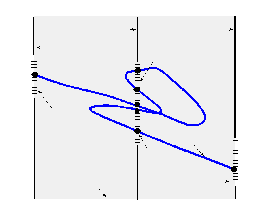
Since we are actually working with a 3-parameter family (1) of equations, this family defines implicitly a fibered space $\mathcal{S}\stackrel{{\scriptstyle p}}{{\to}}\mathcal{B}$ over the space of parameters $\mathcal{B}=\{(R,\nu,\mu)\}\subset{\mathbb{R}}^{3}$, where $\mathcal{S}$ is the total space of solutions of (1) and $\mathcal{B}$ forms the base of the fibered space. Moreover, the group $G$ acts on the total space of solutions $\mathcal{S}$. Therefore, we consider the quotient fibered space $\EuFrak{M}\stackrel{{\scriptstyle\pi}}{{\to}}\mathcal{B}$ modulo this action. Here $\EuFrak{M}=\mathcal{S}/\sim$ is the total moduli space, where $\sim$ is a relation between the points of $\mathcal{S}$ established by the group action which is compatible with $p$, that is, for any $s^{\prime},s\in\mathcal{S}$, $s^{\prime}\sim s$ if and only if $p(s^{\prime})=p(s)$ and there exists a $g\in G$ such that $s^{\prime}=g\!\cdot\!s$. Then $\pi$ is the map induced by $p$ after taking the quotient, and the points of $\EuFrak{M}$ are in one-to-one correspondence with $G$-orbits whose elements are all mapped by $p$ to the same point in the base $\mathcal{B}$. Thus, geometrically we have a fibered space, that is, a triple $(\EuFrak{M},\mathcal{B},\pi)$, depicted in Figure 1, whose fibers $\mathcal{M}_{\scriptscriptstyle{R,\nu,\mu}}=\pi^{-1}(R,\nu,\mu)$ over each point $(R,\nu,\mu)\in\mathcal{B}$ of the base are moduli spaces of solutions of the CGLE. Note that we do not know the explicit form of the map $\pi$. It is defined implicitly by equation (1). In essence, it is our goal to understand and reveal its properties. Therefore, the aim of the present study is to acquire a more global view of (a part of) the fibered space of $G$-orbits of the CGLE and its structure as we move around the point $(R,\nu,\mu)$ in the base space $\mathcal{B}$.

More precisely, and referring again to Figure 1, here we are interested in the (sub)fibered space $(\mathcal{I},\mathcal{B},\pi|\mathcal{I})\subset(\EuFrak{M},\mathcal{B},\pi)$, where the points of the subspace $\mathcal{I}\subset\EuFrak{M}$ are $G$-orbits of invariant solutions of the CGLE. Namely, these are solutions that satisfy, in addition to (1)–(2), the functional equation (4). Then the fiber of $\pi|\mathcal{I}$, $\mathcal{I}_{\scriptscriptstyle{R,\nu,\mu}}=(\pi|\mathcal{I})^{-1}(R,\nu,\mu)\subset\mathcal{M}_{\scriptscriptstyle{R,\nu,\mu}}$, over each point $(R,\nu,\mu)\in\mathcal{B}$ of the base is a moduli space of such invariant solutions of the CGLE. Note that a $G$-orbit in $\mathcal{I}_{\scriptscriptstyle{R,\nu,\mu}}$ is determined uniquely by a quadruple $\big(A(x,t,R,\nu,\mu),\varphi(R,\nu,\mu),S(R,\nu,\mu),T(R,\nu,\mu)\big)$, where $A(x,t,R,\nu,\mu)$ is an element of the orbit (that is, an invariant solution) over the point $(R,\nu,\mu)\in\mathcal{B}$. Further, for each point $(R,\nu,\mu)\in\mathcal{B}$ the space $\mathcal{I}_{\scriptscriptstyle{R,\nu,\mu}}$ is a union $\mathcal{I}_{\scriptscriptstyle{R,\nu,\mu}}=\bigcup_{\alpha}\Sigma_{\scriptscriptstyle{R,\nu,\mu}}^{(\alpha)}$ of symmetry classes $\Sigma_{\scriptscriptstyle{R,\nu,\mu}}^{(\alpha)}\subset\mathcal{I}_{\scriptscriptstyle{R,\nu,\mu}}$ of $G$-orbits. A number of such $G$-orbits and their symmetry classes were found in [23] at a particular point $(R_{\mathrm{o}},\nu_{\mathrm{o}},\mu_{\mathrm{o}})\in\mathcal{B}$. The main goal here is to understand structural changes in the spaces $\mathcal{I}_{\scriptscriptstyle{R,\nu,\mu}}$ as we trace paths in the fibered space $(\mathcal{I},\mathcal{B},\pi|\mathcal{I})$, starting from a set of $G$-orbits in the fiber $\mathcal{I}_{\scriptscriptstyle{R_{\mathrm{o}},\nu_{\mathrm{o}},\mu_{\mathrm{o}}}}$ and carrying them into another fiber $\mathcal{I}_{\scriptscriptstyle{R_{\mathrm{n}},\nu_{\mathrm{n}},\mu_{\mathrm{n}}}}$ over a point $(R_{\mathrm{n}},\nu_{\mathrm{n}},\mu_{\mathrm{n}})\neq(R_{\mathrm{o}},\nu_{\mathrm{o}},\mu_{\mathrm{o}})$ in the base $\mathcal{B}$ using a path following method [27].

Indeed, structural changes associated with additional symmetry breaking or gaining (vanishing and appearance of symmetry classes in $\mathcal{I}_{\scriptscriptstyle{R,\nu,\mu}}$) were frequently uncovered in the parameter regions traversed. This includes the identification of new symmetry classes (see, for example, the metamorphosis of the moduli space along the path $\mathcal{A}^{{\scriptscriptstyle({13})}}$ – Section 4.1 and Figure 9). Thus a complex and interesting structure of the fibered space $(\mathcal{I},\mathcal{B},\pi|\mathcal{I})$ was revealed. Sections 2 and 4 describe in detail the additional symmetries that are being gained or broken at particular values of the CGLE parameters. Such (abrupt) structural changes amount to a kind of “phase transition” in the moduli space, which is an interesting aspect to be considered as a focus for a subsequent detailed investigation.

To put all of the above in context, in contrast to studies which are concerned with continuation (deformation) of a single critical, singular or other non-generic point (with or without symmetry) of the space of solutions of (1) (for example, solutions which are stable, steady-states, or of the aforementioned traveling waves class) and their bifurcations, ours should be viewed as a study “in the large” of properties of the 3-dimensional family of moduli spaces $\mathcal{I}_{\scriptscriptstyle{R,\nu,\mu}}$ of invariant solutions within a certain general functional class, being approximated with a spectral-Galerkin discretization (the details of which appear in Section 3.1).

As we focus on solutions of the CGLE having the invariance (4), henceforth when we refer to $G$-orbits (of solutions of the CGLE) we mean $G$-orbits of invariant solutions of the CGLE which satisfy (4), unless otherwise indicated. We also note that during the continuation, most often the final parameter region of interest was sought by moving in the direction of varying values of $R$. However, at times we had to venture into a subdomain of the CGLE parameter space $\mathcal{B}$ by moving in a direction of varying $\nu$ and $\mu$ as well. Newton’s method, which is commonly used in path following methods [1, 19], is employed to solve an underdetermined system of nonlinear algebraic equations resulting from the discretization of the CGLE. To the best of our knowledge, the way in which the Newton step is computed here is new. The approach is conceptually simple, yet that is where its value lies: it led to the efficient computation of an accurate Newton step, making the solution of a computationally challenging problem with a large number (up to 32,260) of unknowns practical without the need of a cluster or supercomputer. These and other aspects of the numerical methodology are discussed in Section 3. We note here that the Newton step used is defined from the Moore-Penrose inverse [5]. This is one technique used in numerical continuation [1, 35], without the need to define phase, or gauge, conditions [19] to augment the underdetermined system. This offers an advantage since the best (or a suitable) choice of phase conditions may be problem dependent. The question of whether to impose phase conditions, or to simply work directly with the underdetermined system, thus arises. Here we chose to explore the latter approach. However, understanding the advantages that working with phase conditions may offer over the chosen approach is important and should be considered as a follow-up investigation.

As a bi-product of our study we note that, taking the presence of positive Lyapunov exponents for typical (that is, non-invariant) solutions as an indication of chaotic dynamics [28], both the initial and final parameter regions in our study exhibit chaotic behavior. Specifically, non-invariant solutions in the initial and final parameter region have, respectively, $5$ and $16$ positive Lyapunov exponents.¹¹ 1 Lyapunov exponents for typical (non-invariant) solutions were computed using the technique from [6]. This provides another motivation for conducting this study, which is to evaluate the potential benefits of using numerical continuation (on problems with a large number of unknowns) to continue multiple, distinct, unstable invariant solutions from one chaotic regime into another with the aim of ending, again, with multiple, distinct, unstable invariant solutions in the final region. One question that arises (see also [8]) is whether a significant number of the distinct solutions used as initial points to continue on will actually lead to solutions in distinct $G$-orbits in the final parameter region. While the possibility of this not happening cannot be ruled out, we found that options like alternating the choice of continuation parameter, or particular settings for tuning parameters in the numerical solvers, can increase the possibility of reaching a multitude of distinct $G$-orbits in the final desired parameter region.

A detailed account of the results obtained is provided in Section 4. We note here that the set of $G$-orbits in the fiber $\mathcal{I}_{\scriptscriptstyle{R_{\mathrm{o}},\nu_{\mathrm{o}},\mu_{\mathrm{o}}}}$ used as starting points in the path following method correspond to the first 15 $G$-orbits listed in the Appendix from [23]; these were selected simply to follow the order listed in said Appendix. The $G$-orbits from this initial set were carried from the point $(R_{\mathrm{o}},\nu_{\mathrm{o}},\mu_{\mathrm{o}})=(16,-7,5)$ in the CGLE parameter space to the point $(R_{\mathrm{n}},\nu_{\mathrm{n}},\mu_{\mathrm{n}})=(100,-7,5)$. The number of unknowns to solve for ranged between 4,000 and 32,260. Both the number of 15 $G$-orbits from [23] and the final point $(R_{\mathrm{n}},\nu_{\mathrm{n}},\mu_{\mathrm{n}})$ in the CGLE parameter space were chosen because we deemed them to be sufficient to help us gain insight into the symmetry changes occurring in the spaces $\mathcal{I}_{\scriptscriptstyle{R,\nu,\mu}}$ of the fibered space $(\mathcal{I},\mathcal{B},\pi|\mathcal{I})$, as well as to allow us to evaluate the potential for success of the proposed approach for computing multiple unstable invariant solutions in fixed parameter regions of a dynamical system which exhibits chaotic behavior.

The initial set of $G$-orbits led to distinct, new $G$-orbits of invariant solutions of the CGLE along the continuation paths and in the final parameter region. The solutions in the resulting $G$-orbits are unstable, and have multiple modes and frequencies active in their spatial and temporal spectra, respectively. The fact that the computed solutions are unstable suggests that they may belong to the set of (infinitely many) unstable periodic orbits embedded in chaotic attractors [9, 20, 8]. This direction, by itself, is certainly very interesting to pursue in a future study of the dynamics of the CGLE.

To conclude the introduction we note that previous numerical continuation studies of the CGLE include [32], where bifurcations from a stable rotating wave to two-tori (of the generalized traveling wave class) were identified. Values of $L_{\scriptscriptstyle x}=1$ and $R\leq 180$ in the formulation (1)–(2) were considered, giving $L\approx 13.42$ for the maximum length of the spatial period in the formulation (3). In comparison, the values $L_{\scriptscriptstyle x}=2\pi$ and $R\leq 100$ in our study yield a maximum value of $L\approx 62.83$ in (3). The values of $\nu$ and $\mu$ used in [32] are different from those in the current study, but in both cases they belong to the Benjamin-Feir unstable region $1+\mu\nu<0$ [34]. A different study [7] considers traveling waves solutions, where the CGLE reduces to a system of three coupled ordinary differential equations (ODEs). Continuation was performed on the system of three ODEs for different values of $L$ up to $512$ and various chaotic regions were classified.

Other studies can be found in [26], where transition to chaos from a limit cycle of the CGLE is investigated, [18], in which the bifurcation structure and dynamics of even solutions of the CGLE are analyzed, and [22], which studies the dynamics of the CGLE in heteroclinic cycles, focused on invariant ${\mathbb{Z}}_{2}$-subspaces. A numerical study on solutions fixed by the ${\mathbb{Z}}_{2}$-symmetry of the CGLE and their stability with respect to symmetry-breaking perturbations appears in [3], where values of $R=1.05,16,36$ are considered, and a spatial period of $L_{\scriptscriptstyle x}=2\pi$ was used (the latter being the same as in the current study). The subsequent study [4] considers symmetry-breaking perturbations for solutions fixed by the spatial translation symmetry, for (discrete) values of the parameter $R$ in the range $[4.2,80]$.

The CGLE has a number of well known symmetries that are central to its behavior [2]. In particular, equations (1)–(2) have a three-parameter group

$$G={\mathbb{T}}^{2}\times{\mathbb{R}}$$

(5)

of continuous symmetries generated by space-time translations $x\rightarrow x+\sigma$, $t\rightarrow t+\tau$ and a rotation $A\rightarrow\mathrm{e}^{\mathrm{i}\theta}A$ of the complex field $A(x,t)$, in addition to being invariant under the action of the discrete group of transformations $A(x,t)\rightarrow A(-x,t)$ of spatial reflections. In other words, if $A(x,t)$ is a solution of equations (1)–(2), then so are

	$\displaystyle\mathrm{e}^{\mathrm{i}\theta}A(x,t)$	,		(6)
	$\displaystyle A(x+\sigma,t)$	,		(7)
	$\displaystyle A(x,t+\tau)$	,		(8)
	$\displaystyle A(-x,t)$	,		(9)

for any $(\theta,\sigma,\tau)\in G$. In the present study it is the group $G$ generated by the continuous symmetries (6)–(8) which (explicitly) enters the problem formulation. Namely, for a given solution $A(x,t)$ of the CGLE, let us consider the isotropy subgroup $G_{\!{\scriptscriptstyle{{A}}}}$ of $G$ at $A$,

$$G_{\!{\scriptscriptstyle{{A}}}}=\{(\varphi,S,T)\in G\ \,|\ \,A(x,t)=\mathrm{e}^{\mathrm{i}\varphi}A(x+S,t+T)\},$$

(10)

which consists of elements of the symmetry group $G={\mathbb{T}}^{2}\times{\mathbb{R}}$ leaving $A$ invariant. With that in mind, we pose the problem: seek solutions $A(x,t)$ of the CGLE satisfying

$$A(x,t)=\mathrm{e}^{\mathrm{i}\varphi}A(x+S,t+T),$$

(11)

for $(\varphi,S,T)\in G$ also unknown and to be determined. In other words, find orbits $G\cdot A$ of $G$ generated by solutions $A$ of the CGLE which are invariant under the action of some subgroup $G_{\!{\scriptscriptstyle{{A}}}}\subset G$, that is, $G_{\!{\scriptscriptstyle{{A}}}}\cdot A=A$. Here, at least one subgroup of $G_{\!{\scriptscriptstyle{{A}}}}$ generated by an element $(\varphi,S,T)\in G$ is also to be determined.

As is clear from (11), the case $\varphi=S=0$, $T>0$, would result in a time-periodic solution. Within the more general context of the problem of seeking solutions of a dynamical system fixed by the action of a subgroup of the system’s symmetry group (which also contains time translation), as is the case resulting from $T>0$ and nonzero $\varphi$ or $S$ in (11), such invariant solutions are also referred to as relative time-periodic solutions. Since the solutions sought must satisfy the boundary (space-periodicity) condition (2), it is easy to see that if $S=L_{\scriptscriptstyle x}/q$ for some integer $q>1$, then $|A(x,t)|=|A(x,t+qT)|$, whereas if both $S=L_{\scriptscriptstyle x}/q$ and $\varphi=2\pi/q$ for some integer $q>1$, then $A(x,t)=A(x,t+qT)$ and, therefore, $(0,0,qT)\in G_{\!{\scriptscriptstyle{{A}}}}$ (i.e., $A$ is time-periodic, with time period $qT$).

Notice that if $(\varphi,S,T)\in G_{\!{\scriptscriptstyle{{A}}}}$, the triples $(j\varphi,jS,jT),\ j\in{\mathbb{Z}},$ are also elements of the isotropy subgroup $G_{\!{\scriptscriptstyle{{A}}}}$. Hence, $(\varphi,S,T)$ generates a subgroup of $G_{\!{\scriptscriptstyle{{A}}}}$. Thus, the problem that we aim to solve numerically can be described succinctly as follows:

1. 1.

   Given a point ${p}_{{\scriptscriptstyle{{0}}}}=({R}_{{\scriptscriptstyle{{0}}}},{\nu}_{{\scriptscriptstyle{{0}}}},{\mu}_{{\scriptscriptstyle{{0}}}})$ in the parameter space of the CGLE, find a solution $A_{\!{\scriptscriptstyle{p}_{{\scriptscriptstyle{{0}}}}}}(x,t)$ of the CGLE and a generator $(\varphi({p}_{{\scriptscriptstyle{{0}}}}),S({p}_{{\scriptscriptstyle{{0}}}}),T({p}_{{\scriptscriptstyle{{0}}}}))$ of a subgroup of the isotropy subgroup $G_{\!{\scriptscriptstyle{{A_{p_{\scriptscriptstyle 0}}}}}}$, such that condition (11) holds. That is, $A_{\!{\scriptscriptstyle{p}_{{\scriptscriptstyle{{0}}}}}}$ is an invariant solution of the CGLE under the action of the subgroup of $G_{\!{\scriptscriptstyle{{A_{p_{\scriptscriptstyle 0}}}}}}$ generated by $(\varphi({p}_{{\scriptscriptstyle{{0}}}}),S({p}_{{\scriptscriptstyle{{0}}}}),T({p}_{{\scriptscriptstyle{{0}}}}))$.

2. 2.

   Then, starting from ${p}_{{\scriptscriptstyle{{0}}}}=({R}_{{\scriptscriptstyle{{0}}}},{\nu}_{{\scriptscriptstyle{{0}}}},{\mu}_{{\scriptscriptstyle{{0}}}})$, vary the point $p=(R,\nu,\mu)$ along a subspace in the parameter space of the CGLE, ending at a point ${p}_{{\scriptscriptstyle{{\mathrm{N}}}}}=({R}_{{\scriptscriptstyle{{\mathrm{N}}}}},{\nu}_{{\scriptscriptstyle{{\mathrm{N}}}}},{\mu}_{{\scriptscriptstyle{{\mathrm{N}}}}})$, to find a sequence of new invariant solutions $A_{\!{\scriptscriptstyle p}}(x,t)$ and generators $(\varphi(p),S(p),T(p))$ of subgroups of their corresponding isotropy subgroups $G_{\!{\scriptscriptstyle{{A_{p}}}}}$.

In reference [23] we found 77 distinct unstable invariant solutions (that is, 77 $G$-orbits generated by distinct invariant solutions) of the CGLE at the point ${p}_{{\scriptscriptstyle{{0}}}}=({R}_{{\scriptscriptstyle{{0}}}},{\nu}_{{\scriptscriptstyle{{0}}}},{\mu}_{{\scriptscriptstyle{{0}}}})=(16,-7,5)$ of the parameter space of the CGLE, thus addressing the first part of the problem. Here, we take the first 15 of these solutions, per the listing from the Appendix in [23], and address the second part of the problem. Specifically, using numerical continuation (as described in Section 3) we found 15 sequences (or discrete continuation paths)

$$\begin{split}\mathcal{A}^{{\scriptscriptstyle({i})}}=\{A_{\!{\scriptscriptstyle{p}_{{\scriptscriptstyle{{k}}}}^{{\scriptscriptstyle{{(i)}}}}}}&(x,t)\,;\,(\varphi({p}_{{\scriptscriptstyle{{k}}}}^{{\scriptscriptstyle{{(i)}}}}),S({p}_{{\scriptscriptstyle{{k}}}}^{{\scriptscriptstyle{{(i)}}}}),T({p}_{{\scriptscriptstyle{{k}}}}^{{\scriptscriptstyle{{(i)}}}}))\ \,|\ \,\\ {p}_{{\scriptscriptstyle{{k}}}}^{{\scriptscriptstyle{{(i)}}}}&=({R}_{{\scriptscriptstyle{{k}}}}^{{\scriptscriptstyle{{(i)}}}},{\nu}_{{\scriptscriptstyle{{k}}}}^{{\scriptscriptstyle{{(i)}}}},{\mu}_{{\scriptscriptstyle{{k}}}}^{{\scriptscriptstyle{{(i)}}}})\in[9,100]\times[-7,-2.7]\times[-0.05,5.98],\ \ 0\leq k\leq\mathrm{N}^{\scriptscriptstyle(i)}\},\end{split}$$

(12)

$i=1,\ldots,15$, of new invariant solutions (11) of the CGLE and corresponding generators of subgroups of their isotropy subgroups $G_{\!{\scriptscriptstyle{{A_{\!{\scriptscriptstyle{p}_{{\scriptscriptstyle{{k}}}}^{{\scriptscriptstyle{{(i)}}}}}}}}}}$. In (12), the number $\mathrm{N}^{\scriptscriptstyle(i)}$ of invariant solutions in a sequence is at least 100 and, for each $i=1,\ldots,15$, the final point ${p}_{{\scriptscriptstyle{{\mathrm{N}^{\scriptscriptstyle(i)}}}}}^{{\scriptscriptstyle{{(i)}}}}$ in the CGLE parameter space was fixed at ${p}_{{\scriptscriptstyle{{\mathrm{N}^{\scriptscriptstyle(i)}}}}}^{{\scriptscriptstyle{{(i)}}}}=({R}_{{\scriptscriptstyle{{\mathrm{N}^{\scriptscriptstyle(i)}}}}}^{{\scriptscriptstyle{{(i)}}}},{\nu}_{{\scriptscriptstyle{{\mathrm{N}^{\scriptscriptstyle(i)}}}}}^{{\scriptscriptstyle{{(i)}}}},{\mu}_{{\scriptscriptstyle{{\mathrm{N}^{\scriptscriptstyle(i)}}}}}^{{\scriptscriptstyle{{(i)}}}})=(100,-7,5)$. Thus, the sequences (12) can be thought of as a deformation of an initial set of distinct $G$-orbits at ${p}_{{\scriptscriptstyle{{0}}}}=(16,-7,5)$ into a final set of $G$-orbits at ${p}_{{\scriptscriptstyle{{\mathrm{N}}}}}=(100,-7,5)$, which in this study are also distinct with the only exception being that the final orbits in the sequences $\mathcal{A}^{{\scriptscriptstyle({2})}}$ and $\mathcal{A}^{{\scriptscriptstyle({4})}}$ at ${p}_{{\scriptscriptstyle{{\mathrm{N}}}}}$ happened to coincide (details are provided in Section 4). In other words, if we think of the space of $G$-orbits as fibered over the parameter space $\mathcal{B}$ of the CGLE (the base of the fibered space), then the sequences (or continuation paths) $\mathcal{A}^{{\scriptscriptstyle({i})}}$ can be thought of as (discrete) sections of the fibered space $(\mathcal{I},\mathcal{B},\pi|\mathcal{I})$. Interestingly, several of the sequences $\mathcal{A}^{{\scriptscriptstyle({i})}}$ that we have computed contain solutions with additional symmetries (which we describe in detail later in this section), thus revealing an intricate structure of the fibered space $(\mathcal{I},\mathcal{B},\pi|\mathcal{I})$.

Note that the meaning of the space-periodicity boundary condition (2) is that any solution $A(x,t)$ in the class of solutions of the CGLE that we seek has a subgroup in its isotropy subgroup $G_{\!{\scriptscriptstyle{{A}}}}$ which is generated by $(0,L_{\scriptscriptstyle x},0)$. In other words we restrict, a priori, the class of solutions of the CGLE that we look for to the one that contains, at a minimum, solutions with symmetry (2). This allows us to represent $A(x,t)$ as a Fourier series

$$A(x,t)=\sum_{m\in{\mathbb{Z}}}a_{\scriptscriptstyle{{m}}}(t)\mathrm{e}^{\mathrm{i}k_{\scriptscriptstyle m}x},$$

(13)

where $k_{\scriptscriptstyle m}=2\pi m/L_{\scriptscriptstyle x}$ denotes the $m$-th wavenumber in the expansion. From the group-invariance condition (11) it then follows that the complex-valued Fourier coefficient functions $a_{\scriptscriptstyle{{m}}}(t)$ in (13) satisfy

$$a_{\scriptscriptstyle{{m}}}(t)=\mathrm{e}^{\mathrm{i}\varphi}\mathrm{e}^{\mathrm{i}k_{\scriptscriptstyle m}S}a_{\scriptscriptstyle{{m}}}(t+T)$$

(14)

for all $m\in{\mathbb{Z}}$. Because of the presence of symmetry (2), the solutions sought can be restricted to those with elements $(\varphi,S,T)\in G$ having $S\in[0,L_{\scriptscriptstyle x})$.

Moreover, since the CGLE is invariant under the action of the group ${\mathbb{Z}}_{2}$ of spatial reflections $A(x,t)\rightarrow A(-x,t)$, to any solution $A(x,t)$ of the CGLE having $(0,L_{\scriptscriptstyle x},0)$ and $(\varphi,S,T)$ as generators of subgroups of the isotropy subgroup $G_{\!{\scriptscriptstyle{{A}}}}$ (defined in (10)) there corresponds a solution $\tilde{A}(x,t):=A(-x,t)$ having $(0,L_{\scriptscriptstyle x},0)$ and $(\varphi,L_{\scriptscriptstyle x}\!-\!S,T)$ as generators of subgroups of the isotropy subgroup $G_{\!{\scriptscriptstyle{{\tilde{A}}}}}$. This can be seen from the chain of equalities

	$\displaystyle\tilde{A}(x,t)\ :=\ A(-x,t)$	$\displaystyle=$	$\displaystyle\mathrm{e}^{\mathrm{i}\varphi}A(-x+S,t+T)\hskip 32.50005pt\mbox{by (\ref{eqn:cgle_invariant_solution})}$		(15)
		$\displaystyle=$	$\displaystyle\mathrm{e}^{\mathrm{i}\varphi}\tilde{A}(x-S,t+T)\hskip 40.00006pt\mbox{by definition of $\tilde{A}$}$
		$\displaystyle=$	$\displaystyle\mathrm{e}^{\mathrm{i}\varphi}\tilde{A}(x+(L_{\scriptscriptstyle x}-S),t+T)\quad\mbox{by (\ref{eqn:cgle_bcs}).}$

To express the above in a more symmetric form, let us introduce $\delta=|L_{\scriptscriptstyle x}/2-S|$. Then, if $A(x,t)$ is a solution of the CGLE having $(0,L_{\scriptscriptstyle x},0)$ and $(\varphi,L_{\scriptscriptstyle x}/2\pm\delta,T)$ as generators of subgroups of the isotropy subgroup $G_{\!{\scriptscriptstyle{{A}}}}$, the solution $\tilde{A}(x,t):=A(-x,t)$ has $(0,L_{\scriptscriptstyle x},0)$ and $(\varphi,L_{\scriptscriptstyle x}/2\mp\delta,T)$ as generators of subgroups of the isotropy subgroup $G_{\!{\scriptscriptstyle{{\tilde{A}}}}}$. We shall call the invariant solutions $(A;\varphi,L_{\scriptscriptstyle x}/2\pm\delta,T)$ and $(\tilde{A};\varphi,L_{\scriptscriptstyle x}/2\mp\delta,T)$, as well as their corresponding orbits $G\cdot A$ and $G\cdot\tilde{A}$, conjugate to each other under the (involutive) action of the group ${\mathbb{Z}}_{2}$ of spatial reflection symmetry of the CGLE.

Now, while invariance of solutions of the CGLE other than that defined by (11) and (2) is not part of the problem formulation (10)–(11), it is clearly not excluded from it. The CGLE may admit solutions having symmetries other than (or in addition to) that defined by (11) and several of the solutions resulting from our study do have additional symmetries. In what follows we discuss some such symmetries and their properties. We emphasize that our treatment on additional types of symmetries exhibited by solutions of the CGLE is not exhaustive, but rather inclusive of material relevant to the discussion on our results in Section 4.

For instance, there may exist solutions of the CGLE satisfying

	$\displaystyle A(x,t)$	$\displaystyle=$	$\displaystyle\mathrm{e}^{\mathrm{i}2\pi/l}A(x+L_{\scriptscriptstyle x}/l,t),\hskip 22.50003pt\mbox{for some $l\in{\mathbb{N}}$, $l>1$,}$		(16)
	$\displaystyle A(x,t)$	$\displaystyle=$	$\displaystyle\hskip 10.00002ptA(-x+2c_{\scriptscriptstyle{1}},t)\hskip 37.50005pt\mbox{for some $c_{\scriptscriptstyle{1}}\in{\mathbb{R}}$,}$		(17)
	$\displaystyle A(x,t)$	$\displaystyle=$	$\displaystyle-A(-x+2c_{\scriptscriptstyle{2}},t)\hskip 40.00006pt\mbox{for some $c_{\scriptscriptstyle{2}}\in{\mathbb{R}}$.}$		(18)

Note that (16) describes solutions fixed by a composition of the actions (7) and (6), and gives $(2\pi/l,L_{\scriptscriptstyle x}/l,0)$ as one generator of a subgroup of $G_{\!{\scriptscriptstyle{{A}}}}$. From (16) it is also clear that the absolute value of such a solution has spatial period of $L_{\scriptscriptstyle x}/l$. Furthermore, by substituting condition (16) into the Fourier series expansion (13) it follows that the Fourier coefficient functions $a_{\scriptscriptstyle{{m}}}(t)$ of a solution with symmetry (16) satisfy

$$a_{\scriptscriptstyle{{m}}}(t)=\left\{\begin{array}[]{ll}\mbox{nonzero}&\mbox{if $m\in\{l\tilde{m}-1,\ \tilde{m}\in{\mathbb{Z}}\}$}\\ 0&\mbox{otherwise}.\end{array}\right.$$

(19)

Symmetries (17) and (18) describe solutions that are, respectively, even about $x=c_{\scriptscriptstyle{1}}$ or odd about $x=c_{\scriptscriptstyle{2}}$ for some real numbers $c_{\scriptscriptstyle{1}},c_{\scriptscriptstyle{2}}$. (These solutions are fixed by a composition of the actions (9), (7), and (6).) From (17) and the periodic boundary condition (2) it follows that a solution even about $x=c_{\scriptscriptstyle{1}}$ is also even about $x=c_{\scriptscriptstyle{1}}+L_{\scriptscriptstyle x}/2$; similarly a solution odd about $x=c_{\scriptscriptstyle{2}}$ is also odd about $x=c_{\scriptscriptstyle{2}}+L_{\scriptscriptstyle x}/2$. The Fourier coefficient functions $a_{\scriptscriptstyle{{m}}}(t)$ in (13) of a solution even about $x=c_{\scriptscriptstyle{1}}$ satisfy

$$a_{\scriptscriptstyle{{-m}}}(t)=a_{\scriptscriptstyle{{m}}}(t)\,\mathrm{e}^{\mathrm{i}k_{\scriptscriptstyle m}2c_{\scriptscriptstyle{1}}}\ ,\ \ m=0,1,2,\ldots\,,$$

(20)

whereas for a solution odd about $x=c_{\scriptscriptstyle{2}}$ one has

$$a_{\scriptscriptstyle{{-m}}}(t)=-a_{\scriptscriptstyle{{m}}}(t)\,\mathrm{e}^{\mathrm{i}k_{\scriptscriptstyle m}2c_{\scriptscriptstyle{2}}}\\ ,\ \ m=0,1,2,\ldots\,.$$

(21)

From (19), (20), and (21) it follows that restricting the search for solutions to those possessing symmetries (16), (17), or (18) would lead to a reduction in the number of unknowns. However, as already mentioned, we did not make a priori such a restriction in order to allow for a more general set of solutions. Finally, we point out that a solution having both symmetries (16) and (17) also satisfies

$$A(-x+2(c_{\scriptscriptstyle{1}}+L_{\scriptscriptstyle x}/(2l)),t)=\mathrm{e}^{\mathrm{i}2\pi/l}A(x,t)\,.$$

(22)

In particular, note that a solution satisfying (16) for $l=2$ and which is even about $x=c_{\scriptscriptstyle{1}}$ is also odd about $x=c_{\scriptscriptstyle{2}}=c_{\scriptscriptstyle{1}}+L_{\scriptscriptstyle x}/4$.

For a solution satisfying (11) and (16) it follows that $(\varphi-2\pi/l,S-L_{\scriptscriptstyle x}/l,T)$ is another generator of a subgroup of $G_{\!{\scriptscriptstyle{{A}}}}$. In particular, if it happens that for such a solution one has $S=L_{\scriptscriptstyle x}/l$, then $|A(x,t)|=|A(x,t+T)|$ is satisfied, whereas if both $S=L_{\scriptscriptstyle x}/l$ and $\varphi=2\pi/l$, then $A(x,t)=A(x,t+T)$ also holds. As for invariant solutions (11) that also possess symmetry (17), note that, for each $m=0,1,2,\ldots$,

	$\displaystyle a_{\scriptscriptstyle{{-m}}}(t)$	$\displaystyle=$	$\displaystyle\mathrm{e}^{\mathrm{i}\varphi}\mathrm{e}^{-\mathrm{i}k_{\scriptscriptstyle m}S}a_{\scriptscriptstyle{{-m}}}(t+T)\hskip 40.00006pt\mbox{by (\ref{eqn:am_invariant})}$		(23)
		$\displaystyle=$	$\displaystyle\mathrm{e}^{\mathrm{i}\varphi}\mathrm{e}^{-\mathrm{i}k_{\scriptscriptstyle m}S}a_{\scriptscriptstyle{{m}}}(t+T)\,\mathrm{e}^{\mathrm{i}k_{\scriptscriptstyle m}2c_{\scriptscriptstyle{1}}}\hskip 15.00002pt\mbox{by (\ref{eqn:Fcoefs_even}).}$

On the other hand, for each $m=0,1,2,\ldots$,

	$\displaystyle a_{\scriptscriptstyle{{-m}}}(t)$	$\displaystyle=$	$\displaystyle a_{\scriptscriptstyle{{m}}}(t)\,\mathrm{e}^{\mathrm{i}k_{\scriptscriptstyle m}2c_{\scriptscriptstyle{1}}}\hskip 70.0001pt\mbox{by (\ref{eqn:Fcoefs_even})}$		(24)
		$\displaystyle=$	$\displaystyle\mathrm{e}^{\mathrm{i}\varphi}\mathrm{e}^{\mathrm{i}k_{\scriptscriptstyle m}S}a_{\scriptscriptstyle{{m}}}(t+T)\,\mathrm{e}^{\mathrm{i}k_{\scriptscriptstyle m}2c_{\scriptscriptstyle{1}}}\hskip 15.00002pt\mbox{by (\ref{eqn:am_invariant}).}$

From (23) and (24) it follows that we must have $\mathrm{e}^{-\mathrm{i}k_{\scriptscriptstyle m}S}\ =\ \mathrm{e}^{\mathrm{i}k_{\scriptscriptstyle m}S}$ for all $m\in{\mathbb{Z}}$, which holds whenever $S$ is an integer multiple of $L_{\scriptscriptstyle x}/2$ (recall that $k_{\scriptscriptstyle m}=2\pi m/L_{\scriptscriptstyle x}$). The case for invariant solutions (11) with the additional symmetry (18) is analogous. Therefore, solutions satisfying (11) which also posses symmetries (17) or (18) exist in subspaces of the solution space $(A;\varphi,S,T)$ for which either $S=0$ or $S=L_{\scriptscriptstyle x}/2$ (since, by the periodic boundary conditions (2), $S$ can be restricted to be in the interval $[0,L_{\scriptscriptstyle x})$).

To illustrate some of the aforementioned symmetries of solutions of the CGLE, Figures 2–3 display several plots that aid in visualizing the invariant properties. Figure 2 shows a solution of the CGLE having symmetry (11), but none of (16)–(18). This solution belongs to the sequence $\mathcal{A}^{{\scriptscriptstyle({5})}}$ (see (12)) resulting from the numerical continuation procedure to be described in Section 3, that is, from the continuation path for the sequence listed with id 5 in Tables 1–2 (refer to Section 4). The time evolution, represented as curves on the plane with coordinates defined by the real part $\Re(A)$ and imaginary part $\Im(A)$ of the solution $A(x,t)$ at different times within the interval $[0,T]$, is depicted in Figures 2a–2d. The excitation of multiple temporal frequencies is apparent from these curves. For single-frequency solutions $A(x,t)=B(x)\mathrm{e}^{\mathrm{i}\omega t}$ or generalized traveling waves $A(x,t)=\rho(x-vt)\mathrm{e}^{\mathrm{i}\phi(x-vt)}\mathrm{e}^{\mathrm{i}\omega t}$ (where $\omega$ is some single frequency), plots of this kind would show, except for a rotation, the same curve at each point in time. Therefore it is clear that the solution depicted in Figures 2a–2d is not of either of these single-frequency types. Note also that the curve at time $t=T$ differs only by a rotation from that at time $t=0$ due to the rotation of the complex field $A(x,0)\rightarrow\mathrm{e}^{\mathrm{i}\varphi}A(x+S,T)$. Repeated patterns resulting from invariance due to time periodicity and the nonzero space translation $S$ is better observed from surface plots of the absolute value $|A|$ of $A(x,t)$ over several space and time periods, as in Figure 2e.

A solution possessing all of the symmetries (16)–(18), in addition to the symmetry (11), is shown in Figure 3. The plots represent a solution which belongs to the sequence of solutions under id 15 in Tables 1–3 (refer to Section 4), computed at the point $(R,\nu,\mu)=(100,-7,5)$ of the CGLE parameter space. Surface plots of the real part $\Re(A)$, imaginary part $\Im(A)$, and absolute value $|A|$ of the solution $A(x,t)$ are shown in Figures 3a–3c, where $(x,t)\in[0,2L_{\scriptscriptstyle x}]\times[0,2T]$, that is, the surfaces are plotted over two space and two time periods. For this solution, symmetry (16) holds with $l=2$. Since, in addition, the solution is even about $x=\tilde{m}L_{\scriptscriptstyle x}/4$, for $\tilde{m}\in{\mathbb{Z}}$ odd, it follows from (22) that the solution is also odd about $x=(\tilde{m}+1)L_{\scriptscriptstyle x}/4$. Finally, the absolute value of the solution has spatial period $L_{\scriptscriptstyle x}/2$ and is time-periodic, with period $T$. As seen in Figures 3a–3d, pattern similarities in both space and time are easily observed in the presence of the additional symmetries (16)–(18).

We conclude this section by noting the following fact. Suppose that for some $(\tilde{\varphi},c,\tilde{T})\in G$, where $G$ is the group of continuous symmetries of the CGLE (refer to (5)), a solution $A(x,t)$ of the CGLE has the symmetry

$$A(x,t)=\mathrm{e}^{\mathrm{i}\tilde{\varphi}}A(-x+c,t+\tilde{T}).$$

(25)

The Fourier coefficient functions $a_{\scriptscriptstyle{{m}}}(t)$ in (13) of such a solution satisfy

$$a_{\scriptscriptstyle{{-m}}}(t)=a_{\scriptscriptstyle{{m}}}(t+\tilde{T})\,\mathrm{e}^{\mathrm{i}\tilde{\varphi}}\mathrm{e}^{\mathrm{i}k_{\scriptscriptstyle m}c}\ ,\ \ m=0,1,2,\ldots\,.$$

(26)

The right-hand side of (25) is the result of the (left) action on $A(x,t)$ of the composition $(\tilde{\varphi},c,\tilde{T})\circ(x\rightarrow-x)$, and after a (left) action of said composition on both sides of (25) one obtains that

	$\displaystyle A(x,t)$	$\displaystyle=$	$\displaystyle\mathrm{e}^{\mathrm{i}\tilde{\varphi}}A(-x+c,t+\tilde{T})$		(27)
		$\displaystyle=$	$\displaystyle\mathrm{e}^{\mathrm{i}2\tilde{\varphi}}A(x,t+2\tilde{T}).$

Hence $(2\tilde{\varphi},0,2\tilde{T})\in G_{\!{\scriptscriptstyle{{A}}}}$, where $G_{\!{\scriptscriptstyle{{A}}}}$ is the isotropy subgroup defined in (10). Also, note that we have

$$[(\tilde{\varphi},c,\tilde{T})\circ(x\rightarrow-x)]^{2}\ =\ (2\tilde{\varphi},0,2\tilde{T})\ \in\ G,$$

for any element $(\tilde{\varphi},c,\tilde{T})$ in the group $G$ of continuous symmetries of the CGLE. Conversely, let $(\tilde{\varphi},0,\tilde{T})\in G_{\!{\scriptscriptstyle{{A}}}}$ for some solution $A(x,t)$ of the CGLE. Then we have

$$[(\tilde{\varphi}/2+k\pi,\,c\,,\tilde{T}/2)\circ(x\rightarrow-x)]^{2}\ =\ (\tilde{\varphi},0,\tilde{T})$$

for every $k\in{\mathbb{Z}}$ and $c\in{\mathbb{R}}$. Therefore, solutions of the CGLE with symmetry (25) do possess symmetry (11) of the type we seek, and, conversely, a solution with symmetry (11) may also possess the additional symmetry (25). An example of solutions having both symmetries (11) and (25) is described in Section 4 (cf. Figure 9). Such solutions appeared in the continuation path for the sequence listed with id 13 in Tables 1–3 (refer to Section 4), that is, in the sequence $\mathcal{A}^{{\scriptscriptstyle({13})}}$ (see (12)).

Finally, note that if a solution $A(x,t)$ of the CGLE having symmetry (11) for $S=0$ or $S=L_{\scriptscriptstyle x}/2$ also satisfies

$$A(x,t)=\mathrm{e}^{\mathrm{i}\hat{\varphi}}A(-x+\hat{c},t)$$

(28)

for some real numbers $\hat{\varphi}$ and $\hat{c}$ (an example being solutions with the additional symmetry (17), where $\hat{\varphi}$ = 0, or with the additional symmetry (18), for which $\hat{\varphi}=\pi$), then

$$A(x,t)\ =\ \mathrm{e}^{\mathrm{i}(\hat{\varphi}+2\varphi)}A(-x+\hat{c},t+2T).$$

That is, such solution $A$ also has symmetry (25). Therefore, one should expect to find solutions having both symmetries (11) and (25) in subspaces of the space of solutions $(A;\varphi,S,T)$ for which either $S=0$, by (27), or $S\in\{0,L_{\scriptscriptstyle x}/2\}$, if symmetry (28) is also present.

As noted in Section 1, having computed previously in [23] a set of unstable invariant solutions of the CGLE for fixed values of the parameters $(R,\nu,\mu)$, our first goal is to employ numerical continuation to carry solutions of this initial set into solutions in a regime with a different set of parameter values $(R,\nu,\mu)$. To achieve this, we discretize using Fourier series expansions in both space and time to derive an underdetermined system of nonlinear algebraic equations from which invariant solutions of the CGLE are sought. This discretization was used in the previous study [23]. The associated material which is directly relevant to the current study is summarized in Sections 3.1 and 3.2 below in order to make the present account self-contained. Details concerning the numerical continuation, which was not a component of the previous study [23], are provided in Section 3.3.

References

- [1] Eugene L. Allgower and Kurt Georg. Introduction to Numerical Continuation Methods. Classics in Applied Mathematics. SIAM, 2003.
- [2] Igor S. Aranson and Lorenz Kramer. The world of the complex Ginzburg-Landau equation. Rev. Mod. Phys., 74:99–143, 2002.
- [3] Philip J. Aston and Carlo R. Laing. Symmetry and chaos in the complex Ginzburg-Landau equation. I. Reflectional symmetries. Dynam. Stability Systems, 14:233–253, 1999.
- [4] Philip J. Aston and Carlo R. Laing. Symmetry and chaos in the complex Ginzburg-Landau equation. II. Translational symmetries. Physica D, 135:79–97, 2000.
- [5] Adi Ben-Israel and Thomas N.E. Greville. Generalized Inverses : Theory and Applications. Springer-Verlag, 2003.
- [6] G. Benettin, L. Galgani, A. Giorgilli, and J.-M. Strelcyn. Lyapunov characteristic exponents for smooth dynamical systems and for Hamiltonian systems; A method for computing all of them. Part I: Theory. Meccanica, 15:9–20, 1980.
- [7] Lutz Brusch, Alessandro Torcini, Martin van Hecke, Martín G. Zimmermann, and Markus Bär. Modulated amplitude waves and defect formation in the one-dimensional complex Ginzburg-Landau equation. Physica D, 160:127–148, 2001.
- [8] Gary J. Chandler and Rich R. Kerswell. Invariant recurrent solutions embedded in a turbulent two-dimensional Kolmogorov flow. J. Fluid Mech., 722:554–595, 2013.
- [9] P. Cvitanović, R. Artuso, P. Dahlqvist, R. Mainieri, G. Tanner, G. Vattay, N. Whelan, and A. Wirzba. Chaos: Classical and Quantum. 2014. Webbook available at chaosbook.org.
- [10] Arjen Doelman. Slow time-periodic solutions of the Ginzburg-Landau equation. Physica D, 40:156–172, 1989.
- [11] Arjen Doelman and Edriss S. Titi. Regularity of solutions and the convergence of the Galerkin method in the Ginzburg-Landau equation. Numer. Funct. Anal. Optim., 14(3-4):299–321, 1993.
- [12] M. Frigo and S. G. Johnson. FFTW: An adaptive software architecture for the FFT. In ICASSP Conference Proceedings, volume 3, pages 1381–1384, 1998. http://www.fftw.org/.
- [13] Gene H. Golub and Charles F. Van Loan. Matrix Computations. The Johns Hopkins University Press, 1996.
- [14] Anne Greenbaum. Iterative Methods for Solving Linear Systems. Frontiers in Applied Mathematics. SIAM, 1997.
- [15] Philip Holmes. Spatial structure of time-periodic solutions of the Ginzburg-Landau equation. Physica D, 23:84–90, 1986.
- [16] M. S. Jolly, R. Temam, and C. Xiong. Convergence of a chaotic attractor with increased spatial resolution of the Ginzburg-Landau equation. Chaos Solitons Fractals, 5(10):1833–1845, 1995.
- [17] Todd Kapitula and Stanislaus Maier-Paape. Spatial dynamics of time-periodic solutions for the Ginzburg-Landau equation. Zeitschrift für Angewandte Mathematik und Physik, 47:265–305, 1996.
- [18] Laurence R. Keefe. Dynamics of perturbed wavetrain solutions to the Ginzburg-Landau equation. Stud. Appl. Math., 73(2):91–153, 1985.
- [19] Y. A. Kuznetsov. Elements of Applied Bifurcation Theory. Springer-Verlag, 1998.
- [20] Y. Lan. Cycle expansions: From maps to turbulence. Commun Nonlinear Sci Numer Simulat, 15:502–526, 2010.
- [21] C. David Levermore and Marcel Oliver. The complex Ginzburg-Landau equation as a model problem. In Dynamical Systems and Probabilistic Methods in Partial Differential Equations, volume 31 of Lectures in Appl. Math., pages 141–190. Amer. Math. Soc., Providence, RI, 1996.
- [22] D. J. B. Lloyd, A. R. Champneys, and R. E. Wilson. Robust heteroclinic cycles in the one-dimensional complex Ginzburg-Landau equation. Physica D, 204:240–268, 2005.
- [23] Vanessa López, Philip Boyland, Michael T. Heath, and Robert D. Moser. Relative periodic solutions of the complex Ginzburg-Landau equation. SIAM J. Appl. Dyn. Syst., 4(4):1042–1075, 2005.
- [24] Linux Programmer’s Manual. POSIX threads programming. http://man7.org/linux/man-pages/man7/pthreads.7.html.
- [25] A. Mielke. The Ginzburg-Landau equation in its role as a modulation equation. In Handbook of Dynamical Systems, Vol. 2, B. Fiedler, ed., pages 759–834. Elsevier Science, 2002.
- [26] H. T. Moon, P. Huerre, and L. G. Redekopp. Transitions to chaos in the Ginzburg-Landau equation. Phys. D, 7(1-3):135–150, 1983.
- [27] J. M. Ortega and W. C. Rheinboldt. Iterative Solution of Nonlinear Equations in Several Variables. Classics in Applied Mathematics. SIAM, 2000.
- [28] Edward Ott. Chaos in Dynamical Systems. Cambridge University Press, 2002.
- [29] Y. Saad and M. H. Schultz. GMRES: A generalized minimal residual algorithm for solving nonsymmetric linear systems. SIAM J. Sci. Stat. Comput., 7:856–869, 1986.
- [30] A. G. Salinger, M. Bou-Rabee, R. P. Pawlowski, E. D. Wilkes, E. A. Burroughs, R. B. Lehoucq, and L. A. Romero. LOCA: A library of continuation algorithms - theory and implementation manual. Technical report, Sandia National Laboratory, 2001. http://www.cs.sandia.gov/projects/loca/index.html.
- [31] David E. Stewart and Zbigniew Leyk. Meschach library. Technical report, Australian National University, 1994. http://www.netlib.org/c/meschach/readme.
- [32] Peter Takáč. Bifurcations to invariant 2-tori for the complex Ginzburg-Landau equation. Appl. Math. Comput., 89:241–257, 1998.
- [33] Martin van Hecke. Coherent and incoherent structures in systems described by the 1D CGLE: Experiments and identification. Physica D, 174:134–151, 2003.
- [34] W. van Saarloos. The complex Ginzburg-Landau equation for beginners. In Spatio-Temporal Patterns in Nonequilibrium Complex Systems, P. E. Cladis and P. Palffy-Muhoray, eds., Studies in the Sciences of Complexity, Proceedings XXI. Addison-Wesley, Reading, MA, 1994.
- [35] Claudia Wulff and Andreas Schebesch. Numerical continuation of symmetric periodic orbits. SIAM J. Appl. Dyn. Syst., 5(3):435–475, 2006.