Giant wormholes in ghost-free bigravity theory
Abstract
We study Lorentzian wormholes in the ghost-free bigravity theory described by two metrics, g and f. Wormholes can exist if only the null energy condition is violated, which happens naturally in the bigravity theory since the graviton energy-momentum tensors do not apriori fulfill any energy conditions. As a result, the field equations admit solutions describing wormholes whose throat size is typically of the order of the inverse graviton mass. Hence, they are as large as the universe, so that in principle we might all live in a giant wormhole. The wormholes can be of two different types that we call W1 and W2. The W1 wormholes interpolate between the AdS spaces and have Killing horizons shielding the throat. The Fierz-Pauli graviton mass for these solutions becomes imaginary in the AdS zone, hence the gravitons behave as tachyons, but since the Breitenlohner-Freedman bound is fulfilled, there should be no tachyon instability. For the W2 wormholes the g-geometry is globally regular and in the far field zone it becomes the AdS up to subleading terms, its throat can be traversed by timelike geodesics, while the f-geometry has a completely different structure and is not geodesically complete. There is no evidence of tachyons for these solutions, although a detailed stability analysis remains an open issue. It is possible that the solutions may admit a holographic interpretation.
1 Introduction
Lorentzian wormholes are hypothetical field-theory objects describing bridges connecting different universes or different parts of the same universe. They could supposedly be used for momentary displacements over large distances in space. In the simplest case, a wormhole can be described by a static, spherically symmetric line element
| (1.1) |
where and , both and are positive, and attains a non-zero global minimum at . If both and approach unity at infinity, then the metric describes two asymptotically flat regions connected by a throat of radius . Using the Einstein equations , one finds that the energy density and the radial pressure in the throat at satisfy
| (1.2) |
It follows that for the wormhole to be a solution of the Einstein equations, the matter should violate the null energy condition ( for any null ). This shows that wormholes cannot exist in ordinary physical situations where the energy conditions are fulfilled.
However, it was emphasized [1, 2] that wormholes could in principle be created by the vacuum polarization effects, since the vacuum energy can be negative. This observation triggered a raise of activity (see [3] for a review), even though the wormholes supported by the vacuum effects are typically very small [4, 5] and cannot be used for space travels. Another possibility to get wormholes is to consider exotic matter types, as for example phantom fields with a negative kinetic energy [6, 7, 8]. Otherwise, one can search for wormholes in the alternative theories of gravity, as for example in the theories with higher derivatives [9, 10], in the Gauss-Bonnet theory [11, 12, 13, 14], in the brainworld models [15], or in the Horndeski-type theories [16] with non-minimally coupled fields [17, 18, 19, 20].
A particular case of the Horndeski theory is the Galileon model [21], which can be viewed as a special limit of the ghost-free massive gravity theory [22]. This latter theory has recently attracted a lot of attention (see [23, 24] for a review), because it avoids the long standing problem of the ghost [25] and could in principle be used to describe the cosmology. In particular, it admits self-accelerating cosmological solutions and also black holes (see [26, 27] for a review). At the same time, wormholes with massive gravitons have never been considered. To fill this gap, we shall study below wormholes within the ghost-free bigravity theory.
The ghost-free bigravity [28] is the extension of the massive gravity theory containing two dynamical metrics, and . They describe two gravitons, one massive and one massless, and satisfy two coupled sets of Einstein’s equations,
| (1.3) |
where and are the graviton energy-momentum tensors. What is interesting, these tensors do not apriori fulfil the null energy condition [29], which suggests looking for wormhole solutions11 1 Even though the energy conditions are not fulfilled, this does not necessarily mean that the energy is negative, and in fact the analysis in the massive gravity limit indicates that the energy is positive in the asymptotically flat case [30, 31]..
There are two possible ways to interpret the two metrics in the theory. One possibility is to view them as describing two geometries on the spacetime manifold. Each geometry has its own geodesic structure, and in principle one could introduce two different matter types – a g-matter that follows the g-geodesics and does not directly see the f-metric, and an f-matter moving along the f-geodesics. However, it is not always possible to put two different geometries on the same manifold, and in fact we shall present below solutions for which the spacetime manifold is geodesically complete in one geometry but is incomplete in the other. We shall therefore adopt the viewpoint according to which only the describes the spacetime geometry, while the is a spin-2 tensor field whose geometric interpretation is possible but not necessary.
In what follows we shall study the wormhole solutions in the system (1.3). It turns out that such wormholes exist and are gigantic, with the throat size of the order of the inverse graviton mass, which is as large as the universe. Therefore, if the bigravity theory indeed describes the nature, we might in principle all live in a giant wormhole. We find wormholes of two different types that we call W1 and W2. For the W1 solutions both metrics interpolate between the AdS spaces, and the g-geometry is either globally regular (the W1a subcase) or it exhibits Killing horizons shielding the throat (the W1b subcase). The Fierz-Pauli graviton mass computed in the AdS far field zone turns out to be imaginary, so that the gravitons behave as tachyons. For the W1a solutions the graviton mass violates the Breitenlohner-Freedman (BF) bound, hence these solutions must be unstable, but for the W1b solutions the bound is fulfilled, which suggests that the tachyon instability is absent. For the W2 solutions the g-metric is globally regular and in the far field zone becomes the AdS up to subleading terms, while the f-geometry has a completely different structure and is not geodesically complete. There is no evidence of tachyons for these solutions, although a detailed stability analysis remains an open issue in all cases. It is possible that the solutions may admit a holographic interpretation.
The rest of the paper is organized as follows. In section 2 we introduce the ghost-free bigravity theory, whose reduction to the spherically symmetric sector is given in section 3. The master field equations and their simplest solutions are presented in sections 4 and 5. The local solutions in the wormhole throat are obtained in section 6, while section 7 presents the global solutions. The geometry of the solutions, their global structure, geodesics, etc, are considered in section 8. Other properties of the solutions, in particular their stability, are briefly discussed in the final section 9.
2 The ghost-free bigravity
The theory is defined on a four-dimensional spacetime manifold endowed with two Lorentzian metrics and with the signature . The action is [28]
| (2.1) |
where is the graviton mass and the two gravitational couplings fulfill . The metrics and all coordinates are assumed to be dimensionless, with the length scale being the inverse graviton mass . The interaction between the two metrics is expressed by a scalar function of the tensor
| (2.2) |
where is the inverse of and the square root is understood in the matrix sense, i.e.
| (2.3) |
If () are the eigenvalues of then the interaction potential is
| (2.4) |
where are parameters, while are defined by the relations
| (2.5) | |||||
Here, using the hat to denote matrices, one has defined , . The two metrics actually enter the action in a completely symmetric way, since the action is invariant under
| (2.6) |
The parameters can apriori be arbitrary, but if one requires the flat space to be a solution of the theory and to be the Fierz-Pauli mass of the gravitons in flat space, then the five are expressed in terms of two arbitrary parameters, sometimes called and , as
| (2.7) |
Varying the action (2.1) with respect to the two metrics gives two sets of the Einstein equations (1.3), where and are obtained by varying the interaction,
| (2.8) |
with
| (2.9) | |||||
The Bianchi identities for the Einstein equations imply that
| (2.10) |
where and are the covariant derivatives with respect to and .
We consider the vacuum theory, but one could also add a matter. The equivalence principle and the absence of the ghost require the matter to be coupled to one of the two metrics but not to both of them at the same time. One could also introduce a g-matter for the g-metric and an f-matter for the f-metric. This is important in what follows: test g-particles will follow geodesics of the g-metric and will not directly feel the f-metric.
3 Spherical symmetry
Let us choose both metrics to be spherically symmetric,
| (3.1) |
where depend on the radial coordinate and . In this case the tensor in (2.2) becomes
| (3.2) |
The formulas (2.8) then give
| (3.3) |
where
| (3.4) |
Here and
| (3.5) |
As one can see, the energy-momentum tensors do not apriori fulfill any positivity conditions. The independent field equations are
| (3.6) |
plus the conservation condition which has only one non-trivial component,
| (3.7) |
The conservation condition for the second energy-momentum tensor also has only one non-trivial component,
| (3.8) |
but this condition is not independent and actually follows from (3.7). As a result, there are 5 independent equations (3.6),(3.7), which is enough to determine the 6 field amplitudes , because the freedom of reparametrizations of the radial coordinate allows one to fix one of the amplitudes.
4 Field equations
Let us introduce new functions
| (4.1) |
in terms of which the two metrics read
| (4.2) |
The advantage of this parametrization is that the second derivatives disappear from the Einstein tensor, and the four Einstein equations (3.6) become
| (4.3) | |||||
| (4.4) | |||||
| (4.5) | |||||
| (4.6) |
The conservation condition (3.7) reads
| (4.7) |
and using Eqs.(4.5),(4.6), this reduces to
| (4.8) |
where
| (4.9) | |||||
with
| (4.10) |
The conservation condition (3.8) becomes
| (4.11) |
The two conditions (4.8) and (4.11) together require that either , in which case both metrics are degenerate, or that
| (4.12) |
As a result, we obtain the four differential equations (4.3)–(4.6) plus the algebraic constraint (4.12). The same equations can be obtained by inserting the metrics (4.2) directly to the action (2.1), which gives
| (4.13) |
where, dropping the total derivative,
| (4.14) | |||||
Varying with respect to gives Eqs.(4.3)–(4.6), while varying it with respect to reproduces conditions (4.8) and (4.11). The equations and the Lagrangian are invariant under the interchange symmetry (2.6), which now reads
| (4.15) |
Equation (4.3)–(4.6) contain , but so far the expression for is missing. To obtain it, the only way is to differentiate the constraint, which gives
| (4.16) |
Since the derivatives , , , expressed by Eqs.(4.3)–(4.6) are linear functions of , this gives a linear in relation, which can be resolved to yield
| (4.17) |
This equation and Eqs.(4.3)–(4.6) comprise together a closed system of five differential equations for five variables . The -amplitude is determined by fixing the gauge, for example or . One can integrate the five differential equations by imposing the constraint only on the initial values, and then it will be fulfilled everywhere.
Alternatively, one can integrate only the four equations (4.3)–(4.6) assuming that in their right hand side is given by (4.17), while is obtained by resolving the constraint.
Yet one more possibility is to use the fact that the constraint is linear in . Therefore, it can be resolved with respect to ,
| (4.18) |
Injecting this to Eqs.(4.3),(4.4),(4.17) gives a closed system of three differential equations
| (4.19) |
and when their solution is known, the amplitude is obtained from equation (4.5) which assumes the form
| (4.20) |
with
| (4.21) |
5 Simplest solutions
Some simple solutions of the field equations can be obtained analytically [32],[33]. They can be of two different types described below in this section. They are not of the wormhole type, but the wormholes constructed in the next sections approach these solutions in the far field zone.
5.1 Proportional backgrounds
Let us choose the two metrics to be conformally related [32],[33],
| (5.1) |
with a constant . This implies that
| (5.2) |
This also implies that are constant. Imposing the Schwarzschild gauge, the field equations (4.3)–(4.6) and the constraint (4.12) reduce to
| (5.3) |
and to the condition for ,
| (5.4) |
This is an algebraic equation which can have up to four real roots. Choosing a root , the solution of (5.3) is
| (5.5) |
where is an integration constant. Depending on value of , this corresponds either to the Schwarzschild or to Schwarzschild-(anti)-de Sitter geometry. If the parameters are chosen according to (2.7), then the equation (5.4) always has a root , in which case .
5.2 Deformed AdS
Let us set in the equations [32]. This solves Eqs.(4.6),(4.8), while Eqs.(4.3)–(4.5) reduce (with ) to
| (5.6) |
whose solution is
| (5.7) |
where are integration constants. Interestingly, these expressions can describe a wormhole geometry, because if then for , while the constant can be chosen such that vanishes at and for . Introducing the radial coordinate
| (5.8) |
and setting in (5.7) , the g-metric becomes
where with and . This is the wormhole geometry. Unfortunately, Eq.(5.7) does not describe an exact solution, because the constraint is not fulfilled and so the conservation condition (4.11) for the f-metric is not satisfied. However, the leading terms in Eq.(5.7) describe the asymptotic form of a more general solution whose amplitudes are not identically constant but approach constant values at large . Specifically, expanding the field equations at large , one finds the following asymptotic solution,
| (5.9) |
with constant , . Comparing with where , one can see that the g-metric is the AdS in the leading order, but the subleading terms do not have the AdS structure.
6 Wormholes – local behavior
Since we are unable to obtain the wormhole solutions analytically, we resort to the numerical analysis. As a first step, we impose the reflection symmetry. Let us return for a moment to the parametrization (3.1) and require the two metrics to be symmetric under ,
| (6.1) |
Passing then to the parametrization (4.1), it follows that the functions defined by (4.1) should be antisymmetric,
| (6.2) |
This suggests a local power-series solution around ,
| (6.3) |
Here is the radius of the wormhole throat measured by the first metric, and is the ratio of the throat radii measured by the two metrics.
From now on we shall adopt the gauge condition
| (6.4) |
which implies that
| (6.5) |
so that is the proper distance measured by the g-metric. The next step is to impose the field equations to determine the coefficients in (6.3). To begin with, one notices that when inserting (6.3) to Eqs.(4.3)–(4.6), (4.12) and expanding the result over , the leading terms are given by Eqs.(4.5),(4.6) which contain a pole in the right hand side due to the terms and . For the equations to be fulfilled in the leading order, the coefficient in front of the pole should vanish, which imposes the conditions
| (6.6) |
with These two linear equations will have a non-trivial solution if only their determinant vanishes. Therefore, one requires that
| (6.7) |
If this condition is fulfilled then the solution of (6.6) is
| (6.8) |
with
| (6.9) |
The value of is irrelevant, as it can be changed by rescaling the time, hence we set . Eq.(6.7) plays the key role in our analysis and provides the necessary condition for the wormholes to exist. For a given , this is a fourth order algebraic equation for . If we assume for a moment that the parameters are given by (2.7) with , then the equation becomes quadratic and gives
| (6.10) |
This expression, assuming both and to be positive, will be real-valued if the square root is real, which requires that . Since is measured in unites of , which is of the order of the Hubble radius, it follows that the wormholes are gigantic, as large as the universe.
Let us return to the expansion of the equations over . Having removed the terms in Eqs.(4.5),(4.6), the next-to-leading order terms are provided by Eqs.(4.3),(4.4), which reduce in the order to
| (6.11) |
These relations can be used to express and in terms of , while Eqs.(4.5),(4.6) considered in the order provide similar expressions for and . Altogether this gives
| (6.12) |
whereas the value of is fixed by the constraint (4.12),
| (6.13) |
Continuing this process would allow one to recurrently determine all higher order coefficients in the expansions (6.3). For example, in the next two orders Eqs.(4.3)–(4.6) determine in terms of , while the latter is determined by the constraint. For given values of the couplings , and , the only free parameter in the expansions is the wormhole radius , all other coefficients being fixed by the equations. Therefore, the wormholes are characterized by only one continuous parameter, their size . However, since the algebraic equation (6.7) can have several roots, there could be several different wormholes with the same radius .
It is worth noting that the expressions in (6.12),(6.13) still exhibit the interchange symmetry (4.15), even though this is not completely obvious now, when the gauge is fixed. Indeed, our gauge choice is , whereas directly interchanging the metrics would give the solutions in the different gauge, where . Let us introduce the radial coordinate
| (6.14) |
so that the derivative of a function with respect to at is
If one interchanges the two metrics, one will have . Since , and , it follows that the coefficients in (6.12),(6.13) should fulfill the relations
| (6.15) |
and similarly for and . Here the underlined expressions should be evaluated for the interchanged parameter values: and . A straightforward verification shows that the expressions (6.12),(6.13) indeed fulfill the relations (6.15).
7 Wormholes – global solutions
Skipping the important issue of convergence of the power series in (6.3), the above results indicate that the wormhole solutions exist at least locally, in the throat. The next step is to construct them globally. To this end, we extend the local solution (6.3) towards large values of numerically, using the standard integration procedure described in [34]. Our results are as follows.


Choosing some values for the parameters , and , it turns out that the local solution (6.3) extends to the whole interval only for narrow sets of values of . These latter are selected by the condition that determined by (6.7) is real. In addition, the second derivative should be positive, since otherwise vanishes at a finite value of . Finally, even if these two conditions are fulfilled, the solution may exhibit a singularity at a finite proper distance away from the throat at a point where the derivatives or diverge. However, all these problems can be avoided (for some parameter values) by adjusting the throat radius .
For properly chosen values of the solution extends up to large and approaches for either the proportional AdS background or the deformed AdS background described in Section 5. According to their asymptotic behavior, we shall call these wormholes, respectively, either type W1 or type W2.
7.1 Type W1 wormholes
For these solutions the two metrics in the far field zone become proportional to each other and approach the proportional AdS background described in Section 5. However, before reaching this asymptotic, either or or both change sign. If only one of these amplitudes vanishes, then we say that the solution is of type W1a. If both and flip sign, then the solution is called type W1b.


In Fig.1 we present an example of the W1a solution obtained by choosing
| (7.1) |
and with given by (2.7). The g-metric shows the wormhole throat and is globally regular, for large the whole solution approaching the proportional AdS background with . To see this, we notice that assuming the values (7.1), Eq.(5.4) gives three possible options for the proportionality parameter ,
| (7.2) |
with the corresponding values of the cosmological constant
| (7.3) |
The numerical solution chooses the last of these three options as the asymptotic. Indeed, the ratio shown in Fig.1 approaches at large precisely the value , as does the ratio , while the ratio (with ) approaches the unit value. All this agrees with Eq.(5.2). Next, according to (5.5), the amplitude should approach the AdS value , and indeed the ratio approaches unity, as seen in Fig.1. Finally, the ratios and should approach constant values, which is indeed the case.
The amplitude is everywhere positive, but changes sign at some point, so that the metric coefficient develops a double zero. This corresponds to a Killing horizon of the f-geometry and, as we shall see below, the curvature diverges at the horizon. At the same time, nothing special happens to the g-metric at the point where vanishes. The g-geometry is everywhere regular and interpolates between two AdS asymptotics as varies from to , passing at through the wormhole throat of size . The test particles of a g-matter coupled to the g-metric will therefore see a regular wormhole.
It is possible that for some special parameter values there could be solutions for which both and are sign definite, but we could not find them. On the contrary, we find solutions for which both and change sign, so that both g and f geometries exhibit Killing horizons. The g-horizons and the f-horizons are generically located at different points, because they are singular, for if they were regular they would coincide to each other [35]. An example of the W1b solution obtained for the parameter values
| (7.4) |
is shown in Fig.2. Notice that in this case. Since their both metrics show singular horizons, one could think that the W1b solutions are less interesting as compared to the W1a ones. However, we shall see below that the W1a solutions are prone to the tachyon instability, whereas the W1b solutions seem to be free of this problem.
7.2 Type W2 wormholes
For these solutions both metrics are globally regular and the g-geometry describes a wormhole, but the f-geometry is completely different. An example of such a solution is shown in Fig.3 for the parameter values
| (7.5) |


For these solutions the amplitudes and approach asymptotically constant values and . The asymptotic behavior of the solutions is described by Eq.(5.9), which is seen from the fact that the ratios , , and approach unity, with , , defined in (5.9). After a time reparametrization with a constant scale factor, the g-geometry in the far field zone is described by
| (7.6) |
where in the leading order the amplitudes coincide with each other and with the corresponding amplitude for the AdS geometry for the negative cosmological constant ,
| (7.7) |
However, already in the first subleading order the amplitudes and are no longer the same and deviate from the AdS value. The f-geometry in the asymptotic region is expressed by Eq.(8.17) below and corresponds to a direct product .
We did not find other global solutions than those of the described above types W1 and W2. For generic values of the parameters , , , , we either do not find any solutions at all or obtain singular solutions. If the parameters are properly chosen and the solutions exist and extend to large values of , then they are always found to be either W1 or W2. In addition, due to the symmetry (4.15), there are also solutions for which the two metrics are interchanged. A systematic study of the topography of the parameter space to identify all parameter values for which the solutions exist is a time consuming task that we leave for a future project.
8 Geometry of the solutions
Let us consider the geometry of the solutions and its global structure, in order to see if the wormholes are traversable or not.
8.1 Type W1a wormholes
Let us first consider solutions of the type shown in Fig.1. One can represent the 2D part of the g-metric as
| (8.1) |
Here is the proper distance, while the conformal radial coordinate
| (8.2) |
changes within a finite interval, . The lightlike geodesics are the same in the and geometries. Using the Hamilton-Jacobi equation, the radial timelike geodesics followed by particles of mass are described by
| (8.3) |
where is the particle energy. Dropping the conformal factor in (8.1) leads to the conformal diagram of the g-geometry in the coordinates shown in Fig.4.
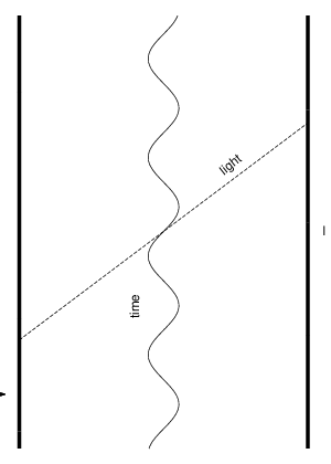

The central part of the diagram, is the position of the throat around which timelike geodesics oscillate. As is seen in Fig.4, the effective potential has a minimum at the throat position, so that the throat attracts the particles. The maximal and minimal values of the radial coordinate, , correspond to the position of the conformal timelike boundary, which is at an infinite proper distance away from the throat. Timelike geodesics are trapped by the confining potential and cannot reach the boundary, while null geodesics () reach it in a finite coordinate time but in an infinite affine time. As a result, the g-geometry is geodesically complete. All this is very similar to the properties of the AdS geometry, apart from the fact that the boundary consists now of two components, and . The conclusion is that timelike geodesics traverse the wormhole and oscillate around the throat.
8.2 Type W1b wormholes
Let us consider the g-geometry shown in Fig.2. The specialty now is that the amplitude vanishes at , where , so that is positive for and is negative otherwise. The 2D part of the metric can be expressed as
| (8.4) |
where the -coordinate is defined by (8.2) for , otherwise one has
| (8.5) |
This determines three coordinate regions:
| (8.6) |
and in the last two regions changes in the opposite directions, so that corresponds to .

In the region one has , so that
| (8.7) |
where . Therefore, the region is conformally equivalent to the diamond in the plane shown in Fig.5. The vertical symmetry axis of the diamond corresponds to the throat position, . In the regions one has either or , hence conformal images of these regions can be obtained by cutting the diamond and keeping either only its right or only its left triangular part, as shown in Fig.5. The vertical side of the triangles then corresponds either to or to , which is the position of the timelike AdS boundary.
The null boundaries of the regions are the Killing horizons. They correspond to but they can be reached by timelike geodesics in a finite proper time. Specifically, the radial timelike geodesics are described by equation (8.3) which can be represented in the equivalent form
| (8.8) |
where is the proper time. Let us denote . The amplitude has a simple zero at and close to this point one has with a constant , in which case Eq.(8.8) yields
| (8.9) |
where is an integration constant. This shows that starting in the region where , the geodesics arrive at the boundary where at a finite moment of the proper time, . Therefore, the region is geodesically incomplete and the geodesics arrive at its null boundary in a finite proper time. The same applies to the regions .
However, it turns out that the boundaries of the regions – the Killing horizons, are singular since the curvature diverges there. Introducing the orthonormal tetrad consisting of the vectors
| (8.10) |
the following tetrad components of the curvature do not vanish (with )
| (8.11) |
Since at the horizon, the components diverge, although this divergence is relatively mild and only leads to finite relative deviations of the neighboring geodesics, and hence to finite tidal deformations. This can be seen by using the equation of the geodesic deviation and integrating over the proper time . However, the component also diverges since when , hence even the 2D metric is singular, even though it reduces in the leading order to the flat Rindler metric . Therefore, every radial geodesic approaching the horizon hits the curvature singularity.
One can nevertheless try and extend the geodesics beyond the horizon in a continuous way, which would allow one to construct a Kruskal-type extension of the metric, although only within the class. Geodesics of the extended metric, after having crossed the horizon, enter a “T-region” where the in Eq.(8.9) formally becomes negative, because space and time interchange their role and the metric becomes
| (8.12) |
Since becomes the timelike coordinate, this metric describes not the static wormhole but rather a dynamical cosmology, a minimum of then corresponding not to the wormhole throat but rather to something like a cosmological bounce. A knowledge of such solutions would allow one to construct a maximal extension of the spacetime geometry in order to find out if the wormhole can be traversed by geodesics or not.
However, solutions in the T-regions are presently not known. In addition, the maximal extension would only be continuous and not differentiable due to the singular nature of the horizons (if there are solutions for which vanishes at the horizon then their extension would be at least ). We therefore do not pursue this line anymore and leave the problem of constructing a maximal extension for the W1b wormhole geometry for a future project.
8.3 Type W2 wormholes
Let us now consider solutions of the type shown in Fig.3. The g-geometry is globally regular and far away from the throat is described by Eq.(5.9), so that in the leading order it approaches the AdS metric with the cosmological constant . As a result, the structure of the g-geometry is essentially the same as for the type W1a solutions. The metric can be cast to the form (8.1), where the conformal coordinate is defined by (8.2) and changes within a finite interval, .
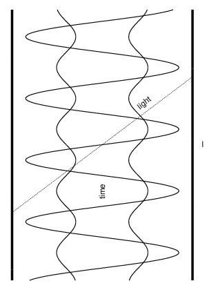

This gives the conformal diagram shown in Fig.6, which is similar to that in Fig.4. The timelike geodesics are described by (8.3), whose potential is shown in Fig.6. The wormhole throat is repulsive, and in addition there is an infinite repulsive barrier at the timelike boundary. As a result, particles with oscillate between the throat and the boundary, while those with traverse the throat and oscillate between the right and left boundaries, as shown in Fig.6.
Let us now consider the f-geometry. Far away from the throat it is described by Eq.(5.9), so that one has asymptotically
| (8.13) |
with a constant . Let us represent the metric as
| (8.14) |
with
| (8.15) |
This radial coordinate changes within a finite range, , because at large one has in view of (8.13) , therefore the integral in (8.15) converges at the upper limit to a finite value . The radial geodesics of the f-metric obey
| (8.16) |
As is seen in Fig.3, the amplitude interpolates between and . Therefore, for large enough there are geodesics which cross the whole range of and arrive at in a finite proper time. When the geometry becomes
| (8.17) |
which is completely regular. As a result, nothing prevents the f-geodesics from extending beyond the values . Hence, from the f-geometry viewpoint, the manifold corresponding to the interval is geodesically incomplete, so that the f-geometry could be extended beyond this interval. However, as far as the g-geometry is concerned, the manifold is complete, because the limiting values correspond to the AdS boundary. We therefore have a peculiar situation where the same manifold is complete in one geometry but is incomplete in the other. One could in principle try and extend the manifold by integrating the equations beyond until the f-geometry is complete. However, the additional parts of the manifold obtained in this way would then be g-geodesically disconnected from the original wormhole, because the latter is already g-complete. We therefore adopt the viewpoint that only the g-metric describes the spacetime geometry, while the f-metric should be viewed as a spin-2 tensor field whose geometric interpretation is possible but not necessary.
9 Concluding remarks
The above analysis gives strong (numerical) evidence in favor of the existence of wormholes in the bigravity theory. These wormholes are very large, with the throat radius of the order of the inverse graviton mass, and they can be of two principal types, which we call W1 and W2.
The W1 wormholes are asymptotically AdS. This feature can be understood by noting that the AdS space is an attractor at large , which means the following. The solutions can be obtained by integrating the system of three first order equations (4.19) for . At large the solutions approach the AdS values, so that
| (9.1) |
where and the deviations are small. Let us consider first the W1a solution shown in Fig.1. Then one has and (see Eqs.(7.2),(7.3)). Linearizing the equations with respect to small then gives the solution
| (9.2) |
where, for the parameter values in (7.1), one finds . The three different values of correspond to three independent solutions, all of them approaching zero as . Therefore, the stable manifold around the AdS fixed point is three-dimensional, so that solutions of the three-dimensional system (4.19) generically run into this fixed point, which is why this is an attractor. For comparison, the flat space is not an attractor since the stable manifold around it is only two-dimensional and the solutions miss it, hence they are not asymptotically flat (probably not even in exceptional cases; see below).
Eq.(9.2) determines the deviation from the AdS asymptotic, ,
| (9.3) |
where are integration constants. The first term on the right here is the contribution of the massless graviton, while the second term is the effect of the scalar polarization of the massive graviton. The embarrassing observation is that the massive contribution oscillates (this is confirmed by the numerics) since given by (9.2) has a non-vanishing imaginary part . This indicates that the mass is imaginary. Indeed, the Fierz-Pauli graviton mass for fluctuations around the proportional AdS background is given by (in units of ) [33]
| (9.4) |
For this gives , hence the gravitons indeed behave as tachyons. The value of the graviton mass actually agrees with the value of given above, which can be seen by noting that the scalar graviton behaves as a scalar field. On the other hand, a static, spherically symmetric scalar field of mass on the AdS background decays asymptotically as with
| (9.5) |
Setting here and choosing the minus sign yields , while setting yields . This reproduces precisely the values in (9.2).
At the same time, one should stress that the very existence of tachyons in the AdS space is not necessarily a bad feature, as long as their mass squared exceeds the BF bound (the mass for which the square root in (9.5) vanishes), in which case they do not produce an instability [36]. However, for the W1a solution shown in Fig.1 one has
| (9.6) |
therefore, the BF bound is violated, which implies that the solution is unstable. It turns out that the BF bound is violated for all W1a solutions that we could find.
On the other hand, for the W1b solution shown in Fig.2 one obtains
| (9.7) |
so that the BF bound is fulfilled, therefore the tachyon instability should be absent. This does not immediately imply that the W1b solutions are stable. However, since they do not suffer from the most dangerous instability, there is a chance that they could be stable, which however can only be decided after a special analysis.
Let us finally consider the W2 wormholes. They do not approach the proportional background and so it is less clear [33] how to compute the Fierz-Pauli mass. However, the linearization of the field equations around the asymptotic values, similar to that described by Eq.(9.1), gives for the deviations power law solutions with real powers. Therefore, there is no evidence for tachyons, so that the W2 solutions could perhaps be stable. It should however be again emphasized that in all cases a detailed stability analysis remains an open issue.
The tachyons [30, 31] and superluminal waves [37, 38, 39] were previously detected in the massive gravity theory with a fixed f-metric. Their existence does not necessarily mean that the theory is ill-defined but rather shows that it can have unphysical solutions. It seems that in the bigravity theory the situation is similar – solutions can be physical and unphysical [40]. The described above W1a wormholes apparently belong to the latter category because they show tachyons and are unstable. One should also say that the solutions may admit a holographic interpretation, similarly to the massive gravity solutions used in the holographic conductivity models [41, 42].
It is instructive to compare the wormholes and black holes [32]. In both cases one can use the Schwarzschild coordinate, For black holes both and vanish at (horizon), while for wormholes vanishes at (throat) but does not. The bigravity black holes [32] are characterized by two independent values, and , and they can be obtained by integrating Eqs.(4.19) for with the boundary condition . The equation (Eq.(4.20)) then insures that , since one generically has at the horizon . Now, the wormholes are actually the same solutions but obtained for special values of (given by Eq.(6.7)) for which the pole of is canceled, and so the equation ensures that is finite as . From this viewpoint, wormholes can be viewed as the special case of black holes corresponding to the fine-tuned .
The bigravity black holes generically approach the AdS space [32], but in exceptional cases, for specially adjusted values of (and for ), they can be asymptotically flat [43]. For the wormholes the value of is already fixed by the condition of having a regular throat, so that one cannot further adjust it to fulfill the asymptotic flatness condition as well. Therefore, asymptotically flat wormholes are unlikely to exist.
The symmetric wormholes exist only in the bigravity and not in the massive gravity theory with a flat f-metric. Indeed, the flat f-metric requires that , which is not compatible with the boundary condition expressed by (6.2). However, we have checked that in the massive gravity limit there are non-symmetric under wormhole-type solutions for which develops a minimum, and even infinitely many minima.
Acknowledgements.
We are grateful to Eugen Radu and Jeorge Rocha and especially to Gary Gibbons for discussions and constructive suggestions. This work was partly supported by the Russian Government Program of Competitive Growth of the Kazan Federal University and also by Grant 14-02-00598 of the Russian Foundation for Basic Research.References
- (1) M. Morris and K. Thorne, Wormholes in space-time and their use for interstellar travel: A tool for teaching general relativity, Am.J.Phys. 56 (1988) 395–412.
- (2) M. Morris, K. Thorne, and U. Yurtsever, Wormholes, Time Machines, and the Weak Energy Condition, Phys.Rev.Lett. 61 (1988) 1446–1449.
- (3) M. Visser, Lorentzian wormholes: From Einstein to Hawking. AIP, 1996.
- (4) D. Hochberg, A. Popov, and S. V. Sushkov, Selfconsistent wormhole solutions of semiclassical gravity, Phys.Rev.Lett. 78 (1997) 2050–2053, [gr-qc/9701064].
- (5) N. R. Khusnutdinov and S. V. Sushkov, Ground state energy in a wormhole space-time, Phys.Rev. D65 (2002) 084028, [hep-th/0202068].
- (6) K. Bronnikov, Scalar-tensor theory and scalar charge, Acta Phys.Polon. B4 (1973) 251–266.
- (7) K. Bronnikov and J. Fabris, Regular phantom black holes, Phys.Rev.Lett. 96 (2006) 251101, [gr-qc/0511109].
- (8) F. S. Lobo, Phantom energy traversable wormholes, Phys.Rev. D71 (2005) 084011, [gr-qc/0502099].
- (9) D. Hochberg, Lorentzian wormholes in higher order gravity theories, Phys.Lett. B251 (1990) 349–354.
- (10) T. Harko, F. S. Lobo, M. Mak, and S. V. Sushkov, Modified-gravity wormholes without exotic matter, Phys.Rev. D87 (2013), no. 6 067504, [arXiv:1301.6878].
- (11) H. Maeda and M. Nozawa, Static and symmetric wormholes respecting energy conditions in Einstein-Gauss-Bonnet gravity, Phys.Rev. D78 (2008) 024005, [arXiv:0803.1704].
- (12) P. Kanti, B. Kleihaus, and J. Kunz, Wormholes in Dilatonic Einstein-Gauss-Bonnet Theory, Phys.Rev.Lett. 107 (2011) 271101, [arXiv:1108.3003].
- (13) P. Kanti, B. Kleihaus, and J. Kunz, Stable Lorentzian Wormholes in Dilatonic Einstein-Gauss-Bonnet Theory, Phys.Rev. D85 (2012) 044007, [arXiv:1111.4049].
- (14) M. R. Mehdizadeh, M. K. Zangeneh, and F. S. N. Lobo, Einstein-Gauss-Bonnet traversable wormholes satisfying the weak energy condition, arXiv:1501.04773.
- (15) K. Bronnikov and S.-W. Kim, Possible wormholes in a brane world, Phys.Rev. D67 (2003) 064027, [gr-qc/0212112].
- (16) G. W. Horndeski, Second-order scalar-tensor field equations in a four-dimensional space, Int.J.Theor.Phys. 10 (1974) 363–384.
- (17) A. B. Balakin, J. P. Lemos, and A. E. Zayats, Nonminimal coupling for the gravitational and electromagnetic fields: Traversable electric wormholes, Phys.Rev. D81 (2010) 084015, [arXiv:1003.4584].
- (18) S. V. Sushkov and R. Korolev, Scalar wormholes with nonminimal derivative coupling, Class.Quant.Grav. 29 (2012) 085008, [arXiv:1111.3415].
- (19) R. Korolev and S. Sushkov, Exact wormhole solutions with nonminimal kinetic coupling, Phys.Rev. D90 (2014), no. 12 124025, [arXiv:1408.1235].
- (20) A. B. Balakin and A. E. Zayats, Dark energy fingerprints in the nonminimal Wu-Yang wormhole structure, Phys.Rev. D90 (2014), no. 4 044049, [arXiv:1408.0862].
- (21) A. Nicolis, R. Rattazzi, and E. Trincherini, The Galileon as a local modification of gravity, Phys.Rev. D79 (2009) 064036, [arXiv:0811.2197].
- (22) C. de Rham, G. Gabadadze, and A. Tolley, Resummation of massive gravity, Phys.Rev.Lett. 106 (2011) 231101, [arXiv:1011.1232].
- (23) K. Hinterbichler, Theoretical aspects of massive gravity, Rev.Mod.Phys. 84 (2012) 671–710, [arXiv:1105.3735].
- (24) C. de Rham, Massive Gravity, Living Rev.Rel. 17 (2014) 7, [arXiv:1401.4173].
- (25) D. Boulware and S. Deser, Can gravitation have a finite range?, Phys.Rev. D6 (1972) 3368–3382.
- (26) M. S. Volkov, Self-accelerating cosmologies and hairy black holes in ghost-free bigravity and massive gravity, Class.Quant.Grav. 30 (2013) 184009, [arXiv:1304.0238].
- (27) M. S. Volkov, Hairy black holes in theories with massive gravitons, Lect.Notes Phys. 892 (2015) 161–180, [arXiv:1405.1742].
- (28) S. Hassan and R. A. Rosen, Bimetric gravity from ghost-free massive gravity, JHEP 1202 (2012) 126, [arXiv:1109.3515].
- (29) V. Baccetti, P. Martin-Moruno, and M. Visser, Null Energy Condition violations in bimetric gravity, JHEP 1208 (2012) 148, [arXiv:1206.3814].
- (30) M. S. Volkov, Stability of Minkowski space in ghost-free massive gravity theory, Phys.Rev. D90 (2014) 024028, [arXiv:1402.2953].
- (31) M. S. Volkov, Energy in ghost-free massive gravity theory, Phys.Rev. D90 (2014), no. 12 124090.
- (32) M. Volkov, Hairy black holes in the ghost-free bigravity theory, Phys.Rev. D85 (2012) 124043, [arXiv:1202.6682].
- (33) S. Hassan, A. Schmidt-May, and M. von Strauss, On Consistent Theories of Massive Spin-2 Fields Coupled to Gravity, JHEP 1305 (2013) 086, [arXiv:1208.1515].
- (34) W. Press, S. Teukolsky, W. Vetterling, and B. Flannery, Numerical Recipes 3rd Edition: The Art of Scientific Computing. Cambridge University Press, New York, NY, USA, 3 ed., 2007.
- (35) C. Deffayet and T. Jacobson, On horizon structure of bimetric spacetimes, Class.Quant.Grav. 29 (2012) 065009, [arXiv:1107.4978].
- (36) P. Breitenlohner and D. Z. Freedman, Positive Energy in anti-De Sitter Backgrounds and Gauged Extended Supergravity, Phys.Lett. B115 (1982) 197.
- (37) S. Deser and A. Waldron, Acausality of Massive Gravity, Phys.Rev.Lett. 110 (2013), no. 11 111101, [arXiv:1212.5835].
- (38) S. Deser, K. Izumi, Y. Ong, and A. Waldron, Massive Gravity Acausality Redux, Phys.Lett. B726 (2013) 544–548, [arXiv:1306.5457].
- (39) S. Deser, M. Sandora, A. Waldron, and G. Zahariade, Covariant constraints for generic massive gravity and analysis of its characteristics, Phys.Rev. D90 (2014), no. 10 104043.
- (40) S. Hassan, A. Schmidt-May, and M. von Strauss, Particular Solutions in Bimetric Theory and Their Implications, Int.Journ.Mod.Phys. 23 (2014) 13, [arXiv:1407.2772].
- (41) M. Blake and D. Tong, Universal Resistivity from Holographic Massive Gravity, Phys.Rev. D88 (2013), no. 10 106004, [arXiv:1308.4970].
- (42) A. Amoretti, A. Braggio, N. Maggiore, N. Magnoli, and D. Musso, Analytic dc thermoelectric conductivities in holography with massive gravitons, Phys.Rev. D91 (2015), no. 2 025002, [arXiv:1407.0306].
- (43) R. Brito, V. Cardoso, and P. Pani, Black holes with massive graviton hair, Phys.Rev. D88 (2013) 064006, [arXiv:1309.0818].