Quintessential inflation with canonical and noncanonical scalar fields and Planck 2015 results
Abstract
We investigate two classes of models of quintessential inflation, based upon canonical as well as noncanonical scalar fields. In particular, introducing potentials steeper than the standard exponential, we construct models that can give rise to a successful inflationary phase, with signatures consistent with Planck 2015 results. Additionally, using nonminimal coupling of the scalar field with massive neutrino matter, we obtain the standard thermal history of the Universe, with late-time cosmic acceleration as the last stage of evolution. In both cases, inflation and late-time acceleration are connected by a tracker solution.
pacs
98.80.-k, 98.80.Cq, 04.50.KdI Introduction
Theoretical and observational consistency demands that the standard model of the Universe should be complemented by an early phase of rapid expansion dubbed inflation [1, 2, 3, 4, 5, 6, 7, 8, 9, 10, 11, 12, 13, 14], as well as by late time cosmic acceleration [15, 16, 17, 18, 19, 20]. The latter is now accepted as a phenomenon of nature supported by independent sets of observations, whereas inflation still awaits similar confirmation. The relic gravitational waves generated quantum-mechanically during inflation would have been a clear and direct signal of inflation [21, 22, 23, 24, 25]. In case the large value of , investigations of B-mode polarization [26] could become a powerful tool to falsify the inflationary paradigm. Unfortunately, the Planck 2015 results [27, 28] seem to further shrink the bound on the tensor-to-scalar ratio of perturbations such that is not ruled out [29, 27, 28].
Needless to say that inflation is one of the most beautiful and simple idea that not only resolves the inconsistencies of the hot big-bang such as the flatness problem, the horizon problem and others, but also provides us with a mechanism of generation of primordial perturbations. As for late time cosmology, the standard model of the Universe is faced with yet another problem related to the age of the Universe, which is a late-time phenomenon [30, 31, 32]. Interestingly, the resolution of the inconsistency within the framework of standard lore, asks for late-time cosmic acceleration, which was indeed confirmed directly by Ia supernovae observations in 1998 [33, 34] and was indirectly supported by other probes independently [35, 36]. Obviously, accelerated expansion plays an important role in the history of Universe, both at its early and late stages.
Often, these two regimes of accelerated expansion are treated independently. However, it is both tempting and economical to think that there is a unique cause responsible for both phases of acceleration à la quintessential inflation [37, 38, 39, 40, 41, 42, 43, 44, 45, 46, 47, 48, 49, 50, 51, 52, 53, 54, 55, 56, 57, 58, 59, 60, 61, 62, 63, 64], which refers to unification of both concepts using a single scalar field. Consistency of the scenario demands that the new degree of freedom, namely the scalar field, should not interfere with the thermal history of the Universe, and thereby it should be “invisible” for the entire evolution and reappear only around the present epoch giving rise to late-time cosmic acceleration. It is, indeed, challenging to build a model which could successfully comply with the said requirements.
First of all, one needs to construct an inflationary phase with a successful exit. Furthermore, in this scenario one needs an alternative reheating method (since the scalar field must survive till late times the conventional reheating is not applicable) and instant preheating [65, 66, 67] is one of the efficient mechanisms that allows conversion of a part of the scalar field energy into radiation. In the post inflationary era till the present epoch, the field potential should be steep, allowing the radiation domination to commence, followed by a thermal history as envisaged by hot big bang. The latter is necessary for sending the field into hiding after the end of inflation. In particular, the post inflationary dynamics is characterized by a field that evolves into the kinetic regime for quite some time, but it then overshoots the background and gets frozen on its potential due to Hubble damping. As the background energy density redshifts to the order of the field energy density, the field resumes its evolution. In case the potential is of a steep exponential form or steeper, the field tracks the background until late times [64]. In case the potential is effectively shallow at late times, the field would exit from the scaling regime to slow roll.
These features look very viable and pleasing, since it is implied that the late time evolution is broadly independent of initial conditions. The main reason for demanding tracker behavior [68] after inflation is related to the hope of alleviation of the fine tuning. However, if we consider the interaction of the scalar field with matter, the mass of the scalar is destabilized, bringing back the same level of fine tuning with the cosmological constant paradigm [64].
In this paper we shall investigate models of quintessential inflation using canonical (Sec. II) as well as noncanonical fields (Sec. III) with tracking behavior. In particular, we are interested in constructing models that can produce a successful inflationary phase (SubSec. II.1 for canonical field and SubSec. III.1 for noncanonical field), with signatures consistent with the Planck 2015 results, and then lead to the standard thermal history of the Universe, with late-time acceleration as the last stage (SubSec. II.2 for canonical field and SubSec. III.2 for noncanonical field). Finally, in Sec IV we summarize our results.
II Unifying inflation and quintessence using a canonical scalar field
In this section we study quintessential inflation using a canonical scalar field. We consider the action
| (1) |
with the Planck mass, the scalar field, and its potential. In the above action we have additionally considered the matter and radiation sectors and respectively. These sectors can be neglected at the inflationary stage, however they will gradually play an important role, giving rise to the standard thermal history of the Universe and finally to the late-time accelerating phase. As usual, we focus on the case of a flat Friedmann-Robertson-Walker (FRW) geometry, with metric
| (2) |
where is the scale factor. Friedman equations are given by
| (3) |
and the equation of motion for the scalar field has the standard form
| (4) |
II.1 Inflation
In what follows, we shall first analyze the inflationary phase in this scenario, focusing on the signatures on the observables that allow for a comparison with the Planck data. As usual, in the inflationary phase one may neglect , and , and thus the dynamics of inflation, as well as its observational signatures, are determined solely by the scalar field and its potential. In particular, given the potential , one introduces the slow-roll parameters
| (5) | |||||
| (6) | |||||
| (7) |
Additionally, the usual condition for ending inflation is simply
| (8) |
where the subscript end represents the value at the end of inflation (we follow the same convention in the rest of the paper). The number of e-foldings is calculated through
| (9) |
Hence, observables like the tensor-to-scalar ratio (), the scalar spectral index () and its running (), can be written as
| (10) | |||||
| (11) | |||||
| (12) |
Keeping in mind the discussion in the introduction, we consider the potential
| (13) |
where and are the usual parameters. Note that compared to standard exponential potential, we have allowed for one more parameter, namely , which would influence the steepness of the potential. The case has been extensively studied in the literature [61, 25, 40, 70, 71, 69] and thus in the following we consider the case . Moreover, we consider the cases and separately, since the corresponding expressions are different in these cases.
II.1.1
In this case the slow-roll parameters (5)-(7) have the following form,
| (14) |
| (15) |
| (16) |
where is the value of the field at the horizon crossing. Additionally, condition (8) gives
| (17) |
and thus from (9) we obtain
| (18) |
One can revert this expression in order to get
| (19) |
with
| (20) |
which allows to eliminate in favor of in the slow-roll parameters. In particular we acquire:
| (21) |
| (22) |
| (23) |
Thus, the tensor-to-scalar ratio (), the scalar spectral index () and its running , can be calculated straightforwardly as functions of using (10)-(12).
Let us now use the above expressions to determine for which combinations of , and e-folding we obtain values of and in agreement with the Planck 2015 results. In particular, we desire to obtain (68 % confidence level, Planck TT,TE,EE+lowP) consistent with the Planck 2015 results [28] and (recent joint analysis of BICEP2/Keck Array and Planck data gives at confidence [29] and when running of the scalar spectral index is allowed Planck 2015 results give [28] at 95 % confidence). As a starting point, and for completeness, we are interested in obtaining , and thus describing the limiting cases of both Collaborations. However, later on we will focus on the low values of this range, in order to obtain agreement with Planck Collaboration [27, 28].
In Fig. 1 we depict the allowed regions in the parameter space that can give [28] and for . We clearly see that the parameter must be larger than .

It is interesting to notice that if we exclude the zero value, for instance if we consider , then the corresponding region is significantly reduced. In Fig. 2 we depict the regions in the parameter space that can give and for and , where the aforementioned feature is clear for . However, this does not seem to be the case according to both 2013 [72] and 2015 [28, 27] Planck data sets. Fig. 2 also shows that the parameter space increases if we increase the value of from 60 to 70.

In order to investigate further the effect of the parameters and , for different e-folding number , on and , we include various figures. Firstly, in Fig. 3 we depict versus , for different values of and e-folding , while in Fig. 4 we show versus , for fixed and different . Similarly, in Fig. 5 we depict versus for different values of and , while in Fig. 6, we show versus , for fixed and different .


It is clear from the above discussion that the scenario at hand, with the potential (13), can give rise to and in agreement with both the Planck 2013 results [72] and the Planck 2015 results [27, 28]. In order to present these features in a more transparent way, in Fig. 7 we depict the predictions of our scenario for varying , and being or , with the e-folding value being or , on top of the 1 and 2 contours of the Planck 2013 results [72] as well as of the Planck 2015 results [27]. As we observe, as or increase, the predictions move towards the core of the data.

Furthermore, in Fig. 8 we present the corresponding situation, but for varying , and being or , with the e-folding value being or . As we observe, as increases the predictions move towards the core of the data.

Hence, we deduce that the larger parametric freedom that was introduced by the use of the additional “steepness” parameter , comparing to models with only the parameter , can lead to the desired - behavior.
For completeness, let us make a comment on the prediction of the scenario at hand on the running spectral index . Using (12) and (21)-(23), we can calculate it for various values of , and , and we present the results on the plane in Fig. 9. On the same graph we depict the 1 and 2 contours of the Planck 2013 results [72] as well as of the Planck 2015 results [27, 28]. As we observe, as or increase the predictions move towards the core of the data, and especially for the parameter values of Figs. 7 and 8 we obtain a remarkable agreement with the Planck 2015 results [27].

Let us now calculate the energy scale of inflation using the COBE normalized value of density perturbations, which can be represented by the following fitting function [73]
| (24) |
On the other hand, the scalar perturbation spectrum is given by
| (25) |
and at the horizon crossing () it becomes
| (26) |
Using Eqs. (24), (25) and (26), we can have the estimation of some model parameters. For instance, for (best fit value of according to [29]), and , equations (10) and (21) give , which leads to . Additionally, for the same values of , the value of the potential at the commencement of inflation is , which provides the scale of inflation as .
Finally, let us discuss on the constraints on reheating temperature from relic gravitational waves. As shown in Refs. [24, 25, 61], the ratio of the energy densities of relic gravitational waves produced during the kinetic regime () and radiation (), is
| (27) |
where “eq” represents the equality of radiation and scalar field energy densities. Moreover, the square of relic gravitational wave amplitude writes as
| (28) |
where is the Hubble parameter at the commencement of inflation, which is .
Nucleosynthesis imposes a constraint on the ratio of the relic gravitational waves and radiation energy densities, namely [36]. Hence, this provides the constraint on the amount of radiation energy density at the end of inflation, that is
| (29) |
Furthermore, the temperature at the end of inflation is . Therefore, using Eq. (29) we can also get a constraint on the temperature at the end of inflation, that is the reheating temperature. If we consider , and , then we have already seen that and . Hence, for these values of the model parameters we get
| (30) |
II.1.2
In this paragraph we present the results in the case for completeness. In this case, the slow-roll parameters (5)-(7) become
| (31) |
Furthermore, the number of e-foldings is
| (32) |
with . Thus, can be expressed through and as , and therefore we can write . Hence, the tensor-to-scalar ratio , the scalar spectral index and its running , are written as
| (33) | |||||
| (34) | |||||
| (35) |
II.2 Late Time Dynamics
In this subsection we investigate the late-time behavior of the above scenario. For usual steep exponential potential () we know that during the post-inflationary dynamics the scalar field rolls down the potential, and its energy density scales as . Due to the increased Hubble damping, the scalar field stops evolving, so its energy density eventually becomes comparable to the background, and it again starts evolving and scales with the background up to late times, thus leaving no place for late-time acceleration. This class of solutions is known as scaling solutions [74]. In Fig. 10 we present such a scaling behavior of the scalar field energy density for an exponential potential.


Now let us see what happens when the potential is steeper than the exponential one, i.e. the case where . Similarly to the exponential potential, in this case too the energy density of the scalar field decreases rapidly, and due to the large Hubble damping the scalar field stops evolving and thus eventually its energy density becomes comparable with the background one. But unlike the exponential case, now, due to the very steep nature of the potential, the scalar field cannot follow the background during the high redshift and thus again . This results in a rapid decrease in the scalar field energy density and hence again the scalar field experiences large Hubble damping due to the background, and therefore it repeats the same behavior as explained earlier (see Fig. 10). However, we mention that this can happen only during large redshifts, where the field value is not so large.
On the other hand, at late times, when the field evolves to a large value, the picture is different. In order to understand the behavior during late times, let us consider the function . For an exponential potential , however for the steeper potential (13) we have,
| (36) |
From this expression it is clear that for large and the function approaches 1, i.e., for asymptotically large field values, the nature of the potential eventually becomes similar to the exponential one. Thus, if at late times the field value is sufficiently large, we obtain a scaling solution, and indeed Fig. 10 confirms this.
Unfortunately, as can be also seen in Fig. 10, we cannot obtain late-time acceleration for the potential (13). In order to achieve late-time acceleration we need a mechanism to exit from the scaling behavior, that is to obtain the tracker behavior [68] at late times. For this purpose we can consider a nonminimal coupling between the scalar field and massive neutrinos, as in Refs. [61, 62, 75] (also see Refs. [79, 80, 81, 82, 83, 84, 85, 76, 86, 87, 77, 88, 78, 89, 90]), and we start with the action:
| (37) |
where
| (38) |
In flat Friedmann-Robertson-Walker (FRW) cosmology the two Friedmann Eqs. (3) modify to:
| (39) | |||
| (40) |
while scalar-field equation (4) now becomes
| (41) |
Before proceeding further we should mention here that massive neutrinos are relativistic () for the most of the expansion history of the Universe and become nonrelativistic () only after the redshift for neutrino mass range [76, 77]. So concerning the neutrino equation-of-state parameter we shall consider the following ansatz [61]:
| (42) |
where and are two parameters which determine the redshift around which the transition of from to 0 starts and how fast the transition happens, respectively and the values of these two parameters depend on the redshift .
Additionally, the continuity equation for massive neutrinos is given by
| (43) |
The last term of Eqs. (41) and (43) is effectively zero when neutrinos behave like radiation, however it becomes non-zero when neutrinos become nonrelativistic (). So the nonminimal coupling between the massive neutrinos and the scalar field affects the expansion of the Universe only during the late times and as can be deduced from (41), an effective potential forms, which reads as
| (44) |
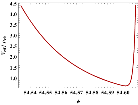
where and are the present values of the field and of the massive neutrino energy density, and . This effective potential clearly has a minimum for , which forms at late times. Hence, the scalar field oscillates around this minimum, and eventually it settles down to the minimum as the oscillations decrease due to the Hubble friction. For clarity, in Fig. 11 we depict the numerically evolved effective potential, normalized by the present critical density (), around its minimum. It should be noted that the minimum value of the effective potential normalized by the present critical density is , which implies that since . Moreover, from Fig. 11 we can see that , where is the energy density of the massive neutrinos at the minimum of the effective potential. Furthermore, from Fig. 11 we observe that . Hence, in summary we can deduce that in the model under consideration the dark energy scale is related to the present energy density of the massive neutrinos.


As we described above, the nonminimal coupling between the scalar field and the neutrinos and the induced effective potential, is adequate to lead to late time acceleration. Indeed, in Fig. 12 we depict the evolution of the various energy densities, and we can clearly see the tracker behavior of the scalar field and the onset of the dark-energy dominating phase.

In order to present the thermal history of the Universe in a more transparent way, we introduce the dimensionless density parameters for matter, radiation, neutrinos and scalar field, respectively given by
| (45) | |||||
| (46) | |||||
| (47) | |||||
| (48) |
where , and in Fig. 13 we depict their evolution as a function of the redshift. As we observe, we can reproduce the thermal history of the Universe, starting from a scalar field kinetic regime, then entering the radiation and matter regimes, and finally resulting to late-time dark-energy dominated era. Finally, for completeness, in Fig. 14 we depict the corresponding behavior of the scalar-field equation-of-state parameter , as well as of the effective (total) equation-of-state parameter . From this figure we verify that around the present era the potential term dominates over the kinetic one in the scalar-field energy density, which leads to be around .


III Unifying inflation and quintessence using a noncanonical scalar field
In this section we shall be interested in constructing quintessential inflation using a class of models with non-canonical scalar field [75, 91, 92, 93, 94, 61, 64] (see also Refs. [95, 96, 97, 98] for unification using noncanonical phantom field). In this case, naturally, we have tracking behaviour in the post inflationary era [61]. Comparing with thawing, the tracking behavior imposes tough restrictions on the post-inflationary evolution of the scalar-field dynamics, namely the field should mimic the background for most of the Universe history, and only at late times it should exit to slow roll regime. The latter is realized only for specific potential forms, otherwise the field exhibits thawing behavior. In summary, in general it is difficult to acquire the tracking features after inflation, using simple potentials. However, the picture changes if we use a scalar field with noncanonical kinetic energy, since in this case it is easy to control the post-inflationary dynamics in the desired way.
Let us consider the following action [75, 61]:
| (49) | |||||
with
| (50) | |||
| (51) | |||
| (52) |
where , , and are the model parameters. The kinetic function has been suitably chosen according to the tracking post-inflationary requirements.
In order to obtain the realistic intervals of the parameter space, we start by noting that in the large-field limit. Thus, in this case we obtain a canonical field with exponential potential, whose slope is given by , which should be large in order to adhere to nucleosynthesis constraint, namely [62]. Similarly, in the small-field limit we can introduce a canonical field , such that the field potential is approximated by , and thereby should be small to comply with inflation [62]. Concerning the parameter , it can be fixed by COBE normalization [62]. Hence, once the post inflationary behavior is guaranteed by the specific form of the kinetic function, inflationary requirements can be obtained through appropriate choices of .
It is clear from the aforesaid that (49) can give rise to a viable model of quintessential inflation by adding a nonminimal coupling between the scalar field and the neutrinos described in subsection II.2. In the following subsection we shall describe inflation using the noncanonical model (49), and we will derive constraints on the model parameters in the light of Planck 2015 results [27, 28]. Finally, in a separate subsection we will examine the late-time, post-inflationary evolution.
III.1 inflation
According to the above discussion, the noncanonical field action (49) can lead to inflation which commences in the small-field region. In particular, the slow-roll parameters can be expressed as [62]
| (53) | |||||
| (54) | |||||
| (55) |
with , and where we have used the approximations and , which should hold in the scenario under consideration. It is clear from (54) that inflation ends in the region with , which quantifies the large-field approximation. In this approximation the number of e-foldings becomes [62]
| (56) |
and thus it can be related to through [62]
| (57) |
Let us note that the transition between small and large field regimes takes place when . Since inflation always ends in the region of large field, its commencement depends upon the range of inflation, which is in turn uniquely specified by the tensor-to-scalar ratio. In particular, a large value of , or weak slow roll, would imply large field excursion. In that case inflation should commence around the boundary of transition, otherwise the commencement would be shifted to the large-field region.
The general expressions for , and the running of spectral index , valid from small to large field regimes are given by
| (58) | |||
| (59) | |||
| (60) |
Hence, let us use these expressions in order to compare the predictions of the scenario at hand with the 2013 and Planck 2015 results. In Fig. 15 we depict the predictions of our model for and e-folding varying between 55 and 70, on top of the 1 and 2 contours of the Planck 2013 results [36] as well as of the Planck 2015 results [27, 28]. As we observe, the point for lies outside the 2 contour of both Planck data sets, but higher values of lie within the 2 contour of both Planck data. Unfortunately, all predictions still lie outside the 1 contour of both data sets, and this becomes worse for larger values of .

As our potential (13) is of unusual form, a comment about the viability of model under quantum correction is in order. Indeed, since, , the model would involve operator of dimensions higher than four if we imagine the series expansion of the potential. It then obviously raises the question whether the model would make sense if quantum corrections are invoked. In general the effective Lagrangian, after we fix the ignorance, contains both renormalizable as well as non-renormalizable parts. As for renormalizable part, it includes one loop corrections to classical Lagrangian. In our case, the latter is absent. The non-renormalizable part includes correction that are suppressed by inverse powers of the cut off. As long as we work quite below the cut off, we can safely use the classical framework. The effective Lagrangian in our case has the form,
| (61) |
where we imagined series expansion of the potential and are constants. In this case, marginal and relevant operators are absent. Thus, in case we work well below the cut off, we can safely ignore the correction and keep using the classical framework.
III.2 Late Time Dynamics
In the noncanonical scalar-field scenario at hand, after the end of inflation the Universe enters into a kinetic-energy-dominated regime, known as “kinetic regime”, and then it subsequently enters into the radiation, matter and dark-energy eras [61]. The nonminimal coupling between the scalar field and massive neutrinos plays the main roll for the onset of late-time cosmic acceleration, as we analyzed in subsection II.2. In particular, when the massive neutrinos become nonrelativistic at late times, they contribute to the formation of the effective potential with a minimum. As a result, the scalar field settles down to the minimum of the effective potential after damping of oscillations which ultimately gives rise to the late time acceleration. For a detailed dynamical analysis one can see Ref. [61]. The late-time attractor solution corresponds to an effective (total) equation-of-state parameter given by [61]
| (62) |
and to a scalar-field equation of state
| (63) |
where is the canonical scalar field which can be represented in terms of the noncanonical scalar field using the transformation [61]
| (64) | |||||
| (65) |
From (63) we can see that if , i.e. without a coupling between the scalar field and massive neutrinos, , which implies that the scalar field will exhibit scaling behavior even during late times, and will continue to follow the background even in the future. Hence, we do verify what we discussed earlier, namely that in the absence of the nonminimal coupling we cannot acquire late-time acceleration. On the other hand, from (62) we deduce that in order to obtain a de Sitter or nearly de Sitter solution () we require . Thus, a large nonminimal coupling is needed in order to acquire late-time acceleration.
Finally, note that the value of the effective potential at the minimum is directly proportional to the present neutrino energy density [61, 64]. Therefore, the dark energy scale is related to the neutrino energy scale, similarly to the analysis of Section II. Hence, the nonminimal coupling between the scalar field and massive neutrinos not only provides the late-time acceleration, but it additionally fixes the energy scale of dark energy.
IV Conclusions
In this work we investigated two distinct classes of quintessential inflation, namely models based on a canonical scalar-field and models based on a noncanonical scalar field, where both scenarios exhibit tracking behavior. In both cases we considered a nonminimal coupling between the scalar field and the neutrinos, which is required in order to trigger the late-time cosmic acceleration.
In the canonical case we considered a potential of the form , with , which has the property of slow roll near the origin but it becomes steep away from it. Hence, at early times, i.e. while the field is around the origin, this scenario can give rise to inflation. Indeed, as we demonstrated in Figs. 1 and 2, for a range of the model parameters we can obtain a required phase of inflation with the spectral index and the tensor-to-scalar ratio in a very good agreement with the Planck 2015 results [27, 28] and the joint analysis of BICEP2/Keck Array and Planck data [29]. Indeed, in Fig. 7 and Fig. 8 we showed that the predictions of the scenario fall well inside the 1 likelihood contours of both Planck 2013 results [72] and Planck 2015 results [28, 27]. Additionally, for the representative case of the parameter choice , and e-foldings , the obtained provides the estimate or equivalently the scale of inflation, . Finally, using nucleosynthesis constraints we obtained the lower bound on the temperature at the end of inflation, namely .
After the end of inflation, the steep potential derives the scalar field into the kinetic regime. Consequently, the field overshoots the background and freezes due to Hubble damping. The evolution of the field resumes soon after the background energy density becomes comparable to field energy density. In the usual case of exponential potential () the field follows scaling behavior. In the case of , the potential is steeper than the standard exponential and thus the field is driven away from the scaling track, which increases the Hubble damping leading to the freezing of the field once again. As the field comes out of the freezing regime, its energy density redshifts faster than the background, and this feature brings back the Hubble damping and so on. The said behavior keeps repeating till the field acquires large values. In that case and the field enters the regime which is an attractor, see Fig. 10. The latter allows us to obtain the subsequent radiation and matter regimes. Thus, we conclude that the scaling solution is also an attractor in case the potential is steeper than a standard steep exponential. To the best of our knowledge, this feature was not noted earlier in the literature. In case of generic values of and , the field rolls in the domain of large in the post inflationary era in which case the system enters into the tracking regime after the Hubble freezing ends, see Fig. 12.
Finally, the nonminimal coupling between the scalar field and the neutrinos induces an effective potential, which leads the scalar field to drive the late-time acceleration. The larger the nonminimal coupling is, the deeper the minimum of the effective potential is, in which the field is settled after damped oscillations, exhibiting an equation-of-state parameter around in the present epoch.
As for the noncanonical scalar field, although both inflation and the subsequent thermal history of the Universe, including late-time acceleration, can be obtained, the specific values of the spectral index and of the tensor-to-scalar ratio are not in complete agreement with the Planck 2015 results [27, 28].
In this work we showed that using potentials steeper than the exponential we can solve the problem of models of quintessential inflation which give rise to numerical values of larger than the Planck bounds [27, 28], and we can obtain a remarkable agreement with the Planck 2015 results [27, 28]. We have shown that it is possible to reproduce the correct post-inflationary evolution during radiation and matter eras. The nonminimal coupling between the scalar field and the neutrinos is shown to drive the late-time cosmic acceleration. To summarize, we presented a successful model of quintessential inflation that can describe the entire history of Universe evolution in a unified framework.
Acknowledgements.
M.W.H. acknowledges CSIR, Govt. of India for financial support through SRF scheme (File No:09/466(0128)/2010-EMR-I). The research of ENS is implemented within the framework of the Action “Supporting Postdoctoral Researchers” of the Operational Program “Education and Lifelong Learning” (Actions Beneficiary: General Secretariat for Research and Technology), and is co-financed by the European Social Fund (ESF) and the Greek State.References
- [1] A. A. Starobinsky, Phys. Lett. B 91, 99 (1980).
- [2] A. A. Starobinsky, Phys. Lett. B 117, 175 (1982).
- [3] A. H. Guth, Phys. Rev. D 23, 347 (1981).
- [4] A. D. Linde, Phys. Lett. B 129, 177 (1983).
- [5] A. D. Linde, Phys. Lett. B 108, 389 (1982).
- [6] A. R. Liddle, [astro-ph/9901124].
- [7] D. Langlois, [hep-th/0405053].
- [8] D. H. Lyth and A. Riotto, Phys. Rept. 314, 1 (1999) [hep-ph/9807278].
- [9] A. H. Guth, Phys. Rept. 333, 555 (2000) [as tro-ph/0002156].
- [10] J. E. Lidsey, A. R. Liddle, E. W. Kolb, E. J. Copeland, T. Barreiro and M. Abney, Rev. Mod. Phys. 69, 373 (1997) [astro-ph/9508078].
- [11] B. A. Bassett, S. Tsujikawa and D. Wands, Rev. Mod. Phys. 78, 537 (2006) [astro-ph/0507632].
- [12] A. Mazumdar and J. Rocher, Phys. Rept. 497, 85 (2011) [arXiv:1001.0993 [hep-ph]].
- [13] L. Wang, E. Pukartas and A. Mazumdar, JCAP 1307, 019 (2013) [arXiv:1303.5351 [hep-ph]].
- [14] A. Mazumdar and B. Zaldivar, [arXiv:1310.5143 [hep-ph]].
- [15] P. J. E. Peebles and B. Ratra, Rev. Mod. Phys. 75, 559 (2003) [astro-ph/0207347].
- [16] E. J. Copeland, M. Sami and S. Tsujikawa, Int. J. Mod. Phys. D 15, 1753 (2006) [hep-th/0603057].
- [17] V. Sahni and A. A. Starobinsky, Int. J. Mod. Phys. D 9, 373 (2000) [astro-ph/9904398].
- [18] T. Padmanabhan, AIP Conf. Proc. 861, 179 (2006) [as tro-ph/0603114].
- [19] J. Frieman, M. Turner and D. Huterer, Ann. Rev. Astron. Astrophys. 46, 385 (2008) [arXiv:0803.0982 [astro-ph]].
- [20] Y. F. Cai, E. N. Saridakis, M. R. Setare and J. Q. Xia, Phys. Rept. 493, 1 (2010) [arXiv:0909.2776 [hep-th]].
- [21] L. P. Grishchuk, Sov. Phys. JETP 40, 409 (1975) [Zh. Eksp. Teor. Fiz. 67, 825 (1974)].
- [22] A. A. Starobinsky, JETP Lett. 30, 682 (1979) [Pisma Zh. Eksp. Teor. Fiz. 30, 719 (1979)].
- [23] B. Allen, Phys. Rev. D 37, 2078 (1988).
- [24] V. Sahni, Phys. Rev. D 42, 453 (1990).
- [25] V. Sahni, M. Sami and T. Souradeep, Phys. Rev. D 65, 023518 (2001) [gr-qc/0105121].
- [26] P. A. R. Ade et al. [BICEP2 Collaboration], Phys. Rev. Lett. 112, 241101 (2014), arXiv:1403.3985 [astro-ph.CO].
- [27] [Planck Collaboration], arXiv:1502.01589 [astro-ph.CO].
- [28] P. A. R. Ade et al. [Planck Collaboration], arXiv:1502.02114 [astro-ph.CO].
- [29] P. A. R. Ade et al. [BICEP2 and Planck Collaborations], [arXiv:1502.00612 [astro-ph.CO]].
- [30] L. M. Krauss and M. S. Turner, Gen. Rel. Grav. 27, 1137 (1995) [astro-ph/9504003].
- [31] M. S. Turner, astro-ph/9703161.
- [32] Krauss, L.M., Chaboyer, B., Science 229, 65 (2003).
- [33] A. G. Riess et al. [Supernova Search Team Collabora tion], Astron. J. 116, 1009 (1998) [astro-ph/9805201].
- [34] S. Perlmutter et al. [Supernova Cosmology Project Collaboration], Astrophys. J. 517, 565 (1999) [as tro-ph/9812133].
- [35] C. L. Bennett et al. [WMAP Collaboration], Astrophys. J. Suppl. 148, 1 (2003) [astro-ph/0302207].
- [36] P. A. R. Ade et al. [Planck Collaboration], Astron. As trophys. (2014) [arXiv:1303.5076 [astro- ph.CO]].
- [37] P. J. E. Peebles and A. Vilenkin, Phys. Rev. D 60,103506 (1999) [astro-ph/9904396].
- [38] M. Sami and V. Sahni, Phys. Rev. D 70, 083513 (2004) [hep-th/0402086].
- [39] M. Sami and N. Dadhich, TSPU Vestnik 44N7, 25 (2004), [hep-th/0405016].
- [40] E. J. Copeland, A. R. Liddle and J. E. Lidsey, Phys. Rev. D 64, 023509 (2001) [astro-ph/0006421].
- [41] G. Huey and J. E. Lidsey, Phys. Lett. B 514, 217 (2001) [astro-ph/0104006].
- [42] K. Dimopoulos, Nucl. Phys. Proc. Suppl. 95, 70 (2001) [astro-ph/0012298].
- [43] M. Sami, N. Dadhich and T. Shiromizu, Phys. Lett. B 568, 118 (2003) [hep-th/0304187].
- [44] M. Dias and A. R. Liddle, Phys. Rev. D 81, 083515 (2010) [1002.3703 [astro-ph.CO]].
- [45] M. Bastero-Gil, A. Berera, B. M. Jackson and A. Taylor, Phys. Lett. B 678, 157 (2009) [0905.2937 [hep-ph]].
- [46] E. J. Chun, S. Scopel and I. Zaballa, JCAP 0907, 022 (2009) [0904.0675 [hep-ph]].
- [47] M. C. Bento, R. G. Felipe and N. M. C. Santos, Phys. Rev. D 77, 123512 (2008) [0801.3450 [astro-ph]].
- [48] I. P. Neupane, Class. Quant. Grav. 25, 125013 (2008) [0706.2654 [hep-th]].
- [49] R. Rosenfeld and J. A. Frieman, Phys. Rev. D 75, 043513 (2007) [astro-ph/0611241].
- [50] A. Membiela and M. Bellini, Phys. Lett. B 641, 125 (2006) [gr-qc/0606119].
- [51] J. C. Bueno Sanchez and K. Dimopoulos, Phys. Lett. B 642, 294 (2006) [Erratum-ibid. B 647, 526 (2007)] [hep-th/0605258].
- [52] V. H. Cardenas, Phys. Rev. D 73, 103512 (2006) [gr-qc/0603013].
- [53] X. -h. Zhai and Y. -b. Zhao, Chin. Phys. 15, 2465 (2006) [astro-ph/0511512].
- [54] R. Rosenfeld and J. A. Frieman, JCAP 0509, 003 (2005) [astro-ph/0504191].
- [55] M. Giovannini, Phys. Rev. D 67, 123512 (2003) [hep- ph/0301264].
- [56] N. J. Nunes and E. J. Copeland, Phys. Rev. D 66, 043524 (2002) [astro-ph/0204115].
- [57] K. Dimopoulos and J. W. F. Valle, Astropart. Phys. 18, 287 (2002) [astro-ph/0111417].
- [58] M. Yahiro, G. J. Mathews, K. Ichiki, T. Kajino and M. Orito, Phys. Rev. D 65, 063502 (2002) [as tro-ph/0106349].
- [59] A. B. Kaganovich, Phys. Rev. D 63, 025022 (2000) [hep- th/0007144].
- [60] M. Peloso and F. Rosati, JHEP 9912, 026 (1999) [hep- ph/9908271].
- [61] M. W. Hossain, R. Myrzakulov, M. Sami and E. N. Saridakis, Phys. Rev. D 90, 023512 (2014) [1402.6661 [gr-qc]].
- [62] M. W. Hossain, R. Myrzakulov, M. Sami and E. N. Saridakis, Phys. Rev. D 89, 123513 (2014) [1404.1445 [gr-qc]].
- [63] M. W. Hossain, R. Myrzakulov, M. Sami and E. N. Saridakis, Phys. Lett. B 737, 191 (2014) [arXiv:1405.7491 [gr-qc]].
- [64] M. W. Hossain, R. Myrzakulov, M. Sami and E. N. Saridakis, [arXiv:1410.6100 [gr-qc]].
- [65] G. N. Felder, L. Kofman and A. D. Linde, Phys. Rev. D 59, 123523 (1999) [hep-ph/9812289].
- [66] G. N. Felder, L. Kofman and A. D. Linde, Phys. Rev. D 60, 103505 (1999) [hep-ph/9903350].
- [67] A. H. Campos, J. M. F. Maia and R. Rosenfeld, Phys. Rev. D 70, 023003 (2004) [astro-ph/0402413].
- [68] P. J. Steinhardt, L. M. Wang and I. Zlatev, Phys. Rev. D 59, 123504 (1999) [astro-ph/9812313].
- [69] F. Lucchin and S. Matarrese, Phys. Rev. D 32, 1316 (1985).
- [70] B. Ratra, Phys. Rev. D 45, 1913 (1992).
- [71] M. Sami, P. Chingangbam and T. Qureshi, Phys. Rev. D 66, 043530 (2002) [hep-th/0205179].
- [72] P. A. R. Ade et al. [Planck Collaboration], Astron. Astro phys. 571, A22 (2014) [arXiv:1303.5082 [astro-ph.CO]].
- [73] E. F. Bunn, A. R. Liddle and M. J. White, 1, Phys. Rev. D 54, 5917 (1996) [astro-ph/9607038].
- [74] E. J. Copeland, A. R. Liddle and D. Wands, Phys. Rev. D 57, 4686 (1998) [gr-qc/9711068].
- [75] C. Wetterich, Phys. Rev. D 89, 024005 (2014) [1308.1019[astro-ph.CO]].
- [76] L. Amendola, M. Baldi and C. Wetterich, Phys. Rev. D 78, 023015 (2008) [arXiv:0706.3064 [astro-ph]].
- [77] C. Wetterich, Phys. Lett. B 655, 201 (2007) [arXiv:0706.4427 [hep-ph]].
- [78] V. Pettorino, N. Wintergerst, L. Amendola and C. Wetterich, Phys. Rev. D 82, 123001 (2010) [arXiv:1009.2461[astro-ph.CO]].
- [79] R. Fardon, A. E. Nelson and N. Weiner, JCAP 0410, 005 (2004) [astro-ph/0309800].
- [80] X. -J. Bi, P. -h. Gu, X. -l. Wang and X. -m. Zhang, Phys. Rev. D 69, 113007 (2004) [hep-ph/0311022].
- [81] P. Q. Hung and H. Pas, Mod. Phys. Lett. A 20, 1209 (2005) [astro-ph/0311131].
- [82] R. D. Peccei, Phys. Rev. D 71, 023527 (2005) [hep- ph/0411137].
- [83] X. -J. Bi, B. Feng, H. Li and X. -m. Zhang, Phys. Rev. D 72, 123523 (2005) [hep-ph/0412002].
- [84] A. W. Brookfield, C. van de Bruck, D. F. Mota and D. Tocchini-Valentini, Phys. Rev. Lett. 96, 061301 (2006) [astro-ph/0503349].
- [85] A. W. Brookfield, C. van de Bruck, D. F. Mota and D. Tocchini-Valentini, Phys. Rev. D 73, 083515 (2006) [Erratum-ibid. D 76, 049901 (2007)] [astro-ph/0512367].
- [86] O. E. Bjaelde, A. W. Brookfield, C. van de Bruck, S. Hannestad, D. F. Mota, L. Schrempp and D. Tocchini-Valentini, JCAP 0801, 026 (2008) [arXiv:0705.2018 [astro-ph]].
- [87] N. Afshordi, M. Zaldarriaga and K. Kohri, Phys. Rev. D 72, 065024 (2005) [astro-ph/0506663].
- [88] D. F. Mota, V. Pettorino, G. Robbers and C. Wetterich, Phys. Lett. B 663, 160 (2008) [arXiv:0802.1515 [astro-ph]].
- [89] G. La Vacca and D. F. Mota, Astron. Astrophys. 560, A53 (2013) [arXiv:1205.6059 [astro-ph.CO]].
- [90] L. G. Collodel and G. M. Kremer, Grav. Cosmol. 18, 196 (2012) [arXiv:1203.3061 [gr-qc]].
- [91] C. Wetterich, Physics of the Dark Universe (2013), [arXiv:1303.6878 [astro-ph.CO]].
- [92] C. Wetterich, Phys. Lett. B 726, 15 (2013) [arXiv:1303.4700 [astro-ph.CO]].
- [93] C. Wetterich, Phys. Lett. B 736, 506 (2014) [arXiv:1401.5313 [astro-ph.CO]].
- [94] C. Wetterich, Lecture Notes in Physics Volume 892, 2015, pp 57-95 [arXiv:1402.5031 [astro-ph.CO]].
- [95] S. ’i. Nojiri and S. D. Odintsov, Gen. Rel. Grav. 38, 1285 (2006) [hep-th/0506212].
- [96] S. Capozziello, S. Nojiri and S. D. Odintsov, Phys. Lett. B 632, 597 (2006) [hep-th/0507182].
- [97] E. Elizalde, S. Nojiri, S. D. Odintsov, D. Saez-Gomez and V. Faraoni, Phys. Rev. D 77, 106005 (2008) [arXiv:0803.1311 [hep-th]].
- [98] Y. Ito, S. Nojiri and S. D. Odintsov, Entropy 14, 1578 (2012) [arXiv:1111.5389 [hep-th]].