跳到论文正文
W Papers独立论文阅读器 arXiv:1502.03470 论文正文 计算阅读时间 · 0%
引用这篇论文根据当前论文元数据生成,正式投稿前建议核对。


License: arXiv.org perpetual non-exclusive license
arXiv:1502.03470v2 [math.PR] 02 Nov 2015

Two-dimensional random interlacements and late points for random walks

Francis Comets    Serguei Popov    Marina Vachkovskaia
Abstract

We define the model of two-dimensional random interlacements using simple random walk trajectories conditioned on never hitting the origin, and then obtain some properties of this model. Also, for random walk on a large torus conditioned on not hitting the origin up to some time proportional to the mean cover time, we show that the law of the vacant set around the origin is close to that of random interlacements at the corresponding level. Thus, this new model provides a way to understand the structure of the set of late points of the covering process from a microscopic point of view.
Keywords: random interlacements, hitting time, simple random walk, Doob’s hh-transform
AMS 2010 subject classifications: Primary 60K35. Secondary 60G50, 82C41.

1{}^{~1}Université Paris Diderot – Paris 7, Mathématiques, case 7012, F–75205 Paris Cedex 13, France
e-mail: comets@math.univ-paris-diderot.fr

2{}^{~2}Department of Statistics, Institute of Mathematics, Statistics and Scientific Computation, University of Campinas – UNICAMP, rua Sérgio Buarque de Holanda 651, 13083–859, Campinas SP, Brazil
e-mails: {popov,marinav}@ime.unicamp.br

1 Introduction

We start by an informal description of our purpose.

1.1 Random interlacements in two dimensions

Random interlacements were introduced by Sznitman in [20], motivated by the problem of disconnection of the discrete torus ℤnd:=ℤd/n​ℤd{\mathbb{Z}}_{n}^{d}:={\mathbb{Z}}^{d}/n{\mathbb{Z}}^{d} by the trace of simple random walk, in dimension 33 or higher. Detailed accounts can be found in the survey [4] and the recent book [10]. Loosely speaking, the model of random interlacements in ℤd{\mathbb{Z}}^{d}, d≥3d\geq 3, is a stationary Poissonian soup of (transient) doubly infinite simple random walk trajectories on the integer lattice. There is an additional parameter u>0u>0 entering the intensity measure of the Poisson process, the larger uu is the more trajectories are thrown in. The sites of ℤd{\mathbb{Z}}^{d} that are not touched by the trajectories constitute the vacant set 𝒱u{\mathcal{V}}^{u}. The random interlacements are constructed simultaneously for all u>0u>0 in such a way that 𝒱u1⊂𝒱u2{\mathcal{V}}^{u_{1}}\subset{\mathcal{V}}^{u_{2}} if u1>u2u_{1}>u_{2}. In fact, the law of the vacant set at level uu can be uniquely characterized by the following identity:

ℙ[A⊂𝒱u]=exp(−ucap(A))for all finite A⊂ℤd,{\mathbb{P}}[A\subset{\mathcal{V}}^{u}]=\exp\big(-u\mathop{\mathrm{cap}}(A)\big)\quad\text{for all finite $A\subset{\mathbb{Z}}^{d}$}, (1)

where cap(A)\mathop{\mathrm{cap}}(A) is the capacity of AA. Informally, the capacity measures how “big” the set is from the point of view of the walk, see Section 6.5 of [13] for formal definitions, as well as (13)–(14) below.

At first glance, the title of this section seems to be meaningless, just because even a single trajectory of two-dimensional simple random walk a.s. visits all sites of ℤ2{\mathbb{Z}}^{2}, so the vacant set would be always empty. Nevertheless, there is also a natural notion of capacity in two dimensions (cf. Section 6.6 of [13]), so one may wonder if there is a way to construct a decreasing family (𝒱α,α>0)({\mathcal{V}}^{\alpha},\alpha>0) of random subsets of ℤ2{\mathbb{Z}}^{2} in such a way that a formula analogous to (1) holds for every finite AA. This is, however, clearly not possible since the two-dimensional capacity of one-point sets equals 00. On the other hand, it turns out to be possible to construct such a family so that

ℙ[A⊂𝒱α]=exp(−παcap(A)){\mathbb{P}}[A\subset{\mathcal{V}}^{\alpha}]=\exp\big(-\pi\alpha\mathop{\mathrm{cap}}(A)\big) (2)

holds for all sets containing the origin (the factor π\pi in the exponent is just for convenience, as explained below). We present this construction in Section 2.1. To build the interlacements, we use trajectories of simple random walks conditioned on never hitting the origin. Of course, the law of the vacant set is no longer translationally invariant, but we show that it has the property of conditional translation invariance, cf. Theorem 2.3 below. In addition, we will see that (similarly to the d≥3d\geq 3 case) the random object we construct has strong connections to random walks on two-dimensional torus. All this makes us believe that “two-dimensional random interlacements” is the right term for the object we introduce in this paper.

1.2 Cover time and late points of simple random walk on a discrete torus

Consider the simple random walk on the two-dimensional discrete torus ℤn2{\mathbb{Z}}^{2}_{n} with the starting point chosen uniformly at random. Let 𝒯n{\mathcal{T}}_{n} be the first moment when this random walk visits all sites of ℤn2{\mathbb{Z}}^{2}_{n}; we refer to 𝒯n{\mathcal{T}}_{n} as the cover time of the torus. It was shown in [7] that 𝒯nn2​ln2​n→4π\frac{{\mathcal{T}}_{n}}{n^{2}\ln^{2}n}\to\frac{4}{\pi} in probability; later, this result was refined in [9], and then even finer results on the first correction to this limit were obtained in [2] for the similar problem of covering the (continuous) torus with a Brownian sausage.

The structure of the set of late points (i.e., the set of points that are still unvisited up to a given time) of the random walk on the torus is rather well understood in dimensions d≥3d\geq 3, see [1, 15], and also  [12] for the continuous case. On the other hand, much remains to be discovered in two dimensions. After the heuristic arguments of [3] revealing an intriguing random set, it was shown in [8] that this set has interesting fractal-like properties when the elapsed time is a fraction of the expected cover time. This particular behaviour is induced by long distance correlations between hitting times due to recurrence. In this paper, we prove that the law of the uncovered set around the origin at time 4​απ​n2​ln2​n\frac{4\alpha}{\pi}n^{2}\ln^{2}n conditioned on the event that the origin is uncovered, is close to the law of two-dimensional random interlacements at level α\alpha (Theorem 2.6). We hope that this result will lead to other advances in understanding the structure of the uncovered set.

We now explain why conditioning is necessary to observe a meaningful point process. In two dimensions, if we know that simple random walk has visited a given site by a large time, then it is likely, by recurrence, that it has has visited all the nearby sites as well. This means that a fixed-size window around the origin will be typically either full (on the event that the origin was visited) or empty (if the origin was not yet visited). Therefore, we need to condition on a rare event to obtain a nontrivial limit.

As a side note, observe that the two-dimensional random interlacements relate to the simple random walk on the torus at a time proportional to the cover time. In higher dimensions, one starts to observe the “interlacement regime” already at times below the cover time by a factor of ln⁡n\ln n.

Organisation of the paper: In Section 2.1 we construct the model of random interlacements and present some of its properties. In Section 2.2 we formulate a result relating this model and the vacant set of the simple random walk on the discrete torus. We prove some results on the spot – when short arguments are available – postponing the proof of the other ones to Section 4. Section 3 contains a number of auxiliary facts needed for the proof of the main results.

2 Definitions and results

We start by defining the two-dimensional random interlacement process, which involves some potential-theoretic considerations.

2.1 Random interlacements: definitions, properties

Let ∥⋅∥\|\cdot\| be the Euclidean norm. Define the (discrete) ball

B⁡(x,r)={y∈ℤ2:‖y−x‖≤r}B(x,r)=\{y\in{\mathbb{Z}}^{2}:\|y-x\|\leq r\}

(note that xx and rr need not be integer), and abbreviate B⁡(r):=B⁡(0,r)B(r):=B(0,r). We write x∼yx\sim y if xx and yy are neighbours on ℤ2{\mathbb{Z}}^{2}. The (internal) boundary of A⊂ℤ2A\subset{\mathbb{Z}}^{2} is defined by

∂A={x∈A:there exists ​y∈ℤ2∖A​ such that ​x∼y}.\partial A=\{x\in A:\text{there exists }y\in{\mathbb{Z}}^{2}\setminus A\text{ such that }x\sim y\}.

Let (Sn,n≥0)(S_{n},n\geq 0) be two-dimensional simple random walk. Write PxP_{x} for the law of the walk started from xx and ExE_{x} for the corresponding expectation. Let

τ0​(A)\displaystyle\tau_{0}(A) =inf{k≥0:Sk∈A},\displaystyle=\inf\{k\geq 0:S_{k}\in A\}, (3)
τ1​(A)\displaystyle\tau_{1}(A) =inf{k≥1:Sk∈A}\displaystyle=\inf\{k\geq 1:S_{k}\in A\} (4)

be the entrance and the hitting time of the set AA by simple random walk SS (we use the convention inf∅=+∞\inf\emptyset=+{\infty}). For a singleton A={x}A=\{x\}, we will write τi​(A)=τi​(x)\tau_{i}(A)=\tau_{i}(x), i=0,1i=0,1, for short. Define the potential kernel aa by

a(x)=∑k=0∞(P0[Sk=0]−Px[Sk=0]).a(x)=\sum_{k=0}^{\infty}\big(P_{0}[S_{k}\!=\!0]-P_{x}[S_{k}\!=\!0]\big). (5)

It can be shown that the above series indeed converges and we have a⁡(0)=0a(0)=0, a⁡(x)>0a(x)>0 for x≠0x\neq 0, and

a⁡(x)=2π​ln⁡‖x‖+γ′+O⁡(‖x‖−2)a(x)=\frac{2}{\pi}\ln\|x\|+\gamma^{\prime}+O(\|x\|^{-2}) (6)

as x→∞x\to\infty, cf. Theorem 4.4.4 of [13] (the value of γ′\gamma^{\prime} is known11 1 γ′=π−1​(2​γ+ln⁡8)\gamma^{\prime}=\pi^{-1}(2\gamma+\ln 8), where γ=0.5772156​…\gamma=0.5772156\dots is the Euler-Mascheroni constant, but we will not need it in this paper). Also, the function aa is harmonic outside the origin, i.e.,

14∑y:y∼xa(y)=a(x) for all x≠0.\frac{1}{4}\sum_{y:y\sim x}a(y)=a(x)\quad\text{ for all }x\neq 0. (7)

Observe that (7) immediately implies that a⁡(Sk∧τ0​(0))a(S_{k\wedge\tau_{0}(0)}) is a martingale, we will repeatedly use this fact in the sequel. With some abuse of notation, we also consider the function

a⁡(r)=2π​ln⁡r+γ′a(r)=\frac{2}{\pi}\ln r+\gamma^{\prime}

of a real argument r≥1r\geq 1. The advantage of using this notation is e.g. that, due to (6), we may write, as r→∞r\to\infty,

∑y∈∂B⁡(x,r)ν⁡(y)​a​(y)=a⁡(r)+O⁡(‖x‖∨1r)\sum_{y\in\partial B(x,r)}\nu(y)a(y)=a(r)+O\Big(\frac{\|x\|\vee 1}{r}\Big) (8)

for any probability measure ν\nu on ∂B⁡(x,r)\partial B(x,r). The harmonic measure of a finite A⊂ℤ2A\subset{\mathbb{Z}}^{2} is the entrance law “starting at infinity”,

hmA(x)=lim‖y‖→∞Py[Sτ1​(A)=x].\mathop{\mathrm{hm}}\nolimits_{A}(x)=\lim_{\|y\|\to\infty}P_{y}[S_{\tau_{1}(A)}=x]. (9)

The existence of the above limit follows from Proposition 6.6.1 of [13]; also, this proposition together with (6.44) implies that

hmA(x)=2πlimR→∞Px[τ1(A)>τ1(∂B(R))]lnR.\mathop{\mathrm{hm}}\nolimits_{A}(x)=\frac{2}{\pi}\lim_{R\to\infty}P_{x}\big[\tau_{1}(A)>\tau_{1}\big(\partial B(R)\big)\big]\ln R. (10)

Intuitively, (10) means that the harmonic measure at x∈∂Ax\in\partial A is proportional to the probability of escaping from xx to a large sphere. Observe also that, by recurrence of the walk, hmA\mathop{\mathrm{hm}}\nolimits_{A} is a probability measure on ∂A\partial A. Now, for a finite set AA containing the origin, we define its capacity by

cap(A)=∑x∈Aa⁡(x)​hmA(x);\mathop{\mathrm{cap}}(A)=\sum_{x\in A}a(x)\mathop{\mathrm{hm}}\nolimits_{A}(x); (11)

in particular, cap({0})=0\mathop{\mathrm{cap}}\big(\{0\}\big)=0 since a⁡(0)=0a(0)=0. For a set not containing the origin, its capacity is defined as the capacity of a translate of this set that does contain the origin. Indeed, it can be shown that the capacity does not depend on the choice of the translation. A number of alternative definitions are available, cf. Section 6.6 of [13]. Intuitively, the capacity of AA represents the difference in size between the set AA and a single point, as seen from infinity: From (6.40) and the formula above Proposition 6.6.2 in [13], we can write

Px[τ1(∂B(r))<τ1(A)]=ln⁡‖x‖+π​γ′2−π2​cap(A)+εA​(x)+εA,x′​(r)ln⁡r,P_{x}\big[\tau_{1}\big(\partial B(r)\big)<\tau_{1}(A)\big]=\frac{\ln\|x\|+\frac{\pi\gamma^{\prime}}{2}-\frac{\pi}{2}\mathop{\mathrm{cap}}(A)+\varepsilon_{A}(x)+\varepsilon_{A,x}^{\prime}(r)}{\ln r},

where εA​(x)\varepsilon_{A}(x) vanishes as ‖x‖→∞\|x\|\to{\infty} and εA,x′​(r)\varepsilon_{A,x}^{\prime}(r) vanishes as r→∞r\to{\infty} keeping fixed the other variables. Observe that, by symmetry, the harmonic measure of any two-point set is uniform, so cap({x,y})=12​a​(y−x)\mathop{\mathrm{cap}}\big(\{x,y\}\big)=\frac{1}{2}a(y-x) for any x,y∈ℤ2x,y\in{\mathbb{Z}}^{2}. Also, (8) implies that

cap(B⁡(r))=a⁡(r)+O⁡(r−1).\mathop{\mathrm{cap}}\big(B(r)\big)=a(r)+O(r^{-1}). (12)

Let us define another random walk (S^n,n≥0)({\widehat{S}}_{n},n\geq 0) on ℤ2{\mathbb{Z}}^{2} (in fact, on ℤ2∖{0}{\mathbb{Z}}^{2}\setminus\{0\}) in the following way: the transition probability from xx to yy equals a⁡(y)4​a​(x)\frac{a(y)}{4a(x)} for all x∼yx\sim y (this definition does not make sense for x=0x=0, but this is not a problem since the walk S^{\widehat{S}} can never enter the origin anyway). The walk S^{\widehat{S}} can be thought of as the Doob hh-transform of the simple random walk, under condition of not hitting the origin (see Lemma 3.3 and its proof). Note that (7) implies that the random walk S^{\widehat{S}} is indeed well defined, and, clearly, it is an irreducible Markov chain on ℤ2∖{0}{\mathbb{Z}}^{2}\setminus\{0\}. We denote by P^x,E^x\widehat{P}_{x},\widehat{E}_{x} the probability and expectation for the random walk S^{\widehat{S}} started from x≠0x\neq 0. Let τ^0,τ^1\widehat{\tau}_{0},\widehat{\tau}_{1} be defined as in (3)–(4), but with S^{\widehat{S}} in the place of SS. Then, it is straightforward to observe that

  • •

    the walk S^{\widehat{S}} is reversible, with the reversible measure μx:=a2​(x)\mu_{x}:=a^{2}(x);

  • •

    in fact, it can be represented as a random walk on the two-dimensional lattice with conductances (or weights) (a⁡(x)​a​(y),x,y∈ℤ2,x∼y)\big(a(x)a(y),x,y\in{\mathbb{Z}}^{2},x\sim y\big);

  • •

    (a⁡(x),x∈ℤ2∖{0})\big(a(x),x\in{\mathbb{Z}}^{2}\setminus\{0\}\big) is an excessive measure for S^{\widehat{S}} (i.e., for all y≠0y\neq 0, ∑xa⁡(x)​P^x​(S^1=y)≤a⁡(y)\sum_{x}a(x)\widehat{P}_{x}({\widehat{S}}_{1}=y)\leq a(y)), with equality failing at the four neighbours of the origin. Therefore, by e.g. Theorem 1.9 of Chapter 3 of [17], the random walk S^{\widehat{S}} is transient;

  • •

    an alternative argument for proving transience is the following: let 𝒩\mathcal{N} be the set of the four neighbours of the origin. Then, a direct calculation shows that 1/a⁡(S^k∧τ^0​(𝒩))1/a({\widehat{S}}_{k\wedge\widehat{\tau}_{0}(\mathcal{N})}) is a martingale. The transience then follows from Theorem 2.2.2 of [11].

Our next definitions are appropriate for the transient case. For a finite A⊂ℤ2A\subset{\mathbb{Z}}^{2}, we define the equilibrium measure

e^A(x)=𝟏{x∈A}P^x[τ^1(A)=∞]μx,\widehat{e}_{A}(x)={\mathbf{1}}{\{x\in A\}}\widehat{P}_{x}[\widehat{\tau}_{1}(A)=\infty]\mu_{x}, (13)

and the capacity (with respect to S^{\widehat{S}})

cap^⁡(A)=∑x∈Ae^A​(x).\mathop{\widehat{\mathrm{cap}}}(A)=\sum_{x\in A}\widehat{e}_{A}(x). (14)

Observe that, since μ0=0\mu_{0}=0, it holds that cap^⁡(A)=cap^⁡(A∪{0})\mathop{\widehat{\mathrm{cap}}}(A)=\mathop{\widehat{\mathrm{cap}}}(A\cup\{0\}) for any set A⊂ℤ2A\subset{\mathbb{Z}}^{2}.

Now, we use the general construction of random interlacements on a transient weighted graph introduced in [21]. In the following few lines we briefly summarize this construction. Let WW be the space of all doubly infinite nearest-neighbour transient trajectories in ℤ2{\mathbb{Z}}^{2},

W=\displaystyle W= {ϱ=(ϱk)k∈ℤ:ϱk∼ϱk+1 for all k;\displaystyle\big\{\varrho=(\varrho_{k})_{k\in{\mathbb{Z}}}:\varrho_{k}\sim\varrho_{k+1}\text{ for all }k;
 the set {m:ϱm=y} is finite for all y∈ℤ2}.\displaystyle~~~~~~~~~~\text{ the set }\{m:\varrho_{m}=y\}\text{ is finite for all }y\in{\mathbb{Z}}^{2}\big\}.

We say that ϱ\varrho and ϱ′\varrho^{\prime} are equivalent if they coincide after a time shift, i.e., ϱ∼ϱ′\varrho\sim\varrho^{\prime} when there exists kk such that ϱm+k=ϱm\varrho_{m+k}=\varrho_{m} for all mm. Then, let W∗=W/∼W^{*}=W/\sim be the space of trajectories modulo time shift, and define χ∗\chi^{*} to be the canonical projection from WW to W∗W^{*}. For a finite A⊂ℤ2A\subset{\mathbb{Z}}^{2}, let WAW_{A} be the set of trajectories in WW that intersect AA, and we write WA∗W^{*}_{A} for the image of WAW_{A} under χ∗\chi^{*}. One then constructs the random interlacements as Poisson point process on W∗×ℝ+W^{*}\times{\mathbb{R}}^{+} with the intensity measure ν⊗d​u\nu\otimes du, where ν\nu is described in the following way. It is the unique sigma-finite measure on the cylindrical sigma-field of W∗W^{*} such that for every finite AA

𝟏WA∗⋅ν=χ∗∘QA,\mathbf{1}_{W^{*}_{A}}\cdot\nu=\chi^{*}\circ Q_{A},

where the finite measure QAQ_{A} on WAW_{A} is determined by the following equality:

QA​[(ϱk)k≥1∈F,ϱ0=x,(ϱ−k)k≥1∈G]=e^A​(x)⋅P^x​[F]⋅P^x​[G∣τ^1​(A)=∞].Q_{A}\big[(\varrho_{k})_{k\geq 1}\!\in\!F,\varrho_{0}\!=\!x,(\varrho_{-k})_{k\geq 1}\!\in\!G\big]=\widehat{e}_{A}(x)\cdot\widehat{P}_{x}[F]\cdot\widehat{P}_{x}[G\mid\widehat{\tau}_{1}(A)\!=\!\infty].

The existence and uniqueness of ν\nu was shown in Theorem 2.1 of [21].

Definition 2.1.

For a configuration ∑λδ(wλ∗,uλ)\sum_{\lambda}\delta_{(w^{*}_{\lambda},u_{\lambda})} of the above Poisson process, the process of random interlacements at level α\alpha (which will be referred to as RI(α\alpha)) is defined as the set of trajectories with label less than or equal to π​α\pi\alpha, i.e.,

∑λ:uλ≤π​αδwλ∗.\sum_{\lambda:u_{\lambda}\leq\pi\alpha}\delta_{w^{*}_{\lambda}}\;.

Observe that this definition is somewhat unconventional (we used π​α\pi\alpha instead of just α\alpha, as one would normally do), but we will see below that it is quite reasonable in two dimensions, since the formulas become generally cleaner.

It is important to have in mind the following “constructive” description of random interlacements at level α\alpha “observed” on a finite set A⊂ℤ2A\subset{\mathbb{Z}}^{2}. Namely,

  • •

    take a Poisson(π​α​cap^⁡(A)\pi\alpha\mathop{\widehat{\mathrm{cap}}}(A)) number of particles;

  • •

    place these particles on the boundary of AA independently, with distribution e¯A=((cap^⁡A)−1​e^A​(x),x∈A)\overline{e}_{A}=\big((\mathop{\widehat{\mathrm{cap}}}A)^{-1}\widehat{e}_{A}(x),x\in A\big);

  • •

    let the particles perform independent S^{\widehat{S}}-random walks (since S^{\widehat{S}} is transient, each walk only leaves a finite trace on AA).

It is also worth mentioning that the FKG inequality holds for random interlacements, cf. Theorem 3.1 of [21].

The vacant set at level α\alpha,

𝒱α=ℤ2∖⋃λ:uλ≤π​αωλ∗(ℤ),{\mathcal{V}}^{\alpha}={\mathbb{Z}}^{2}\setminus\bigcup_{\lambda:u_{\lambda}\leq\pi\alpha}\omega^{*}_{\lambda}({\mathbb{Z}}),

is the set of lattice points not covered by the random interlacement. It contains the origin by definition. In Figure 1 we present a simulation of the vacant set for different values of the parameter.
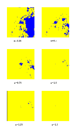
Refer to caption
Figure 1: A realization of the vacant set (dark blue) of RI(α\alpha) for different values of α\alpha. For α=1.5\alpha=1.5 the only vacant site is the origin. Also, note that we see the same neighbourhoods of the origin for α=1\alpha=1 and α=1.25\alpha=1.25; this is not surprising since just a few new walks enter the picture when increasing the rate by a small amount.

As a last step, we need to show that we have indeed constructed the object for which (2) is verified. For this, we need to prove the following fact:

Proposition 2.2.

For any finite set A⊂ℤ2A\subset{\mathbb{Z}}^{2} such that 0∈A0\in A it holds that cap(A)=cap^⁡(A)\mathop{\mathrm{cap}}(A)=\mathop{\widehat{\mathrm{cap}}}(A).

Proof.

Indeed, consider an arbitrary x∈∂Ax\in\partial A, x≠0x\neq 0, and (large) rr such that A⊂B⁡(r−2)A\subset B(r-2). Write using (6)

P^x[τ^1(A)>τ^1(∂B(r))]\displaystyle\widehat{P}_{x}\big[\widehat{\tau}_{1}(A)>\widehat{\tau}_{1}\big(\partial B(r)\big)\big] =∑ϱa⁡(ϱend)a⁡(x)​(14)|ϱ|\displaystyle=\sum_{\varrho}\frac{a(\varrho_{\text{end}})}{a(x)}\Big(\frac{1}{4}\Big)^{|\varrho|}
=(1+o⁡(1))​2π​ln⁡ra⁡(x)​∑ϱ(14)|ϱ|\displaystyle=\big(1+o(1)\big)\frac{\frac{2}{\pi}\ln r}{a(x)}\sum_{\varrho}\Big(\frac{1}{4}\Big)^{|\varrho|}
=(1+o(1))2π​ln⁡ra⁡(x)Px[τ1(A)>τ1(∂B(r))],\displaystyle=\big(1+o(1)\big)\frac{\frac{2}{\pi}\ln r}{a(x)}\,P_{x}\big[\tau_{1}(A)>\tau_{1}\big(\partial B(r)\big)\big],

where the sums are taken over all trajectories ϱ\varrho that start at xx, end at ∂B⁡(r)\partial B(r), and avoid A∪∂B⁡(r)A\cup\partial B(r) in between; ϱend∈∂B⁡(r)\varrho_{\text{end}}\in\partial B(r) stands for the ending point of the trajectory, and |ϱ||\varrho| is the trajectory’s length. Now, we send rr to infinity and use (10) to obtain that, if 0∈A0\in A,

a(x)P^x[τ^1(A)=∞]=hmA(x).a(x)\widehat{P}_{x}[\widehat{\tau}_{1}(A)=\infty]=\mathop{\mathrm{hm}}\nolimits_{A}(x). (15)

Multiplying by a⁡(x)a(x) and summing over x∈Ax\in A (recall that μx=a2​(x)\mu_{x}=a^{2}(x)) we obtain the expressions in (11) and (14) and thus conclude the proof. ∎

Together with formula (1.1) of [21], Proposition 2.2 shows the fundamental relation (2) announced in introduction: for all finite subsets AA of ℤ2{\mathbb{Z}}^{2} containing the origin,

ℙ[A⊂𝒱α]=exp(−παcap(A)).{\mathbb{P}}[A\subset{\mathcal{V}}^{\alpha}]=\exp\big(-\pi\alpha\mathop{\mathrm{cap}}(A)\big).

As mentioned before, the law of two-dimensional random interlacements is not translationally invariant, although it is of course invariant with respect to reflections/rotations of ℤ2{\mathbb{Z}}^{2} that preserve the origin. Let us describe some other basic properties of two-dimensional random interlacements:

Theorem 2.3.
  • (i)

    For any α>0\alpha>0, x∈ℤ2x\in{\mathbb{Z}}^{2}, A⊂ℤ2A\subset{\mathbb{Z}}^{2}, it holds that

    ℙ⁡[A⊂𝒱α∣x∈𝒱α]=ℙ⁡[−A+x⊂𝒱α∣x∈𝒱α].{\mathbb{P}}[A\subset{\mathcal{V}}^{\alpha}\mid x\in{\mathcal{V}}^{\alpha}]={\mathbb{P}}[-A+x\subset{\mathcal{V}}^{\alpha}\mid x\in{\mathcal{V}}^{\alpha}]. (16)

    More generally, for all α>0\alpha>0, x∈ℤ2∖{0}x\in{\mathbb{Z}}^{2}\setminus\{0\}, A⊂ℤ2A\subset{\mathbb{Z}}^{2}, and any lattice isometry MM exchanging 00 and xx, we have

    ℙ⁡[A⊂𝒱α∣x∈𝒱α]=ℙ⁡[M​A⊂𝒱α∣x∈𝒱α].{\mathbb{P}}[A\subset{\mathcal{V}}^{\alpha}\mid x\in{\mathcal{V}}^{\alpha}]={\mathbb{P}}[MA\subset{\mathcal{V}}^{\alpha}\mid x\in{\mathcal{V}}^{\alpha}]. (17)
  • (ii)

    With γ′\gamma^{\prime} from (6) we have

    ℙ[x∈𝒱α]=exp(−παa⁡(x)2)=e−γ′πα/2∥x∥−α(1+O(∥x∥−2)).{\mathbb{P}}[x\in{\mathcal{V}}^{\alpha}]=\exp\Big(-\pi\alpha\frac{a(x)}{2}\Big)=e^{-\gamma^{\prime}\pi\alpha/2}\|x\|^{-\alpha}\big(1+O(\|x\|^{-2})\big). (18)
  • (iii)

    For AA such that 0∈A⊂B⁡(r)0\in A\subset B(r) and x∈ℤ2x\in{\mathbb{Z}}^{2} such that ‖x‖≥2​r\|x\|\geq 2r we have

    ℙ[A⊂𝒱α∣x∈𝒱α]=exp(−π​α4cap(A)1+O⁡(r​ln⁡r​ln⁡‖x‖‖x‖)1−cap(A)2​a​(x)+O⁡(r​ln⁡r‖x‖)).{\mathbb{P}}[A\subset{\mathcal{V}}^{\alpha}\mid x\in{\mathcal{V}}^{\alpha}]=\exp\Bigg(-\frac{\pi\alpha}{4}\mathop{\mathrm{cap}}(A)\frac{1+O\big(\frac{r\ln r\ln\|x\|}{\|x\|}\big)}{1-\frac{\mathop{\mathrm{cap}}(A)}{2a(x)}+O\big(\frac{r\ln r}{\|x\|}\big)}\Bigg). (19)
  • (iv)

    For x,y≠0x,y\neq 0, x≠yx\neq y, we have ℙ[{x,y}⊂𝒱α]=exp(−παΨ){\mathbb{P}}\big[\{x,y\}\subset{\mathcal{V}}^{\alpha}\big]=\exp\big(-\pi\alpha\Psi\big), where

    Ψ=a⁡(x)​a​(y)​a​(x−y)a⁡(x)​a​(y)+a⁡(x)​a​(x−y)+a⁡(y)​a​(x−y)−12​(a2​(x)+a2​(y)+a2​(x−y)).\Psi=\frac{a(x)a(y)a(x-y)}{a(x)a(y)+a(x)a(x-y)+a(y)a(x-y)-\frac{1}{2}\big(a^{2}(x)+a^{2}(y)+a^{2}(x-y)\big)}.

    Moreover, as s:=‖x‖→∞s:=\|x\|\to\infty, ln⁡‖y‖∼ln⁡s\ln\|y\|\sim\ln s and ln⁡‖x−y‖∼β​ln⁡s\ln\|x-y\|\sim\beta\ln s with some β∈[0,1]\beta\in[0,1], we have

    ℙ[{x,y}⊂𝒱α]=s−4​α4−β+o⁡(1),{\mathbb{P}}\big[\{x,y\}\subset{\mathcal{V}}^{\alpha}\big]=s^{-\frac{4\alpha}{4-\beta}+o(1)},

    and polynomially decaying correlations (cf. (3) in Remark 2.4 for the definition),

    Cor({x∈𝒱α},{y∈𝒱α})=s−α​β4−β+o⁡(1).\mathop{\mathrm{Cor}}\big({\{x\in{\mathcal{V}}^{\alpha}\}},{\{y\in{\mathcal{V}}^{\alpha}\}}\big)=s^{-\frac{\alpha\beta}{4-\beta}+o(1)}. (20)
  • (v)

    Assume that ln⁡‖x‖∼ln⁡s\ln\|x\|\sim\ln s, ln⁡r∼β​ln⁡s\ln r\sim\beta\ln s with β<1\beta<1. Then, as s→∞s\to{\infty},

    ℙ[B(x,r)⊂𝒱α]=s−2​α2−β+o⁡(1).{\mathbb{P}}\big[B(x,r)\subset{\mathcal{V}}^{\alpha}\big]=s^{-\frac{2\alpha}{2-\beta}+o(1)}. (21)

These results invite a few comments.

Remark 2.4.
  1. 1.

    The statement in (i) describes an invariance property given that a point is vacant. We refer to it as the conditional stationarity

  2. 2.

    We can interpret (iii) as follows: the conditional law of RI(α\alpha) given that a distant site xx is vacant, is similar – near the origin – to the unconditional law of RI(α/4\alpha/4). Combined with (i), the similarity holds near xx as well. Moreover, one can also estimate the “local rate” away from the origin, see Figure 2. More specifically, observe from Lemma 3.9 (ii) that cap(A2)≪ln⁡s\mathop{\mathrm{cap}}(A_{2})\ll\ln s with s=dist⁡(0,A2)s={\rm dist}(0,A_{2}) large implies cap({0}∪A2)=a⁡(s)2​(1+o⁡(1))\mathop{\mathrm{cap}}\big(\{0\}\cup A_{2}\big)=\frac{a(s)}{2}(1+o(1)). If xx is at a much larger distance from the origin than A2A_{2}, say ln⁡‖x‖∼ln⁡(s2)\ln\|x\|\sim\ln(s^{2}), then (19) reveals a “local rate” equal to 27​α\frac{2}{7}\alpha, that is, ℙ[A2⊂𝒱α∣x∈𝒱α]=exp(−27παcap({0}∪A2)(1+o(1))){\mathbb{P}}[A_{2}\subset{\mathcal{V}}^{\alpha}\mid x\in{\mathcal{V}}^{\alpha}]=\exp\big(-\frac{2}{7}\pi\alpha\mathop{\mathrm{cap}}\big(\{0\}\cup A_{2}\big)(1+o(1))\big); indeed, the expression in the denominator in (19) equals approximately 1−cap({0}∪A2)2​a​(x)≈1−a⁡(s)/22​a​(s2)≈781-\frac{\mathop{\mathrm{cap}}(\{0\}\cup A_{2})}{2a(x)}\approx 1-\frac{a(s)/2}{2a(s^{2})}\approx\frac{7}{8}.

  3. 3.

    Recall that the correlation between two events AA and BB,

    Cor(A,B)=Cov⁡(𝟏A,𝟏B)[Var(𝟏A)​Var(𝟏B)]1/2∈[−1,1],\mathop{\mathrm{Cor}}(A,B)=\frac{{\rm Cov}({\mathbf{1}}_{A},{\mathbf{1}}_{B})}{[\mathop{\mathrm{Var}}({\mathbf{1}}_{A})\mathop{\mathrm{Var}}({\mathbf{1}}_{B})]^{1/2}}\in[-1,1],

    can be viewed as the cosine of the angle between the vectors 𝟏A−ℙ⁡(A),𝟏B−ℙ⁡(B){\mathbf{1}}_{A}-{\mathbb{P}}(A),{\mathbf{1}}_{B}-{\mathbb{P}}(B) in the corresponding Hilbert space L2L^{2}. Then, equation (20) relates the geometry of the lattice with the geometry of the random point process: For points xx and yy at large distance ss making a small angle s1−βs^{1-\beta} with the origin, the random variables 𝟏{x∈𝒱α}{\mathbf{1}}{\{x\in{\mathcal{V}}^{\alpha}\}} and 𝟏{y∈𝒱α}{\mathbf{1}}{\{y\in{\mathcal{V}}^{\alpha}\}} make, after centering, an angle of order s−α​β4−βs^{-\frac{\alpha\beta}{4-\beta}} in the space of square integrable random variables.

  4. 4.

    By symmetry, the conclusion of (iv) remains the same in the situation when ln⁡‖x‖,ln⁡‖x−y‖∼ln⁡s\ln\|x\|,\ln\|x-y\|\sim\ln s and ln⁡‖y‖∼β​ln⁡s\ln\|y\|\sim\beta\ln s.

Refer to caption
Figure 2: How the “local rate” looks like if we condition on the event that a “distant” site is vacant.
Proof of (i) and (ii).

To prove (i), observe that

cap({0,x}∪A)=cap({0,x}∪(−A+x))\mathop{\mathrm{cap}}\big(\{0,x\}\cup A\big)=\mathop{\mathrm{cap}}\big(\{0,x\}\cup(-A+x)\big)

by symmetry. For the second statement in (i), note that, for A′={0,x}∪AA^{\prime}=\{0,x\}\cup A, it holds that cap(A′)=cap(M​A′)=cap({0,x}∪M​A).\mathop{\mathrm{cap}}\big(A^{\prime}\big)=\mathop{\mathrm{cap}}\big(MA^{\prime}\big)=\mathop{\mathrm{cap}}\big(\{0,x\}\cup MA\big). Item (ii) follows from the above mentioned fact that cap({0,x})=12​a​(x)\mathop{\mathrm{cap}}\big(\{0,x\}\big)=\frac{1}{2}a(x) together with (6). ∎

We postpone the proof of other parts of Theorem 2.3, since it requires some estimates for capacities of various kinds of sets. We now turn to estimates on the cardinality of the vacant set.

Theorem 2.5.
  • (i)

    We have

    𝔼⁡(|𝒱α∩B⁡(r)|)∼{2​π2−αe−γ′πα/2×r2−α, for ​α<2,2πe−γ′πα/2×lnr, for ​α=2,const, for ​α>2.{\mathbb{E}}\big(|{\mathcal{V}}^{\alpha}\cap B(r)|\big)\sim\begin{cases}\frac{2\pi}{2-\alpha}e^{-\gamma^{\prime}\pi\alpha/2}\times r^{2-\alpha},&\text{ for }\alpha<2,\\ 2\pi e^{-\gamma^{\prime}\pi\alpha/2}\times\ln r,&\text{ for }\alpha=2,\\ \text{const},&\text{ for }\alpha>2.\end{cases}
  • (ii)

    For α>1\alpha>1 it holds that 𝒱α{\mathcal{V}}^{\alpha} is finite a.s. Moreover, ℙ[𝒱α={0}]>0{\mathbb{P}}\big[{\mathcal{V}}^{\alpha}=\{0\}\big]>0 and ℙ[𝒱α={0}]→1{\mathbb{P}}\big[{\mathcal{V}}^{\alpha}=\{0\}\big]\to 1 as α→∞\alpha\to\infty.

  • (iii)

    For α∈(0,1)\alpha\in(0,1), we have |𝒱α|=∞|{\mathcal{V}}^{\alpha}|=\infty a.s. Moreover,

    ℙ[𝒱α∩(B(r)∖B(r/2))=∅]≤r−2​(1−α)2+o⁡(1).{\mathbb{P}}\big[{\mathcal{V}}^{\alpha}\cap\big(B(r)\setminus B(r/2)\big)=\emptyset\big]\leq r^{-2(1-\sqrt{\alpha})^{2}+o(1)}. (22)

It is worth noting that the “phase transition” at α=1\alpha=1 in (ii) corresponds to the cover time of the torus, as shown in Theorem 2.6 below.

Proof of (i) and (ii) (incomplete, in the latter case).

Part (i) immediately follows from Theorem 2.3 (ii).

The proof of the part (ii) is easy in the case α>2\alpha>2. Indeed, observe first that 𝔼​|𝒱α|<∞{\mathbb{E}}|{\mathcal{V}}^{\alpha}|<\infty implies that 𝒱α{\mathcal{V}}^{\alpha} itself is a.s. finite. Also, Theorem 2.3 (ii) actually implies that 𝔼​|𝒱α∖{0}|→0{\mathbb{E}}|{\mathcal{V}}^{\alpha}\setminus\{0\}|\to 0 as α→∞\alpha\to\infty, so ℙ[𝒱α={0}]→1{\mathbb{P}}\big[{\mathcal{V}}^{\alpha}=\{0\}\big]\to 1 by the Chebyshev inequality.

Now, let us prove that, in general, ℙ[|𝒱α|<∞]=1{\mathbb{P}}\big[|{\mathcal{V}}^{\alpha}|<\infty\big]=1 implies that ℙ[𝒱α={0}]>0{\mathbb{P}}\big[{\mathcal{V}}^{\alpha}=\{0\}\big]>0. Indeed, if 𝒱α{\mathcal{V}}^{\alpha} is a.s. finite, then one can find a sufficiently large RR such that ℙ[|𝒱α∩(ℤ2∖B(R))|=0]>0{\mathbb{P}}\big[|{\mathcal{V}}^{\alpha}\cap({\mathbb{Z}}^{2}\setminus B(R))|=0\big]>0. Since ℙ[x∉𝒱α]>0{\mathbb{P}}[x\notin{\mathcal{V}}^{\alpha}]>0 for any x≠0x\neq 0, the claim that ℙ[𝒱α={0}]>0{\mathbb{P}}\big[{\mathcal{V}}^{\alpha}=\{0\}\big]>0 follows from the FKG inequality applied to events {x∉𝒱α}\{x\notin{\mathcal{V}}^{\alpha}\}, x∈B⁡(R)x\in B(R) together with {|𝒱α∩(ℤ2∖B(R))|=0}\big\{|{\mathcal{V}}^{\alpha}\cap({\mathbb{Z}}^{2}\setminus B(R))|=0\big\}. ∎

As before, we postpone the proof of part (iii) and the rest of part (ii) of Theorem 2.5. Let us remark that we believe that the right-hand side of (22) gives the correct order of decay of the above probability; we, however, do not have a rigorous argument at the moment. Also, note that the question whether 𝒱1{\mathcal{V}}^{1} is a.s. finite or not, is open.

Let us now give a heuristic explanation about the unusual behaviour of the model for α∈(1,2)\alpha\in(1,2): in this non-trivial interval, the vacant set is a.s. finite but its expected size is infinite. The reason is the following: the number of S^{\widehat{S}}-walks that hit B⁡(r)B(r) has Poisson law with rate of order ln⁡r\ln r (recall (12)). Thus, decreasing this number by a constant factor (with respect to the expectation) has only a polynomial cost. On the other hand, by doing so, we increase the probability that a site x∈B⁡(r)x\in B(r) is vacant for all x∈B⁡(r)x\in B(r) at once, which increases the expected size of 𝒱α∩B⁡(r){\mathcal{V}}^{\alpha}\cap B(r) by a polynomial factor. It turns out that this effect causes the actual number of uncovered sites in B⁡(r)B(r) to be typically of much smaller order then the expected number of uncovered sites there.

2.2 Simple random walk on a discrete torus and its relationship with random interlacements

Now, we state our results for random walk on the torus. Let (Xk,k≥0)(X_{k},k\geq 0) be simple random walk on ℤn2{\mathbb{Z}}^{2}_{n} with X0X_{0} chosen uniformly at random. Define the entrance time to the site x∈ℤn2x\in{\mathbb{Z}}^{2}_{n} by

Tn​(x)=inf{t≥0:Xt=x},T_{n}(x)=\inf\{t\geq 0:X_{t}=x\}, (23)

and the cover time of the torus by

𝒯n=maxx∈ℤn2⁡Tn​(x).{\mathcal{T}}_{n}=\max_{x\in{\mathbb{Z}}^{2}_{n}}T_{n}(x). (24)

Let us also define the uncovered set at time tt,

Ut(n)={x∈ℤn2:Tn​(x)>t}.U_{t}^{(n)}=\{x\in{\mathbb{Z}}^{2}_{n}:T_{n}(x)>t\}. (25)

Denote by Υn:ℤ2→ℤn2\Upsilon_{n}:{\mathbb{Z}}^{2}\to{\mathbb{Z}}^{2}_{n}, Υn​(x,y)=(xmodn,ymodn)\Upsilon_{n}(x,y)=(x\mod n,y\mod n), the natural projection modulo nn. Then, if S0S_{0} were chosen uniformly at random on any fixed n×nn\times n square, we can write Xk=Υn​(Sk)X_{k}=\Upsilon_{n}(S_{k}). Similarly, B⁡(y,r)⊂ℤn2B(y,r)\subset{\mathbb{Z}}^{2}_{n} is defined by B⁡(y,r)=Υn​B​(z,r)B(y,r)=\Upsilon_{n}B(z,r), where z∈ℤ2z\in{\mathbb{Z}}^{2} is such that Υn​z=y\Upsilon_{n}z=y. Let also

tα:=4​απ​n2​ln2​nt_{\alpha}:=\frac{4\alpha}{\pi}n^{2}\ln^{2}n

(recall that, as mentioned in Section 1.2, α=1\alpha=1 corresponds to the leading-order term of the expected cover time of the torus). In the following theorem, we prove that, given that 00 is uncovered, the law of the uncovered set around 00 at time tαt_{\alpha} is close to that of RI(α\alpha):

Theorem 2.6.

Let α>0\alpha>0 and AA be a finite subset of ℤ2{\mathbb{Z}}^{2} such that 0∈A0\in A. Then, we have

limn→∞ℙ[ΥnA⊂Utα(n)∣0∈Utα(n)]=exp(−παcap(A)).\lim_{n\to\infty}{\mathbb{P}}[\Upsilon_{n}A\subset U_{t_{\alpha}}^{(n)}\mid 0\in U_{t_{\alpha}}^{(n)}]=\exp\big(-\pi\alpha\mathop{\mathrm{cap}}(A)\big). (26)

Let us also mention that, for higher dimensions, results similar to the above theorem have appeared in the literature, see Theorem 0.1 of [19] and Theorem 1.1 of [23]. Also, stronger “coupling” results are available, see e.g. [1, 5, 18, 22].

The proof of this theorem will be presented in Section 4.

Refer to caption
Figure 3: Excursions (depicted as the solid pieces of the trajectory) of the SRW on the torus ℤn2{\mathbb{Z}}^{2}_{n}

To give a brief heuristic explanation for (26), consider the excursions of the random walk XX between ∂B⁡(n3​ln⁡n)\partial B\big(\frac{n}{3\ln n}\big) and ∂B⁡(n/3)\partial B(n/3) up to time tαt_{\alpha}. We hope that Figure 3 is self-explanatory; formal definitions are presented in Section 3.4. It is possible to prove that the number of these excursions is concentrated around N=2​α​ln2⁡nln⁡ln⁡nN=\frac{2\alpha\ln^{2}n}{\ln\ln n}. Also, one can show that each excursion hits a finite set AA (such that 0∈A0\in A) approximately independently of the others (also when conditioning on 0∈Utα(n)0\in U_{t_{\alpha}}^{(n)}), with probability roughly equal to p=π​ln⁡ln​n2​ln2​n​cap(A)p=\frac{\pi\ln\ln n}{2\ln^{2}n}\mathop{\mathrm{cap}}(A). This heuristically gives (26) since (1−p)N≈exp(−παcap(A))(1-p)^{N}\approx\exp\big(-\pi\alpha\mathop{\mathrm{cap}}(A)\big).

3 Some auxiliary facts and estimates

In this section we collect lemmas of all sorts that will be needed in the sequel.

3.1 Simple random walk in ℤ2{\mathbb{Z}}^{2}

First, we recall a couple of basic facts for the exit probabilities of simple random walk.

Lemma 3.1.

For all x,y∈ℤ2x,y\in{\mathbb{Z}}^{2} and R>0R>0 with x∈B⁡(y,R),‖y‖≤R−2x\in B(y,R),\|y\|\leq R-2, we have

Px[τ1(0)>τ1(∂B(y,R))]=a⁡(x)a⁡(R)+O⁡(‖y‖∨1R),P_{x}\big[\tau_{1}(0)>\tau_{1}\big(\partial B(y,R)\big)\big]=\frac{a(x)}{a(R)+O\big(\frac{\|y\|\vee 1}{R}\big)}\;, (27)

and for all y∈B⁡(r),x∈B⁡(y,R)∖B⁡(r)y\in B(r),x\in B(y,R)\setminus B(r) with r+‖y‖≤R−2r+\|y\|\leq R-2, we have

Px[τ1(∂B(r))>τ1(∂B(y,R))]=a⁡(x)−a⁡(r)+O⁡(r−1)a⁡(R)−a⁡(r)+O⁡(‖y‖∨1R+r−1),P_{x}\big[\tau_{1}(\partial B(r))>\tau_{1}\big(\partial B(y,R)\big)\big]=\frac{a(x)-a(r)+O(r^{-1})}{a(R)-a(r)+O\big(\frac{\|y\|\vee 1}{R}+r^{-1}\big)}\;, (28)

as r,R→∞r,R\to\infty.

Proof.

Both (27) and (28) are easily deduced from the following argument: recall that the sequence a⁡(Sk∧τ0​(0)),k≥0,a(S_{k\wedge\tau_{0}(0)}),k\geq 0, is a martingale, and apply the Optional Stopping Theorem together with (6) and (8). For the second statement, with

τ=τ1(∂B(r))∧τ1(∂B(y,R)) and q=Px[τ1(∂B(r))>τ1(∂B(y,R))],\tau=\tau_{1}(\partial B(r))\wedge\tau_{1}\big(\partial B(y,R)\big)\quad\text{ and }\quad q=P_{x}\big[\tau_{1}(\partial B(r))>\tau_{1}\big(\partial B(y,R)\big)\big],

we write

a⁡(x)\displaystyle a(x) =Ex​[a⁡(Sτ);τ=τ1​(∂B⁡(y,R))]+Ex​[a⁡(Sτ);τ=τ1​(∂B⁡(r))]\displaystyle=E_{x}\big[a(S_{\tau});\tau=\tau_{1}(\partial B(y,R))\big]+E_{x}\big[a(S_{\tau});\tau=\tau_{1}(\partial B(r))\big]
=q⁡(a⁡(R)+O⁡(‖y‖∨1R))+(1−q)​(a⁡(r)+O⁡(r−1)),\displaystyle=q\big(a(R)+O\big(\textstyle\frac{\|y\|\vee 1}{R}\big)\big)+(1-q)\big(a(r)+O(r^{-1})\big),

yielding (28). The first statement has a similar proof. ∎

We have an estimate for more general sets.

Lemma 3.2.

Let AA be a finite subset of ℤ2{\mathbb{Z}}^{2} such that A⊂B⁡(r)A\subset B(r) for some r>0r>0. We have for r+1≤‖x‖≤R−2r+1\leq\|x\|\leq R-2, ‖x‖+‖y‖≤R−1\|x\|+\|y\|\leq R-1

Px[τ1(A)>τ1(∂B(y,R))]=a⁡(x)−cap(A)+O⁡(r​ln⁡r​ln⁡‖x‖‖x‖)a⁡(R)−cap(A)+O⁡(‖y‖∨1R+r​ln⁡r​ln⁡‖x‖‖x‖).P_{x}\big[\tau_{1}(A)>\tau_{1}\big(\partial B(y,R)\big)\big]=\frac{a(x)-\mathop{\mathrm{cap}}(A)+O\big(\frac{r\ln r\ln\|x\|}{\|x\|}\big)}{a(R)-\mathop{\mathrm{cap}}(A)+O\big(\frac{\|y\|\vee 1}{R}+\frac{r\ln r\ln\|x\|}{\|x\|}\big)}. (29)
Proof.

First, observe that, for u∈Au\in A,

Px[Sτ1​(A)=u]=hmA(u)(1+O(r​ln⁡‖x‖‖x‖)).P_{x}\big[S_{\tau_{1}(A)}=u\big]=\mathop{\mathrm{hm}}\nolimits_{A}(u)\big(1+O\big(\textstyle\frac{r\ln\|x\|}{\|x\|}\big)\big). (30)

Indeed, from (6.42) and the last display on page 178 of [13] we obtain

Px[Sτ1​(A)=u]Px′[Sτ1​(A)=u]=1+O⁡(r​ln⁡‖x‖‖x‖)\frac{P_{x}\big[S_{\tau_{1}(A)}=u\big]}{P_{x^{\prime}}\big[S_{\tau_{1}(A)}=u\big]}=1+O\big(\textstyle\frac{r\ln\|x\|}{\|x\|}\big)

for all x′∈∂B⁡(‖x‖)x^{\prime}\in\partial B(\|x\|). Since hmA(u)\mathop{\mathrm{hm}}\nolimits_{A}(u) is a linear combination of Px′[Sτ1​(A)=u]P_{x^{\prime}}\big[S_{\tau_{1}(A)}=u\big], x′∈∂B⁡(‖x‖)x^{\prime}\in\partial B(\|x\|), (30) follows.

Then, we can write

Px​[Sτ1​(A)=u,τ1​(A)<τ1​(∂B⁡(y,R))]\displaystyle P_{x}\big[S_{\tau_{1}(A)}=u,\tau_{1}(A)<\tau_{1}\big(\partial B(y,R)\big)\big]
=Px[Sτ1​(A)=u]−Px[Sτ1​(A)=u,τ1(A)>τ1(∂B(y,R))]\displaystyle=P_{x}\big[S_{\tau_{1}(A)}=u\big]-P_{x}\big[S_{\tau_{1}(A)}=u,\tau_{1}(A)>\tau_{1}\big(\partial B(y,R)\big)\big]
=hmA(u)(1+O(r​ln⁡‖x‖‖x‖))−Px[τ1(A)>τ1(∂B(y,R))]\displaystyle=\mathop{\mathrm{hm}}\nolimits_{A}(u)\big(1+O\big(\textstyle\frac{r\ln\|x\|}{\|x\|}\big)\big)-P_{x}\big[\tau_{1}(A)>\tau_{1}\big(\partial B(y,R)\big)\big]
×∑z∈∂B⁡(y,R)Pz[Sτ1​(A)=u]Px[Sτ1​(∂B⁡(y,R))=z∣τ1(A)>τ1(∂B(y,R))]\displaystyle\qquad\times\sum_{z\in\partial B(y,R)}P_{z}\big[S_{\tau_{1}(A)}=u\big]P_{x}\big[S_{\tau_{1}(\partial B(y,R))}=z\mid\tau_{1}(A)>\tau_{1}\big(\partial B(y,R)\big)\big]
=hmA(u)(1+O(r​ln⁡‖x‖‖x‖))−Px[τ1(A)>τ1(∂B(y,R))]hmA(u)(1+O(r​ln⁡RR))\displaystyle=\mathop{\mathrm{hm}}\nolimits_{A}(u)\big(1+O\big(\textstyle\frac{r\ln\|x\|}{\|x\|}\big)\big)-P_{x}\big[\tau_{1}(A)>\tau_{1}\big(\partial B(y,R)\big)\big]\mathop{\mathrm{hm}}\nolimits_{A}(u)\big(1+O\big(\textstyle\frac{r\ln R}{R}\big)\big)
=hmA(u)Px[τ1(A)<τ1(∂B(y,R))](1+O(r​ln⁡‖x‖‖x‖)),\displaystyle=\mathop{\mathrm{hm}}\nolimits_{A}(u)P_{x}\big[\tau_{1}(A)<\tau_{1}\big(\partial B(y,R)\big)\big]\big(1+O\big(\textstyle\frac{r\ln\|x\|}{\|x\|}\big)\big),

using twice the above observation and also that B⁡(‖x‖)⊂B⁡(y,R)B(\|x\|)\subset B(y,R), yielding

Px​[Sτ1​(A)=u∣τ1​(A)<τ1​(∂B⁡(y,R))]=hmA(u)​(1+O⁡(r​ln⁡‖x‖‖x‖)).P_{x}\big[S_{\tau_{1}(A)}=u\mid\tau_{1}(A)<\tau_{1}\big(\partial B(y,R)\big)\big]=\mathop{\mathrm{hm}}\nolimits_{A}(u)\big(1+O\big(\textstyle\frac{r\ln\|x\|}{\|x\|}\big)\big). (31)

Abbreviating q:=Px[τ1(A)>τ1(∂B(y,R))]q:=P_{x}\big[\tau_{1}(A)>\tau_{1}\big(\partial B(y,R)\big)\big], we have by the Optional Stopping Theorem and (31)

a⁡(x)\displaystyle a(x) =q⁡(a⁡(R)+O⁡(‖y‖∨1R))+(1−q)​∑u∈A∖{0}a⁡(u)​hmA(u)​(1+O⁡(r​ln⁡‖x‖‖x‖))\displaystyle=q\big(a(R)+O\big(\textstyle\frac{\|y\|\vee 1}{R}\big)\big)+(1-q)\sum_{u\in A\setminus\{0\}}a(u)\mathop{\mathrm{hm}}\nolimits_{A}(u)\big(1+O\big(\textstyle\frac{r\ln\|x\|}{\|x\|}\big)\big)
=q⁡(a⁡(R)+O⁡(‖y‖∨1R))+(1−q)​(1+O⁡(r​ln⁡‖x‖‖x‖))​cap(A),\displaystyle=q\big(a(R)+O\big(\textstyle\frac{\|y\|\vee 1}{R}\big)\big)+(1-q)\big(1+O\big(\textstyle\frac{r\ln\|x\|}{\|x\|}\big)\big)\mathop{\mathrm{cap}}(A),

and (29) follows (observe also that cap(A)≤cap(B⁡(r))=2π​ln⁡r+O⁡(1)\mathop{\mathrm{cap}}(A)\leq\mathop{\mathrm{cap}}(B(r))=\frac{2}{\pi}\ln r+O(1), see (12)). ∎

3.2 Simple random walk conditioned on not hitting the origin

Next, we relate the probabilities of certain events for the walks SS and S^{\widehat{S}}. For M⊂ℤ2M\subset{\mathbb{Z}}^{2}, let ΓM(x)\Gamma^{(x)}_{M} be the set of all nearest-neighbour finite trajectories that start at x∈M∖{0}x\in M\setminus\{0\} and end when entering ∂M\partial M for the first time; denote also Γy,R(x)=ΓB⁡(y,R)(x)\Gamma^{(x)}_{y,R}=\Gamma^{(x)}_{B(y,R)}. For A⊂ΓM(x)A\subset\Gamma^{(x)}_{M} write S∈AS\in A if there exists kk such that (S0,…,Sk)∈A(S_{0},\ldots,S_{k})\in A (and the same for the conditional walk S^{\widehat{S}}). In the next result we show that Px[⋅∣τ1(0)>τ1(∂B(R))]P_{x}\big[\;\cdot\mid\tau_{1}(0)>\tau_{1}\big(\partial B(R)\big)\big] and P^x​[⋅]\widehat{P}_{x}[\,\cdot\,] are almost indistinguishable on Γ0,R(x)\Gamma^{(x)}_{0,R} (that is, the conditional law of SS almost coincides with the unconditional law of S^{\widehat{S}}). A similar result holds for excursions on a “distant” (from the origin) set.

Lemma 3.3.
  • (i)

    Assume A⊂Γ0,R(x)A\subset\Gamma^{(x)}_{0,R}. We have

    Px[S∈A∣τ1(0)>τ1(∂B(R))]=P^x[S^∈A](1+O((RlnR)−1)).P_{x}\big[S\in A\mid\tau_{1}(0)>\tau_{1}\big(\partial B(R)\big)\big]=\widehat{P}_{x}\big[{\widehat{S}}\in A\big]\big(1+O((R\ln R)^{-1})\big). (32)
  • (ii)

    Assume that A⊂ΓM(x)A\subset\Gamma^{(x)}_{M} and suppose that 0∉M0\notin M, and denote s=dist(0,M)s=\mathop{\mathrm{dist}}(0,M), r=diam(M)r={\mathop{\mathrm{diam}}}(M). Then, for x∈Mx\in M,

    Px[S∈A]=P^x[S^∈A](1+O(rs​ln⁡s)).P_{x}[S\in A]=\widehat{P}_{x}[{\widehat{S}}\in A]\Big(1+O\Big(\frac{r}{s\ln s}\Big)\Big). (33)
Proof.

Let us prove part (i). Assume without loss of generality that no trajectory from AA passes through the origin. Then, it holds that

P^x[S^∈A]=∑ϱ∈Aa⁡(ϱend)a⁡(x)(14)|ϱ|,\widehat{P}_{x}[{\widehat{S}}\in A]=\sum_{\varrho\in A}\frac{a(\varrho_{\text{end}})}{a(x)}\Big(\frac{1}{4}\Big)^{|\varrho|},

with |ϱ||\varrho| the length of ϱ\varrho. On the other hand, by (27)

Px​[S∈A∣τ1​(0)>τ1​(∂B⁡(R))]=a⁡(R)+O⁡(R−1)a⁡(x)​∑ϱ∈A(14)|ϱ|.P_{x}[S\in A\mid\tau_{1}(0)>\tau_{1}\big(\partial B(R)\big)]=\frac{a(R)+O(R^{-1})}{a(x)}\sum_{\varrho\in A}\Big(\frac{1}{4}\Big)^{|\varrho|}.

Since ϱend∈∂B⁡(R)\varrho_{\text{end}}\in\partial B(R), we have a⁡(ϱend)=a⁡(R)+O⁡(R−1)a(\varrho_{\text{end}})=a(R)+O(R^{-1}), and so (32) follows.

The proof of part (ii) is analogous (observe that a⁡(y1)/a⁡(y2)=1+O⁡(rs​ln⁡s)a(y_{1})/a(y_{2})=1+O\big(\frac{r}{s\ln s}\big) for any y1,y2∈My_{1},y_{2}\in M). ∎

As observed in Section 1.1, the random walk S^{\widehat{S}} is transient. Next, we estimate the probability that the S^{\widehat{S}}-walk avoids a ball centered at the origin:

Lemma 3.4.

Assume r≥1r\geq 1 and ‖x‖≥r+1\|x\|\geq r+1. We have

P^x[τ^1(B(r))=∞]=1−a⁡(r)+O⁡(r−1)a⁡(x).\widehat{P}_{x}\big[\widehat{\tau}_{1}\big(B(r)\big)=\infty\big]=1-\frac{a(r)+O(r^{-1})}{a(x)}.
Proof.

By Lemma 3.3 (i) we have

P^x[τ^1(B(r))=∞]=limR→∞Px[τ1(∂B(r))>τ1(∂B(R))∣τ1(0)>τ1(∂B(R))].\widehat{P}_{x}\big[\widehat{\tau}_{1}\big(B(r)\big)=\infty\big]=\lim_{R\to\infty}P_{x}\big[\tau_{1}(\partial B(r))>\tau_{1}\big(\partial B(R)\big)\mid\tau_{1}(0)>\tau_{1}\big(\partial B(R)\big)\big].

The claim then follows from (27)–(28). ∎

Remark 3.5.

Alternatively, one can deduce the proof of Lemma 3.4 from the fact that 1/a⁡(S^k∧τ^0​(𝒩))1/a({\widehat{S}}_{k\wedge\widehat{\tau}_{0}(\mathcal{N})}) is a martingale, together with the Optional Stopping Theorem.

We will need also an expression for the probability of avoiding any finite set containing the origin:

Lemma 3.6.

Assume that 0∈A⊂B⁡(r)0\in A\subset B(r), and ‖x‖≥r+1\|x\|\geq r+1. Then

P^x[τ^1(A)=∞]=1−cap(A)a⁡(x)+O(r​ln⁡r​ln⁡‖x‖‖x‖).\widehat{P}_{x}[\widehat{\tau}_{1}(A)=\infty]=1-\frac{\mathop{\mathrm{cap}}(A)}{a(x)}+O\Big(\frac{r\ln r\ln\|x\|}{\|x\|}\Big). (34)
Proof.

Indeed, using Lemmas 3.2 and 3.3 (i) together with (27), we write

P^x[τ^1(A)=∞]\displaystyle\widehat{P}_{x}[\widehat{\tau}_{1}(A)=\infty] =limR→∞Px​[τ1​(A)>τ1​(∂B⁡(R))∣τ1​(0)>τ1​(∂B⁡(R))]\displaystyle=\lim_{R\to\infty}P_{x}\big[\tau_{1}(A)>\tau_{1}\big(\partial B(R)\big)\mid\tau_{1}(0)>\tau_{1}\big(\partial B(R)\big)\big]
=limR→∞a⁡(R)+O⁡(R−1)a⁡(x)×a⁡(x)−cap(A)+O⁡(r​ln⁡r​ln⁡‖x‖‖x‖)a⁡(R)−cap(A)+O⁡(R−1+r​ln⁡r​ln⁡‖x‖‖x‖),\displaystyle=\lim_{R\to\infty}\frac{a(R)+O(R^{-1})}{a(x)}\times\frac{a(x)-\mathop{\mathrm{cap}}(A)+O\big(\frac{r\ln r\ln\|x\|}{\|x\|}\big)}{a(R)-\mathop{\mathrm{cap}}(A)+O\big(R^{-1}+\frac{r\ln r\ln\|x\|}{\|x\|}\big)},

thus obtaining (34). ∎

It is also possible to obtain exact expressions for one-site escape probabilities, and probabilities of (not) hitting a given site:

P^x[τ^1(y)<∞]\displaystyle\widehat{P}_{x}[\widehat{\tau}_{1}(y)<\infty] =a⁡(x)+a⁡(y)−a⁡(x−y)2​a​(x),\displaystyle=\frac{a(x)+a(y)-a(x-y)}{2a(x)}, (35)
for x≠yx\neq y, x,y≠0x,y\neq 0 and
P^x[τ^1(x)<∞]\displaystyle\widehat{P}_{x}[\widehat{\tau}_{1}(x)<\infty] =1−12​a​(x)\displaystyle=1-\frac{1}{2a(x)} (36)

for x≠0x\neq 0. We temporarily postpone the proof of (35)–(36). Observe that, in particular, we recover from (36) the transience of S^{\widehat{S}}. Also, observe that (35) implies the following surprising fact: for any x≠0x\neq 0,

limy→∞P^x[τ^1(y)<∞]=12.\lim_{y\to\infty}\widehat{P}_{x}[\widehat{\tau}_{1}(y)<\infty]=\frac{1}{2}.

The above relation leads to the following heuristic explanation for Theorem 2.3 (iii) (in the case when AA is fixed and ‖x‖→∞\|x\|\to{\infty}). Since the probability of hitting a distant site is about 1/21/2, by conditioning that this distant site is vacant, we essentially throw away three quarters of the trajectories that pass through a neighbourhood of the origin: indeed, the double-infinite trajectory has to avoid this distant site two times, before and after reaching that neighbourhood.

Let us state several other general estimates, for the probability of (not) hitting a given set (which is, typically, far away from the origin), or, more specifically, a disk:

Lemma 3.7.

Assume that x∉B⁡(y,r)x\notin B(y,r) and ‖y‖>2​r≥1\|y\|>2r\geq 1. Abbreviate also Ψ1=‖y‖−1​r\Psi_{1}=\|y\|^{-1}r, Ψ2=r​ln⁡r​ln⁡‖y‖‖y‖\Psi_{2}=\frac{r\ln r\ln\|y\|}{\|y\|}, Ψ3=r​ln⁡r⁡(ln⁡‖x−y‖‖x−y‖+ln⁡‖y‖‖y‖)\Psi_{3}=r\ln r\big(\frac{\ln\|x-y\|}{\|x-y\|}+\frac{\ln\|y\|}{\|y\|}\big).

  • (i)

    We have

    P^x[τ^1(B(y,r))<∞]=(a⁡(y)+O⁡(Ψ1))​(a⁡(y)+a⁡(x)−a⁡(x−y)+O⁡(r−1))a⁡(x)​(2​a​(y)−a⁡(r)+O⁡(r−1+Ψ1)).\widehat{P}_{x}\big[\widehat{\tau}_{1}(B(y,r))<\infty\big]=\frac{\big(a(y)+O(\Psi_{1})\big)\big(a(y)+a(x)-a(x-y)+O(r^{-1})\big)}{a(x)\big(2a(y)-a(r)+O(r^{-1}+\Psi_{1})\big)}. (37)
  • (ii)

    Consider now any nonempty set A⊂B⁡(y,r)A\subset B(y,r). Then, it holds that

    P^x[τ^1(A)<∞]=(a⁡(y)+O⁡(Ψ1))​(a⁡(y)+a⁡(x)−a⁡(x−y)+O⁡(r−1+Ψ3))a⁡(x)​(2​a​(y)−cap(A)+O⁡(Ψ2)).\widehat{P}_{x}\big[\widehat{\tau}_{1}(A)<\infty\big]=\frac{\big(a(y)+O(\Psi_{1})\big)\big(a(y)+a(x)-a(x-y)+O(r^{-1}+\Psi_{3})\big)}{a(x)\big(2a(y)-\mathop{\mathrm{cap}}(A)+O(\Psi_{2})\big)}. (38)

Observe that (37) is not a particular case of (38); this is because (28) typically provides a more precise estimate than (29).

Proof.

Fix a (large) R>0R>0, such that R>max⁡{‖x‖,‖y‖+r}+1R>\max\{\|x\|,\|y\|+r\}+1. Denote

h1\displaystyle h_{1} =Px[τ1(0)<τ1(∂B(R))],\displaystyle=P_{x}\big[\tau_{1}(0)<\tau_{1}\big(\partial B(R)\big)\big],
h2\displaystyle h_{2} =Px[τ1(B(y,r))<τ1(∂B(R))],\displaystyle=P_{x}\big[\tau_{1}\big(B(y,r)\big)<\tau_{1}\big(\partial B(R)\big)\big],
p1\displaystyle p_{1} =Px[τ1(0)<τ1(∂B(R))∧τ1(B(y,r))],\displaystyle=P_{x}\big[\tau_{1}(0)<\tau_{1}\big(\partial B(R)\big)\wedge\tau_{1}(B(y,r))\big],
p2\displaystyle p_{2} =Px[τ1(B(y,r))<τ1(∂B(R))∧τ1(0)],\displaystyle=P_{x}\big[\tau_{1}\big(B(y,r)\big)<\tau_{1}\big(\partial B(R)\big)\wedge\tau_{1}(0)\big],
q12\displaystyle q_{12} =P0[τ1(B(y,r))<τ1(∂B(R))],\displaystyle=P_{0}\big[\tau_{1}\big(B(y,r)\big)<\tau_{1}\big(\partial B(R)\big)\big],
q21\displaystyle q_{21} =Pν[τ1(0)<τ1(∂B(R))],\displaystyle=P_{\nu}\big[\tau_{1}(0)<\tau_{1}\big(\partial B(R)\big)\big],

where ν\nu is the entrance measure to B⁡(y,r)B(y,r) starting from xx conditioned on the event {τ1(B(y,r))<τ1(∂B(R))∧τ1(0)}\big\{\tau_{1}\big(B(y,r)\big)<\tau_{1}\big(\partial B(R)\big)\wedge\tau_{1}(0)\big\}, see Figure 4.

Refer to caption
Figure 4: On the proof of Lemma 3.7

Using Lemma 3.1, we obtain

h1\displaystyle h_{1} =1−a⁡(x)a⁡(R)+O⁡(R−1),\displaystyle=1-\frac{a(x)}{a(R)+O(R^{-1})}, (39)
h2\displaystyle h_{2} =1−a⁡(x−y)−a⁡(r)+O⁡(r−1)a⁡(R)−a⁡(r)+O⁡(R−1​‖y‖+r−1),\displaystyle=1-\frac{a(x-y)-a(r)+O(r^{-1})}{a(R)-a(r)+O(R^{-1}\|y\|+r^{-1})}, (40)

and

q12\displaystyle q_{12} =1−a⁡(y)−a⁡(r)+O⁡(r−1)a⁡(R)−a⁡(r)+O⁡(R−1​‖y‖+r−1),\displaystyle=1-\frac{a(y)-a(r)+O(r^{-1})}{a(R)-a(r)+O(R^{-1}\|y\|+r^{-1})}, (41)
q21\displaystyle q_{21} =1−a⁡(y)+O⁡(‖y‖−1​r)a⁡(R)+O⁡(R−1​‖y‖).\displaystyle=1-\frac{a(y)+O(\|y\|^{-1}r)}{a(R)+O(R^{-1}\|y\|)}. (42)

Then, as a general fact, it holds that

h1\displaystyle h_{1} =p1+p2​q21,\displaystyle=p_{1}+p_{2}q_{21},
h2\displaystyle h_{2} =p2+p1​q12.\displaystyle=p_{2}+p_{1}q_{12}.

Solving these equations with respect to p1,p2p_{1},p_{2}, we obtain

p1\displaystyle p_{1} =h1−h2​q211−q12​q21,\displaystyle=\frac{h_{1}-h_{2}q_{21}}{1-q_{12}q_{21}}, (43)
p2\displaystyle p_{2} =h2−h1​q121−q12​q21,\displaystyle=\frac{h_{2}-h_{1}q_{12}}{1-q_{12}q_{21}}, (44)

and so, using (39)–(42), we write

Px​[τ1​(B⁡(y,r))​<τ1​(∂B⁡(R))∣τ1​(0)>​τ1​(∂B⁡(R))]\displaystyle P_{x}\big[\tau_{1}(B(y,r))<\tau_{1}\big(\partial B(R)\big)\mid\tau_{1}(0)>\tau_{1}\big(\partial B(R)\big)\big]
=p2​(1−q21)1−h1\displaystyle=\frac{p_{2}(1-q_{21})}{1-h_{1}}
=(h2−h1​q12)​(1−q21)(1−h1)​(1−q12​q21)\displaystyle=\frac{(h_{2}-h_{1}q_{12})(1-q_{21})}{(1-h_{1})(1-q_{12}q_{21})}
=(a⁡(x)a⁡(R)+O⁡(R−1)+a⁡(y)−a⁡(r)+O⁡(r−1)a⁡(R)−a⁡(r)+O⁡(R−1​‖y‖+r−1)CLOSE\displaystyle=\Bigg(\frac{a(x)}{a(R)+O(R^{-1})}+\frac{a(y)-a(r)+O(r^{-1})}{a(R)-a(r)+O(R^{-1}\|y\|+r^{-1})}
OPEN−a⁡(x−y)−a⁡(r)+O⁡(r−1)a⁡(R)−a⁡(r)+O⁡(R−1​‖y‖+r−1)+O⁡(ln⁡‖x−y‖​ln⁡‖y‖ln2⁡R))\displaystyle\qquad-\frac{a(x-y)-a(r)+O(r^{-1})}{a(R)-a(r)+O(R^{-1}\|y\|+r^{-1})}+O\Big(\frac{\ln\|x-y\|\ln\|y\|}{\ln^{2}R}\Big)\Bigg)
×a⁡(y)+O⁡(‖y‖−1​r)a⁡(R)+O⁡(R−1​‖y‖)×(a⁡(x)a⁡(R)+O⁡(R−1))−1\displaystyle\quad\times\frac{a(y)+O(\|y\|^{-1}r)}{a(R)+O(R^{-1}\|y\|)}\times\Big(\frac{a(x)}{a(R)+O(R^{-1})}\Big)^{-1}
×(a⁡(y)−a⁡(r)+O⁡(r−1)a⁡(R)−a⁡(r)+O⁡(R−1​‖y‖+r−1)+a⁡(y)+O⁡(‖y‖−1​r)a⁡(R)+O⁡(R−1​‖y‖)+O⁡(ln2⁡‖y‖ln2⁡R))−1.\displaystyle\quad\times\Bigg(\frac{a(y)-a(r)+O(r^{-1})}{a(R)-a(r)+O(R^{-1}\|y\|+r^{-1})}+\frac{a(y)+O(\|y\|^{-1}r)}{a(R)+O(R^{-1}\|y\|)}+O\Big(\frac{\ln^{2}\|y\|}{\ln^{2}R}\Big)\Bigg)^{-1}.

Sending RR to infinity, we obtain the proof of (37).

To prove (38), we use the same procedure. Define h1,2′h^{\prime}_{1,2}, p1,2′p^{\prime}_{1,2}, q12′q^{\prime}_{12}, q21′q^{\prime}_{21} in the same way but with AA in place of B⁡(y,r)B(y,r). It holds that h1′=h1h^{\prime}_{1}=h_{1}, q21′q^{\prime}_{21} is expressed in the same way as q21q_{21} (although q21′q^{\prime}_{21} and q21q_{21} are not necessarily equal, the difference is only in the error terms O⁡(⋅)O(\cdot)) and, by Lemma 3.2,

h2′\displaystyle h^{\prime}_{2} =1−a⁡(x−y)−cap(A)+O⁡(r​ln⁡r​ln⁡‖x−y‖‖x−y‖)a⁡(R)−cap(A)+O⁡(R−1​‖x−y‖+r​ln⁡r​ln⁡‖x−y‖‖x−y‖),\displaystyle=1-\frac{a(x-y)-\mathop{\mathrm{cap}}(A)+O\big(\frac{r\ln r\ln\|x-y\|}{\|x-y\|}\big)}{a(R)-\mathop{\mathrm{cap}}(A)+O\big(R^{-1}\|x-y\|+\frac{r\ln r\ln\|x-y\|}{\|x-y\|}\big)},
q12′\displaystyle q^{\prime}_{12} =1−a⁡(y)−cap(A)+O⁡(r​ln⁡r​ln⁡‖y‖‖y‖)a⁡(R)−cap(A)+O⁡(R−1​‖y‖+r​ln⁡r​ln⁡‖y‖‖y‖).\displaystyle=1-\frac{a(y)-\mathop{\mathrm{cap}}(A)+O\big(\frac{r\ln r\ln\|y\|}{\|y\|}\big)}{a(R)-\mathop{\mathrm{cap}}(A)+O\big(R^{-1}\|y\|+\frac{r\ln r\ln\|y\|}{\|y\|}\big)}.

After the analogous calculations, we obtain (38). ∎

Proof of relations (35)–(36).

Formula (36) rephrases (15) with A={0,x}A=\{0,x\}. Identity (35) follows from the same proof as in Lemma 3.7 (i), using (27) instead of (28). ∎

3.3 Harmonic measure and capacities

Next, we need a formula for calculating the capacity of three-point sets:

Lemma 3.8.

Let x1,x2,x3∈ℤ2x_{1},x_{2},x_{3}\in{\mathbb{Z}}^{2}, and abbreviate v1=x2−x1v_{1}=x_{2}-x_{1}, v2=x3−x2v_{2}=x_{3}-x_{2}, v3=x1−x3v_{3}=x_{1}-x_{3}. Then, the capacity of the set A={x1,x2,x3}A=\{x_{1},x_{2},x_{3}\} is given by the formula

a⁡(v1)​a​(v2)​a​(v3)a⁡(v1)​a​(v2)+a⁡(v1)​a​(v3)+a⁡(v2)​a​(v3)−12​(a2​(v1)+a2​(v2)+a2​(v3)).\frac{a(v_{1})a(v_{2})a(v_{3})}{a(v_{1})a(v_{2})+a(v_{1})a(v_{3})+a(v_{2})a(v_{3})-\frac{1}{2}\big(a^{2}(v_{1})+a^{2}(v_{2})+a^{2}(v_{3})\big)}. (45)
Proof.

By Proposition 6.6.3 and Lemma 6.6.4 of [13], the inverse capacity of AA is equal to the sum of entries of the matrix

aA−1=(0a⁡(v1)a⁡(v3)a⁡(v1)0a⁡(v2)a⁡(v3)a⁡(v2)0)−1=12​(−a⁡(v2)a⁡(v1)​a​(v3)1a⁡(v1)1a⁡(v3)1a⁡(v1)−a⁡(v3)a⁡(v1)​a​(v2)1a⁡(v2)1a⁡(v3)1a⁡(v2)−a⁡(v1)a⁡(v2)​a​(v3)),a_{A}^{-1}=\begin{pmatrix}0&a(v_{1})&a(v_{3})\\ a(v_{1})&0&a(v_{2})\\ a(v_{3})&a(v_{2})&0\end{pmatrix}^{-1}=\frac{1}{2}\begin{pmatrix}-\frac{a(v_{2})}{a(v_{1})a(v_{3})}&\frac{1}{a(v_{1})}&\frac{1}{a(v_{3})}\\ \frac{1}{a(v_{1})}&-\frac{a(v_{3})}{a(v_{1})a(v_{2})}&\frac{1}{a(v_{2})}\\ \frac{1}{a(v_{3})}&\frac{1}{a(v_{2})}&-\frac{a(v_{1})}{a(v_{2})a(v_{3})}\end{pmatrix},

and this implies (45). ∎

Before proceeding, let us notice the following immediate consequence of Lemma 3.6: for any finite A⊂ℤ2A\subset{\mathbb{Z}}^{2} such that 0∈A0\in A, we have

cap(A)=lim‖x‖→∞a(x)P^x[τ^1(A)<∞].\mathop{\mathrm{cap}}(A)=\lim_{\|x\|\to\infty}a(x)\widehat{P}_{x}[\widehat{\tau}_{1}(A)<\infty]. (46)

Next, we need estimates for the S^{\widehat{S}}-capacity of a “distant” set, and, in particular of a ball which does not contain the origin. Recall the notations Ψ1,2,3\Psi_{1,2,3} from Lemma 3.7.

Lemma 3.9.

Assume that ‖y‖>2​r≥1\|y\|>2r\geq 1.

  • (i)

    We have

    cap({0}∪B⁡(y,r))=(a⁡(y)+O⁡(Ψ1))​(a⁡(y)+O⁡(r−1))2​a​(y)−a⁡(r)+O⁡(r−1+Ψ1).\mathop{\mathrm{cap}}\big(\{0\}\cup B(y,r)\big)=\frac{\big(a(y)+O(\Psi_{1})\big)\big(a(y)+O(r^{-1})\big)}{2a(y)-a(r)+O(r^{-1}+\Psi_{1})}. (47)
  • (ii)

    Suppose that A⊂B⁡(y,r)A\subset B(y,r). Then

    cap({0}∪A)=(a⁡(y)+O⁡(Ψ1))​(a⁡(y)+O⁡(r−1+Ψ2))2​a​(y)−cap(A)+O⁡(Ψ2).\mathop{\mathrm{cap}}\big(\{0\}\cup A\big)=\frac{\big(a(y)+O(\Psi_{1})\big)\big(a(y)+O(r^{-1}+\Psi_{2})\big)}{2a(y)-\mathop{\mathrm{cap}}(A)+O(\Psi_{2})}. (48)
Proof.

This immediately follows from (46) and Lemma 3.7 (observe that a⁡(x)−a⁡(x−y)→0a(x)-a(x-y)\to 0 as x→∞x\to\infty and Ψ3\Psi_{3} becomes Ψ2\Psi_{2}). ∎

We also need to compare the harmonic measure on a set (distant from the origin) to the entrance measure of the S^{\widehat{S}}-walk started far away from that set.

Lemma 3.10.

Assume that AA is a finite subset of ℤ2{\mathbb{Z}}^{2}, 0∉A0\notin A, x≠0x\neq 0, and also that 2​diam(A)<dist(x,A)<14​dist(0,A)2\,{\mathop{\mathrm{diam}}}(A)<\mathop{\mathrm{dist}}(x,A)<\frac{1}{4}\mathop{\mathrm{dist}}(0,A). Abbreviate u=diam(A)u={\mathop{\mathrm{diam}}}(A), s=dist(x,A)s=\mathop{\mathrm{dist}}(x,A). Assume also that A′⊂ℤ2A^{\prime}\subset{\mathbb{Z}}^{2} (finite, infinite, or even possibly empty) is such that dist(A,A′)≥s+1\mathop{\mathrm{dist}}(A,A^{\prime})\geq s+1 (for definiteness, we adopt the convention dist(A,∅)=∞\mathop{\mathrm{dist}}(A,\emptyset)=\infty for any AA). Then, for y∈Ay\in A, it holds that

P^x[S^τ^1​(A)=y∣τ^1(A)<∞,τ^1(A)<τ^1(A′)]=hmA(y)(1+O(u​ln⁡ss)).\widehat{P}_{x}\big[{\widehat{S}}_{\widehat{\tau}_{1}(A)}=y\mid\widehat{\tau}_{1}(A)<\infty,\widehat{\tau}_{1}(A)<\widehat{\tau}_{1}(A^{\prime})\big]=\mathop{\mathrm{hm}}\nolimits_{A}(y)\Big(1+O\Big(\frac{u\ln s}{s}\Big)\Big). (49)
Proof.

Let z0∈Az_{0}\in A be such that ‖z0−x‖=s\|z_{0}-x\|=s, and observe that A′∩B⁡(z0,s)=∅A^{\prime}\cap B(z_{0},s)=\emptyset. Define the discrete circle L=∂B⁡(z0,s)L=\partial B(z_{0},s); observe that x∈Lx\in L and dist(z′,A)≥s/2\mathop{\mathrm{dist}}(z^{\prime},A)\geq s/2 for all z′∈Lz^{\prime}\in L. Let

σ=sup{0≤k≤τ^1​(A):S^k∈L}\sigma=\sup\big\{0\leq k\leq\widehat{\tau}_{1}(A):{\widehat{S}}_{k}\in L\big\}

be the last time before τ^1​(A)\widehat{\tau}_{1}(A) when the trajectory passes through LL. Note also that for all z∈Lz\in L (recall (31))

Pz​[Sτ1​(A)=y∣τ1​(A)<τ1​(L)]=hmA(y)​(1+O⁡(u​ln⁡ss)).P_{z}\big[S_{\tau_{1}(A)}=y\mid\tau_{1}(A)<\tau_{1}(L)\big]=\mathop{\mathrm{hm}}\nolimits_{A}(y)\Big(1+O\Big(\frac{u\ln s}{s}\Big)\Big). (50)

Using the Markov property of S^{\widehat{S}}, we write

P^x​[τ^1​(A)<∞,τ^1​(A)<τ^1​(A′),S^τ^1​(A)=y]\displaystyle\widehat{P}_{x}\big[\widehat{\tau}_{1}(A)<\infty,\widehat{\tau}_{1}(A)<\widehat{\tau}_{1}(A^{\prime}),{\widehat{S}}_{\widehat{\tau}_{1}(A)}=y\big]
=∑k≥0,z∈LP^x​[τ^1​(A)<∞,τ^1​(A)<τ^1​(A′),σ=k,S^σ=z,S^τ^1​(A)=y]\displaystyle=\sum_{k\geq 0,z\in L}\widehat{P}_{x}\big[\widehat{\tau}_{1}(A)<\infty,\widehat{\tau}_{1}(A)<\widehat{\tau}_{1}(A^{\prime}),\sigma=k,{\widehat{S}}_{\sigma}=z,{\widehat{S}}_{\widehat{\tau}_{1}(A)}=y\big]
=∑k≥0,z∈LP^x[S^k=z,S^ℓ∉A∪A′ for all ℓ≤k]\displaystyle=\sum_{k\geq 0,z\in L}\widehat{P}_{x}\big[{\widehat{S}}_{k}=z,{\widehat{S}}_{\ell}\notin A\cup A^{\prime}\text{ for all }\ell\leq k\big]
×P^z[τ^1(A)<∞,τ^1(A)<τ^1(A′),S^τ^1​(A)=y,S^ℓ∉L for all ℓ≤τ^1(A)].\displaystyle\qquad\quad\quad\times\widehat{P}_{z}\big[\widehat{\tau}_{1}(A)<\infty,\widehat{\tau}_{1}(A)<\widehat{\tau}_{1}(A^{\prime}),{\widehat{S}}_{\widehat{\tau}_{1}(A)}=y,{\widehat{S}}_{\ell}\notin L\text{ for all }\ell\leq\widehat{\tau}_{1}(A)\big]. (51)

Abbreviate r=dist(0,A)r=\mathop{\mathrm{dist}}(0,A). Now, observe that the last term in (51) only involves trajectories that lie in B⁡(z0,s)B(z_{0},s), and we have dist(0,B⁡(z0,s))≥r/2\mathop{\mathrm{dist}}\big(0,B(z_{0},s)\big)\geq r/2. So, we can use Lemma 3.3 (ii) together with (50) to write

P^z[τ^1(A)<∞,τ^1(A)<τ^1(A′),S^τ^1​(A)=y,S^ℓ∉L for all ℓ≤τ^1(A)]\displaystyle\widehat{P}_{z}\big[\widehat{\tau}_{1}(A)<\infty,\widehat{\tau}_{1}(A)<\widehat{\tau}_{1}(A^{\prime}),{\widehat{S}}_{\widehat{\tau}_{1}(A)}=y,{\widehat{S}}_{\ell}\notin L\text{ for all }\ell\leq\widehat{\tau}_{1}(A)\big]
=Pz[Sτ1​(A)=y,Sℓ∉L for all ℓ≤τ1(A)](1+O(ur​ln⁡r))\displaystyle=P_{z}\big[S_{\tau_{1}(A)}=y,S_{\ell}\notin L\text{ for all }\ell\leq\tau_{1}(A)\big]\Big(1+O\Big(\frac{u}{r\ln r}\Big)\Big)
=Pz[Sτ1​(A)=y∣τ1(A)<τ1(L)]Pz[τ1(A)<τ1(L)](1+O(ur​ln⁡r))\displaystyle=P_{z}\big[S_{\tau_{1}(A)}=y\mid\tau_{1}(A)<\tau_{1}(L)\big]P_{z}[\tau_{1}(A)<\tau_{1}(L)]\Big(1+O\Big(\frac{u}{r\ln r}\Big)\Big)
=hmA(y)P^z[τ^1(A)<τ^1(L)](1+O(ur​ln⁡r+u​ln⁡ss)).\displaystyle=\mathop{\mathrm{hm}}\nolimits_{A}(y)\widehat{P}_{z}\big[\widehat{\tau}_{1}(A)<\widehat{\tau}_{1}(L)\big]\Big(1+O\Big(\frac{u}{r\ln r}+\frac{u\ln s}{s}\Big)\Big).

Inserting this back to (51), we obtain

P^x​[τ^1​(A)<∞,τ^1​(A)<τ^1​(A′),S^τ^1​(A)=y]\displaystyle\widehat{P}_{x}\big[\widehat{\tau}_{1}(A)<\infty,\widehat{\tau}_{1}(A)<\widehat{\tau}_{1}(A^{\prime}),{\widehat{S}}_{\widehat{\tau}_{1}(A)}=y\big]
=hmA(y)​(1+O⁡(ur​ln⁡r+u​ln⁡us))\displaystyle=\mathop{\mathrm{hm}}\nolimits_{A}(y)\Big(1+O\Big(\frac{u}{r\ln r}+\frac{u\ln u}{s}\Big)\Big)
×∑k≥0,z∈LP^x[S^k=z,S^ℓ∉A∪A′ for all ℓ≤k]P^z[τ^1(A)<τ^1(L)]\displaystyle\qquad\times\sum_{k\geq 0,z\in L}\widehat{P}_{x}\big[{\widehat{S}}_{k}=z,{\widehat{S}}_{\ell}\notin A\cup A^{\prime}\text{ for all }\ell\leq k\big]\widehat{P}_{z}\big[\widehat{\tau}_{1}(A)<\widehat{\tau}_{1}(L)\big]
=hmA(y)​P^z​[τ^1​(A)<∞,τ^1​(A)<τ^1​(A′)]​(1+O⁡(ur​ln⁡r+u​ln⁡ss)),\displaystyle=\mathop{\mathrm{hm}}\nolimits_{A}(y)\widehat{P}_{z}\big[\widehat{\tau}_{1}(A)<\infty,\widehat{\tau}_{1}(A)<\widehat{\tau}_{1}(A^{\prime})\big]\Big(1+O\Big(\frac{u}{r\ln r}+\frac{u\ln s}{s}\Big)\Big),

and this concludes the proof of Lemma 3.10 (observe that the first term in O⁡(⋅)O(\cdot) is of smaller order than the second one). ∎

3.4 Random walk on the torus and its excursions

First, we define the entrance time to a set A⊂ℤn2A\subset{\mathbb{Z}}^{2}_{n} by

Tn​(A)=minx∈A⁡Tn​(x).T_{n}(A)=\min_{x\in A}T_{n}(x).

Now, consider two sets A⊂A′⊂ℤn2A\subset A^{\prime}\subset{\mathbb{Z}}^{2}_{n}, and suppose that we are only interested in the trace left by the random walk on the set AA. Then, (apart from the initial piece of the trajectory until hitting ∂A′\partial A^{\prime} for the first time) it is enough to know the excursions of the random walk between the boundaries of AA and A′A^{\prime}. By definition, an excursion ϱ\varrho is a simple random walk path that starts at ∂A\partial A and ends on its first visit to ∂A′\partial A^{\prime}, i.e., ϱ=(ϱ0,ϱ1,…,ϱm)\varrho=(\varrho_{0},\varrho_{1},\ldots,\varrho_{m}), where ϱ0∈∂A\varrho_{0}\in\partial A, ϱm∈∂A′\varrho_{m}\in\partial A^{\prime}, ϱk∉∂A′\varrho_{k}\notin\partial A^{\prime} and ϱk∼ϱk+1\varrho_{k}\sim\varrho_{k+1} for k<mk<m. With some abuse of notation, we denote by ϱst:=ϱ0\varrho_{\text{st}}:=\varrho_{0} and ϱend:=ϱm\varrho_{\text{end}}:=\varrho_{m} the starting and the ending points of the excursion. To define these excursions, consider the following sequence of stopping times:

D0\displaystyle D_{0} =Tn​(∂A′),\displaystyle=T_{n}(\partial A^{\prime}),
J1\displaystyle J_{1} =inf{t>D0:Xt∈∂A},\displaystyle=\inf\{t>D_{0}:X_{t}\in\partial A\},
D1\displaystyle D_{1} =inf{t>J1:Xt∈∂A′},\displaystyle=\inf\{t>J_{1}:X_{t}\in\partial A^{\prime}\},

and

Jk\displaystyle J_{k} =inf{t>Dk−1:Xt∈∂A},\displaystyle=\inf\{t>D_{k-1}:X_{t}\in\partial A\},
Dk\displaystyle D_{k} =inf{t>Jk:Xt∈∂A′},\displaystyle=\inf\{t>J_{k}:X_{t}\in\partial A^{\prime}\},

for k≥2k\geq 2. Then, denote by Z(i)=(XJi,…,XDi)Z^{(i)}=(X_{J_{i}},\ldots,X_{D_{i}}) the iith excursion of XX between ∂A\partial A and ∂A′\partial A^{\prime}, for i≥1i\geq 1. Also, let Z(0)=(X0,…,XD0)Z^{(0)}=(X_{0},\ldots,X_{D_{0}}) be the “initial” excursion (it is possible, in fact, that it does not intersect the set AA at all). Recall that tα:=4​απ​n2​ln2​nt_{\alpha}:=\frac{4\alpha}{\pi}n^{2}\ln^{2}n and define

Nα\displaystyle N_{\alpha} =max⁡{k:Jk≤tα},\displaystyle=\max\{k:J_{k}\leq t_{\alpha}\}, (52)
Nα′\displaystyle N^{\prime}_{\alpha} =max⁡{k:Dk≤tα}\displaystyle=\max\{k:D_{k}\leq t_{\alpha}\} (53)

to be the number of incomplete (respectively, complete) excursions up to time tαt_{\alpha}.

Next, we need also to define the excursions of random interlacements in an analogous way. Assume that the trajectories of the S^{\widehat{S}}-walks that intersect AA are enumerated according to their uu-labels (recall the construction in Section 2.1). For each trajectory from that list (say, the jjth one, denoted S^(j){\widehat{S}}^{(j)} and time-shifted in such a way that S^k(j)∉A{\widehat{S}}^{(j)}_{k}\notin A for all k≤−1k\leq-1 and S^0(j)∈A{\widehat{S}}^{(j)}_{0}\in A) define the stopping times

J^1\displaystyle{\hat{J}}_{1} =0,\displaystyle=0,
D^1\displaystyle{\hat{D}}_{1} =inf{t>J^1:S^t(j)∈∂A′},\displaystyle=\inf\{t>{\hat{J}}_{1}:{\widehat{S}}^{(j)}_{t}\in\partial A^{\prime}\},

and

J^k\displaystyle{\hat{J}}_{k} =inf{t>D^k−1:S^t(j)∈∂A},\displaystyle=\inf\{t>{\hat{D}}_{k-1}:{\widehat{S}}^{(j)}_{t}\in\partial A\},
D^k\displaystyle{\hat{D}}_{k} =inf{t>J^k:S^t(j)∈∂A′},\displaystyle=\inf\{t>{\hat{J}}_{k}:{\widehat{S}}^{(j)}_{t}\in\partial A^{\prime}\},

for k≥2k\geq 2. Let ℓj=inf{k:J^k=∞}−1\ell_{j}=\inf\{k:{\hat{J}}_{k}=\infty\}-1 be the number of excursions corresponding to the jjth trajectory. The excursions of RI(α\alpha) between ∂A\partial A and ∂A′\partial A^{\prime} are then defined by

Z^(i)=(S^J^m(j),…,S^D^m(j)),{\hat{Z}}^{(i)}=({\widehat{S}}^{(j)}_{{\hat{J}}_{m}},\ldots,{\widehat{S}}^{(j)}_{{\hat{D}}_{m}}),

where i=m+∑k=1j−1ℓki=m+\sum_{k=1}^{j-1}\ell_{k}, and m=1,2,…​ℓjm=1,2,\ldots\ell_{j}. We let RαR_{\alpha} to be the number of trajectories intersecting AA and with labels less than α​π\alpha\pi, and denote N^α=∑k=1Rαℓk{\hat{N}}_{\alpha}=\sum_{k=1}^{R_{\alpha}}\ell_{k} to be the total number of excursions of RI(α\alpha) between ∂A\partial A and ∂A′\partial A^{\prime}.

Observe also that the above construction makes sense with α=∞\alpha=\infty as well; we then obtain an infinite sequence of excursions of RI (=RI(∞\infty)) between ∂A\partial A and ∂A′\partial A^{\prime}.

Finally, let us recall a result of [8] on the number of excursions for the simple random walk on ℤn2{\mathbb{Z}}^{2}_{n}.

Lemma 3.11.

Consider the random variables Jk,DkJ_{k},D_{k} defined in this section with A=B⁡(n3​ln⁡n)A=B\big(\frac{n}{3\ln n}\big), A′=B⁡(n3)A^{\prime}=B\big(\frac{n}{3}\big). Then, there exist positive constants δ0,c0\delta_{0},c_{0} such that, for any δ\delta with c0ln⁡n≤δ≤δ0\frac{c_{0}}{\ln n}\leq\delta\leq\delta_{0}, we have

ℙ[Jk∈((1−δ)2​n2​ln⁡ln​nπk,(1+δ)2​n2​ln⁡ln​nπk)]≥1−exp(−cδ2k),{\mathbb{P}}\Big[J_{k}\in\Big((1-\delta)\frac{2n^{2}\ln\ln n}{\pi}k,(1+\delta)\frac{2n^{2}\ln\ln n}{\pi}k\Big)\Big]\geq 1-\exp\big(-c\delta^{2}k\big), (54)

and the same result holds with DkD_{k} on the place of JkJ_{k}.

Proof.

This is, in fact, a particular case of Lemma 3.2 of [8]. ∎

We observe that (54) means that the “typical” number of excursions by time ss is π​s2​n2​ln⁡ln​n\frac{\pi s}{2n^{2}\ln\ln n}. In particular, a useful consequence of Lemma 3.11 is that for all uniformly positive α\alpha and all large enough nn

ℙ[(1−δ)2​α​ln2⁡nln⁡ln⁡n≤Nα≤(1+δ)2​α​ln2⁡nln⁡ln⁡n]≥1−exp(−cδ2ln2⁡nln⁡ln⁡n),{\mathbb{P}}\Big[(1-\delta)\frac{2\alpha\ln^{2}n}{\ln\ln n}\leq N_{\alpha}\leq(1+\delta)\frac{2\alpha\ln^{2}n}{\ln\ln n}\Big]\geq 1-\exp\Big(-c\delta^{2}\frac{\ln^{2}n}{\ln\ln n}\Big), (55)

and the same result holds with Nα′N^{\prime}_{\alpha} on the place of NαN_{\alpha}, where Nα,Nα′N_{\alpha},N^{\prime}_{\alpha} are defined as in (52)–(53) with A=B⁡(n3​ln⁡n)A=B\big(\frac{n}{3\ln n}\big), A′=B⁡(n3)A^{\prime}=B\big(\frac{n}{3}\big).

4 Proofs of the main results

We first prove the results related to random interlacements, and then deal with the connections between random interlacements and random walk on the torus in Section 4.2.

4.1 Proofs for random interlacements

First of all, we apply some results of Section 3 to finish the proof of Theorem 2.3.

Proof of Theorem 2.3, parts (iii)–(v).

Recall the fundamental formula (2) for the random interlacement and the relation (6). Then, the statement (iv) follows from Lemma 3.8 and from (18), while (v) is a consequence of Lemma 3.9 (i).

Finally, observe that, by symmetry, Theorem 2.3 (ii), and Lemma 3.9 (ii) we have

ℙ⁡[A⊂𝒱α∣x∈𝒱α]\displaystyle{\mathbb{P}}[A\subset{\mathcal{V}}^{\alpha}\mid x\in{\mathcal{V}}^{\alpha}] =exp⁡(−π​α​(cap(A∪{x})−cap({0,x})))\displaystyle=\exp\Big(-\pi\alpha\big(\mathop{\mathrm{cap}}(A\cup\{x\})-\mathop{\mathrm{cap}}(\{0,x\})\big)\Big)
=exp⁡(−π​α​((a⁡(x)+O⁡(r​ln⁡r​ln⁡‖x‖‖x‖))22​a​(x)−cap(A)+O⁡(r​ln⁡r​ln⁡‖x‖‖x‖)−a⁡(x)2))\displaystyle=\exp\Bigg(-\pi\alpha\Big(\frac{\big(a(x)+O\big(\frac{r\ln r\ln\|x\|}{\|x\|}\big)\big)^{2}}{2a(x)-\mathop{\mathrm{cap}}(A)+O\big(\frac{r\ln r\ln\|x\|}{\|x\|}\big)}-\frac{a(x)}{2}\Big)\Bigg)
=exp(−π​α4cap(A)1+O⁡(r​ln⁡r​ln⁡‖x‖‖x‖)1−cap(A)2​a​(x)+O⁡(r​ln⁡r‖x‖)),\displaystyle=\exp\Bigg(-\frac{\pi\alpha}{4}\mathop{\mathrm{cap}}(A)\frac{1+O\big(\frac{r\ln r\ln\|x\|}{\|x\|}\big)}{1-\frac{\mathop{\mathrm{cap}}(A)}{2a(x)}+O\big(\frac{r\ln r}{\|x\|}\big)}\Bigg),

thus proving the part (iii). ∎

Proof of Theorem 2.5 (iii).

We start by observing that the first part of (iii) follows from the bound (22) and Borel-Cantelli. So, let us concentrate on proving (22). Recall the following elementary fact: let NN be a Poisson random variable with parameter λ\lambda, and Y1,Y2,Y3,…Y_{1},Y_{2},Y_{3},\ldots be independent (also of NN) random variables with exponential distribution ℰ⁡(p){\mathcal{E}}(p) with parameter pp. Let Θ=∑j=1NYj\Theta=\sum_{j=1}^{N}Y_{j} be the corresponding compound Poisson random variable. Its Cramér transform b↦λ​(b−1)2b\mapsto\lambda(\sqrt{b}-1)^{2} is easily computed, and Chernov’s bound gives, for all b>1b>1,

ℙ[Θ≥bλp−1]≤exp(−λ(b−1)2).{\mathbb{P}}[\Theta\geq b\lambda p^{-1}]\leq\exp\big(-\lambda(\sqrt{b}-1)^{2}\big). (56)

Now, assume that α<1\alpha<1. Fix β∈(0,1)\beta\in(0,1), which will be later taken close to 11, and fix some set of non-intersecting disks B1′=B⁡(x1,rβ),…,Bkr′=B⁡(xkr,rβ)⊂B⁡(r)∖B⁡(r/2)B^{\prime}_{1}=B(x_{1},r^{\beta}),\ldots,B^{\prime}_{k_{r}}=B(x_{k_{r}},r^{\beta})\subset B(r)\setminus B(r/2), with cardinality kr=14​r2​(1−β)k_{r}=\frac{1}{4}r^{2(1-\beta)}. Denote also Bj:=B⁡(xj,rβln3⁡rβ)B_{j}:=B\big(x_{j},\frac{r^{\beta}}{\ln^{3}r^{\beta}}\big), j=1,…,krj=1,\ldots,k_{r}.

Before going to the heart of the matter we briefly sketch the strategy of proof (also, one may find it helpful to look at Figure 5). We start to show that at least a half of these balls BjB_{j} will receive at most b​2​α​ln2⁡r3​ln⁡ln​rβb\frac{2\alpha\ln^{2}r}{3\ln\ln r^{\beta}} excursions from ∂Bj\partial B_{j} to ∂Bj′\partial B^{\prime}_{j} up to time tαt_{\alpha}, where b>1b>1 is a parameter (the above number of excursions is larger than the typical number of excursions by factor bb). Moreover, using the method of soft local times [6, 16], we couple such excursions from R​I​(α)RI(\alpha) with a slightly larger number of independent excursions from the S^{\widehat{S}}-walk: with overwhelming probability, the trace on ∪jBj\cup_{j}B_{j} of the latter excursion process contains the trace of the former, so the vacant set 𝒱α{\mathcal{V}}^{\alpha} restricted to balls BjB_{j} is smaller than the set of unvisited points by the independent process. Now, by independence, it will be possible to estimate the probability for leaving that many balls partially uncovered, and this will conclude the proof.

Refer to caption
Figure 5: On the proof of Theorem 2.5 (iii). With high probability, at least a positive proportion of the inner circles is not completely covered.

Let us observe that the number of S^{\widehat{S}}-walks in R​I​(α)RI(\alpha) intersecting a given disk BjB_{j} has Poisson law with parameter λ=(1+o⁡(1))​2​α2−β​ln⁡r\lambda=(1+o(1))\frac{2\alpha}{2-\beta}\ln r. Indeed, the law is Poisson by construction, the parameter π​α​cap(Bj∪{0})\pi\alpha\mathop{\mathrm{cap}}(B_{j}\cup\{0\}) is found in (2) and then estimated using Lemma 3.9 (i).

Next, by Lemma 3.7 (i), the probability that the walk S^{\widehat{S}} started from any y∈∂Bj′y\in\partial B^{\prime}_{j} does not hit BjB_{j} is (1+o⁡(1))​3​ln⁡ln​rβ(2−β)​ln⁡r(1+o(1))\frac{3\ln\ln r^{\beta}}{(2-\beta)\ln r}. This depends on the starting point, however, after the first visit to ∂Bj\partial B_{j}, each S^{\widehat{S}}-walk generates a number of excursions between ∂Bj\partial B_{j} and ∂Bj′\partial B^{\prime}_{j} which is dominated by a geometric law G⁡(p′)G(p^{\prime}) (supported on {1,2,3,…}\{1,2,3,\ldots\}) with success parameter p′=(1+o⁡(1))​3​ln⁡ln​rβ(2−β)​ln⁡rp^{\prime}=(1+o(1))\frac{3\ln\ln r^{\beta}}{(2-\beta)\ln r}. Recall also that the integer part of ℰ⁡(u){\mathcal{E}}(u) is geometric G⁡(1−e−u)G(1-e^{-u}). So, with p=−ln⁡(1−p′)p=-\ln(1-p^{\prime}), the total number N^α(j){\hat{N}}_{\alpha}^{(j)} of excursions between ∂Bj\partial B_{j} and ∂Bj′\partial B^{\prime}_{j} in RI(α\alpha) can be dominated by a compound Poisson law with ℰ⁡(p){\mathcal{E}}(p) terms in the sum with expectation

λ​p−1=(1+o⁡(1))​2​α​ln2⁡r3​ln⁡ln​rβ.\lambda p^{-1}=(1+o(1))\frac{2\alpha\ln^{2}r}{3\ln\ln r^{\beta}}.

Then, using (56), we obtain for b>1b>1

ℙ[N^α(j)≥b2​α​ln2⁡r3​ln⁡ln​rβ]\displaystyle{\mathbb{P}}\Big[{\hat{N}}_{\alpha}^{(j)}\geq b\frac{2\alpha\ln^{2}r}{3\ln\ln r^{\beta}}\Big] ≤exp⁡(−(1+o⁡(1))​(b−1)2​2​α2−β​ln⁡r)\displaystyle\leq\exp\Big(-(1+o(1))\big(\sqrt{b}-1\big)^{2}\frac{2\alpha}{2-\beta}\ln r\Big)
=r−(1+o⁡(1))​(b−1)2​2​α2−β.\displaystyle=r^{-(1+o(1))(\sqrt{b}-1)^{2}\frac{2\alpha}{2-\beta}}. (57)

Now, let WbW_{b} be the set

Wb={j≤kr:N^α(j)<b​2​α​ln2⁡r3​ln⁡ln​rβ}.W_{b}=\Big\{j\leq k_{r}:{\hat{N}}_{\alpha}^{(j)}<b\frac{2\alpha\ln^{2}r}{3\ln\ln r^{\beta}}\Big\}.

Combining (57) with Markov inequality, we obtain

kr2ℙ[|{1,…,kr}∖Wb|>kr/2]≤𝔼|{1,…,kr}∖Wb|≤krr−(1+o⁡(1))​(b−1)2​2​α2−β,\frac{k_{r}}{2}{\mathbb{P}}\big[|\{1,\ldots,k_{r}\}\setminus W_{b}|>k_{r}/2\big]\leq{\mathbb{E}}\big|\{1,\ldots,k_{r}\}\setminus W_{b}\big|\leq k_{r}r^{-(1+o(1))(\sqrt{b}-1)^{2}\frac{2\alpha}{2-\beta}},

so

ℙ[|Wb|≥kr/2]≥1−2r−(1+o⁡(1))​(b−1)2​2​α2−β.{\mathbb{P}}\big[|W_{b}|\geq k_{r}/2\big]\geq 1-2r^{-(1+o(1))(\sqrt{b}-1)^{2}\frac{2\alpha}{2-\beta}}. (58)

Assume that 1<b<α−11<b<\alpha^{-1} and β∈(0,1)\beta\in(0,1) is close enough to 11, so that b​αβ2<1\frac{b\alpha}{\beta^{2}}<1. As in Section 3.4, we denote by Z^(1),j,…,Z^(N^α(j)),j{\hat{Z}}^{(1),j},\ldots,{\hat{Z}}^{({\hat{N}}_{\alpha}^{(j)}),j} the excursions of RI(α\alpha) between ∂Bj\partial B_{j} and ∂Bj′\partial B^{\prime}_{j}. Also, let Z~(1),j,Z~(2),j,Z~(3),j,…{\tilde{Z}}^{(1),j},{\tilde{Z}}^{(2),j},{\tilde{Z}}^{(3),j},\ldots be a sequence of i.i.d. S^{\widehat{S}}-excursions between ∂Bj\partial B_{j} and ∂Bj′\partial B^{\prime}_{j}, started with the law hmBj\mathop{\mathrm{hm}}\nolimits_{B_{j}}; these sequences themselves are also assumed to be independent.

Abbreviate m=b​2​α​ln2⁡r3​ln⁡ln​rβm=b\frac{2\alpha\ln^{2}r}{3\ln\ln r^{\beta}}. Next, for j=1,…,krj=1,\ldots,k_{r} we consider the events

Dj={{Z^(1),j,…,Z^(N^α(j)),j}⊂{Z~(1),j,…,Z~((1+δ)​m),j}}.D_{j}=\Big\{\big\{{\hat{Z}}^{(1),j},\ldots,{\hat{Z}}^{({\hat{N}}_{\alpha}^{(j)}),j}\big\}\subset\big\{{\tilde{Z}}^{(1),j},\ldots,{\tilde{Z}}^{((1+\delta)m),j}\big\}\Big\}.
Lemma 4.1.

It is possible to construct the excursions (Z^(k),j,k=1,…,N^α(j))\big({\hat{Z}}^{(k),j},k=1,\ldots,{\hat{N}}_{\alpha}^{(j)}\big), (Z~(k),j,k=1,2,3,…)\big({\tilde{Z}}^{(k),j},k=1,2,3,\ldots\big), j=1,…,krj=1,\ldots,k_{r}, on a same probability space in such a way that for a fixed C′>0C^{\prime}>0

ℙ⁡[Dj∁]≤exp⁡(−C′​ln2⁡r(ln⁡ln⁡r)2),{\mathbb{P}}\big[D_{j}^{\complement}\big]\leq\exp\Big(-C^{\prime}\frac{\ln^{2}r}{(\ln\ln r)^{2}}\Big), (59)

for all j=1,…,krj=1,\ldots,k_{r}.

Proof.

This coupling can be built using the method of soft local times of [16]; in this specific situation, the exposition of [6] is better suited. Roughly speaking, this method consists of using a marked Poisson point process on (⋃j∂Bj)×ℝ+\big(\bigcup_{j}\partial B_{j}\big)\times{\mathbb{R}}_{+}, where the “marks” are corresponding excursions; see Section 2 of [6] for details. Then, the Z~{\tilde{Z}}-excursions are simply the marks of the points of the Poisson processes on ∂Bj×ℝ+\partial B_{j}\times{\mathbb{R}}_{+} ordered according to the second coordinate, so they are independent by construction. The Z^{\hat{Z}}-excursions are also the marks of the points of these Poisson processes, but generally taken in a different order using a special procedure; Figure 1 of [6] is, hopefully, self-explanating and may provide some quick insight.

The inequality (59) then follows from Lemma 2.1 of [6] (observe that, by Lemma 3.10, the parameter vv in Lemma 2.1 of [6] can be anything exceeding O⁡(1/ln2⁡r)O(1/\ln^{2}r), so we choose e.g. v=(ln⁡ln⁡r)−1v=(\ln\ln r)^{-1}; also, that lemma is clearly valid for S^{\widehat{S}}-excursions as well). ∎

We continue the proof of part (iii) of Theorem 2.5. Define

D=⋂j≤krDj;D=\bigcap_{j\leq k_{r}}D_{j};

using (59), we obtain by the union bound the subpolynomial estimate

ℙ⁡[D∁]≤14​r2​(1−β)​exp⁡(−C′​ln2⁡r(ln⁡ln⁡r)2).{\mathbb{P}}\big[D^{\complement}\big]\leq\frac{1}{4}r^{2(1-\beta)}\exp\Big(-C^{\prime}\frac{\ln^{2}r}{(\ln\ln r)^{2}}\Big). (60)

Let δ>0\delta>0 be such that (1+δ)​b​αβ2<1(1+\delta)\frac{b\alpha}{\beta^{2}}<1. Define the events

𝒢~j={Bj′​ is completely covered by ​Z~(1),j∪⋯∪Z~((1+δ)​m),j}.{\tilde{\mathcal{G}}}_{j}=\big\{B^{\prime}_{j}\text{ is completely covered by }{\tilde{Z}}^{(1),j}\cup\cdots\cup{\tilde{Z}}^{((1+\delta)m),j}\big\}.

Then, for all j≤krj\leq k_{r} it holds that

ℙ⁡[𝒢~j]≤15{\mathbb{P}}[{\tilde{\mathcal{G}}}_{j}]\leq\frac{1}{5} (61)

for all large enough rr. Indeed, if the Z~\tilde{Z}’s were independent SRW-excursions, the above inequality (with any fixed constant in the right-hand side) could be obtained as in the proof of Lemma 3.2 of [6] (take H~=hmBj{\tilde{H}}=\mathop{\mathrm{hm}}\nolimits_{B_{j}} and n=3​rβ+1n=3r^{\beta}+1 there). On the other hand, Lemma 3.3 (ii) implies that the first (1+δ)​m(1+\delta)m S^{\widehat{S}}-excursions can be coupled with SRW-excursions with high probability, so (61) holds for S^{\widehat{S}}-excursions as well.

Next, define the set

W~={j≤kr:𝒢~j∁​ occurs}.{\widetilde{W}}=\big\{j\leq k_{r}:{\tilde{\mathcal{G}}}_{j}^{\complement}\text{ occurs}\big\}.

Since the events (𝒢~j,j≤kr)({\tilde{\mathcal{G}}}_{j},j\leq k_{r}) are independent, by (61) we have (recall that kr=14​r2​(1−β)k_{r}=\frac{1}{4}r^{2(1-\beta)})

ℙ[|W~|≥35kr]≥1−exp(−Cr2​(1−β)){\mathbb{P}}\Big[|{\widetilde{W}}|\geq\frac{3}{5}k_{r}\Big]\geq 1-\exp\big(-Cr^{2(1-\beta)}\big) (62)

for all rr large enough.

Observe that, by construction, on the event DD we have 𝒱α∩Bj′≠∅{\mathcal{V}}^{\alpha}\cap B^{\prime}_{j}\neq\emptyset for all j∈W~∩Wbj\in{\widetilde{W}}\cap W_{b}. So, using (58), (62), and (60), we obtain

ℙ[𝒱α∩(B(r)∖B(r/2))=∅]\displaystyle{\mathbb{P}}\Big[{\mathcal{V}}^{\alpha}\cap\big(B(r)\setminus B(r/2)\big)=\emptyset\Big]
≤ℙ[|Wb|<kr2]+ℙ[D∁]+ℙ[|W~|<3​kr5]\displaystyle\leq{\mathbb{P}}\Big[|W_{b}|<\frac{k_{r}}{2}\Big]+{\mathbb{P}}\big[D^{\complement}\big]+{\mathbb{P}}\Big[|{\widetilde{W}}|<\frac{3k_{r}}{5}\Big]
≤2​r−(1+o⁡(1))​(b−1)2​2​α2−β+exp⁡(−C​r2​(1−β))+14​r2​(1−β)​exp⁡(−C′​ln2⁡r(ln⁡ln⁡r)2).\displaystyle\leq 2r^{-(1+o(1))(\sqrt{b}-1)^{2}\frac{2\alpha}{2-\beta}}+\exp\big(-Cr^{2(1-\beta)}\big)+\frac{1}{4}r^{2(1-\beta)}\exp\Big(-C^{\prime}\frac{\ln^{2}r}{(\ln\ln r)^{2}}\Big).

Since b∈(1,α−1)b\in(1,\alpha^{-1}) can be arbitrarily close to α−1\alpha^{-1} and β∈(0,1)\beta\in(0,1) can be arbitrarily close to 11, this concludes the proof of (22). ∎

Proof of Theorem 2.5 (ii).

To complete the proofs in Section 2.1, it remains to prove that |𝒱α|<∞|{\mathcal{V}}^{\alpha}|<\infty a.s. for α>1\alpha>1. First,we establish the following elementary fact. For x∈∂B⁡(2​r)x\in\partial B(2r) and y∈B⁡(r)∖B⁡(r/2)y\in B(r)\setminus B(r/2), it holds

P^x[τ^1(B(y))<τ^1(B(rlnr))]=ln⁡ln⁡rln⁡r(1+o(1)).\widehat{P}_{x}\big[\widehat{\tau}_{1}(B(y))<\widehat{\tau}_{1}\big(B(r\ln r)\big)\big]=\frac{\ln\ln r}{\ln r}\big(1+o(1)\big). (63)

Indeed, define the events

G0\displaystyle G_{0} ={τ1(B(0))<τ1(B(rlnr))},\displaystyle=\{\tau_{1}(B(0))<\tau_{1}\big(B(r\ln r)\big)\},
G1\displaystyle G_{1} ={τ1(B(y))<τ1(B(rlnr))};\displaystyle=\{\tau_{1}(B(y))<\tau_{1}\big(B(r\ln r)\big)\};

then, Lemma 3.1 implies that

Px​[G0]=ln⁡ln⁡rln⁡r​(1+o⁡(1))=Px​[G1]​(1+o⁡(1)).P_{x}[G_{0}]=\frac{\ln\ln r}{\ln r}\big(1+o(1)\big)=P_{x}[G_{1}]\big(1+o(1)\big).

Observe that

Px​[G0∩G1]\displaystyle P_{x}[G_{0}\cap G_{1}] =Px​[G0∪G1]​Px​[G0∩G1∣G0∪G1]\displaystyle=P_{x}[G_{0}\cup G_{1}]P_{x}[G_{0}\cap G_{1}\mid G_{0}\cup G_{1}]
≤(Px​[G0]+Px​[G1])​(P0​[G1]+Py​[G0])\displaystyle\leq\big(P_{x}[G_{0}]+P_{x}[G_{1}]\big)\big(P_{0}[G_{1}]+P_{y}[G_{0}]\big)
≤4​(ln⁡ln⁡rln⁡r)2​(1+o⁡(1)).\displaystyle\leq 4\Big(\frac{\ln\ln r}{\ln r}\Big)^{2}\big(1+o(1)\big).

So,

Px​[G1∣G0∁]\displaystyle P_{x}[G_{1}\mid G_{0}^{\complement}] =Px​[G1]−Px​[G0∩G1]1−Px​[G0]\displaystyle=\frac{P_{x}[G_{1}]-P_{x}[G_{0}\cap G_{1}]}{1-P_{x}[G_{0}]}
=ln⁡ln⁡rln⁡r​(1+o​(1)),\displaystyle=\frac{\ln\ln r}{\ln r}\big(1+o(1)\big),

and we use Lemma 3.3 to conclude the proof of (63).

Now, the goal is to prove that, for α>1\alpha>1

ℙ[there exists y∈B(r)∖B(r/2) such that y∈𝒱α]≤r−α2​(1−α−1)2​(1+o⁡(1)).{\mathbb{P}}\big[\text{there exists }y\in B(r)\setminus B(r/2)\text{ such that }y\in{\mathcal{V}}^{\alpha}\big]\leq r^{-\frac{\alpha}{2}(1-\alpha^{-1})^{2}(1+o(1))}. (64)

This would clearly imply that the set 𝒱α{\mathcal{V}}^{\alpha} is a.s. finite, since

{𝒱α is infinite}={𝒱α∩(B(2n)∖B(2n−1))≠∅ for infinitely many n},\{{\mathcal{V}}^{\alpha}\text{ is infinite}\}=\big\{{\mathcal{V}}^{\alpha}\cap\big(B(2^{n})\setminus B(2^{n-1})\big)\neq\emptyset\text{ for infinitely many }n\big\}, (65)

and the Borel-Cantelli lemma together with (64) imply that the probability of the latter event equals 00.

Let Nα,rN_{\alpha,r} be the number of S^{\widehat{S}}-excursions of RI(α\alpha) between ∂B⁡(r)\partial B(r) and ∂B⁡(r​ln⁡r)\partial B(r\ln r). Analogously to (57) (using Lemma 3.4 in place of Lemma 3.7 (i)), it is straightforward to show that, for b<1b<1,

ℙ[Nα,r≤b2​α​ln2⁡rln⁡ln⁡r]≤r−2​α​(1−b)2​(1+o⁡(1)).{\mathbb{P}}\Big[N_{\alpha,r}\leq b\frac{2\alpha\ln^{2}r}{\ln\ln r}\Big]\leq r^{-2\alpha(1-\sqrt{b})^{2}(1+o(1))}. (66)

Now, (63) implies that for y∈B⁡(r)∖B⁡(r/2)y\in B(r)\setminus B(r/2)

ℙ⁡[y​ is uncovered by first ​b​2​α​ln2⁡rln⁡ln⁡r​ excursions]\displaystyle{\mathbb{P}}\Big[y\text{ is uncovered by first }b\frac{2\alpha\ln^{2}r}{\ln\ln r}\text{ excursions}\Big] ≤(1−ln⁡ln⁡rln⁡r​(1+o⁡(1)))b​2​α​ln2⁡rln⁡ln⁡r\displaystyle\leq\Big(1-\frac{\ln\ln r}{\ln r}(1+o(1))\Big)^{b\frac{2\alpha\ln^{2}r}{\ln\ln r}}
=r−2​b​α​(1+o⁡(1)),\displaystyle=r^{-2b\alpha(1+o(1))}, (67)

so, using the union bound,

ℙ[∃y∈B(r)∖B(r/2):y∈𝒱α,Nα,r>b2​α​ln2⁡rln⁡ln⁡r]≤r−2​(b​α−1)​(1+o⁡(1)).{\mathbb{P}}\Big[\exists y\in B(r)\setminus B(r/2):y\in{\mathcal{V}}^{\alpha},N_{\alpha,r}>b\frac{2\alpha\ln^{2}r}{\ln\ln r}\Big]\leq r^{-2(b\alpha-1)(1+o(1))}. (68)

Using (66) and (68) with b=14​(1+1α)2b=\frac{1}{4}\big(1+\frac{1}{\alpha}\big)^{2} we conclude the proof of (64) and of Theorem 2.5 (ii). ∎

4.2 Proof of Theorem 2.6

Let us first give a more detailed heuristic argument for (26). As usual, we consider the excursions of the random walk XX between ∂B⁡(n3​ln⁡n)\partial B\big(\frac{n}{3\ln n}\big) and ∂B⁡(n/3)\partial B(n/3) up to time tαt_{\alpha}. Recall that NαN_{\alpha} denotes the number of these excursions. Lemma 3.11 shows that this (random) number is concentrated around 2​α​ln2⁡nln⁡ln⁡n\frac{2\alpha\ln^{2}n}{\ln\ln n}, with deviation probabilities of subpolynomial order. This is for unconditional probabilities, but, since the probability of the event {0∈Utα(n)}\{0\in U_{t_{\alpha}}^{(n)}\} is only polynomially small (actually, it is n−2​α+o⁡(1)n^{-2\alpha+o(1)}), the same holds for the deviation probabilities conditioned on this event. So, let us just assume for now that the number of the excursions is exactly 2​α​ln2⁡nln⁡ln⁡n\frac{2\alpha\ln^{2}n}{\ln\ln n} a.s., and see where will it lead us.

Assume without restriction of generality that 0∈A0\in A. Then, Lemmas 3.1 and 3.2 imply that

  • •

    the probability that an excursion hits the origin is roughly ln⁡ln⁡nln⁡(n/3)\frac{\ln\ln n}{\ln(n/3)};

  • •

    provided that cap(A)≪ln⁡n\mathop{\mathrm{cap}}(A)\ll\ln n, the probability that an excursion hits the set AA is roughly ln⁡ln⁡nln⁡(n/3)​(1+π​cap(A)2​ln⁡(n/3))\frac{\ln\ln n}{\ln(n/3)}\big(1+\frac{\pi\mathop{\mathrm{cap}}(A)}{2\ln(n/3)}\big).

So, the conditional probability p∗p_{*} that an excursion does not hit AA given that it does not hit the origin is

p∗≈1−ln⁡ln⁡nln⁡(n/3)​(1+π​cap(A)2​ln⁡(n/3))1−ln⁡ln⁡nln⁡(n/3)≈1−π​ln⁡ln​n2​ln2​n​cap(A),p_{*}\approx\frac{1-\frac{\ln\ln n}{\ln(n/3)}\big(1+\frac{\pi\mathop{\mathrm{cap}}(A)}{2\ln(n/3)}\big)}{1-\frac{\ln\ln n}{\ln(n/3)}}\approx 1-\frac{\pi\ln\ln n}{2\ln^{2}n}\mathop{\mathrm{cap}}(A),

and then we obtain

ℙ⁡[Υn​A⊂Utα(n)∣0∈Utα(n)]\displaystyle{\mathbb{P}}[\Upsilon_{n}A\subset U_{t_{\alpha}}^{(n)}\mid 0\in U_{t_{\alpha}}^{(n)}] ≈p∗Nα\displaystyle\approx p_{*}^{N_{\alpha}}
≈(1−π​ln⁡ln​n2​ln2​n​cap(A))2​α​ln2⁡nln⁡ln⁡n\displaystyle\approx\Big(1-\frac{\pi\ln\ln n}{2\ln^{2}n}\mathop{\mathrm{cap}}(A)\Big)^{\frac{2\alpha\ln^{2}n}{\ln\ln n}}
≈exp(−παcap(A)),\displaystyle\approx\exp\big(-\pi\alpha\mathop{\mathrm{cap}}(A)\big),

which agrees with the statement of Theorem 2.6.

However, turning the above heuristics to a rigorous proof is not an easy task. The reason for this is that, although NαN_{\alpha} is indeed concentrated around 2​α​ln2⁡nln⁡ln⁡n\frac{2\alpha\ln^{2}n}{\ln\ln n}, it is not concentrated enough: the probability that 00 is not hit during kk excursions, where kk varies over the “typical” values of NαN_{\alpha}, changes too much. Therefore, in the proof of Theorem 2.6 we take a different route by considering the suitable hh-transform of the walk, as explained below.

Define for x∈ℤn2x\in{\mathbb{Z}}^{2}_{n} and any tt

h(t,x)=Px[Tn(0)>t]h(t,x)=P_{x}[T_{n}(0)>t]

(so that h⁡(t,x)=1h(t,x)=1 for t<0t<0). To simplify the notations, let us also assume that tαt_{\alpha} is integer. We will represent the conditioned random walk as a time-dependent Markov chain, using the Doob’s hh-transform. Indeed, it is well known and easily checked that the simple random walk on ℤn2{\mathbb{Z}}_{n}^{2} conditioned on the event {0∈Utα(n)}\{0\in U^{(n)}_{t_{\alpha}}\} is a time-dependent Markov chain X~{\widetilde{X}} with transition probabilities given by

ℙ⁡[X~s+1=y∣X~s=x]=h⁡(tα−s−1,y)h⁡(tα−s,x)×14,{\mathbb{P}}[{\widetilde{X}}_{s+1}=y\mid{\widetilde{X}}_{s}=x]=\frac{h(t_{\alpha}-s-1,y)}{h(t_{\alpha}-s,x)}\times\frac{1}{4}, (69)

if xx and yy are neighbours, and equal to 0 otherwise. For simpler notations, we do not indicate the dependence on tαt_{\alpha} in the notation X~\tilde{X}. In order to proceed, we need the following fact (its proof can be skipped on a first reading).

Lemma 4.2.

For all λ∈(0,1/5)\lambda\in(0,1/5), there exist c1>0,n1≥2c_{1}>0,n_{1}\geq 2, σ1>0\sigma_{1}>0 (depending on λ\lambda) such that for all n≥n1n\geq n_{1}, 1≤β≤σ1​ln⁡n1\leq\beta\leq\sigma_{1}\ln n, ‖x‖,‖y‖≥λ​n\|x\|,\|y\|\geq\lambda n, |r|≤β​n2|r|\leq\beta n^{2} and all s≥0s\geq 0,

|h⁡(s,x)h⁡(s+r,y)−1|≤c1​βln⁡n.\Big|\frac{h(s,x)}{h(s+r,y)}-1\Big|\leq\frac{c_{1}\beta}{\ln n}\;. (70)
Proof.

Denote

h(t,μ):=Pμ[Tn(0)>t],h(t,\mu):=P_{\mu}[T_{n}(0)>t],

where Pμ​[⋅]P_{\mu}[\cdot] is the probability for the simple random walk on ℤn2{\mathbb{Z}}_{n}^{2} starting from the initial distribution μ\mu.

Using the local CLT for the two-dimensional SRW (e.g., Theorem 2.3.11 of [13]) it is straightforward to obtain that for a large enough κ>2\kappa>2 and all t>n2t>n^{2} and x∈ℤn2x\in{\mathbb{Z}}^{2}_{n}

P0[Xt=x]≤κn2.P_{0}[X_{t}=x]\leq\frac{\kappa}{n^{2}}. (71)

Let us define the set ℳ{\mathcal{M}} of probability measures on ℤn2{\mathbb{Z}}^{2}_{n} in the following way:

ℳ={ν:ν⁡(B⁡(j))≤7​κ​j2​n−2​ for all ​j≤λ​n};{\mathcal{M}}=\big\{\nu:\nu\big(B(j)\big)\leq 7\kappa j^{2}n^{-2}\text{ for all }j\leq\lambda n\big\};

observe that any probability measure concentrated on a one-point set {x}\{x\} with ‖x‖≥λ​n\|x\|\geq\lambda n belongs to ℳ{\mathcal{M}}. Assume from now on that nn is odd, so that the simple random walk on ℤn2{\mathbb{Z}}^{2}_{n} is aperiodic (the case of even nn can be treated essentially in the same way, with some obvious modifications). Recall that the uniform measure μ0\mu_{0} on ℤn2{\mathbb{Z}}^{2}_{n}, i.e., μ0​(x)=n−2\mu_{0}(x)=n^{-2} for all x∈ℤn2x\in{\mathbb{Z}}^{2}_{n}, is the invariant law of simple random walk XX on ℤn2{\mathbb{Z}}^{2}_{n}. It is straightforward to observe that μ0∈ℳ\mu_{0}\in{\mathcal{M}}; moreover, it holds in fact that μ0​(B⁡(j))≤7​j2​n−2​ for all ​j≤λ​n\mu_{0}\big(B(j)\big)\leq 7j^{2}n^{-2}\text{ for all }j\leq\lambda n (i.e., with κ=1\kappa=1). Thus, for any probability measure ν\nu such that ν⁡(x)≤κ​μ0​(x)\nu(x)\leq\kappa\mu_{0}(x) for all x∈B⁡(λ​n)x\in B(\lambda n) it holds that ν∈ℳ\nu\in{\mathcal{M}}. So, (71) implies that

ν​P(t)∈ℳ for any ​ν​ and all ​t≥n2.\nu P^{(t)}\in{\mathcal{M}}\quad\text{ for any }\nu\text{ and all }t\geq n^{2}. (72)

Let us abbreviate νP(s)(⋅)=Pν[Xs∈⋅]\nu P^{(s)}(\cdot)=P_{\nu}[X_{s}\in\cdot\,]. Recall that the mixing time of XX is of order n2n^{2} (e.g., Theorem 5.5 in [14]). Using the bound on the separation distance provided by Lemma 19.3 of [14], it is clear that for any ε∈(0,1)\varepsilon\in(0,1) one can find large enough c′c^{\prime} (in fact, c′=O⁡(ln⁡ε−1)c^{\prime}=O(\ln\varepsilon^{-1})) such that for any probability measure ν\nu it holds that ν​P(s)≥(1−ε)​μ0\nu P^{(s)}\geq(1-\varepsilon)\mu_{0} for all s≥(c′−1)​n2s\geq(c^{\prime}-1)n^{2}. Using (72), we obtain for all s≥c′​n2s\geq c^{\prime}n^{2},

ν​P(s)\displaystyle\nu P^{(s)} =\displaystyle= (1−ε)​μ0​P(n2)+(ν​P(s−n2)−(1−ε)​μ0)​P(n2)\displaystyle(1-\varepsilon)\mu_{0}P^{(n^{2})}+\big(\nu P^{(s\!-\!n^{2})}-(1-\varepsilon)\mu_{0}\big)P^{(n^{2})} (73)
=\displaystyle= (1−ε)​μ0+ε​ν′, with ​ν′∈ℳ.\displaystyle(1-\varepsilon)\mu_{0}+\varepsilon\nu^{\prime},\quad\text{ with }\nu^{\prime}\in{\mathcal{M}}.

We are now going to obtain that there exists some c2>0c_{2}>0 such that for all b∈{1,2,3,…}b\in\{1,2,3,\ldots\} and all ν∈ℳ\nu\in{\mathcal{M}},

h(bn2,ν)=Pν[Tn(0)>bn2]≥1−b​c2ln⁡n.h(bn^{2},\nu)=P_{\nu}[T_{n}(0)>bn^{2}]\geq 1-\frac{bc_{2}}{\ln n}. (74)

To prove (74), let us first show that there exists c3=c3​(λ)>0c_{3}=c_{3}(\lambda)>0 such that

Pν[Tn(0)<Tn(∂B(λn))]≤c3ln⁡nP_{\nu}\big[T_{n}(0)<T_{n}\big(\partial B(\lambda n)\big)\big]\leq\frac{c_{3}}{\ln n} (75)

for all ν∈ℳ\nu\in{\mathcal{M}}. Abbreviate Wj=B⁡(λ​n2j−1)∖B⁡(λ​n2j)W_{j}=B\big(\frac{\lambda n}{2^{j-1}}\big)\setminus B\big(\frac{\lambda n}{2^{j}}\big) and write, using (27)

∑x∈Wjν(x)Px[Tn(0)<Tn(∂B(λn))]\displaystyle\sum_{x\in W_{j}}\nu(x)P_{x}\big[T_{n}(0)<T_{n}\big(\partial B(\lambda n)\big)\big] ≤∑x∈Wjν⁡(x)​(1−a⁡(x)a⁡(λ​n)+O⁡(n−1))\displaystyle\leq\sum_{x\in W_{j}}\nu(x)\Big(1-\frac{a(x)}{a(\lambda n)+O(n^{-1})}\Big)
≤7​κ​n−2×λ2​n222​(j−1)×(1−ln⁡λ​n−j​ln​2ln⁡λ​n+O⁡(n−1))\displaystyle\leq 7\kappa n^{-2}\times\frac{\lambda^{2}n^{2}}{2^{2(j-1)}}\times\Big(1-\frac{\ln\lambda n-j\ln 2}{\ln\lambda n+O(n^{-1})}\Big)
≤1ln⁡λ​n×7​κ​j​λ2​ln⁡222​(j−1).\displaystyle\leq\frac{1}{\ln\lambda n}\times\frac{7\kappa j\lambda^{2}\ln 2}{2^{2(j-1)}}.

Let j0j_{0} be such that λ​n2j0≤nln⁡n\frac{\lambda n}{2^{j_{0}}}\leq\frac{n}{\sqrt{\ln n}}. Write

Pν[Tn(0)<Tn(∂B(λn))]\displaystyle P_{\nu}\big[T_{n}(0)<T_{n}\big(\partial B(\lambda n)\big)\big]
≤ν(B(nln⁡n))+∑j=1j0∑x∈Wjν(x)Px[Tn(0)<Tn(∂B(λn))]\displaystyle\leq\nu\Big(B\Big(\frac{n}{\sqrt{\ln n}}\Big)\Big)+\sum_{j=1}^{j_{0}}\sum_{x\in W_{j}}\nu(x)P_{x}\big[T_{n}(0)<T_{n}\big(\partial B(\lambda n)\big)\big]
≤7​κln⁡n+1ln⁡λ​n​∑j=1j07​κ​j​λ2​ln⁡222​(j−1)\displaystyle\leq\frac{7\kappa}{\ln n}+\frac{1}{\ln\lambda n}\sum_{j=1}^{j_{0}}\frac{7\kappa j\lambda^{2}\ln 2}{2^{2(j-1)}}

for ν∈ℳ\nu\in{\mathcal{M}}, which proves (75). To obtain (74), let us recall that ν​P(n2)∈ℳ\nu P^{(n^{2})}\in{\mathcal{M}} for any ν\nu by (72). Observe that the number of excursions by time n2n^{2} between ∂B⁡(λ​n)\partial B(\lambda n) and ∂B⁡(n/3)\partial B(n/3) is stochastically bounded by a Geometric random variable with expectation of constant order. Since (again by (27)) for any x∈∂B⁡(λ​n)x\in\partial B(\lambda n)

Px[Tn(0)<Tn(∂B(n/3))]≤c4ln⁡n,P_{x}\big[T_{n}(0)<T_{n}\big(\partial B(n/3)\big)\big]\leq\frac{c_{4}}{\ln n},

for some c4=c4​(λ)c_{4}=c_{4}(\lambda), and, considering a random sum of a geometric number of independent Bernoulli with parameter c4/ln⁡nc_{4}/\ln n, using also (75) it is not difficult to obtain that for any ν∈ℳ\nu\in{\mathcal{M}}

Pν[Tn(0)≤n2]≤c5ln⁡n.P_{\nu}[T_{n}(0)\leq n^{2}]\leq\frac{c_{5}}{\ln n}. (76)

The inequality (74) then follows from (76) and the union bound,

Pν[Tn(0)≤kn2]≤∑j=0k−1POPENν​P(j​n2CLOSE)[Tn(0)≤n2]≤k​c5ln⁡n.P_{\nu}[T_{n}(0)\leq kn^{2}]\leq\sum_{j=0}^{k-1}P_{\nu P^{(jn^{2}})}[T_{n}(0)\leq n^{2}]\leq\frac{kc_{5}}{\ln n}. (77)

Now, let c′∈{1,2,3,…}c^{\prime}\in\{1,2,3,\ldots\} be such that ε<1/3\varepsilon<1/3 in (73). Assume also that nn is sufficiently large so that (1−c′​c2ln⁡n)−1≤2\big(1-\frac{c^{\prime}c_{2}}{\ln n}\big)^{-1}\leq 2. Then, (74) implies that for all s≤c′​n2s\leq c^{\prime}n^{2} and ν∈ℳ\nu\in{\mathcal{M}}

h⁡(s,μ)h⁡(s,ν)−1≤11−c′​c2ln⁡n−1=(1−c′​c2ln⁡n)−1×c′​c2ln⁡n,\frac{h(s,\mu)}{h(s,\nu)}-1\leq\frac{1}{1-\frac{c^{\prime}c_{2}}{\ln n}}-1=\Big(1-\frac{c^{\prime}c_{2}}{\ln n}\Big)^{-1}\times\frac{c^{\prime}c_{2}}{\ln n},

and therefore

h⁡(s,μ)h⁡(s,ν)−1\displaystyle\frac{h(s,\mu)}{h(s,\nu)}-1 ≤3​c′​c2ln⁡n for any ​ν∈ℳ​ and arbitrary ​μ,\displaystyle\leq\frac{3c^{\prime}c_{2}}{\ln n}\qquad\text{ for any }\nu\in{\mathcal{M}}\text{ and arbitrary }\mu, (78)
1−h⁡(s,μ)h⁡(s,ν)\displaystyle 1-\frac{h(s,\mu)}{h(s,\nu)} ≤3​c′​c2ln⁡n for any ​μ∈ℳ​ and arbitrary ​ν.\displaystyle\leq\frac{3c^{\prime}c_{2}}{\ln n}\qquad\text{ for any }\mu\in{\mathcal{M}}\text{ and arbitrary }\nu. (79)

We now extend (78)–(79) from times s≤s0=c′​n2s\leq s_{0}=c^{\prime}n^{2} to all times using induction. Let sk=(k+1)​c′​n2s_{k}=(k+1)c^{\prime}n^{2}, and consider the recursion hypothesis

(Hk):(78)and(79)holdfors≤sk,(H_{k}):\qquad\eqref{whatweneed}\ {\rm and}\ \eqref{whatweneed2}\;{\rm hold\ for\ }\ s\leq s_{k},

that we just have proved for k=0k=0. Assume now (Hk)(H_{k}) for some kk. Define the event Gr,s={Xj≠0 for all r+1≤j≤s}G_{r,s}=\{X_{j}\neq 0\text{ for all }r+1\leq j\leq s\}, and write

h⁡(s+t,μ)\displaystyle h(s+t,\mu) =Pμ​[Gt,s+t]​Pμ​[Tn​(0)>t∣Gt,s+t]\displaystyle=P_{\mu}[G_{t,s+t}]P_{\mu}[T_{n}(0)>t\mid G_{t,s+t}]
=h⁡(s,μ​P(t))​Pμ​[Tn​(0)>t∣Gt,s+t].\displaystyle=h(s,\mu P^{(t)})P_{\mu}[T_{n}(0)>t\mid G_{t,s+t}]. (80)

Abbreviate t=c′​n2t=c^{\prime}n^{2} for the rest of the proof of the Lemma. Let us estimate the second term in the right-hand side of (80). Let Γ[0,t]\Gamma_{[0,t]} be the set of all nearest-neighbour trajectories on ℤn2{\mathbb{Z}}^{2}_{n} of length tt. For ϱ∈Γ[0,t]\varrho\in\Gamma_{[0,t]} we have Pμ​[ϱ]=μ⁡(ϱ0)​(14)|ϱ|P_{\mu}[\varrho]=\mu(\varrho_{0})\big(\frac{1}{4}\big)^{|\varrho|} and

Pμ​[ϱ∣Gt,s+t]=μ⁡(ϱ0)​(14)|ϱ|×h⁡(s,ϱend)h⁡(s,μ​P(t))≤μ⁡(ϱ0)​(14)|ϱ|​(1+3​c′​c2ln⁡n)P_{\mu}[\varrho\mid G_{t,s+t}]=\mu(\varrho_{0})\Big(\frac{1}{4}\Big)^{|\varrho|}\times\frac{h(s,\varrho_{\text{end}})}{h(s,\mu P^{(t)})}\leq\mu(\varrho_{0})\Big(\frac{1}{4}\Big)^{|\varrho|}\Big(1+\frac{3c^{\prime}c_{2}}{\ln n}\Big)

using the relation (78) for s≤sks\leq s_{k}. Summing over ϱ\varrho such that Tn​(0)≤tT_{n}(0)\leq t and using (74), we obtain, for μ∈ℳ\mu\in{\mathcal{M}},

Pμ​[Tn​(0)>t∣Gt,s+t]≥1−c′​c2ln⁡n​(1+3​c′​c2ln⁡n).P_{\mu}[T_{n}(0)>t\mid G_{t,s+t}]\geq 1-\frac{c^{\prime}c_{2}}{\ln n}\Big(1+\frac{3c^{\prime}c_{2}}{\ln n}\Big). (81)

Now, we use (73) and (80) to obtain that, with μ′,ν′\mu^{\prime},\nu^{\prime} defined in (73),

h⁡(s+t,μ)h⁡(s+t,ν)\displaystyle\frac{h(s+t,\mu)}{h(s+t,\nu)} =h⁡(s,μ​P(t))​Pμ​[Tn​(0)>t∣Gt,s+t]h⁡(s,ν​P(t))​Pν​[Tn​(0)>t∣Gt,s+t]\displaystyle=\frac{h(s,\mu P^{(t)})P_{\mu}[T_{n}(0)>t\mid G_{t,s+t}]}{h(s,\nu P^{(t)})P_{\nu}[T_{n}(0)>t\mid G_{t,s+t}]}
=(1−ε+ε​h⁡(s,μ′)h⁡(s,μ0))​Pμ​[Tn​(0)>t∣Gt,s+t](1−ε+ε​h⁡(s,ν′)h⁡(s,μ0))​Pν​[Tn​(0)>t∣Gt,s+t],\displaystyle=\frac{\big(1-\varepsilon+\varepsilon\frac{h(s,\mu^{\prime})}{h(s,\mu_{0})}\big)P_{\mu}[T_{n}(0)>t\mid G_{t,s+t}]}{\big(1-\varepsilon+\varepsilon\frac{h(s,\nu^{\prime})}{h(s,\mu_{0})}\big)P_{\nu}[T_{n}(0)>t\mid G_{t,s+t}]},

for s≤sks\leq s_{k}. We now use (Hk)(H_{k}) for the two ratios of hh’s in the above expression, we also use (81) for the conditional probability in the denominator – simply bounding it by 11 in the numerator – to obtain

h⁡(s+t,μ)h⁡(s+t,ν)≤(1−ε+ε⁡(1+3​c′​c2ln⁡n))(1−ε+ε⁡(1−3​c′​c2ln⁡n))​(1−c′​c2ln⁡n​(1+3​c′​c2ln⁡n)),\displaystyle\frac{h(s+t,\mu)}{h(s+t,\nu)}\leq\frac{\big(1-\varepsilon+\varepsilon\big(1+\frac{3c^{\prime}c_{2}}{\ln n}\big)\big)}{\big(1-\varepsilon+\varepsilon\big(1-\frac{3c^{\prime}c_{2}}{\ln n}\big)\big)\big(1-\frac{c^{\prime}c_{2}}{\ln n}\big(1+\frac{3c^{\prime}c_{2}}{\ln n}\big)\big)},

that is,

h⁡(s+t,μ)h⁡(s+t,ν)−1≤(6​ε+1)​c′​c2ln⁡n+o⁡((ln⁡n)−1)\frac{h(s+t,\mu)}{h(s+t,\nu)}-1\leq(6\varepsilon+1)\frac{c^{\prime}c_{2}}{\ln n}+o\big((\ln n)^{-1}\big)

for ν∈ℳ\nu\in{\mathcal{M}}. Since ε<1/3\varepsilon<1/3, for large enough nn we obtain that (78) also holds for all s≤sk+1s\leq s_{k+1}. In the same way, we prove the validity of (79) for s≤sk+1s\leq s_{k+1}.

This proves the recursion, which in turn implies (70) for the case r=0r=0. To treat the general case, observe that

h(s+r,y)=h(r,y)h(s,ν),where ν(⋅)=Py[Xr=⋅∣Tn(0)>r].h(s+r,y)=h(r,y)h(s,\nu),\quad\text{where }\nu(\cdot)=P_{y}[X_{r}=\cdot\mid T_{n}(0)>r]. (82)

Note that, by (77), we can choose σ1\sigma_{1} in such a way that Py[Tn(0)>r]≥12P_{y}[T_{n}(0)>r]\geq\frac{1}{2}. Now, without loss of generality, we can assume that r≥c~​n2r\geq{\tilde{c}}n^{2}, where c~{\tilde{c}} is such that 2Py[Xt=⋅]∈ℳ2P_{y}[X_{t}=\cdot\,]\in{\mathcal{M}} for all t≥c~​n2t\geq{\tilde{c}}n^{2} (clearly, such c~{\tilde{c}} exists; e.g., consider (73) with ε=1/2\varepsilon=1/2). Then, the general case in (70) follows from (77) and (82). ∎

Now we are able to prove Theorem 2.6.

Proof of Theorem 2.6.

Abbreviate δn,α=C​α​ln⁡ln⁡nln⁡n\delta_{n,\alpha}=C\alpha\sqrt{\frac{\ln\ln n}{\ln n}} and

Iδn,α=[(1−δn,α)​2​α​ln2⁡nln⁡ln⁡n,(1+δn,α)​2​α​ln2⁡nln⁡ln⁡n].I_{\delta_{n,\alpha}}=\Big[(1-\delta_{n,\alpha})\frac{2\alpha\ln^{2}n}{\ln\ln n},(1+\delta_{n,\alpha})\frac{2\alpha\ln^{2}n}{\ln\ln n}\Big].

Let NαN_{\alpha} be the number of excursions between ∂B⁡(n3​ln⁡n)\partial B\big(\frac{n}{3\ln n}\big) and ∂B⁡(n/3)\partial B(n/3) up to time tαt_{\alpha}. It holds that ℙ[0∈Utα(n)]=n−2​α+o⁡(1){\mathbb{P}}\big[0\in U^{(n)}_{t_{\alpha}}\big]=n^{-2\alpha+o(1)}, see e.g. (1.6)–(1.7) in [6]. Then, observe that (55) implies that

ℙ⁡[Nα∉Iδn,α| 0∈Utα(n)]≤ℙ[Nα∉Iδn,α]ℙ[0∈U(n)tα]≤n2​α+o⁡(1)×n−C′​α2,\displaystyle{\mathbb{P}}\big[N_{\alpha}\notin I_{\delta_{n,\alpha}}\;\big|\;0\in U^{(n)}_{t_{\alpha}}\big]\leq\frac{{\mathbb{P}}[N_{\alpha}\notin I_{\delta_{n,\alpha}}]}{{\mathbb{P}}[0\in U^{(n)}_{t_{\alpha}}]}\leq n^{2\alpha+o(1)}\times n^{-C^{\prime}\alpha^{2}},

where C′C^{\prime} is a constant that can be made arbitrarily large by making the constant CC in the definition of δn,α\delta_{n,\alpha} large enough. So, if CC is large enough, for some c′′>0c^{\prime\prime}>0 it holds that

ℙ⁡[Nα∈Iδn,α| 0∈Utα(n)]≥1−n−c′′​α.{\mathbb{P}}\big[N_{\alpha}\in I_{\delta_{n,\alpha}}\;\big|\;0\in U^{(n)}_{t_{\alpha}}\big]\geq 1-n^{-c^{\prime\prime}\alpha}. (83)

We assume that the set AA is fixed, so that cap(A)=O⁡(1)\mathop{\mathrm{cap}}(A)=O(1) and diam(A)=O⁡(1)(A)=O(1). In addition, assume without loss of generality that 0∈A0\in A. Recall that with (83) we control the number of excursions between ∂B⁡(n3​ln⁡n)\partial B\big(\frac{n}{3\ln n}\big) and ∂B⁡(n/3)\partial B(n/3) up to time tαt_{\alpha}. Now, we estimate the (conditional) probability that an excursion hits the set AA. For this, observe that Lemmas 3.1, 3.2 and 3.3 imply that, for any x∈∂B⁡(n3​ln⁡n)x\in\partial B\big(\frac{n}{3\ln n}\big)

P^x[τ^1(A)>τ^1(∂B(n/3))]\displaystyle\widehat{P}_{x}\big[\widehat{\tau}_{1}(A)>\widehat{\tau}_{1}(\partial B(n/3))\big]
OPEN=Px​[τ1​(A)>τ1​(∂B⁡(n/3)),τ1​(0)>τ1​(∂B⁡(n/3))]Px[τ1(0)>τ1(∂B(n/3))]​(1+O⁡((n​ln⁡n)−1)))\displaystyle=\frac{P_{x}\big[\tau_{1}(A)>\tau_{1}(\partial B(n/3)),\tau_{1}(0)>\tau_{1}(\partial B(n/3))\big]}{P_{x}\big[\tau_{1}(0)>\tau_{1}(\partial B(n/3))\big]}\big(1+O((n\ln n)^{-1}))\big)
OPEN=a⁡(x)−cap(A)+O⁡(ln2⁡nn)a⁡(n/3)−cap(A)+O⁡(ln2⁡nn)×a⁡(n/3)+O⁡(n−1)a⁡(x)​(1+O⁡((n​ln⁡n)−1)))\displaystyle=\frac{a(x)-\mathop{\mathrm{cap}}(A)+O(\frac{\ln^{2}n}{n})}{a(n/3)-\mathop{\mathrm{cap}}(A)+O(\frac{\ln^{2}n}{n})}\times\frac{a(n/3)+O(n^{-1})}{a(x)}\big(1+O((n\ln n)^{-1}))\big)
=1−cap(A)a⁡(x)1−cap(A)a⁡(n/3)​(1+O⁡(n−1​ln⁡n))\displaystyle=\frac{1-\frac{\mathop{\mathrm{cap}}(A)}{a(x)}}{1-\frac{\mathop{\mathrm{cap}}(A)}{a(n/3)}}\big(1+O(n^{-1}\ln n)\big)
=1−π2​cap(A)​ln⁡ln⁡nln2⁡n​(1+o⁡(1)).\displaystyle=1-\frac{\pi}{2}\mathop{\mathrm{cap}}(A)\frac{\ln\ln n}{\ln^{2}n}\big(1+o(1)\big). (84)

Note that the above is for S^{\widehat{S}}-excursions; we still need to transfer this result to the conditioned random walk on the torus.

Recall the notation Γ0,R(x)\Gamma^{(x)}_{0,R} from the beginning of Section 3.2. Then, for a fixed x∈∂B⁡(n3​ln⁡n)x\in\partial B\big(\frac{n}{3\ln n}\big) let us define the set of paths

Λj={ϱ∈Γ0,n/3(x):(j−1)​n2<|ϱ|≤j​n2}.\Lambda_{j}=\big\{\varrho\in\Gamma^{(x)}_{0,n/3}:(j-1)n^{2}<|\varrho|\leq jn^{2}\big\}.

It is straightforward to obtain that (since, regardless of the starting position, after O⁡(n2)O(n^{2}) steps the walk goes out of B⁡(n/3)B(n/3) with uniformly positive probability)

max⁡(Px​[Λj],P^x​[Λj])≤e−c​j\max\big(P_{x}[\Lambda_{j}],\widehat{P}_{x}[\Lambda_{j}]\big)\leq e^{-cj} (85)

for some c>0c>0.

To extract from (84) the corresponding formula for the X~{\widetilde{X}}-excursion, we first observe that, for x∈∂B⁡(n3​ln⁡n)x\in\partial B\big(\frac{n}{3\ln n}\big) and s≥n2​ln⁡ns\geq n^{2}\sqrt{\ln n}

h⁡(s,x)\displaystyle h(s,x) =Px[Tn(0)>Tn(∂B(n/3))]×Px[Tn(0)>s∣Tn(0)>Tn(∂B(n/3))]\displaystyle=P_{x}[T_{n}(0)>T_{n}(\partial B(n/3))]\times P_{x}[T_{n}(0)>s\mid T_{n}(0)>T_{n}(\partial B(n/3))]
+Px[Tn(∂B(n/3))≥Tn(0)>s]\displaystyle\qquad\qquad\qquad\qquad+P_{x}[T_{n}(\partial B(n/3))\geq T_{n}(0)>s]
=a⁡(x)a⁡(n/3)+O⁡(n−1)​Px​[Tn​(0)>s∣Tn​(0)>Tn​(∂B⁡(n/3))]+ψx,s,n\displaystyle=\frac{a(x)}{a(n/3)+O(n^{-1})}P_{x}[T_{n}(0)>s\mid T_{n}(0)>T_{n}(\partial B(n/3))]+\psi_{x,s,n}
=a⁡(x)a⁡(n/3)+O⁡(n−1)​∑y∈∂B⁡(n/3),k≥1h⁡(s−k,y)​ℓy,k+ψx,s,n,\displaystyle=\frac{a(x)}{a(n/3)+O(n^{-1})}\sum_{\begin{subarray}{c}y\in\partial B(n/3),\\ k\geq 1\end{subarray}}h(s-k,y)\ell_{y,k}+\psi_{x,s,n}, (86)

where ℓy,k=Px[XTn​(∂B⁡(n/3))=y,Tn(∂B(n/3))=k∣Tn(0)>Tn(∂B(n/3))]\ell_{y,k}=P_{x}\big[X_{T_{n}(\partial B(n/3))}=y,T_{n}(\partial B(n/3))=k\mid T_{n}(0)>T_{n}(\partial B(n/3))\big] and ψx,s,n=Px[Tn(∂B(n/3))≥Tn(0)>s]\psi_{x,s,n}=P_{x}[T_{n}(\partial B(n/3))\geq T_{n}(0)>s]. Clearly, by (85), ψx,s,n≤maxxPx[Tn(∂B(n/3))>s]≤e−Cs/n2\psi_{x,s,n}\leq\max_{x}P_{x}[T_{n}(\partial B(n/3))>s]\leq e^{-Cs/n^{2}} for some C>0C>0.

Also, we need the following fact: there exist c6,c6′>0c_{6},c^{\prime}_{6}>0 such that

h⁡(s,x)≥c6′ln⁡n​exp⁡(−c6​sn2​ln⁡n)h(s,x)\geq\frac{c^{\prime}_{6}}{\ln n}\exp\Big(-\frac{c_{6}s}{n^{2}\ln n}\Big) (87)

for all ss and all x∈ℤn2∖{0}x\in{\mathbb{Z}}^{2}_{n}\setminus\{0\}. To prove (87), it is enough to observe that

  • •

    a particle starting from xx will reach ∂B⁡(n3​ln⁡n)\partial B\big(\frac{n}{3\ln n}\big) without hitting 00 with probability at least O⁡(1ln⁡n)O\big(\frac{1}{\ln n}\big);

  • •

    the number of (possibly incomplete) excursions between ∂B⁡(n3​ln⁡n)\partial B\big(\frac{n}{3\ln n}\big) and ∂B⁡(n/3)\partial B(n/3) until time ss does not exceed ⌈3​sn2​ln⁡ln​n⌉\lceil\frac{3s}{n^{2}\ln\ln n}\rceil with at least constant probability by Lemma 3.11; and

  • •

    regardless of the past, each excursion hits 00 with probability ln⁡ln⁡nln⁡n​(1+o​(1))\frac{\ln\ln n}{\ln n}(1+o(1)), by (27).

Observe that Lemma 4.2 and (87) imply that for any y,y′∈∂B⁡(n/3)y,y^{\prime}\in\partial B(n/3) and any t,r≥0t,r\geq 0 (in the following, ν(⋅)=Py′[Xt=⋅∣Tn(0)>t]\nu(\cdot)=P_{y^{\prime}}[X_{t}=\cdot\mid T_{n}(0)>t])

h⁡(t,y)h⁡(t+r,y′)=h⁡(t,y)h⁡(t,y′)​h​(r,ν)≤c′′​ln⁡n×exp⁡(c6​rn2​ln⁡n).\frac{h(t,y)}{h(t+r,y^{\prime})}=\frac{h(t,y)}{h(t,y^{\prime})h(r,\nu)}\leq c^{\prime\prime}\ln n\times\exp\Big(\frac{c_{6}r}{n^{2}\ln n}\Big). (88)

Now, going back to (86) and setting aj(n)=c1​jln⁡na_{j}^{(n)}=\frac{c_{1}j}{\ln n} with c1c_{1} from Lemma 4.2, observe that for any y0∈∂B⁡(n/3)y_{0}\in\partial B(n/3) (recall that tα=4​απ​n2​ln2​nt_{\alpha}=\frac{4\alpha}{\pi}n^{2}\ln^{2}n)

∑y∈∂B⁡(n/3),1≤k≤tαh⁡(s−k,y)​ℓy,k\displaystyle\sum_{\begin{subarray}{c}y\in\partial B(n/3),\\ 1\leq k\leq t_{\alpha}\end{subarray}}h(s-k,y)\ell_{y,k}
=∑1≤j≤σ1​ln⁡n∑y∈∂B⁡(n/3),(j−1)​n2<k≤j​n2h⁡(s−k,y)​ℓy,k+∑y∈∂B⁡(n/3),σ1​n2​ln⁡n<k≤n2​ln4/3​nh⁡(s−k,y)​ℓy,k\displaystyle=\sum_{1\leq j\leq\sigma_{1}\ln n}\sum_{\begin{subarray}{c}y\in\partial B(n/3),\\ (j-1)n^{2}<k\leq jn^{2}\end{subarray}}h(s-k,y)\ell_{y,k}+\sum_{\begin{subarray}{c}y\in\partial B(n/3),\\ \sigma_{1}n^{2}\ln n<k\leq n^{2}\ln^{4/3}n\end{subarray}}h(s-k,y)\ell_{y,k}
+∑y∈∂B⁡(n/3),n2​ln4/3​n<k≤tαh(s−k,y)ℓy,k\displaystyle\quad{}+\sum_{\begin{subarray}{c}y\in\partial B(n/3),\\ n^{2}\ln^{4/3}n<k\leq t_{\alpha}\end{subarray}}h(s-k,y)\ell_{y,k}
=∑1≤j≤σ1​ln⁡n∑y∈∂B⁡(n/3),(j−1)​n2<k≤j​n2ℓy,k​h​(s,y0)​(1+O⁡(aj(n)))\displaystyle=\sum_{1\leq j\leq\sigma_{1}\ln n}\sum_{\begin{subarray}{c}y\in\partial B(n/3),\\ (j-1)n^{2}<k\leq jn^{2}\end{subarray}}\ell_{y,k}h(s,y_{0})\Big(1+O\big(a_{j}^{(n)}\big)\Big)
+∑y∈∂B⁡(n/3),σ1​n2​ln⁡n<k≤n2​ln4/3​nc′′ℓy,kh(s,y0)exp(c6ln1/3n)lnn\displaystyle\quad{}+\sum_{\begin{subarray}{c}y\in\partial B(n/3),\\ \sigma_{1}n^{2}\ln n<k\leq n^{2}\ln^{4/3}n\end{subarray}}c^{\prime\prime}\ell_{y,k}h(s,y_{0})\exp\big(c_{6}\ln^{1/3}n\big)\ln n
+∑y∈∂B⁡(n/3),n2​ln4/3​n<k≤tαc′′ℓy,kh(s,y0)exp(4​α​c6​r​ln⁡nπ)lnn\displaystyle\quad{}+\sum_{\begin{subarray}{c}y\in\partial B(n/3),\\ n^{2}\ln^{4/3}n<k\leq t_{\alpha}\end{subarray}}c^{\prime\prime}\ell_{y,k}h(s,y_{0})\exp\Big(\frac{4\alpha c_{6}r\ln n}{\pi}\Big)\ln n
=h⁡(s,y0)​(1+O⁡(∑j≥1e−c​j​aj(n))+O⁡(exp⁡(−(C​σ1​ln​n−c6​ln1/3​n))​ln​n)CLOSE\displaystyle=h(s,y_{0})\Bigg(1+O\Big(\sum_{j\geq 1}e^{-cj}a_{j}^{(n)}\Big)+O\big(\exp\big(-(C\sigma_{1}\ln n-c_{6}\ln^{1/3}n)\big)\ln n\big)
OPEN+O⁡(exp⁡(−C​ln4/3​n+4​α​c6​r​ln⁡nπ)​ln⁡n))\displaystyle\qquad\qquad\qquad{}+O\Big(\exp\Big(-C\ln^{4/3}n+\frac{4\alpha c_{6}r\ln n}{\pi}\Big)\ln n\Big)\Bigg)
=h⁡(s,y0)​(1+O⁡(1ln⁡n)),\displaystyle=h(s,y_{0})\Big(1+O\Big(\frac{1}{\ln n}\Big)\Big), (89)

due to Lemma 4.2, (85) and (88).

We plug (89) into (86), divide by h⁡(s,y0)h(s,y_{0}), and use (87) to obtain, for x∈∂B⁡(n3​ln⁡n)x\in\partial B\big(\frac{n}{3\ln n}\big) and s≥n2​ln⁡ns\geq n^{2}\sqrt{\ln n}

h⁡(s,x)h⁡(s,y0)=a⁡(x)a⁡(n/3)+O⁡(n−1)​(1+O⁡(1ln⁡n))+ψs,n′,\frac{h(s,x)}{h(s,y_{0})}=\frac{a(x)}{a(n/3)+O(n^{-1})}\Big(1+O\Big(\frac{1}{\ln n}\Big)\Big)+\psi^{\prime}_{s,n},

where |ψs,n′|≤(c6′)−1​exp⁡(−sn2​(c−c6ln⁡n))|\psi^{\prime}_{s,n}|\leq(c^{\prime}_{6})^{-1}\exp\big(-\frac{s}{n^{2}}\big(c-\frac{c_{6}}{\ln n}\big)\big). Equivalently,

h⁡(s,y0)h⁡(s,x)=a⁡(n/3)a⁡(x)​(1+O​(1ln⁡n)).\frac{h(s,y_{0})}{h(s,x)}=\frac{a(n/3)}{a(x)}\Big(1+O\Big(\frac{1}{\ln n}\Big)\Big). (90)

For A⊂ℤ2A\subset{\mathbb{Z}}^{2}, let us define also the hitting times of the corresponding set on the torus for the X~{\widetilde{X}}-walk after a given time ss:

T~n(s)​(A)=min⁡{k≥s:X~k∈Υn​A};\widetilde{T}_{n}^{(s)}(A)=\min\{k\geq s:{\widetilde{X}}_{k}\in\Upsilon_{n}A\};

we abbreviate T~n​(A)=T~n(0)​(A)\widetilde{T}_{n}(A)=\widetilde{T}_{n}^{(0)}(A). Write

ℙ⁡[T~n(s)​(A)<T~n(s)​(∂B⁡(n/3))∣X~s=x]\displaystyle{\mathbb{P}}\big[\widetilde{T}^{(s)}_{n}(A)<\widetilde{T}^{(s)}_{n}(\partial B(n/3))\mid{\widetilde{X}}_{s}=x\big]
=∑ϱh⁡(tα−s−|ϱ|,ϱend)h⁡(tα−s,x)​(14)|ϱ|\displaystyle=\sum_{\varrho}\frac{h(t_{\alpha}-s-|\varrho|,\varrho_{\text{end}})}{h(t_{\alpha}-s,x)}\Big(\frac{1}{4}\Big)^{|\varrho|}
=(∑ϱ:|ϱ|n2≤ln⁡n+∑ϱ:ln⁡n<|ϱ|n2≤ln4/3⁡n+∑ϱ:|ϱ|n2>ln4/3⁡n)h⁡(tα−s−|ϱ|,ϱend)h⁡(tα−s,x)(14)|ϱ|,\displaystyle=\Bigg(\sum_{\varrho:\frac{|\varrho|}{n^{2}}\leq\sqrt{\ln n}}+\sum_{\varrho:\sqrt{\ln n}<\frac{|\varrho|}{n^{2}}\leq\ln^{4/3}n}+\sum_{\varrho:\frac{|\varrho|}{n^{2}}>\ln^{4/3}n}\Bigg)\frac{h(t_{\alpha}-s-|\varrho|,\varrho_{\text{end}})}{h(t_{\alpha}-s,x)}\Big(\frac{1}{4}\Big)^{|\varrho|},

where the sums are over paths ϱ\varrho that begin in xx, end on the first visit to ∂B⁡(n/3)\partial B(n/3), and touch AA without touching 00.

Using Lemma 4.2, (85) and (90) for the first sum, and dealing with the second and third sums as in the derivation of (89), we obtain (recall that the term P^x[τ^1(A)<τ^1(∂B(n/3))]\widehat{P}_{x}\big[\widehat{\tau}_{1}(A)<\widehat{\tau}_{1}(\partial B(n/3))\big] is of order ln⁡ln⁡nln2⁡n\frac{\ln\ln n}{\ln^{2}n})

ℙ⁡[T~n(s)​(A)<T~n(s)​(∂B⁡(n/3))∣X~s=x]\displaystyle{\mathbb{P}}\big[\widetilde{T}^{(s)}_{n}(A)<\widetilde{T}^{(s)}_{n}(\partial B(n/3))\mid{\widetilde{X}}_{s}=x\big]
=∑ϱa⁡(n/3)a⁡(x)(14)|ϱ|(1+O(1ln⁡n))+O(exp(−Cln⁡n))+O(exp(−Cln−4/3n))\displaystyle=\sum_{\varrho}\frac{a(n/3)}{a(x)}\Big(\frac{1}{4}\Big)^{|\varrho|}\Big(1+O\Big(\frac{1}{\sqrt{\ln n}}\Big)\Big)+O\big(\exp(-C\sqrt{\ln n})\big)+O\big(\exp(-C\ln^{-4/3}n)\big)
=P^x[τ^1(A)<τ^1(∂B(n/3))](1+O(1ln⁡n));\displaystyle=\widehat{P}_{x}\big[\widehat{\tau}_{1}(A)<\widehat{\tau}_{1}(\partial B(n/3))\big]\Big(1+O\Big(\frac{1}{\sqrt{\ln n}}\Big)\Big);

again, the sum is over all paths ϱ\varrho that begin in xx, end on the first visit to ∂B⁡(n/3)\partial B(n/3), and touch AA without touching 00 (observe that the last equality comes from the definition of S^{\widehat{S}}). So, using (84), we obtain for all s≤tα−n2​ln⁡ns\leq t_{\alpha}-n^{2}\sqrt{\ln n} and all x∈∂B⁡(n3​ln⁡n)x\in\partial B\big(\frac{n}{3\ln n}\big),

ℙ⁡[T~n(s)​(A)>T~n(s)​(∂B⁡(n/3))∣X~s=x]=1−π2​cap(A)​ln⁡ln⁡nln2⁡n​(1+o⁡(1)).{\mathbb{P}}\big[\widetilde{T}^{(s)}_{n}(A)>\widetilde{T}^{(s)}_{n}(\partial B(n/3))\mid{\widetilde{X}}_{s}=x\big]=1-\frac{\pi}{2}\mathop{\mathrm{cap}}(A)\frac{\ln\ln n}{\ln^{2}n}(1+o(1)). (91)

Before we are able to conclude the proof of Theorem 2.6, we need another step to take care of times close to tαt_{\alpha}. Consider any x∈∂B⁡(n3​ln⁡n)x\in\partial B\big(\frac{n}{3\ln n}\big) and any s≥0s\geq 0 such that tα−s≤n2​ln⁡nt_{\alpha}-s\leq n^{2}\sqrt{\ln n}. Then, (69) and (87) together with the fact that h⁡(⋅,⋅)h(\cdot,\cdot) is nonincreasing with respect to the first (temporal) argument imply that

ℙx[(X~0,…,X~|ϱ|)=ϱ]\displaystyle{\mathbb{P}}_{x}\big[({\widetilde{X}}_{0},\ldots,{\widetilde{X}}_{|\varrho|})=\varrho\big] =h⁡(tα−s−|ϱ|,ϱend)h⁡(tα−s,x)ℙx[(X0,…,X|ϱ|)=ϱ]\displaystyle=\frac{h(t_{\alpha}-s-|\varrho|,\varrho_{\text{end}})}{h(t_{\alpha}-s,x)}{\mathbb{P}}_{x}\big[(X_{0},\ldots,X_{|\varrho|})=\varrho\big]
≤c8ℙx[(X0,…,X|ϱ|)=ϱ]\displaystyle\leq c_{8}{\mathbb{P}}_{x}\big[(X_{0},\ldots,X_{|\varrho|})=\varrho\big] (92)

for any path ϱ\varrho with ϱ0=x\varrho_{0}=x. Then, similarly to Section 3.4, define J~k\tilde{J}_{k} D~k\tilde{D}_{k} to be the starting and ending times of kkth excursion of X~{\widetilde{X}} between ∂B⁡(n3​ln⁡n)\partial B\big(\frac{n}{3\ln n}\big) and ∂B⁡(n/3)\partial B(n/3), k≥1k\geq 1. Let

ζ=min⁡{k:J~k≥tα−n2​ln⁡n}\zeta=\min\{k:\tilde{J}_{k}\geq t_{\alpha}-n^{2}\sqrt{\ln n}\}

be the index of the first X~{\widetilde{X}}-excursion that starts after time tα−n2​ln⁡nt_{\alpha}-n^{2}\sqrt{\ln n}. Let ξ1′,ξ2′,ξ3′,…\xi^{\prime}_{1},\xi^{\prime}_{2},\xi^{\prime}_{3},\ldots be a sequence of i.i.d. Bernoulli random variables independent of everything, with

ℙ[ξk′=1]=1−ℙ[ξk′=0]=1−π2cap(A)ln⁡ln⁡nln2⁡n.{\mathbb{P}}[\xi^{\prime}_{k}=1]=1-{\mathbb{P}}[\xi^{\prime}_{k}=0]=1-\frac{\pi}{2}\mathop{\mathrm{cap}}(A)\frac{\ln\ln n}{\ln^{2}n}.

For k≥1k\geq 1 define two sequences of random variables

ξk={𝟏{X~j∉A for all j∈[J~k,D~k]}, for ​k<ζ,ξk′, for ​k≥ζ,\xi_{k}=\begin{cases}{\mathbf{1}}{\{{\widetilde{X}}_{j}\notin A\text{ for all }j\in[\tilde{J}_{k},\tilde{D}_{k}]\}},&\text{ for }k<\zeta,\\ \xi^{\prime}_{k},&\text{ for }k\geq\zeta,\end{cases}

and

ηk=𝟏{X~j∉A for all j∈[J~ζ+k−1,D~ζ+k−1]}.\eta_{k}={\mathbf{1}}{\{{\widetilde{X}}_{j}\notin A\text{ for all }j\in[\tilde{J}_{\zeta+k-1},\tilde{D}_{\zeta+k-1}]\}}.

Now, observe that (91) and the strong Markov property imply that

ℙ[ξk=1∣ξ1,…,ξk−1]=1−π2cap(A)ln⁡ln⁡nln2⁡n(1+o(1)).{\mathbb{P}}[\xi_{k}=1\mid\xi_{1},\ldots,\xi_{k-1}]=1-\frac{\pi}{2}\mathop{\mathrm{cap}}(A)\frac{\ln\ln n}{\ln^{2}n}(1+o(1)). (93)

Also, the relation (92) together with Lemma 3.2 imply that

ℙ[ηk=0∣η1,…,ηk−1]≤c8ln⁡ln⁡nln⁡n.{\mathbb{P}}[\eta_{k}=0\mid\eta_{1},\ldots,\eta_{k-1}]\leq c_{8}\frac{\ln\ln n}{\ln n}. (94)

Denote

ζ′=max⁡{k:J~k≤tα}.\zeta^{\prime}=\max\{k:\tilde{J}_{k}\leq t_{\alpha}\}.

Then, (92) and Lemma 3.11 imply that (note that π/2<3\pi/2<3)

ℙ[ζ′−ζ≥3​ln⁡nln⁡ln⁡n]≤exp(−c9ln⁡nln⁡ln⁡n).{\mathbb{P}}\Big[\zeta^{\prime}-\zeta\geq\frac{3\sqrt{\ln n}}{\ln\ln n}\Big]\leq\exp\Big(-c_{9}\frac{\sqrt{\ln n}}{\ln\ln n}\Big). (95)

Recall the notation δn,α\delta_{n,\alpha} from the beginning of the proof of this theorem. We can write (recall (53))

ℙ[ξk=1 for all k≤(1−δn,α)2​α​ln2⁡nln⁡ln⁡n−3​ln⁡nln⁡ln⁡n]\displaystyle{\mathbb{P}}\Big[\xi_{k}=1\text{ for all }k\leq(1-\delta_{n,\alpha})\frac{2\alpha\ln^{2}n}{\ln\ln n}-\frac{3\sqrt{\ln n}}{\ln\ln n}\Big]
≥ℙ[T~n(A)>tα,Nα′≥(1−δn,α)2​α​ln2⁡nln⁡ln⁡n,ζ′−ζ≤3​ln⁡nln⁡ln⁡n]\displaystyle\geq{\mathbb{P}}\Big[\widetilde{T}_{n}(A)>t_{\alpha},N^{\prime}_{\alpha}\geq(1-\delta_{n,\alpha})\frac{2\alpha\ln^{2}n}{\ln\ln n},\zeta^{\prime}-\zeta\leq\frac{3\sqrt{\ln n}}{\ln\ln n}\Big]

so

ℙ[T~n(A)>tα]\displaystyle{\mathbb{P}}\big[\widetilde{T}_{n}(A)>t_{\alpha}\big] ≤ℙ[ξk=1 for all k≤(1−δn,α)2​α′​ln2​nln⁡ln⁡n−3​ln⁡nln⁡ln⁡n]\displaystyle\leq{\mathbb{P}}\Big[\xi_{k}=1\text{ for all }k\leq(1-\delta_{n,\alpha})\frac{2\alpha^{\prime}\ln^{2}n}{\ln\ln n}-\frac{3\sqrt{\ln n}}{\ln\ln n}\Big]
+ℙ[Nα′<(1−δn,α)2​α​ln2⁡nln⁡ln⁡n]+ℙ[ζ′−ζ>3​ln⁡nln⁡ln⁡n].\displaystyle\qquad+{\mathbb{P}}\Big[N^{\prime}_{\alpha}<(1-\delta_{n,\alpha})\frac{2\alpha\ln^{2}n}{\ln\ln n}\Big]+{\mathbb{P}}\Big[\zeta^{\prime}-\zeta>\frac{3\sqrt{\ln n}}{\ln\ln n}\Big]. (96)

Also,

ℙ[T~n(A)>tα]\displaystyle{\mathbb{P}}\big[\widetilde{T}_{n}(A)>t_{\alpha}\big]
≥ℙ[ξk=1 for all k≤(1+δn,α)2​α​ln2⁡nln⁡ln⁡n,Nα≤(1+δn,α)2​α​ln2⁡nln⁡ln⁡n,\displaystyle\geq{\mathbb{P}}\Big[\xi_{k}=1\text{ for all }k\leq(1+\delta_{n,\alpha})\frac{2\alpha\ln^{2}n}{\ln\ln n},N_{\alpha}\leq(1+\delta_{n,\alpha})\frac{2\alpha\ln^{2}n}{\ln\ln n},
ηk=1 for all k≤3​ln⁡nln⁡ln⁡n,ζ′−ζ≤3​ln⁡nln⁡ln⁡n,X~0∉B(n3​ln⁡n)]\displaystyle\qquad\quad\eta_{k}=1\text{ for all }k\leq\frac{3\sqrt{\ln n}}{\ln\ln n},\zeta^{\prime}-\zeta\leq\frac{3\sqrt{\ln n}}{\ln\ln n},{\widetilde{X}}_{0}\notin B\Big(\frac{n}{3\ln n}\Big)\Big]
≥ℙ[ξk=1 for all k≤(1+δn,α)2​α​ln2⁡nln⁡ln⁡n]−ℙ[Nα>(1+δn,α)2​α​ln2⁡nln⁡ln⁡n]\displaystyle\geq{\mathbb{P}}\Big[\xi_{k}=1\text{ for all }k\leq(1+\delta_{n,\alpha})\frac{2\alpha\ln^{2}n}{\ln\ln n}\Big]-{\mathbb{P}}\Big[N_{\alpha}>(1+\delta_{n,\alpha})\frac{2\alpha\ln^{2}n}{\ln\ln n}\Big]
−ℙ[(ηk=1 for all k≤3​ln⁡nln⁡ln⁡n)∁]−ℙ[ζ′−ζ>3​ln⁡nln⁡ln⁡n]−O(1ln2⁡n).\displaystyle\quad-{\mathbb{P}}\Big[\Big(\eta_{k}=1\text{ for all }k\leq\frac{3\sqrt{\ln n}}{\ln\ln n}\Big)^{\complement}\Big]-{\mathbb{P}}\Big[\zeta^{\prime}-\zeta>\frac{3\sqrt{\ln n}}{\ln\ln n}\Big]-O\Big(\frac{1}{\ln^{2}n}\Big). (97)

Using (93), we obtain that the first terms in the right-hand sides of (96)–(97) are both equal to

(1−π2cap(A)ln⁡ln⁡nln2⁡n(1+o(1)))2​α​ln2⁡nln⁡ln⁡n=(1+o(1))exp(−παcap(A)).\Big(1-\frac{\pi}{2}\mathop{\mathrm{cap}}(A)\frac{\ln\ln n}{\ln^{2}n}(1+o(1))\Big)^{\frac{2\alpha\ln^{2}n}{\ln\ln n}}=(1+o(1))\exp\big(-\pi\alpha\mathop{\mathrm{cap}}(A)\big).

The other terms in the right-hand sides of (96)–(97) are o⁡(1)o(1) due to (83), (94), and (95). Since, by (69),

ℙ[ΥnA⊂Utα(n)∣0∈Utα(n)]=ℙ[T~n(A)>tα],{\mathbb{P}}[\Upsilon_{n}A\subset U_{t_{\alpha}}^{(n)}\mid 0\in U_{t_{\alpha}}^{(n)}]={\mathbb{P}}\big[\widetilde{T}_{n}(A)>t_{\alpha}\big],

the proof of Theorem 2.6 is concluded. ∎

Acknowledgements

The authors are grateful to Caio Alves and Darcy Camargo for pointing out to us that 1a\frac{1}{a} is a martingale for the conditioned walk, and to David Belius and Augusto Teixeira for useful discussions. Darcy Camargo also did the simulations of the model presented on Figure 1. The authors thank the referees for their careful reading of the paper and many valuable comments and suggestions.

Also, the authors thank the financial support from Franco-Brazilian Scientific Cooperation program. S.P. and M.V. were partially supported by CNPq (grants 300886/2008–0 and 301455/2009–0). The last two authors thank FAPESP (2009/52379–8, 2014/06815–9, 2014/06998–6) for financial support. F.C. is partially supported by MATH Amsud program 15MATH01-LSBS.

References

  • [1] D. Belius (2013) Gumbel fluctuations for cover times in the discrete torus. Probab. Theory Relat. Fields 157 (3-4), 635–689.
  • [2] D. Belius, N. Kistler (2014) The subleading order of two dimensional cover times. arXiv:1405.0888
  • [3] M. Brummelhuis, H. Hilhorst (1991) Covering of a finite lattice by a random walk. Phys. A 176 (3), 387–408.
  • [4] J. Černý, A. Teixeira (2012) From random walk trajectories to random interlacements. Ensaios Matemáticos [Mathematical Surveys] 23. Sociedade Brasileira de Matemática, Rio de Janeiro.
  • [5] J. Černý, A. Teixeira (2015) Random walks on torus and random interlacements: Macroscopic coupling and phase transition. arXiv:1411.7795
  • [6] F. Comets, C. Gallesco, S. Popov, M. Vachkovskaia (2013) On large deviations for the cover time of two-dimensional torus. Electr. J. Probab., 18, article 96.
  • [7] A. Dembo, Y. Peres, J. Rosen, O. Zeitouni (2004) Cover times for Brownian motion and random walks in two dimensions. Ann. Math. (2) 160 (2), 433–464.
  • [8] A. Dembo, Y. Peres, J. Rosen, O. Zeitouni (2006) Late points for random walks in two dimensions. Ann. Probab. 34 (1), 219–263.
  • [9] J. Ding (2012) On cover times for 2D lattices. Electr. J. Probab. 17 (45), 1–18.
  • [10] A. Drewitz, B. Ráth, A. Sapozhnikov (2014) An introduction to random interlacements. Springer.
  • [11] G. Fayolle, V.A. Malyshev and M.V. Menshikov (1995) Topics in the Constructive Theory of Countable Markov Chains. Cambridge University Press.
  • [12] J. Goodman, F. den Hollander (2014) Extremal geometry of a Brownian porous medium. Probab. Theory Relat. Fields. 160 (1-2), 127–174.
  • [13] G. Lawler, V. Limic (2010) Random walk: a modern introduction. Cambridge Studies in Advanced Mathematics, 123. Cambridge University Press, Cambridge.
  • [14] D. Levin, Y. Peres, E. Wilmer (2009) Markov chains and mixing times. American Mathematical Society.
  • [15] J. Miller, P. Sousi (2013) Uniformity of the late points of random walk on ℤnd{\mathbb{Z}}_{n}^{d} for d≥3d\geq 3. arXiv:1309.3265
  • [16] S. Popov, A. Teixeira (2015) Soft local times and decoupling of random interlacements. J. European Math. Soc. 17 (10), 2545–2593.
  • [17] D. Revuz (1984) Markov chains. North-Holland Publishing Co., Amsterdam, 2nd edition.
  • [18] A.-S. Sznitman (2009) On the domination of random walk on a discrete cylinder by random interlacements. Electron. J. Probab. 14, article no. 56, 1670–1704.
  • [19] A.-S. Sznitman (2009) Random walks on discrete cylinders and random interlacements. Probab. Theory Relat. Fields 145 (1-2), 143–174.
  • [20] A.-S. Sznitman (2010) Vacant set of random interlacements and percolation. Ann. Math. (2), 171 (3), 2039–2087.
  • [21] A. Teixeira (2009) Interlacement percolation on transient weighted graphs. Electr. J. Probab. 14, 1604–1627.
  • [22] A. Teixeira, D. Windisch (2011) On the fragmentation of a torus by random walk. Comm. Pure Appl. Math. 64 (12), 1599–1646.
  • [23] D. Windisch (2008) Random walk on a discrete torus and random interlacements. Electron. Commun. Probab. 13, 140–150.