Improving Signal to Noise in the Direct Imaging of Exoplanets and Circumstellar DisksNote: Submitted to A&A on Feb 6, 2015
Abstract
We present a new algorithm designed to improve the signal to noise ratio (SNR) of point and extended source detections in direct imaging data. The novel part of our method is that it finds the linear combination of the science images that best match counterpart images with signal removed from suspected source regions. The algorithm, based on the Locally Optimized Combination of Images (LOCI) method, is called Matched LOCI or MLOCI. We show using data obtained with the Gemini Planet Imager (GPI) and Near-Infrared Coronagraphic Imager (NICI) that the new algorithm can improve the SNR of point source detections by 30–400% over past methods. We also find no increase in false detections rates. No prior knowledge of candidate companion locations is required to use MLOCI. While non-blind applications may yield linear combinations of science images which seem to increase the SNR of true sources by a factor 2, they can also yield false detections at high rates. This is a potential pitfall when trying to confirm marginal detections or to re-detect point sources found in previous epochs. Our findings are relevant to any method where the coefficients of the linear combination are considered tunable, e.g. LOCI and Principal Component Analysis (PCA). Thus we recommend that false detection rates be analyzed when using these techniques.
I INTRODUCTION
While more than 1700 planets have been detected by transit and radial velocity techniques, only about a dozen planetary-mass objects ( 13 ) have been directly imaged around stars to date11 1 http://exoplanet.eu/catalog/. However, this number is expected to increase significantly [16, e.g.] since first light has just been obtained with the new extreme adaptive optics instruments, Gemini Planet Imager[11, GPI;] and SPHERE [2]. A severe challenge in AO imaging arises from quasi-static speckles, which can emulate astronomical point sources for hour long timescales [14, e.g.]. Besides high-order AO corrections and coronagraphy, the most powerful advances to overcome this sensitivity barrier are (1) angular differential imaging [8, 14, ADI;] which decouples the sky rotation of the planet from the speckles, and (2) spectral difference imaging [21, 4, SDI;] and spectral deconvolution [23, 24] which decouple the star and planet spectrally, taking advantage of the fact that speckles move out radially with wavelength and that planet and stellar spectra differ. To obtain the maximum SNR for true companions, the speckle structure, which is correlated over time and wavelength, must be subtracted. Thus, some science images must take negative weight in the linear combination to create the final reduced image. Tremendous effort has been dedicated to finding algorithms that optimize detections by varying the weights of science images. The most prominent of these have been the LOCI algorithm [7], and the PCA based algorithms, KLIP [22] and PynPoint [1], which have focussed on minimizing speckle residuals. Subsequent improvements have concentrated on optimizing SNR of point source recovery, e.g. damped LOCI, ALOCI and TLOCI [20, 5, 13].
Our own experiments with data from the Gemini NICI Planet-Finding Campaign [9] based on blind recovery of simulated companions showed no measurable improvement in achieved contrast using LOCI compared to conventional ADI [25]. We found that the main problem with LOCI was that reductions in noise around detections were also accompanied by reductions in the signal. Here, we present a LOCI variant that significantly improves SNR. We demonstrate the effectiveness of the algorithm using NICI Campaign datasets and the early science GPI dataset on HD 135344 B, a transition disk with strong evidence for ongoing planet formation. The science results from the GPI observations will be published in Menard et al. (2015).
II MATCHED LOCI
The ADI reduction method is based on the principle that when the image rotator is turned off for an altitude-azimuth telescope, at the Cassegrain focus, the sky rotates with respect to the detector, while the quasi-static speckle pattern caused by the telescope and instrument optics do not. At the Nasmyth focus, one achieves the same effect in an observing mode called pupil-tracking. Astrophysical sources are thus separated from the speckle pattern, which is isolated by median combining a series of speckle-aligned images to create a reference PSF. The reference PSF is then subtracted from each science image. The difference images are then de-rotated to align the sky and stacked again to create the final reduced image. The details of our own implementation of regular ADI can be found in Wahhaj et al. [25]. The LOCI algorithm differs in the PSF subtraction step where it subtracts the best linear combination of speckle-aligned images such that the RMS in some region of the Field of View (FoV) is minimized.
Below we list the steps of our new algorithm which we call MLOCI or Matched LOCI:
- 1.
A basic ADI reduction is initially applied to identify all candidate point sources with SNR2.
- 2.
For each candidate, we define an annulus with inner and outer radii bounding the candidate. In this annulus, a sector subtending 40 degrees is defined with the candidate azimuthally centered and radially one PSF FWHM farther out than the inner edge. The rest of the annulus, subtending 320 degrees, is defined as the reference sector.
- 3.
For each science image, we create a counterpart where a point source is subtracted from two (or three) sky locations in the reference sector (see Figure 1). The point sources which we subtract are simulated to undergo ADI self-subtraction, but for 30% less rotation as would occur in the ADI data set. However, the sources are not allowed to shrink azimuthally to widths 0.7FWHM. The radial width of the sectors, the number of point sources subtracted and their intensity, we have found by experiments which we describe in §4.
- 4.
Next, LOCI is used to linearly combine the original science images to find the best match to each counterpart image to make counterpart PSFs. The science images should be speckle-aligned at this stage. When there are several spectral channels, the images need to be spectrally deconvolved as described in §3. The matching is done only over the reference sector, not the target sector which includes the candidate location.
- 5.
The science images and their counterpart PSFs are then derotated to align North Up.
- 6.
An image with two (or three) positive sources at the sky locations of the previous negative sources (see Step 3) is made. The background of this image is zero i.e. it is noiseless (Figure 2, top row, middle) .
- 7.
Then LOCI is used to match the positive source image by linearly combining the derotated science images and counterpart PSFs (see Figure 2). When there are hundreds of images (too time-comsuming for LOCI), we process subsets of the images and median combine the results.
- 8.
The sky locations of the injected sources are changed to positions not over-lapping with the previous ones. The steps above are repeated to obtain 5–10 different reductions. Since the injected sources are only needed to compute the coefficients of the linear combination, for the final combinations we use the original images without the source injections. Thus, these 5–10 reductions only contain real astronomical sources and not the injected ones.
- 9.
The reductions above are then median combined to create the final reduced image for a particular annular region.
- 10.
For X candidates, X annular reductions are made, the widths of which are at least as large as those of the matching annuli. The outer radius of these annuli are extended up to the matching annulus (inner radius) of the candidate next in radial separation. When the annular reductions overlap due to densely packed candidates, the overlapping pixels are median combined.
It is important to remember that MLOCI only uses injected point sources to solve for the linear coefficients for image combination. Point sources are not injected at the locations of candidate companions but in the reference sectors which exclude the candidates.
We also present here an implementation of MLOCI for extended sources, which one could apply if there is any evidence for extended emission in a basic ADI reduction. However, in this implementation the occurence of false positives becomes a concern. Therefore, an MLOCI detection of a data set devoid of signal should be performed to estimate the likelihood of false positives. Moreover, as a test, one can attempt to recover injected extended sources in empty data sets using MLOCI. This method is most promising when a library of PSFs from a different star are available as references, thus allowing one to avoid self-subtraction of the extended source. However, such detailed analyses are defered to a later publication.
Below we list the steps of MLOCI for extended source detection:
- 1.
A preliminary reduction (e.g. basic ADI) is done first to identify all regions likely containing signal (e.g. SNR 2). These regions are defined as the target, while the regions which are likely devoid of signal are defined as background (e.g. SNR 1). These regions together make the reference region and will be matched by MLOCI. Other non-reference regions in the image will not be matched. Although, this step depends on prior estimates of the emmisive and non-emmisive regions around the target, we show that the final reduction is not very likely to yield false disk detections (see §4.3).
- 2.
For each science image, we create a counterpart where the local RMS is subtracted from the target sky regions.
- 3.
Then LOCI is used to linearly combine the original science images to find the best match to each counterpart image to make counterpart PSFs. As in the point-source reduction, the science images need to be speckle-aligned at this stage. The matching is done only over the reference region.
- 4.
The science images and their counterpart PSFs are then derotated to align North Up.
- 5.
The preliminary reduction is then set to zero at the background sky regions to make the final counterpart.
- 6.
Then LOCI is used to match the final counterpart by linearly combining the derotated science images and counterpart PSFs. When there hundred of images (too many for LOCI), we process subsets of the images and median combine the results.
III OBSERVATIONS AND DATA REDUCTION
We observed HD 135344 B in the -band on April 21st, 2014 UT as part of GPI Early Science (Program ID = GS-2014A-SV-402). HD 135344 B is a prime example of a transition disk suspected to harbor a substellar companion (a brown dwarf or a recently formed giant planet). Submillimeter images show a dust-depleted cavity with a radius of 40 AU in a nearly face-on disk, while polarimetric differential imaging in the near-IR reveals two remarkable spiral arms extending from 28 AU (inside the submillimeter cavity) to 130 AU [6].
We obtained images from the integral field spectrograph (IFS) in 37 spectral channels from =1.1–1.35 m using GPI’s unprecedented adaptive optics capabilities. The star was placed behind a coronagraphic mask of radius 92 mas and thus a properly detected point source has projected separation, 112 mas (since -band resolution is 40 mas 22 2 http://www.gemini.edu/sciops/instruments/gpi/instrument-performance?q=node/12172). The IFS has a plate scale of 14.3 mas/pixel and a 2.82.8′′ field of view (FoV). The telescope rotator was turned off allowing the sky to rotate on the detector through 35∘, so that the speckle pattern produced by the telescope and instrument optics would be decoupled from real astronomical sources. This ensures a total azimuthal sky motion of 1.7FWHM at 112 mas (and 2FWHM at 130 mas). We obtained 39 sixty-second exposures. A total of 50 minutes of telescope time excluding acquisition was used. A speckle at 112 mas should move outward by only 112 mas=25.5 mas (1FHWM) across images obtained over 1.1–1.35 m and thus we do not expect much contrast gain from spectral deconvolution at this separation.
We used the GPI pipeline [12] to produce wavelength-calibrated spectral cubes with bad-pixel removal, de-striping, flat-fielding, non-linearity, and persistence corrections. The centroid of each of the 37391443 images are found by averaging the coordinates of the peaks of the four GPI satellites spots 33 3 http://www.gemini.edu/sciops/instruments/gpi/public-data/public-data-readme. The ADI datasets from each spectral channel are reduced separately using the pipeline described in Wahhaj et al. [25]. However, we do not spatially filter the science images. Also, the reference PSFs are not translated to optimize the fit to the science images before subtraction, but only scaled in intensity to minimize the RMS between 70–210 mas. The 37 ADI reductions from each of the spectral channels are then median combined.
For the MLOCI reduction, we create counterpart PSFs for each of the 1443 science images. Before combining science images to create the counterpart PSFs, they have to be spectrally de-convolved. That is, to match an image in the th channel, the science images are magnified by a factor , where and are the central wavelengths of the th and th channels, respectively. The science images and their PSF counterparts images are then derotated to align North Up. We then use LOCI again to match the adjusted preliminary reduction, by linearly combining the science images and the counterpart PSFs. We have two counterpart PSFs for each science image: one made from images in the same spectral channel, and the other made from images with the same orientation on detector. In the last step, the 14433 science and counterpart PSF images can be combined using LOCI to match the final counterpart (See §2). However, this is often too many images for LOCI to combine. So instead, we sequentially combine all images (science and two counterpart PSFs) in the th channel and th orientation with (37+39)3=228 images in each combination. See Figure 3 for the reduction of the GPI data.
We also demonstrate the effectiveness of the MLOCI algorithm using 10
methane band
(1.578 m) datasets from the Gemini NICI
Planet-Finding Campaign [9, 26, 18, 3, 2008–2012;].
The filter was designed to help detect methane which is usually found
in the atmospheres of cool substellar companions with surface temperatures 1400 K.
In this paper, the simultaneously exposed images in filter are not
used for spectral differencing as we want to keep the
analysis simple. However, since we use a single narrow-band (4% width)
filter, we reach shallower contrasts than in the Campaign.
The Campaign targets used were HD 107146, HD 25457, HD 53143
, GJ 388, HD 31295, HIP 25486, HD 92945, HD 21997, HD 110058 and UY Pic, all observed between January and March of 2009.
NICI was installed at the 8.1 m Gemini South Telescope
and produced AO corrected images over a 18.418.4′′ FoV detector.
The NICI plate scale was 17.96 mas/pixel. The Campaign observations used a translucent coronagraphic
mask [27, central attenuation factor=358; ] with a half-power radius of
0.32′′. Median contrast achieved at =0′′.5 was 12.6 mag [25].
We already demonstrated in Wahhaj et al. [25] that the LOCI
pipeline does not perform better than regular ADI for NICI data.
We compare MLOCI reductions of the NICI datasets to both PCA reductions using the KLIP algorithm [22, see] and regular ADI reductions using the implementation described above. The PCA algorithm creates an orthogonal basis of images which are then linearly combined to emulate the supplied PSF images. Moreover, the basis are ordered such that the first basis or mode is the best general match to the majority of the images, while each subsequent mode represents perturbations of decreasing importance. Thus fewer modes can be used in the hopes of reducing noise without removing too much signal, and improve over LOCI. The PSF subtraction can also be optimized for sub-regions of a science image. For our PCA reductions, we obtained the best results (best recovery SNR for injected companions) for number of KLIP modes = 8, and PSF subtraction optimized for annuli of width 20 pixels. The inner radius of the innermost annulus was set to 25 pixels.
IV RESULTS
IV.1 Recovery of Simulated Companions
To tune MLOCI and measure its optimum performance, we insert simulated companions into our 10 NICI datasets and recover them using MLOCI. We place the companions at 0′′.5-1′′.0 separations from the primary (where sensitivity is speckle-limited) with contrasts just below the 5 detection limit for regular ADI reduction. For each data set between 0′′.5-1′′.0, we have roughly 800 independent sky locations at which to do this test, given that the FWHM of the NICI -band PSF is 55 mas. As described in §2, injected test companions are bounded by target sectors, while two or three point sources are inserted into the corresponding reference sectors (annlus target sector) to aid MLOCI in preserving point source signal. Our aim is to compare the SNR of simulated companions as recovered by MLOCI, to the SNR as in recoveries by ADI and PCA reductions. We measure MLOCI’s false positive rate by repeating the reductions without simulated companions at the test locations.
First, we find the best reduction parameters for MLOCI given different amount of sky rotations in an ADI dataset. We multiply the true position angles (PA) of the FoV by a negative number to misalign the images as done in Wahhaj et al. [25] so that any real astronomical sources will be mostly removed in a median combination of the images. To simulate different amounts of sky rotation, we choose 5 values of this negative number so that the total sky motions at the separations of interest, which we call , are 0.35, 1.25, 2.15, 3.1 or 4.0 FWHM. We had to use companions 2 and 0.5 mag brighter for = 0.35 and 1.25 FWHM respectively, because of reduced sensitivity in these cases due to large self-subtraction factors. We also vary , the width of the reference sectors, over 4, 8, 16, 32 and 64 pixels and the pull over 1,2,3,4 and 5. Here, is the brightness relative to the local RMS, of the point sources that are subtracted from the reference sectors (see § 2). Reductions of the UY Pic dataset by varying the parameters over this grid of values show that optimum settings are near 16, 3, while two simulated companions in the reference sector to assist MLOCI are adequate.
Using the above parameters, we show two MLOCI reductions (for 0.35 and 1.25) of the UY Pic (K0V, =5.9 mag, age 70 Myr; López-Santiago et al. 2006) data set along with ADI and PCA reductions (see Figure 5). In these reductions, simulated companions were placed at separations 0′′.5, 0′′.6, 0′′.7 and 0′′.8 and at PAs 360, 270, 180 and 90∘ just below the detection limits of an initial ADI reduction. The SNR improvement factors achieved for MLOCI over ADI and PCA range from 1.3 to 2.3.
In the SNR calculations, for the noise we use the RMS in an annulus of width 2FWHM centered on the test locations but exclude circular regions of diameter 1FWHM around them. The signal is just the intensity at the test locations minus the median intensity in the noise region. To decide whether a source in the reduced images is a detection based on shape, we calculate the fractional reduction in the RMS in a box of size 2FWHM+1 pixels when an optimally scaled Gaussian PSF is subtracted from the source. Here FWHM is estimated for the source, first. When the fractional reduction is 0.3 and the SNR is 5, we consider the source a detection, a criteria which recovers a 5 signal 99% of the time with a negligible false detection rate (FDR; sometimes termed false discovery rate) in our tests. We use this criteria over that in Wahhaj et al. [25] because it has a clearer interpretation.
In the example MLOCI reductions of Figure 5, no other sources besides the ones which were injected into the data were recovered according to the detections criteria specified above. Although MLOCI can improve SNR by a factor 2, we need to check that the FDR is not elevated compared to ADI. The FDR is the fraction of detections that are incorrect, i.e., they do not result from real or injected signal. It is important that this number is low, so that negligible time is wasted in follow-up observations trying to confirm false detections. The FDR is also different from FPR, the false positive fraction (see Figure 4). Next, we discuss FDR for MLOCI reductions.
IV.2 Contrast, SNR, Completeness and False Detection Rates
Before presenting an analysis of our detection statistics, we discuss the relationship between frequently used terms in the literature. After ADI processing of adaptive optics images, the residual intensity statistics is nearly Gaussian [15, see also for detection statistics at 1–3 from the primary]. A signal embedded in Gaussian noise with standard deviation, 1, when detected using a signal threshold , will be recovered at a completeness (or true positive rate) of (with inverse function, ; Equation 1). This is because the real signal is redistributed due to the noise in a Gaussian manner (see Figure 4). In other words, the completeness is the fraction of real (or injected) signal above a level, , that is detected by a method. The FDR, which we measure as the number of bogus detections or the number of detections in the absence of signal, is theoretically FPR/(FPR+C), where the FPR is .
Since there is a one-to-one correspondence between SNR improvement and contrast improvement, (contrast=2.5 mag), we only plot contrast improvements. According to equation 1, an improvement in SNR from 5 to 10 corresponds to improvement in completeness from 50% to nearly 100% (to within 10-6), for =5. Thus, completeness improvements quickly become insensitive to SNR improvements. Nevertheless, since it is interesting to show the improvement in the fraction of sources recovered, we compare the completeness for PCA and basic ADI at the threshold where MLOCI yields 50%.
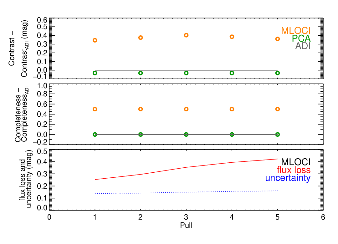
In Figures 6–10, we compare average detection statistics from our 10 NICI datasets for basic ADI, PCA and MLOCI for different reduction parameters. In Figure 6, we see that the performance of MLOCI is not very sentitive to , the relative intensity of the negative sources, generally yielding contrast improvements of 0.3-0.4 mag. The plots are made for =2.15 and optimum parameter settings =16 and =2. However, for very large (e.g. 10–100) we have found that the performance of MLOCI does deteriorate. Moreover, the counterpart PSFs begin to look similar to each other, instead of the science images that they are being matched to. This is because LOCI strongly biases the linear combination to match the negative sources in the counterpart images. The completeness improvement for MLOCI at the chosen threshold is usually 50%. The ADI and PCA performances are nearly equal to each other.
From our reduction experiments, we can estimate the accuracy of the photometric measurements allowed by MLOCI. The systematic uncertainty of the photometry can be estimated by the change in the contrast before and after recovery, between the companion in the test sector to the two point sources in the reference sector. Since the reduction is done 10 times with the reference companions in different positions, we can also estimate the random uncertainty by calculating the standard deviation of the contrast after recovery between the two sets of companions. When an actual companion is detected in a real dataset, we can estimate photometric uncertainties and systematic errors by injecting companions at other PAs at the same separation and performing MLOCI reductions to recover them. In the bottom panel of Figure 6, we see that while the photometric uncertainty is insentitive to (variation of 13% in these cases), the systematic error increases with increasing .
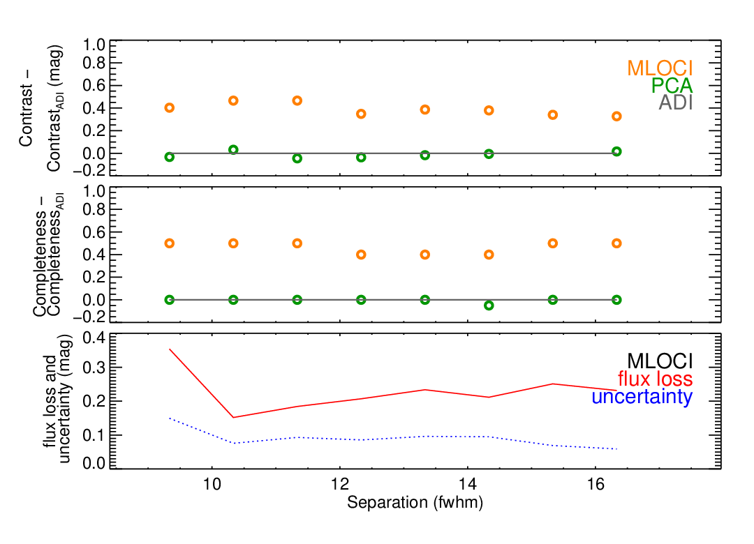
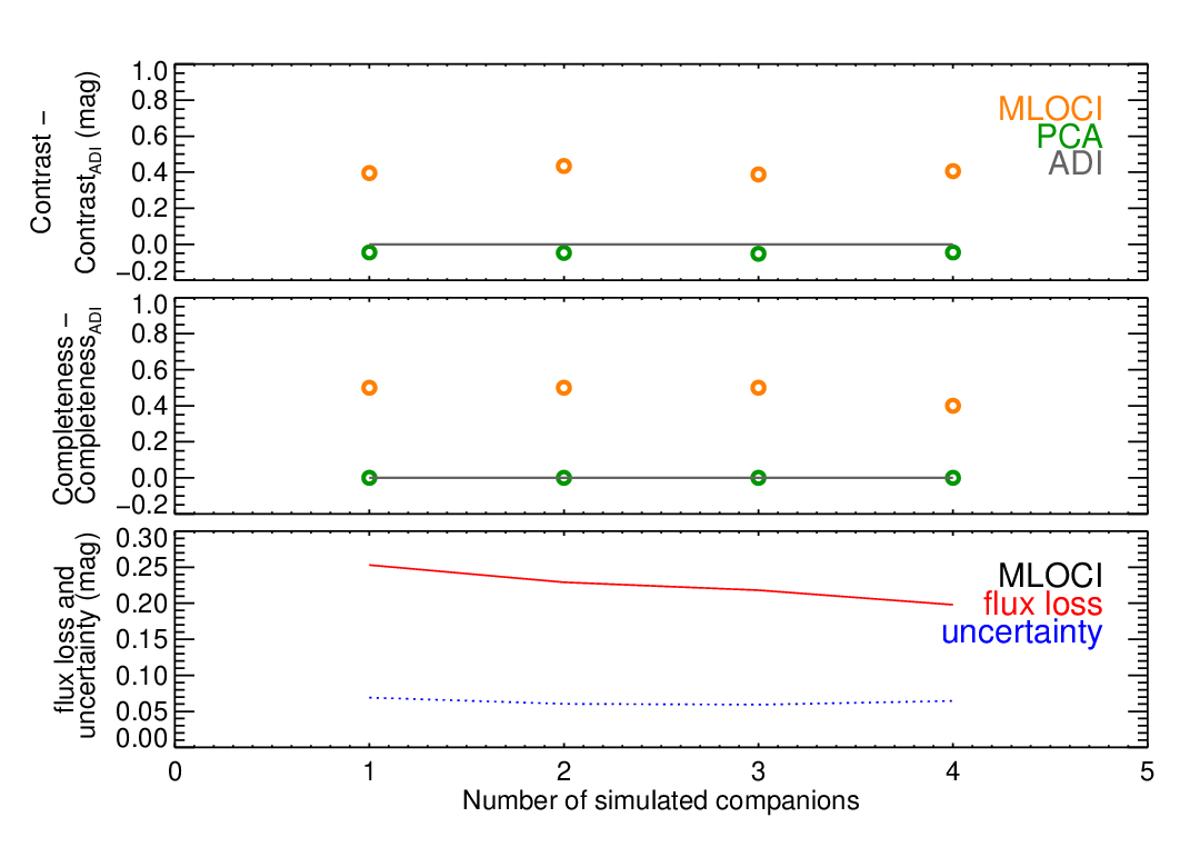
In Figures 6–8, we see that the contrast (and completeness) improvements are not very sensitive to the width of the reference sector or the number of companions used as reference, or the separation of the recovered companions from the primary. However, Figure 10 shows that for very small sky rotation (0.35) the contrast gain due to MLOCI is much larger (1.4 mag). Here, PCA also shows a 0.5 mag gain over ADI. The variation of photometric uncertainties over these experiments is small.
In Figure 11, we show attempts at measuring the source properties at the test locations after 800 MLOCI reductions of the UY Pic data set when no actual signal has been injected. According to the previously defined detection criteria in §4, none of the measurements satisfied the detection crtieria and thus no false positives were detected. Moreover, the standard deviation of the SNR distribution was 1.0, showing that the false positive rate is not elevated above that expected. A higher false positive rate would indicate that while the reduction method may produce detections with seemingly high SNR, the noise is in fact not being calculated correctly.
We also performed non-blind reduction experiments where the test companion and the reference companions are treated the same by MLOCI, using negative sources in all locations when creating the counterpart PSFs and/or positive sources when combining all the images. In these cases, the apparent contrast improvement was on average 0.75 mag. However, using the best algorithm parameters we were only able to reduce the false detection rate to 1%. Poor parameters could yield false detection rates 20%. Thus, MLOCI must be kept blind about any suspected companion, except when informed by another blind process, which in our case is a basic ADI reduction. By the same logic, other versions of LOCI and PCA can also accidentally create false detections, since no restrictions on the allowed linear combinations are generally imposed when constructing reference images. This is an especially unpleasant possibility when trying to re-detect a companion marginally detected in an earlier epoch. We therefore strongly recommend that FDRs be provided for any reduction method.
IV.3 GPI Early Science Data
Here, we describe the results of MLOCI and ADI processing of the GPI data on HD 135344 B. In Figure 3a, we show a de-rotated median combination of all the channels without PSF subtraction, but scaled in intensity by 2, and then bandpass filtered to isolate spatial features between 2–8 pixels. We easily see the spiral arms, discovered in Muto et al. [17], extending out to 0.9′′, and the cavity inside 0.2′′. However, we do not see their inner ring where the spiral arms begin. We do see a bright rim at 0.15′′ separation around the coronagraphic mask. Since, there is presumably no self-subtraction of the disk (no ADI) in this image, we use this image to identify reliable signal and background regions for MLOCI (Figure 3d).
In the regular ADI reduction (Figure 3b) we find some features at 110–170 mas separations with SNR=3–5 (=8-9.5 mag), particularly two radially extended spots to the NE and SW. As discussed in Menard et al. (2015, in preparation), while these could prove to be accretion streams from the disk onto the star, this is currently uncertain because of the small amount of sky motion (1.7–2FWHM) at the relevant separation and similar PSF features in the unreduced images near mask (see Figure 3a). Moreover, GPI images of HR 4796 A [19] also show similar residuals near the mask.
We find that particular caution needs to be exercised with MLOCI when there is signal in the FoV which is extended azimuthally, as in the case of HD 135344 B. When we try to target each spot separately with non-blind MLOCI, we obtain isolated point sources, admittedly with large FWHM, while the rest of the disk disappears (see Figures 3c). This demonstrates the ability of non-blind algorithms which allow free linear combinations of science images to produce misleading features, especially in the case where disk emission may exist. In the absence of disk emission, we have found that the most conservative non-blind methods create less false positives but still at elevated levels compared to ADI.
However, the MLOCI algorithm for extended-sources does have the special ability to improve the SNR of any feature suspected in a dataset, be it mutiple companions or an entire disk. To demonstrate this potential of the algorithm, we use MLOCI (=3; extended-source reduction as described in §2 & §3) to optimize the SNR according to regions selected in Figure 3d. Indeed, the spiral and the suspected streamers are much enhanced in the MLOCI reduction (see Figure 3e). When we flip the matching regions vertically so that they do not match with the real disk emission, MLOCI yields no disk (Figure 3f). Thus MLOCI is not likely to yield false disk detections.
V CONCLUSIONS
We have presented a version of the LOCI algorithm that significantly improves the SNR of both point and extended sources. This algorithm, called Matched LOCI or MLOCI, can be applied to both ADI and IFS data. The only difference being that, in the PSF construction step of image processing, the images have to be pupil aligned in the former and both pupil and spectrally aligned in the latter. The contrast gain over both regular ADI and PCA in NICI data was 0.3-1.4 mag. This is especially interesting, since it was shown that LOCI itself provides no gain over regular ADI processing for NICI data [25]. While we found that LOCI could reduce the speckle noise in the final reduced image, it also reduced the signal of test companions.
We have shown how MLOCI can be used in the detection of disks using GPI data, recovering new streamer-like features which need new observations before they can be confirmed. Thus MLOCI can be a powerful tool for the detection of companions and disks in the current direct imaging campaigns with GPI and SPHERE.
While, for blind MLOCI the false detection rate is low, we found that for non-blind MLOCI for both NICI and GPI data, the false detection rate (FDR) can in some cases be much higher. The FDR is even more for when there is azimuthally distributed diffuse light in the FoV. Thus, in non-blind variants of LOCI and PCA algorithms high FDRs may also arise. Therefore, we strongly recommend that FDRs be measured whenever these methods are used.
Facilities: Gemini-South (GPI, NICI).
References
- [1] Amara, A., & Quanz, S. P. 2012, MNRAS, 427, 948
- [2] Beuzit, J.-L., et al. 2010, in Astronomical Society of the Pacific Conference Series, Vol. 430, Pathways Towards Habitable Planets, ed. V. Coudé Du Foresto, D. M. Gelino, & I. Ribas, 231
- [3] Biller, B. A., Liu, M. C., Wahhaj, Z., Nielsen, E. L., Hayward, T. L., et al. 2013, ApJ, 777, 160
- [4] Biller, B. A., et al. 2007, ApJS, 173, 143
- [5] Currie, T., et al. 2013, ApJ, 776, 15
- [6] Garufi, A., et al. 2013, A&A, 560, A105
- [7] Lafrenière, D., Marois, C., Doyon, R., Nadeau, D., & Artigau, É. 2007, ApJ, 660, 770
- [8] Liu, M. C. 2004, Science, 305, 1442
- [9] Liu, M. C., et al. 2010, in Society of Photo-Optical Instrumentation Engineers (SPIE) Conference Series, Vol. 7736, Society of Photo-Optical Instrumentation Engineers (SPIE) Conference Series
- [10] López-Santiago, J., Montes, D., Crespo-Chacón, I., & Fernández-Figueroa, M. J. 2006, ApJ, 643, 1160
- [11] Macintosh, B. A., et al. 2008, in Society of Photo-Optical Instrumentation Engineers (SPIE) Conference Series, Vol. 7015, Society of Photo-Optical Instrumentation Engineers (SPIE) Conference Series
- [12] Maire, J., et al. 2010, in Society of Photo-Optical Instrumentation Engineers (SPIE) Conference Series, Vol. 7735, Society of Photo-Optical Instrumentation Engineers (SPIE) Conference Series
- [13] Marois, C., Correia, C., Galicher, R., Ingraham, P., Macintosh, B., Currie, T., & De Rosa, R. 2014, ArXiv e-prints
- [14] Marois, C., Doyon, R., Racine, R., Nadeau, D., Lafreniere, D., Vallee, P., Riopel, M., & Macintosh, B. 2005, JRASC, 99, 130
- [15] Mawet, D., et al. 2014, ArXiv e-prints
- [16] McBride, J., Graham, J. R., Macintosh, B., Beckwith, S. V. W., Marois, C., Poyneer, L. A., & Wiktorowicz, S. J. 2011, PASP, 123, 692
- [17] Muto, T., et al. 2012, ApJ, 748, L22
- [18] Nielsen, E. L., et al. 2013, ApJ, 776, 4
- [19] Perrin, M. D., et al. 2014, ArXiv e-prints
- [20] Pueyo, L., et al. 2012, ApJS, 199, 6
- [21] Racine, R., Walker, G. A. H., Nadeau, D., Doyon, R., & Marois, C. 1999, PASP, 111, 587
- [22] Soummer, R., Pueyo, L., & Larkin, J. 2012, ApJ, 755, L28
- [23] Sparks, W. B., & Ford, H. C. 2002, ApJ, 578, 543
- [24] Thatte, N., Abuter, R., Tecza, M., Nielsen, E. L., Clarke, F. J., & Close, L. M. 2007, MNRAS, 378, 1229
- [25] Wahhaj, Z., Liu, M. C., Biller, B. A., Nielsen, E. L., Hayward, T. L., et al. 2013a, ApJ, 779, 80
- [26] Wahhaj, Z., Liu, M. C., Nielsen, E. L., Biller, B. A., Hayward, T. L., et al. 2013b, ApJ, 773, 179
- [27] Wahhaj, Z., et al. 2011, ApJ, 729, 139