跳到论文正文
W Papers独立论文阅读器 arXiv:1502.02940 论文正文 计算阅读时间 · 0%
引用这篇论文根据当前论文元数据生成,正式投稿前建议核对。


License: arXiv.org perpetual non-exclusive license
arXiv:1502.02940v1 [cs.IT] 10 Feb 2015
\authoruppercase

MUHAMMET FATİH BAYRAMOG̃LU \graduateschoolNatural and Applied Sciences \shortdegreePh.D. \directorProf. Dr. Canan Özgen \headofdeptProf. Dr. İsmet Erkmen \degreeDoctor of Philosophy \departmentElectrical and Electronics Engineering \supervisorAssoc. Prof. Dr. Ali Özgür Yılmaz \departmentofsupervisorElectrical and Electronics Engineering Dept., METU \turkishtitleOlasilik KÜtlesİ FonksİyonlarInIn Hİlbert UzayI
ve OlasIlIsIksal Bİlgİ ÇIkarImI Üzerİne UygulamalarI \turkishdegreeDoktora \turkishdepartmentElektrik Elektronik Mühendislig̃i Bölümü \turkishdateEylül 2011 \turkishsupervisorDoç. Dr. Ali Özgür Yılmaz \anahtarklmOlasılık kütlesi fonksiyonlarının Hilbert uzayı, Olasılık kütlesi fonksiyonlarının çarpanlara ayrılması, olasılısıksal bilgi çıkarımı, çok-girdili çok-çıktılı sezim, Markov rastgele alanlar \committeememberiProf. Dr. Yalçın Tanık \committeememberiiAssoc. Prof. Dr. Ali Özgür Yılmaz \committeememberiiiProf. Dr. Mustafa Kuzuog̃lu \committeememberivAssoc. Prof. Dr. Emre Aktaş \committeemembervAssist. Prof. Dr. Ayşe Melda Yüksel \affiliationiElectrical and Electronics Eng. Dept., METU \affiliationiiElectrical and Electronics Eng. Dept., METU \affiliationiiiElectrical and Electronics Eng. Dept., METU \affiliationivElectrical and Electronics Eng. Dept., Hacettepe University \affiliationvElectrical and Electronics Eng. Dept.,
TOBB University of Economy and Technology

{preliminaries}

The Hilbert Space of Probability Mass Functions
and Applications on Probabilistic Inference

Muhammet Fatih Bayramog̃lu
September 2011
Abstract
\oneandhalfspacing

The Hilbert space of probability mass functions (pmf) is introduced in this thesis. A factorization method for multivariate pmfs is proposed by using the tools provided by the Hilbert space of pmfs. The resulting factorization is special for two reasons. First, it reveals the algebraic relations between the involved random variables. Second, it determines the conditional independence relations between the random variables. Due to the first property of the resulting factorization, it can be shown that channel decoders can be employed in the solution of probabilistic inference problems other than decoding. This approach might lead to new probabilistic inference algorithms and new hardware options for the implementation of these algorithms. An example of new inference algorithms inspired by the idea of using channel decoder for other inference tasks is a multiple-input multiple-output (MIMO) detection algorithm which has a complexity of the square-root of the optimum MIMO detection algorithm.

keywords
The Hilbert space of pmfs, factorization of pmfs, probabilistic inference, MIMO detection, Markov random fields
\makeapproval\plagiarism
{oz}\oneandhalfspacing

Bu tezde olasılık kütlesi fonksiyonlarının Hilbert uzayı sunulmaktadır. Bu Hilbert uzayının sag̃ladıg̃ı olanaklar kullanılarak çok deg̃işkenli olasılık kütlesi fonksiyonlarını çarpanlarına ayırmak için bir yöntem önerilmiştir. Bu yöntemden elde edilen çarpanlara ayırma iki nedenle özeldir. İlk olarak, bu çarpanlara ayırma rastgele deg̃işkenler arasındaki cebirsel bag̃ıntıları ortaya koyar. İkinci olarak, rastgele deg̃işkenler arasındaki koşullu bag̃ımsızlık ilişkilerini belirler. Birinci özellik sayesinde kanal kod çözücülerinin, kod çözmekten başka olasılıksal bilgi çıkarımı problemlerinin çözümünde de kullanılabileceg̃i gösterilebilir. Bu yaklaşım yeni olasılıksal bilgi çıkarımı algoritmalarına ve bu algoritmaları gerçeklemek için yeni donanım olanaklarına yol açabilir. Kod çözücülerin kod çözmekten başka bilgi çıkarımı görevlerinde kullanılması fikrinden esinlenen algorıtmaların bir örneg̃i, karmaşıklıg̃ı en iyi algoritmanın karekökü olan bir çok-girdili çok-çıktılı sezim algoritmasıdır.

\dedication

Karıma
To my wife

Acknowledgements.
\oneandhalfspacingFirstly, I would like to thank sincerely my supervisor Assoc. Prof. Dr. Ali Özgür Yılmaz. He is an exception in this department regarding both his scientific vision and his personality. His trust and encouragement was crucial to me while working on this thesis. I would like to thank the members of the thesis progress monitoring committee members Prof. Dr. Mustafa Kuzuog̃lu and Assoc. Prof. Dr. Emre Aktaş for their valuable comments and contributions. Moreover, operator theory course of Prof. Kuzuog̃lu helped me a lot in this thesis. Furthermore, I appreciate the financial support that Assoc. Prof. Aktaş provided to me in the last periods of my thesis study and his understanding. I would like to thank also the rest of thesis jury members Prof. Dr. Yalçın Tanık and Assist. Prof. Dr. Melda Yüksel for their valuable comments. I would like express my gratitude to the other two exceptional faculty members of this department who are Prof. Dr. Arif Ertaş and Assoc. Prof. Dr. Çag̃atay Candan. Prof. Ertaş is a person really deserving his name “Arif”. Assoc. Prof. Candan is one of the easiest persons that I can communicate with and I appreciate his “always open” door. I would like to thank Prof. Dr. Zafer Ünver. I learned a lot from him while assisting EE213 and EE214 courses. Education is a long haul run. Hence, sincere thanks go to my high school mathematics teachers Ahmet Cengiz, Hüseyin Çakır, Perihan Özdingiş, and of course Demir Demirhas. A special thanks goes to my undergraduate advisor Prof. Dr. Gönül Turhan Sayan. I would like to acknowledge the free software community. I have never needed and used any commercial software during my Ph.D. research. I would like to thank Dr. Jorge Cham for phdcomics which introduced some smiles to our overly stressed lives. I would like to thank my friends Alper Söyler, Murat Kılıç, Mehmet Akif Antepli, Murat Üney, Yılmaz Kalkan, Serdar Gedik, and Onur Özeç for their valuable friendship. My sincere gratitude goes to my parents Nezahat and Mustafa Bayramog̃lu. This thesis could not finish without their prayers. But the good manners I learned from them is much more valuable to me than this Ph.D. degree. I would like to thank my brother Etka for being the kindest brother in the world. My deepest thanks goes to my wife Neslihan, or more precisely Dr. Neslihan Yalçın Bay-ramog̃lu. I appreciate everything she sacrificed for me. I studied on this thesis on times that I stoled from her and she really deserves at least the half of the credit for this thesis. Her support not only was vital for me during the Ph.D. but also will continue to be vital during the rest of my life.

This thesis summarizes the research work carried out in six years starting from September 2005. The research topic arose while I was trying to develop an analysis method for the convergence rate of the iterative sum-product algorithm. Since the messages (beliefs) passed between the nodes in the iterative sum-product algorithm are probability mass functions (pmf), I thought that representing the pmfs in a Hilbert space structure would prove useful in the analysis of the sum-product algorithm. Analyzing the convergence of the sum-product algorithm would be an application of the norm in the Hilbert space of pmfs. However, later I noticed that the inner product has much more interesting applications and preferred focusing on the applications of the inner product to dealing with the convergence which led to this thesis.

In order to read the thesis a basic understanding of inner product spaces and finite fields is necessary. Anybody with this background can follow the chapters from the second to the fifth. I believe that these chapters are the core of the thesis. Chapter 6 contains some applications from communication theory and might require a communication theory background.

This preface is an adequate place to note some observations about my country and university. I am happy to observe that Turkey improved economically and democratically during my graduate studies. On the other hand, I am sad to observe that Middle East Technical University downgraded scientifically and democratically during the same time.

This thesis is related probability theory. Probability theory is an area which is close to the border between science and belief. Although Laplace’s book on celestial mechanics misses to mention God, my explanation on the relation between probability and willpower makes me to believe in God and I would like to start to the rest of the thesis by a quote from the translation of Qur’an which explains what is science to me: “Glory be to You, we have no knowledge except what you have taught us. Verily, it is You (Allah), the All-Knower, the All-Wise”.

Chapter 1 INTRODUCTION

1 Motivation

A linear vector space structure over a set provides algebraic tools such as addition and scaling to carry out on the elements of the set. If a vector space can be endowed with an inner product then it becomes an inner product space. An inner product provides geometric concepts such as norm, distance, angle, and projections. If every Cauchy sequence in an inner product space converges with respect to the inner product induced norm then the inner product space becomes a Hilbert space. Needless to say a Hilbert space structure is very useful and find application areas in diverse fields of science. Communication theory is not an exception. For instance, the signal space representation in communication theory relies on the Hilbert space structure constructed over the set of square integrable functions.

One of the mathematical objects that is too frequently used in communication and information theories is the probability mass functions (pmf) which are discrete equivalents of probability density functions. Although, pmfs are so frequently used in communication and information theories a Hilbert space structure for them was missing. A Hilbert space of pmfs might have many interesting applications.

A possible application for the Hilbert space of probability mass functions might be analyzing the characteristics of a multivariate pmf. An important characteristic of a multivariate pmf is the conditional independence relations imposed by it. The conditional independence relation imposed by a multivariate pmf is determined by the factorization of the pmf to local functions11 1 Local functions are functions (not necessarily pmfs) which have less arguments than the original multivariate pmf. as explained in [18, 19].

The factorization structure of a multivariate pmf into local functions also determines the algorithms which can perform inference on the pmf, in other words, maximize or marginalize the pmf. The sum-product algorithm, which is also called belief propagation, and the max-product algorithm effectively marginalize or maximize a multivariate pmf by exploiting the pmfs’ factorization structure [1]. Modern decoding algorithms such as low-density parity-check decoding and turbo decoding, which have become highly popular in the last decade, relies on this fact.

Some multivariate pmfs, for instance the pmf resulting from a hidden Markov model, has an apparent factorization structure. However, one cannot be sure whether this factorization structure is the “best” possible factorization or not. On the other hand, some pmfs, for instance the pmfs obtained empirically, might not have an apparent factorization structure at all. Therefore, developing a method which obtains the factorization of a multivariate pmf systematically would prove useful in many areas.

2 Contributions

The first contribution in this thesis is the derivation of the Hilbert space structure for pmfs. The Hilbert space of pmfs not only provides a vectorial representation of evidence but also it proves to be a useful tool in analyzing the pmfs.

The second contribution of this thesis is a systematic method for obtaining factorization of a multivariate pmf. The resulting factorization is unique and is the ultimate factorization possible. Hence, we call the resulting factorization as the canonical factorization. The canonical factorization of a multivariate pmf is obtained by projecting the pmf onto orthogonal basis pmfs of the Hilbert space of pmfs. Hence, this factorization method heavily relies on the Hilbert space of pmfs.

The basis pmfs mentioned in the paragraph above are special pmfs such that their value is determined only by a linear combination of their arguments. In order to be able to talk about linear combinations of arguments addition and multiplication must be well defined between arguments of the pmf. Hence, the canonical factorization of a pmf can be obtained only if the pmf is a pmf of finite-field-valued random variables. This is an important limitation of the canonical factorization.

The property of the basis pmfs mentioned in the previous paragraph causes an important limitation but also this property leads to the third and the probably the most important contribution of the thesis. Since the basis pmfs are functions of their arguments, the canonical factorization reveals the algebraic dependencies between the random variables. Thanks to this fact, it can be shown that channel decoders can be employed as an apparatus for tasks beyond decoding. This idea leads to new hardware options as well as new inference algorithms.

The fourth contribution of the thesis is an application of the idea explained in the paragraph above. This contribution is a multiple-input multiple-ouput (MIMO) detection algorithm which employs the decoder of a tail biting convolutional code as a processing device. This algorithm is an approximate soft-input soft-output MIMO detection algorithm whose complexity is the square-root of that of the optimum MIMO detection algorithm.

The final contribution of the thesis is another property of the canonical factorization. It can be shown that the conditional dependence relationships imposed by a multivariate pmf can be determined from the canonical factorization of the pmf. In other words, the conditional independence relationships imposed by a pmf can be determined by using the geometric tools provided by the Hilbert space of pmfs. This property of the canonical factorization might lead to applications in experimental fields such as bioinformatics dealing with large amounts of data.

3 Comparison to earlier work

A Hilbert space of probability density functions is first presented in literature in a very different area of science, stochastic geology, in [4]. Their derivation is for a class of continuous probability density functions. On the other hand our derivation is for pmfs. Although, the resulting Hilbert space structures in both their and our derivations are quite similar, our derivation is independent of theirs. Furthermore, we provide many applications of the Hilbert space of pmfs on probabilistic inference.

The canonical factorization proposed in this thesis can be compared to the factorization of pmfs provided by the Hammersley-Clifford theorem [18, 19]. Both the Hammersley-Clifford theorem and the canonical factorization can completely determine the conditional independence relationships imposed by a pmf. But Hammersley-Clifford theorem does not highlight the algebraic dependence relationships between random variables while the canonical factorization does. Moreover, the canonical factorization is unique whereas the factorization of the Hammersley-Clifford theorem is not.

The results obtained in this thesis can be located in the factor graph literature as follows. Factor graphs are bipartite graphical models which represent the factorization of a pmf [1]. The bipartite graphs were first employed by Tanner to describe low complexity codes in [5]. A very crucial step in achieving the factor graph representation is the Ph.D. thesis of Wiberg [6, 7]. In his thesis Wiberg showed the connection between various codes and decoding algorithms by introducing hidden state nodes to the graphs described by Tanner and characterized the message passing algorithms running on these graphs. Local constraints in [6] are behavioral constraints, such as parity check constraints. The factor graphs are the generalization of the graphical models introduced in [6] by allowing local constraints to be arbitrary functions rather than behavioral constraints [1].

The canonical factorization proposed in this thesis can also be represented by a factor graph. Moreover, the factor functions appearing in the canonical factorization can be transformed into usual parity check constraints by introducing some auxiliary variables. Therefore, the factor graph representing the canonical factorization can be transformed into a Tanner graph by introducing some auxiliary variable nodes which are very different from the hidden state nodes introduced in [6]. This is essentially an explanation of the claim that the channel decoders can be employed for inference tasks beyond decoding.

4 Outline

After this chapter, the thesis continues with the introduction of the Hilbert space of pmfs in Chapter 2. The Hilbert space of pmfs is the main tool to be used throughout the thesis. The canonical factorization is introduced in Chapter 3. Chapter 4 investigates the properties and special cases of the canonical factorization. Chapter 5 explains how a channel decoder can be used for other probabilistic inference tasks other than its own purpose. This explanation is based on the canonical factorization. Some possible consequences of this result are also explained in Chapter 5. Chapter 6 provides some basic examples from communication theory on the use of channel decoders for other inference tasks beyond decoding. The MIMO detector which uses the decoder of a tail biting convolutional code is also introduced in this chapter. Chapter 7 shows that the conditional independence relations can be completely determined from the canonical factorization. The thesis is concluded with some possible future directions in Chapter 8. For the sake of neatness of the thesis some proofs and derivations are collected in the Appendix.

5 Some remarks on notation

Throughout the thesis we denote the deterministic variables with lowercase letters and random variables with uppercase letters. We represent functions of multiple variables as functions of vectors and denote vectors with boldface letters. Lowercase boldface letters denote deterministic vectors and capital boldface letters denote random variables. All vectors encountered in the thesis are row vectors except a few cases in Chapter 6.

Matrices are also denoted with capital boldface letters which might lead to a confusion with random vectors. Throughout the thesis, we used 𝐕\mathbf{V}, 𝐖\mathbf{W}, 𝐗\mathbf{X}, 𝐘\mathbf{Y}, and 𝐙\mathbf{Z} to denote random vectors. All the other capital boldface letters are matrices.

Unfortunately, many different types of additions are included in the thesis such as finite field addition, real number addition, vector addition, and even direct sum of subspaces. We reserve ⊕\oplus symbol for the direct sum of subspaces for the sake of consistency with the linear algebra literature. We use ⊞\boxplus symbol for the vectorial addition operation of pmfs which is defined in Chapter 2. We have to use the remaining ++ symbol for all the rest of addition operations such as real number addition, finite field addition, and vectorial addition in ℝN\mathbb{R}^{N}. Fortunately, the type of the addition employed can be determined from the types of the operands.

A possible confusion might arise while using the summation symbol ∑\sum. For instance, ∑i=1Npi​(x)\sum_{i=1}^{N}p_{i}(x) might refer to both p1​(x)+p2​(x)+…+pN​(x)p_{1}(x)+p_{2}(x)+\ldots+p_{N}(x) and p1​(x)⊞p2​(x)⊞…⊞pN​(x)p_{1}(x)\boxplus p_{2}(x)\boxplus\ldots\boxplus p_{N}(x) which are really two different summations. In order to avoid this confusion we denote the latter summation with ∑i=1N⊞​pi​(x)\sideset{{}^{\boxplus}}{}{\sum}_{i=1}^{N}p_{i}(x), although summations like the former is never encountered in the thesis.

Chapter 2 THE HILBERT SPACE OF PROBABILITY MASS FUNCTIONS

6 Introduction

The Hilbert space of probability mass functions (pmf), which is the main tool to be employed in the thesis, is introduced in this chapter. Throughout the thesis we are only interested in the pmfs of the finite-field-valued random variables. Therefore, we define what a finite-field-valued random variable is first in Section 7. We introduce the set of pmfs on which we construct the Hilbert space in Section 8. Then we construct the algebraic and geometric structures over this set in Section 9 and Section 10 respectively. Section 11 emphasizes the differences between the Hilbert space of random variables and the Hilbert space of pmfs in order to avoid possible confusion. Finally, in Section 12 the idea of the construction of the Hilbert space is repeated on the set of multivariate pmfs.

7 Finite-Field-Valued Random Variables

Traditionally a random variable is a mapping from the event space to the real or complex fields. However, in some experiments, e.g., the experiments with discrete event spaces, it might be useful to map the outcomes of the experiment to a finite (Galois) field. Such a mapping would allow to carry out meaningful algebraic operations between the outcomes of different experiments, for instance as in [32]. A finite-field-valued random variable is defined below.

Definition 1

Finite-field-valued random variable: Let Ω\Omega be the event space of an experiment and 𝔽q=GF⁡(q)\mathbb{F}_{q}=\mathrm{GF}(q) be the finite field of qq elements. Moreover, let a function X:Ω→𝔽qX:\Omega\rightarrow\mathbb{F}_{q} be defined as

X⁡(ω∈ℰi)≜i∀i∈𝔽q​,X(\omega\in\mathcal{E}_{i})\triangleq i\quad\forall i\in\mathbb{F}_{q}\textrm{,}

where {ℰi:i∈𝔽q}\{\mathcal{E}_{i}:i\in\mathbb{F}_{q}\} are events (subsets of Ω\Omega) of this experiment. The function XX is called an 𝔽q\mathbb{F}_{q}-valued random variable if the events {ℰi:i∈𝔽q}\{\mathcal{E}_{i}:i\in\mathbb{F}_{q}\} are mutually exclusive and collectively exhaustive, i.e.,

ℰi≠ℰj\displaystyle\mathcal{E}_{i}\neq\mathcal{E}_{j} ⟹\displaystyle\implies ℰi∩ℰj=∅∀i,j∈𝔽q​,\displaystyle\mathcal{E}_{i}\cap\mathcal{E}_{j}=\emptyset\quad\forall i,j\in\mathbb{F}_{q}\textrm{,}
⋃i∈𝔽qℰi\displaystyle\bigcup_{i\in\mathbb{F}_{q}}\mathcal{E}_{i} =\displaystyle= Ω​.\displaystyle\Omega\textrm{.}

Actually, we do not need to restrict ourselves to the finite-field-valued random variables in this chapter since the ideas presented in this chapter can be applied to any discrete random variable. We need the concept of finite-field-valued random variables starting from the next chapter. However, we introduce the finite-field-valued random variables starting from this chapter in order to make the representation simpler.

8 The Set of Strictly Positive Probability Mass Functions

Many different experiments can be represented with an 𝔽q\mathbb{F}_{q}-valued random variable. All these experiments may lead to different pmfs. Furthermore, we may have different pmfs even for the same experiment if the outcome is conditioned on some other event. Let 𝒫𝔽q\mathcal{P}_{\mathbb{F}_{q}} be the set of all strictly positive pmfs that an 𝔽q\mathbb{F}_{q}-valued random variable might possess, i.e.,

𝒫𝔽q≜{p⁡(x):𝔽q→(0,1)⊂ℝ​ s.t. ​∑x∈𝔽qp⁡(x)=1}​.\mathcal{P}_{\mathbb{F}_{q}}\triangleq\left\{p(x):\mathbb{F}_{q}\rightarrow(0,1)\subset\mathbb{R}\textrm{ s.t. }\sum_{x\in\mathbb{F}_{q}}p(x)=1\right\}\textrm{.} (1)

The Hilbert space of pmfs is going to be constructed on 𝒫𝔽q\mathcal{P}_{\mathbb{F}_{q}}. This set excludes the pmfs which take value zero for some values. The reason under this restriction will be clear after scalar multiplication is defined on this set.

We are going to represent the pmfs with lowercase letters such as p⁡(x)p(x), r⁡(x)r(x), or s⁡(x)s(x). These pmfs may represent the pmfs of random variables representing different experiments as well as they may represent the pmfs of the same random variable conditioned on different events.

8.1 The normalization operator

We employ a normalization operator to obtain pmfs from strictly positive real-valued functions by scaling them. We denote this normalization operator with 𝒞𝔽q{.}\mathcal{C}_{\mathbb{F}_{q}}\left\{.\right\} and define it as

𝒞𝔽q​{α⁡(x)}:ℱ𝔽q→𝒫𝔽q≜α⁡(x)∑i∈𝔽qα⁡(i)​,\mathcal{C}_{\mathbb{F}_{q}}\left\{\alpha(x)\right\}:\mathcal{F}_{\mathbb{F}_{q}}\rightarrow\mathcal{P}_{\mathbb{F}_{q}}\triangleq\frac{\alpha(x)}{\sum_{i\in\mathbb{F}_{q}}\alpha(i)}\textrm{,} (2)

where the set ℱ𝔽q\mathcal{F}_{\mathbb{F}_{q}} denotes the set of all functions from 𝔽q\mathbb{F}_{q} to ℝ+\mathbb{R}^{+} and α⁡(x)\alpha(x) is a function in ℱ𝔽q\mathcal{F}_{\mathbb{F}_{q}}. An obvious property of the operator 𝒞𝔽q{.}\mathcal{C}_{\mathbb{F}_{q}}\left\{.\right\} that we exploit frequently is given below

𝒞𝔽q​{β​α​(x)}=𝒞𝔽q​{α⁡(x)}​,\mathcal{C}_{\mathbb{F}_{q}}\left\{\beta\alpha(x)\right\}=\mathcal{C}_{\mathbb{F}_{q}}\left\{\alpha(x)\right\}\textrm{,} (3)

where β\beta is any positive number.

9 The Algebraic Structure over 𝒫𝔽q\mathcal{P}_{\mathbb{F}_{q}}

The foundation of the Hilbert space of PMFs is the addition operation. Hence, the definition of the addition should be meaningful in the sense of probabilistic inference in order to take advantage of the Hilbert space structure for inference problems.

The addition operation is inspired by the following scenario. Assume that we receive information about a uniformly distributed source XX via two independent channels with outputs y1y_{1} and y2y_{2} as depicted in Figure 1. Let p⁡(x)=Pr⁡{X=x|y1}p(x)=\Pr\{X=x|y_{1}\}, q⁡(x)=Pr⁡{X=x|y2}q(x)=\Pr\{X=x|y_{2}\}, and r(x)=Pr{X=x|y1,y2}r(x)=\Pr\{X=x|y_{1},y_{2}\}. Since XX is uniformly distributed, r⁡(x)r(x) can be derived as

r⁡(x)\displaystyle r(x) =\displaystyle= p⁡(x)​q​(x)∑x∈𝔽qp⁡(x)​q​(x)\displaystyle\frac{p(x)q(x)}{\sum_{x\in\mathbb{F}_{q}}p(x)q(x)} (4)
=\displaystyle= 𝒞𝔽q​{p⁡(x)​q​(x)}\displaystyle\mathcal{C}_{\mathbb{F}_{q}}\left\{p(x)q(x)\right\} (5)

by employing the Bayes’ theorem.

The PMFs p⁡(x)p(x) and q⁡(x)q(x) represent the evidence about the source XX when only y1y_{1} or y2y_{2} is known respectively. On the other hand, r⁡(x)r(x) represents the total evidence when both outputs are known. In a way, r⁡(x)r(x) is obtained by summing p⁡(x)p(x) and q⁡(x)q(x). Hence, (4) can be adopted as the definition of addition. For any p⁡(x)p(x) and q⁡(x)q(x) in 𝒫𝔽q\mathcal{P}_{\mathbb{F}_{q}} their addition is denoted by ⊞\boxplus and defined as

p⁡(x)⊞q⁡(x)≜𝒞𝔽q​{p⁡(x)​q​(x)}​.p(x)\boxplus q(x)\triangleq\mathcal{C}_{\mathbb{F}_{q}}\left\{p(x)q(x)\right\}\textrm{.} (6)

The definition of the addition operation is such a critical point of this thesis that the rest of the thesis will be built upon this definition.

This definition of addition operation is the same as parallel information combining operation as defined in [13] and message computation at variable nodes in the sum-product algorithm [1].

Refer to caption
Figure 1: The scenario for explaining the meaning of addition operation.

Defining the addition operation also enforces the scalar multiplication to have such a form that scalar multiplication is consistent with the addition. The scalar multiplication, which is denoted by ⊠\boxtimes, should satisfy the relation below for positive integers nn

n⊠p⁡(x)\displaystyle n\boxtimes p(x) =\displaystyle= p⁡(x)⊞p⁡(x)⊞…⊞p⁡(x)⏟n times\displaystyle\underbrace{p(x)\boxplus p(x)\boxplus\ldots\boxplus p(x)}_{\textrm{n times}} (7)
=\displaystyle= 𝒞𝔽q​{(p⁡(x))n}​.\displaystyle\mathcal{C}_{\mathbb{F}_{q}}\left\{(p(x))^{n}\right\}\textrm{.}

Generalizing (7) to any α\alpha in ℝ\mathbb{R} leads to the definition of scalar multiplication below

α⊠p⁡(x)≜𝒞𝔽q​{(p⁡(x))α}​.\alpha\boxtimes p(x)\triangleq\mathcal{C}_{\mathbb{F}_{q}}\left\{(p(x))^{\alpha}\right\}\textrm{.} (8)

In order to be able to scale p⁡(x)p(x) with negative coefficients it is necessary that p⁡(x)≠0p(x)\neq 0 for any xx in 𝔽q\mathbb{F}_{q}. Hence, in the definition of 𝒫𝔽q\mathcal{P}_{\mathbb{F}_{q}} an open interval is used rather than a closed interval in (1).

Theorem 2.1

The set 𝒫𝔽q\mathcal{P}_{\mathbb{F}_{q}} together with operations ⊞\boxplus and ⊠\boxtimes forms a linear vector space over ℝ\mathbb{R}.

Proof 9.2.

The closure of 𝒫𝔽q\mathcal{P}_{\mathbb{F}_{q}} under both operations is ensured by the normalization operators in their definitions. The commutativity and associativity are obvious from the definition of ⊞\boxplus operation. The neutral element with respect to (w.r.t.) the addition operation is the uniform distribution given by

θ⁡(x)=1q​.\theta(x)=\frac{1}{q}\textrm{.}

Consequently, the additive inverse of p⁡(x)p(x), which is denoted by ⊟p⁡(x)\boxminus p(x), is

⊟p(x)=𝒞𝔽q{1p⁡(x)}=−1⊠p(x).\boxminus p(x)=\mathcal{C}_{\mathbb{F}_{q}}\left\{\frac{1}{p(x)}\right\}=-1\boxtimes p(x)\textrm{.}

The compatibility of scalar multiplication with the multiplication in ℝ\mathbb{R} is obvious from (8). The distributivity of multiplication over scalar and vector additions are direct consequences of the definitions of scalar multiplication and addition. Clearly, 11 is the identity element of scalar multiplication. Hence, 𝒫𝔽q\mathcal{P}_{\mathbb{F}_{q}} becomes a linear vector space over ℝ\mathbb{R}.

Example 9.3.

The algebraic relations between some conditional pmfs is examined in this example in which a combined experiment is taking place in a two dimensional universe.

First a fair die with three faces22 2 We can have a die with three faces in a two dimensional universe. This is the reason why the experiment takes place in a two dimensional universe. is rolled. Then one of the three urns is selected corresponding to the outcome of the die rolling experiment. These three urns contain balls of six different colors. The number of balls of different colors in each urn is given in the table below. A ball is drawn from the selected urn and replaced back a few times.

Table 1: Number of balls in different colors in each urn mentioned in Example 9.3.
Red (R) Yellow (Y) Orange (O) Blue (B) Green (G) Purple (P)
Urn 1 1 9 9 3 1 1
Urn 2 9 1 9 1 3 1
Urn 3 9 9 1 1 1 3

Let the event space of the die rolling experiment be mapped to a 𝔽3\mathbb{F}_{3}-valued random variable XX such that the faces 1,21,2, and 33 are mapped to 0,10,1, and 22 in 𝔽3\mathbb{F}_{3}. Let six pmfs of X conditioned on the color of the ball drawn be defined as follows when a single ball is drawn.

r⁡(x)≜Pr⁡{X=x| R }y⁡(x)≜Pr⁡{X=x| Y }o⁡(x)≜Pr⁡{X=x| O }b⁡(x)≜Pr⁡{X=x| B }g⁡(x)≜Pr⁡{X=x| G }p⁡(x)≜Pr⁡{X=x| P }\begin{array}[]{ccc}r(x)\triangleq\Pr\{X=x|\textrm{ R }\}&y(x)\triangleq\Pr\{X=x|\textrm{ Y }\}&o(x)\triangleq\Pr\{X=x|\textrm{ O }\}\\ b(x)\triangleq\Pr\{X=x|\textrm{ B }\}&g(x)\triangleq\Pr\{X=x|\textrm{ G }\}&p(x)\triangleq\Pr\{X=x|\textrm{ P }\}\end{array} (9)

For instance, assume that a ball is drawn from the selected urn and replaced back six times and the colors of the balls drawn are B, B, G, G, G, and Y. Then the a posteriori pmf of XX can be expressed by using the definitions of addition and scalar multiplication in 𝒫𝔽3\mathcal{P}_{\mathbb{F}_{3}} as

Pr{X=x|B,B,G,G,G,Y}=2⊠b(x)⊞3⊠g(x)⊞y(x).\Pr\{X=x|B,B,G,G,G,Y\}=2\boxtimes b(x)\boxplus 3\boxtimes g(x)\boxplus y(x)\textrm{.}

Now assume that the process of drawing a ball and replacing is repeated three times and the colors of the drawn balls are R, Y, and O. Then due to the symmetry in the problem the a posteriori pmf of XX is

Pr{X=x|R,Y,O}=13.\Pr\{X=x|R,Y,O\}=\frac{1}{3}\textrm{.}

Vectorial representation of this equation in 𝒫𝔽3\mathcal{P}_{\mathbb{F}_{3}} is

r⁡(x)⊞y⁡(x)⊞o⁡(x)=θ⁡(x)​.r(x)\boxplus y(x)\boxplus o(x)=\theta(x)\textrm{.} (10)

Similarly, b⁡(x)b(x), g⁡(x)g(x), and p⁡(x)p(x) are also related as

b⁡(x)⊞g⁡(x)⊞p⁡(x)=θ⁡(x)​.b(x)\boxplus g(x)\boxplus p(x)=\theta(x)\textrm{.} (11)

Now assume that the process of drawing a ball and replacing is repeated twice. The a posteriori pmf of XX given the colors of the balls are R and Y is

Pr{X=x|R,Y}=r(x)⊞y(x)={1/11,x=01/11,x=19/11,x=2\Pr\{X=x|R,Y\}=r(x)\boxplus y(x)=\left\{\begin{array}[]{ccc}1/11&,&x=0\\ 1/11&,&x=1\\ 9/11&,&x=2\end{array}\right. (12)

and the a posteriori pmf of XX given both balls are P is

Pr{X=x|P,P}=2⊠p(x)={1/11,x=01/11,x=19/11,x=2.\Pr\{X=x|P,P\}=2\boxtimes p(x)=\left\{\begin{array}[]{ccc}1/11&,&x=0\\ 1/11&,&x=1\\ 9/11&,&x=2\end{array}\right.\textrm{.} (13)

Combining these last two results yields

r⁡(x)⊞y⁡(x)=2⊠p⁡(x)​.r(x)\boxplus y(x)=2\boxtimes p(x)\textrm{.} (14)

The following two relations can be obtained similarly.

r⁡(x)⊞o⁡(x)\displaystyle r(x)\boxplus o(x) =\displaystyle= 2⊠g⁡(x)\displaystyle 2\boxtimes g(x) (15)
o⁡(x)⊞y⁡(x)\displaystyle o(x)\boxplus y(x) =\displaystyle= 2⊠b⁡(x)\displaystyle 2\boxtimes b(x) (16)

Actually, the algebraic relations (10), (11), (14), (15), and (16) are all obtained by using only the basic tools of probability and the definitions of addition and scalar multiplication in 𝒫𝔽3\mathcal{P}_{\mathbb{F}_{3}}. We did not make use of the algebraic structure defined on 𝒫𝔽3\mathcal{P}_{\mathbb{F}_{3}} to derive these relations. Further algebraic relations between the conditional pmfs defined in (9) can be obtained by using (10), (11), (14), (15), and (16) and exploiting the algebraic structure of 𝒫𝔽3\mathcal{P}_{\mathbb{F}_{3}}. Some of these relations are given below.

o(x)=−2⊠p(x)y(x)=−2⊠g(x)r(x)=−2⊠b(x)p(x)=−12⊠o(x)g(x)=−12⊠y(x)b(x)=−12⊠r(x)\begin{array}[]{ccc}o(x)=-2\boxtimes p(x)&y(x)=-2\boxtimes g(x)&r(x)=-2\boxtimes b(x)\\ p(x)=-\frac{1}{2}\boxtimes o(x)&g(x)=-\frac{1}{2}\boxtimes y(x)&b(x)=-\frac{1}{2}\boxtimes r(x)\end{array} (17)
Example 9.4.

Since it is proven that 𝒫𝔽q\mathcal{P}_{\mathbb{F}_{q}} is a linear vector space we can talk about linear mappings (transformations) from 𝒫𝔽q\mathcal{P}_{\mathbb{F}_{q}} to other linear vector spaces. In this example we are going to provide a familiar example for such a mapping.

The log-likelihood ratio (LLR), which is defined for binary valued pmfs as

Λ​{p⁡(x)}≜log⁡p⁡(0)p⁡(1)​,\Lambda\{p(x)\}\triangleq\log\frac{p(0)}{p(1)}\textrm{,} (18)

is a frequently employed tool in detection theory and channel decoding. For any α,β∈ℝ\alpha,\beta\in\mathbb{R} and p⁡(x),r⁡(x)∈𝒫𝔽2p(x),r(x)\in\mathcal{P}_{\mathbb{F}_{2}},

Λ⁡{α⊠p⁡(x)⊞β⊠r⁡(x)}\displaystyle\Lambda\left\{\alpha\boxtimes p(x)\boxplus\beta\boxtimes r(x)\right\} =\displaystyle= log⁡𝒞𝔽2​{(p⁡(x))α​(r⁡(x))β}|x=0𝒞𝔽2​{(p⁡(x))α​(r⁡(x))β}|x=1\displaystyle\log\frac{\mathcal{C}_{\mathbb{F}_{2}}\left\{(p(x))^{\alpha}(r(x))^{\beta}\right\}\Big|_{x=0}}{\mathcal{C}_{\mathbb{F}_{2}}\left\{(p(x))^{\alpha}(r(x))^{\beta}\right\}\Big|_{x=1}}
=\displaystyle= log⁡(p⁡(0))α​(r​(0)β)(p⁡(1))α​(r⁡(1))β\displaystyle\log\frac{(p(0))^{\alpha}(r(0)^{\beta})}{(p(1))^{\alpha}(r(1))^{\beta}}
=\displaystyle= α​Λ​{p⁡(x)}+β​Λ​{r⁡(x)}​.\displaystyle\alpha\Lambda\{p(x)\}+\beta\Lambda\{r(x)\}\textrm{.}

Hence, the LLR is a linear mapping from 𝒫𝔽2\mathcal{P}_{\mathbb{F}_{2}} to ℝ\mathbb{R}.

10 The Geometric Structure over 𝒫𝔽q\mathcal{P}_{\mathbb{F}_{q}}

The geometric structure over a vector space is defined by means of an inner product. We are going to define an inner product on 𝒫𝔽q\mathcal{P}_{\mathbb{F}_{q}} by first mapping the vectors of 𝒫𝔽q\mathcal{P}_{\mathbb{F}_{q}} to ℝq\mathbb{R}^{q} and then borrowing the usual inner product (dot product) on ℝq\mathbb{R}^{q}. Such a mapping should posses the properties stated in the following lemma.

Lemma 10.5.

Let ℳ{.}\mathcal{M}\left\{.\right\} be a mapping from 𝒫𝔽q\mathcal{P}_{\mathbb{F}_{q}} to ℝq\mathbb{R}^{q} and a function σ(.,.):𝒫𝔽q×𝒫𝔽q→ℝ\sigma(.,.):\mathcal{P}_{\mathbb{F}_{q}}\times\mathcal{P}_{\mathbb{F}_{q}}\rightarrow\mathbb{R} be defined as

σ⁡(p⁡(x),r⁡(x))≜<ℳ⁡{p⁡(x)},ℳ⁡{r⁡(x)}>ℝq​,\sigma(p(x),r(x))\triangleq<\mathcal{M}\left\{p(x)\right\},\mathcal{M}\left\{r(x)\right\}>_{\mathbb{R}^{q}}\textrm{,} (19)

where <.,.>ℝq<.,.>_{\mathbb{R}^{q}} denotes the usual inner product on ℝq\mathbb{R}^{q}. σ⁡(p⁡(x),r⁡(x))\sigma(p(x),r(x)) is an inner product on 𝒫𝔽q\mathcal{P}_{\mathbb{F}_{q}} if ℳ{.}\mathcal{M}\left\{.\right\} is linear and injective (one-to-one).

The proof of this lemma is given in Appendix 9.A.1.

We propose the following mapping from 𝒫𝔽q\mathcal{P}_{\mathbb{F}_{q}} to ℝq\mathbb{R}^{q} and show later that it is linear and injective

ℒ⁡{p⁡(x)}≜∑i∈𝔽q(log⁡p⁡(i)−1q​∑j∈𝔽qlog⁡p⁡(j))​𝐞i​,\displaystyle\mathcal{L}\left\{p(x)\right\}\triangleq\sum_{i\in\mathbb{F}_{q}}\left(\log p(i)-\frac{1}{q}\sum_{j\in\mathbb{F}_{q}}\log p(j)\right)\mathbf{e}_{i}\textrm{,} (20)

where 𝐞i\mathbf{e}_{i} is the it​hi^{th} canonical basis vector of ℝq\mathbb{R}^{q}33 3 The canonical basis vectors of ℝq\mathbb{R}^{q} are usually enumerated with integers from 11 up to qq. In this thesis we enumerate the canonical basis vectors of ℝq\mathbb{R}^{q} with the elements of 𝔽q\mathbb{F}_{q}. Since there are qq canonical basis vectors of ℝq\mathbb{R}^{q} and qq elements in 𝔽q\mathbb{F}_{q} there is not any problem in this enumeration.. The proposal for ℒ{.}\mathcal{L}\left\{.\right\} is inspired by the meaning of angle between two pmfs. The details of arriving at the definition of ℒ{.}\mathcal{L}\left\{.\right\} is given in Appendix 9.A.2.

Lemma 10.6.

The mapping ℒ{.}:𝒫𝔽q→ℝq\mathcal{L}\left\{.\right\}:\mathcal{P}_{\mathbb{F}_{q}}\rightarrow\mathbb{R}^{q} as defined in (20) is linear and injective.

The proof is given Appendix 9.A.3.

It is a common practice to map pmfs to log-probability vectors in the turbo decoding and sum-product algorithm literature. The main difference between those mappings and the mapping ℒ{.}\mathcal{L}\left\{.\right\} that we propose is the normalization (−1q∑j∈𝔽qlogp(j)-\frac{1}{q}\sum_{j\in\mathbb{F}_{q}}\log p(j) ) in the definition of ℒ{.}\mathcal{L}\left\{.\right\}. This normalization is necessary to make the operator ℒ{.}\mathcal{L}\left\{.\right\} linear and consequently allows us to borrow the inner product on ℝq\mathbb{R}^{q}. In other words, it is this normalization which allows us to construct a geometric structure on 𝒫𝔽q\mathcal{P}_{\mathbb{F}_{q}}. We believe that omitting this normalization in the literature hindered discovering the geometric relations between pmfs.

Obviously, the mapping ℒ{.}\mathcal{L}\left\{.\right\} is not the only mapping which satisfies the conditions imposed by Lemma 10.5. However, ℒ{.}\mathcal{L}\left\{.\right\} exhibits a symmetric form. This symmetry leads us to a useful geometric structure on 𝒫𝔽q\mathcal{P}_{\mathbb{F}_{q}}.

Theorem 10.7.

The function <.,.>:𝒫𝔽q×𝒫𝔽q→ℝ<.,.>:\mathcal{P}_{\mathbb{F}_{q}}\times\mathcal{P}_{\mathbb{F}_{q}}\rightarrow\mathbb{R} defined for any p⁡(x),r⁡(x)∈𝒫𝔽qp(x),r(x)\in\mathcal{P}_{\mathbb{F}_{q}} as

<p⁡(x),r⁡(x)>≜<ℒ⁡{p⁡(x)},ℒ⁡{r⁡(x)}>ℝq​,<p(x),r(x)>\triangleq<\mathcal{L}\left\{p(x)\right\},\mathcal{L}\left\{r(x)\right\}>_{\mathbb{R}^{q}}\textrm{,} (21)

where ℒ{.}\mathcal{L}\left\{.\right\} is defined in (20), is an inner product on 𝒫𝔽q\mathcal{P}_{\mathbb{F}_{q}}.

The proof directly follows from Lemma 10.5 and Lemma 10.6.

The definition of the inner product on 𝒫𝔽q\mathcal{P}_{\mathbb{F}_{q}} can be simplified as follows.

<p⁡(x),r⁡(x)>\displaystyle<p(x),r(x)> =\displaystyle= <ℒ⁡{p⁡(x)},ℒ⁡{r⁡(x)}>ℝq\displaystyle<\mathcal{L}\left\{p(x)\right\},\mathcal{L}\left\{r(x)\right\}>_{\mathbb{R}^{q}} (22)
=\displaystyle= ∑i∈𝔽q(log⁡p⁡(i)−1q​∑j∈𝔽qlog⁡p⁡(j))​(log⁡r⁡(i)−1q​∑j∈𝔽qlog⁡r⁡(j))\displaystyle\sum_{i\in\mathbb{F}_{q}}\left(\log p(i)-\frac{1}{q}\sum_{j\in\mathbb{F}_{q}}\log p(j)\right)\left(\log r(i)-\frac{1}{q}\sum_{j\in\mathbb{F}_{q}}\log r(j)\right)
=\displaystyle= ∑i∈𝔽qlog⁡p⁡(i)​log⁡r⁡(i)−1q​(∑i∈𝔽qlog⁡p⁡(i))​(∑i∈𝔽qlog⁡r⁡(i))\displaystyle\sum_{i\in\mathbb{F}_{q}}\log p(i)\log r(i)-\frac{1}{q}\left(\sum_{i\in\mathbb{F}_{q}}\log p(i)\right)\left(\sum_{i\in\mathbb{F}_{q}}\log r(i)\right) (23)

The equation above resembles the covariance of two random variables. Indeed, it is possible to express the definition of inner product in the form of a covariance of two real-valued random variables, which is shown in Appendix 9.A.4.

The vector space 𝒫𝔽q\mathcal{P}_{\mathbb{F}_{q}} evolves into an inner product space by the definition of the inner product in (21). Although we haven’t shown what dim𝒫𝔽q\dim\mathcal{P}_{\mathbb{F}_{q}} is yet, we can conclude that 𝒫𝔽q\mathcal{P}_{\mathbb{F}_{q}} is finite dimensional since there exist an injective mapping from 𝒫𝔽q\mathcal{P}_{\mathbb{F}_{q}} to ℝq\mathbb{R}^{q} 44 4 We are going to show that dim𝒫𝔽q=q−1\dim\mathcal{P}_{\mathbb{F}_{q}}=q-1 in Theorem 10.10. It is well known from functional analysis theory that any finite dimensional inner product space is complete. Therefore, 𝒫𝔽q\mathcal{P}_{\mathbb{F}_{q}} is a Hilbert space.

10.1 The norm, distance, and angle on 𝒫𝔽q\mathcal{P}_{\mathbb{F}_{q}}

The inner product on 𝒫𝔽q\mathcal{P}_{\mathbb{F}_{q}} induces the following norm on 𝒫𝔽q\mathcal{P}_{\mathbb{F}_{q}}

‖p⁡(x)‖\displaystyle\left\|p(x)\right\| ≜\displaystyle\triangleq <p⁡(x),p⁡(x)>\displaystyle\sqrt{<p(x),p(x)>} (24)
=\displaystyle= ∑i∈𝔽q(log⁡p⁡(i))2−1q​(∑i∈𝔽qlog⁡p⁡(i))2​.\displaystyle\sqrt{\sum_{i\in\mathbb{F}_{q}}\left(\log p(i)\right)^{2}-\frac{1}{q}\left(\sum_{i\in\mathbb{F}_{q}}\log p(i)\right)^{2}}\textrm{.} (25)

A distance function between two pmfs can be obtained by combining this norm with the definition of subtraction in 𝒫𝔽q\mathcal{P}_{\mathbb{F}_{q}} as in

D⁡(p⁡(x),r⁡(x))\displaystyle D(p(x),r(x)) ≜\displaystyle\triangleq ‖p⁡(x)⊟r⁡(x)‖\displaystyle\left\|p(x)\boxminus r(x)\right\| (26)
=\displaystyle= ∑i∈𝔽q(log⁡p⁡(i)r⁡(i))2−1q​(∑i∈𝔽qlog⁡p⁡(i)r⁡(i))2​.\displaystyle\sqrt{\sum_{i\in\mathbb{F}_{q}}\left(\log\frac{p(i)}{r(i)}\right)^{2}-\frac{1}{q}\left(\sum_{i\in\mathbb{F}_{q}}\log\frac{p(i)}{r(i)}\right)^{2}}\textrm{.} (27)

Since ‖.‖\left\|.\right\| is a proper norm, this distance is a metric distance. In other words, it is nonnegative, symmetric, and it satisfies the triangle equality.

Similar to any Hilbert space, the angle between any two pmfs p⁡(x),r⁡(x)p(x),r(x) in 𝒫𝔽q\mathcal{P}_{\mathbb{F}_{q}} is given by

∠⁡(p⁡(x),r⁡(x))≜arccos⁡<p⁡(x),r⁡(x)>‖p⁡(x)‖​‖r⁡(x)‖​.\angle(p(x),r(x))\triangleq\arccos\frac{<p(x),r(x)>}{\left\|p(x)\right\|\left\|r(x)\right\|}\textrm{.} (28)

10.2 The pseudo inverse of ℒ{.}\mathcal{L}\left\{.\right\}

Lemma 10.8.

For any p⁡(x)p(x) in 𝒫𝔽q\mathcal{P}_{\mathbb{F}_{q}}

ℒ​{p⁡(x)}⟂𝟏​,\mathcal{L}\left\{p(x)\right\}\perp\mathbf{1}\textrm{,} (29)

where 𝟏\mathbf{1} denotes the all one vector in ℝq\mathbb{R}^{q}.

The proof is given Appendix 9.A.5.

Since ℒ​{p⁡(x)}\mathcal{L}\left\{p(x)\right\} is always orthogonal to 𝟏\mathbf{1} it is not a surjection (onto). Consequently, it is not a bijection (injection and surjection). A mapping which is not a bijection does not have an inverse. Nonetheless, a pseudo inverse for ℒ{.}\mathcal{L}\left\{.\right\} exists which satisfies

ℒ+​{ℒ⁡{p⁡(x)}}​(x)=p⁡(x)​,\mathcal{L}^{+}\left\{\mathcal{L}\left\{p(x)\right\}\right\}(x)=p(x)\textrm{,}

where ℒ+{.}(x)\mathcal{L}^{+}\left\{.\right\}(x) denotes the pseudo inverse of ℒ{.}\mathcal{L}\left\{.\right\}.

ℒ+{.}(x)\mathcal{L}^{+}\left\{.\right\}(x) is a mapping from ℝq\mathbb{R}^{q} to 𝒫𝔽q\mathcal{P}_{\mathbb{F}_{q}}. We propose the following definition for ℒ+{.}(x)\mathcal{L}^{+}\left\{.\right\}(x)

ℒ+​{𝐩}​(x)≜𝒞𝔽q​{exp⁡(−12​‖𝐩−𝐬⁡(x)‖2)}​,\mathcal{L}^{+}\left\{\mathbf{p}\right\}(x)\triangleq\mathcal{C}_{\mathbb{F}_{q}}\left\{\exp\left(-\frac{1}{2}\left\|\mathbf{p}-\mathbf{s}(x)\right\|^{2}\right)\right\}\textrm{,} (30)

where 𝐩\mathbf{p} is any vector in ℝq\mathbb{R}^{q} and 𝐬⁡(x)\mathbf{s}(x) is the vector-valued function from 𝔽q\mathbb{F}_{q} to ℝq\mathbb{R}^{q} given by

𝐬⁡(x)≜𝐞x−1q​𝟏​.\mathbf{s}(x)\triangleq\mathbf{e}_{x}-\frac{1}{q}\mathbf{1}\textrm{.} (31)

The definition of ℒ+{.}(x)\mathcal{L}^{+}\left\{.\right\}(x) can be interpreted as in

ℒ+​{𝐩}​(x)=Pr⁡{X=x|𝐬⁡(X)+𝐍=𝐩}​,\mathcal{L}^{+}\left\{\mathbf{p}\right\}(x)=\Pr\{X=x|\mathbf{s}(X)+\mathbf{N}=\mathbf{p}\}\textrm{,} (32)

where 𝐍\mathbf{N} is random vector whose components are all independent, real, zero-mean Gaussian random variables with unit variance. Furthermore, notice that the function 𝐬⁡(x)\mathbf{s}(x) maps the elements of 𝔽q\mathbb{F}_{q} to ℝq\mathbb{R}^{q} as in the simplex modulation.

Lemma 10.9.

ℒ+{.}(x):ℝq→𝒫𝔽q\mathcal{L}^{+}\left\{.\right\}(x):\mathbb{R}^{q}\rightarrow\mathcal{P}_{\mathbb{F}_{q}} defined in (30) satisfies

ℒ+​{ℒ⁡{p⁡(x)}}​(x)=p⁡(x)\mathcal{L}^{+}\left\{\mathcal{L}\left\{p(x)\right\}\right\}(x)=p(x) (33)

for all p⁡(x)p(x) in 𝒫𝔽q\mathcal{P}_{\mathbb{F}_{q}}. Moreover,

ℒ⁡{ℒ+​{𝐩}​(x)}=𝐩\mathcal{L}\left\{\mathcal{L}^{+}\left\{\mathbf{p}\right\}(x)\right\}=\mathbf{p} (34)

if 𝐩⟂𝟏\mathbf{p}\perp\mathbf{1}.

The proof is given in Appendix 9.A.6.

Theorem 10.10.

𝒫𝔽q\mathcal{P}_{\mathbb{F}_{q}} is a q−1q-1 dimensional Hilbert space, i.e..

dim𝒫𝔽q=q−1\dim\mathcal{P}_{\mathbb{F}_{q}}=q-1 (35)
Proof 10.11.

Due to the rank-nullity theorem in linear algebra

dim𝒫𝔽q=dimim⁡{ℒ}+dimker⁡{ℒ}​,\dim\mathcal{P}_{\mathbb{F}_{q}}=\dim\mathrm{im}\left\{\mathcal{L}\right\}+\dim\mathrm{ker}\left\{\mathcal{L}\right\}\textrm{,}

where im​{ℒ}\mathrm{im}\left\{\mathcal{L}\right\} and ker​{ℒ}\mathrm{ker}\left\{\mathcal{L}\right\} denote the image and kernel (null space) of ℒ{.}\mathcal{L}\left\{.\right\} respectively. Since ℒ{.}\mathcal{L}\left\{.\right\} is shown to be an injection in Lemma 10.6, ker​{ℒ}\mathrm{ker}\left\{\mathcal{L}\right\} only contains 𝟎\mathbf{0}. It can be deduced from Lemma 10.8 that the image (range space) of ℒ{.}\mathcal{L}\left\{.\right\} is a subset of 𝟏⟂\mathbf{1}^{\perp}, where 𝟏⟂\mathbf{1}^{\perp} is the subspace of 𝐑q\mathbf{R}^{q} given by

𝟏⟂≜{𝐩∈ℝq:<𝐩,𝟏>ℝq=0}\mathbf{1}^{\perp}\triangleq\left\{\mathbf{p}\in\mathbb{R}^{q}:<\mathbf{p},\mathbf{1}>_{\mathbb{R}^{q}}=0\right\} (36)

The second part of Lemma 10.9 improves this result as it clearly shows that the image of ℒ{.}\mathcal{L}\left\{.\right\} is exactly equal to 𝟏⟂\mathbf{1}^{\perp}. Therefore,

dim𝒫𝔽q\displaystyle\dim\mathcal{P}_{\mathbb{F}_{q}} =\displaystyle= dim𝟏⟂+dim{𝟎}\displaystyle\dim\mathbf{1}^{\perp}+\dim\{\mathbf{0}\} (37)
=\displaystyle= q−1​,\displaystyle q-1\textrm{,}

which completes the proof.

10.3 A set of orthonormal basis pmfs for 𝒫𝔽q\mathcal{P}_{\mathbb{F}_{q}}

A set of q−1q-1 linearly independent vectors are necessary to form a basis for 𝒫𝔽q\mathcal{P}_{\mathbb{F}_{q}}. An orthonormal basis for 𝒫𝔽q\mathcal{P}_{\mathbb{F}_{q}} can be obtained by finding a set of orthonormal vectors in 𝟏⟂\mathbf{1}^{\perp} and then by mapping these vectors to 𝒫𝔽q\mathcal{P}_{\mathbb{F}_{q}} via ℒ+{.}(x)\mathcal{L}^{+}\left\{.\right\}(x). Let q−1q-1 vectors in ℝq\mathbb{R}^{q} be defined as

𝐬1≜[12−120…0]𝐬2≜[1616−26…0]⋮⋮⋮⋮⋱⋮𝐬q−1≜[1q⁡(q−1)1q⁡(q−1)1q⁡(q−1)…−q−1q⁡(q−1)]​.\begin{array}[]{cccccccc}\mathbf{s}_{1}&\triangleq[&\frac{1}{\sqrt{2}}&-\frac{1}{\sqrt{2}}&0&\ldots&0&]\\ \mathbf{s}_{2}&\triangleq[&\frac{1}{\sqrt{6}}&\frac{1}{\sqrt{6}}&-\frac{2}{\sqrt{6}}&\ldots&0&]\\ \vdots&&\vdots&\vdots&\vdots&\ddots&\vdots\\ \mathbf{s}_{q-1}&\triangleq[&\frac{1}{\sqrt{q(q-1)}}&\frac{1}{\sqrt{q(q-1)}}&\frac{1}{\sqrt{q(q-1)}}&\ldots&-\frac{q-1}{\sqrt{q(q-1)}}&]\end{array}\textrm{.} (38)

Clearly, all of these vectors are all in 𝟏⟂\mathbf{1}^{\perp} and they are all mutually orthonormal. q−1q-1 pmfs in 𝒫𝔽q\mathcal{P}_{\mathbb{F}_{q}} can be obtained by mapping these vectors to 𝒫𝔽q\mathcal{P}_{\mathbb{F}_{q}} via ℒ+{.}(x)\mathcal{L}^{+}\left\{.\right\}(x) as follows.

si​(x)≜ℒ+​{𝐬i}​(x) for ​i=1,2,…,q−1​.s_{i}(x)\triangleq\mathcal{L}^{+}\left\{\mathbf{s}_{i}\right\}(x)\quad\textrm{ for }i=1,2,\ldots,q-1\textrm{.} (39)

Due to the definition of the inner product and the second part of Lemma 10.9,

<si​(x),sj​(x)>\displaystyle<s_{i}(x),s_{j}(x)> =\displaystyle= <ℒ⁡{si​(x)},ℒ⁡{sj​(x)}>ℝq\displaystyle<\mathcal{L}\left\{s_{i}(x)\right\},\mathcal{L}\left\{s_{j}(x)\right\}>_{\mathbb{R}^{q}}
=\displaystyle= <𝐬i,𝐬j>ℝq\displaystyle<\mathbf{s}_{i},\mathbf{s}_{j}>_{\mathbb{R}^{q}}
=\displaystyle= {1, for ​i=j0, for ​i≠j​.\displaystyle\left\{\begin{array}[]{cc}1&\textrm{, for }i=j\\ 0&\textrm{, for }i\neq j\end{array}\right.\textrm{.}

Therefore, {s1​(x),s2​(x),…,sq−1​(x)}\{s_{1}(x),s_{2}(x),\ldots,s_{q-1}(x)\} is an orthonormal basis for 𝒫𝔽q\mathcal{P}_{\mathbb{F}_{q}}.

Example 10.12.

In Example 9.3 basic algebraic relations between six pmfs, which are in 𝒫𝔽3\mathcal{P}_{\mathbb{F}_{3}}, is investigated. An orthonormal basis for 𝒫𝔽3\mathcal{P}_{\mathbb{F}_{3}} is composed of two pmfs. s1​(x)s_{1}(x) and s2​(x)s_{2}(x) given below forms such a basis for 𝒫𝔽3\mathcal{P}_{\mathbb{F}_{3}}.

s1​(x)\displaystyle s_{1}(x) =\displaystyle= ℒ+​{[12−120]T}​(x)\displaystyle\mathcal{L}^{+}\left\{\left[\begin{array}[]{ccc}\frac{1}{\sqrt{2}}&-\frac{1}{\sqrt{2}}&0\end{array}\right]^{T}\right\}(x)
≃\displaystyle\simeq {0.57598,x=00.14002,x=10.28400,x=2\displaystyle\left\{\begin{array}[]{cc}0.57598,&x=0\\ 0.14002,&x=1\\ 0.28400,&x=2\end{array}\right.
s2​(x)\displaystyle s_{2}(x) =\displaystyle= ℒ+​{[1616−26]T}​(x)\displaystyle\mathcal{L}^{+}\left\{\left[\begin{array}[]{ccc}\frac{1}{\sqrt{6}}&\frac{1}{\sqrt{6}}&-\frac{2}{\sqrt{6}}\end{array}\right]^{T}\right\}(x)
≃\displaystyle\simeq {0.43595,x=00.43595,x=10.12810,x=2\displaystyle\left\{\begin{array}[]{cc}0.43595,&x=0\\ 0.43595,&x=1\\ 0.12810,&x=2\end{array}\right.

The coordinates of a pmf in 𝒫𝔽3\mathcal{P}_{\mathbb{F}_{3}}, with respect to (w.r.t.) the basis {s1​(x),s2​(x)}\{s_{1}(x),s_{2}(x)\} is simply the inner product of the pmf with s1​(x)s_{1}(x) and s2​(x)s_{2}(x). For instance, r⁡(x)r(x) mentioned in Example 9.3 can be expressed as

r⁡(x)\displaystyle r(x) =\displaystyle= <r⁡(x),s1​(x)>⊠s1​(x)⊞<r⁡(x),s2​(x)>⊠s2​(x)\displaystyle<r(x),s_{1}(x)>\boxtimes s_{1}(x)\boxplus<r(x),s_{2}(x)>\boxtimes s_{2}(x) (55)
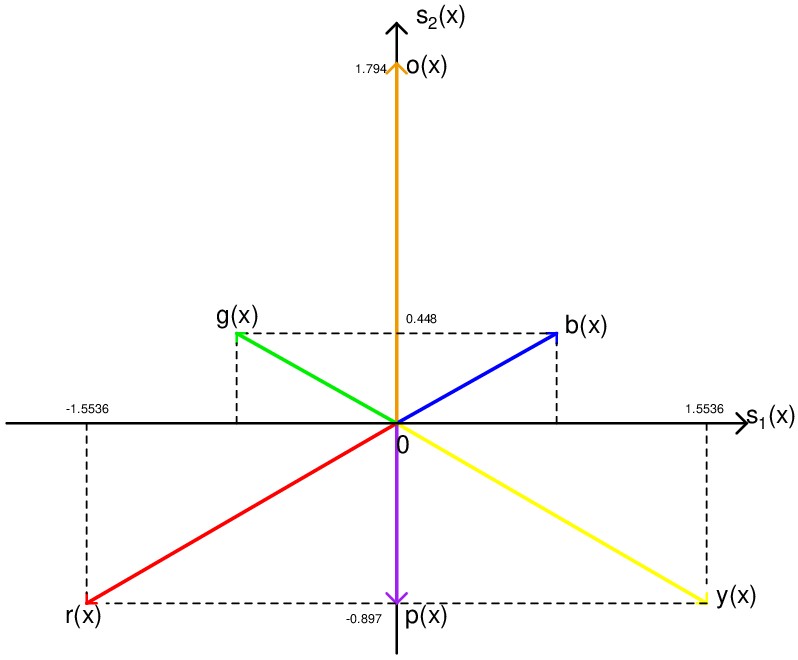
≃\displaystyle\simeq −1.5537⊠s1(x)⊞−0.89701⊠s2(x).\displaystyle-1.5537\boxtimes s_{1}(x)\boxplus-0.89701\boxtimes s_{2}(x)\textrm{.}

The coordinates of all the pmfs mentioned in Example 9.3 are given in the table below and depicted in Figure 2.

Table 2: Coordinates of the pmfs mentioned in Examples 9.3 and 10.12
r⁡(x)r(x) y⁡(x)y(x) o⁡(x)o(x) b⁡(x)b(x) g⁡(x)g(x) p⁡(x)p(x)
s1​(x)s_{1}(x) −1.55367-1.55367 1.553671.55367 00 0.776840.77684 −0.77684-0.77684 00
s2​(x)s_{2}(x) −0.89701-0.89701 −0.89701-0.89701 1.794031.79403 0.448510.44851 0.448510.44851 −0.89701-0.89701
Refer to caption
Figure 2: Plot of the pmfs mentioned in Examples 9.3 and 10.12

11 Relation to the Hilbert space of random variables

The Hilbert space of probability mass functions of finite field-valued random variables might be confused with the Hilbert space of random variables with a finite second order moment which is already well known [31]. However, these two Hilbert spaces are quite different from each other. First of all, the vectors of the former Hilbert space are pmfs of the random variables whereas the vectors of the latter Hilbert space are the random variables themselves. Second, the former Hilbert space is related to the finite-field valued random variables whereas the latter is related to the complex-valued random variables. Finally, the former is meaningful in the Bayesian detection sense whereas the latter is not.

Although this thesis is about the Hilbert space of the pmfs of finite field-valued random variables, it is adequate to summarize the Hilbert space of random variables. The set of complex-valued random variables forms vector space with the usual random variable addition and scaling over ℂ\mathbb{C}. This vector space can be endowed with the following inner product which is nothing but the autocorrelation between two random variables.

<X,Y>=𝐄⁡[X​Y∗]​,<X,Y>=\mathbf{E}\left[XY^{*}\right]\textrm{,} (56)

where XX and YY are two complex-valued random variables and 𝐄[.]\mathbf{E}\left[.\right] denotes the expectation. The set of complex-valued random variables with finite second order moment is complete w.r.t. the norm induced by the inner product above. Therefore, this set forms a Hilbert space over ℂ\mathbb{C} with the usual random variable addition, scaling, and the inner product given in (56). Many important algorithms, such as the Wiener filter, relies upon the orthogonality in this Hilbert space.

Notice that the Hilbert space structure over random variables is constructed over complex-valued random variables. Although it is also possible to construct a similar vector space over the set of finite field-valued random variables, the vector space of finite field-valued random variables does not have an inner product. In other words, the set of 𝔽q\mathbb{F}_{q}-valued random variables forms a vector space with the usual random variable addition and scaling over 𝔽q\mathbb{F}_{q}. On the contrary to complex-valued random variable case, the expected value is not a well defined concept for finite field-valued random variables. Consequently, autocorrelation between two 𝔽q\mathbb{F}_{q}-valued random variables is not well defined either. Therefore, we cannot construct a Hilbert space structure over the set of 𝔽q\mathbb{F}_{q}-valued random variables as we could for the complex valued random variables. If we had a Hilbert space structure over the set of 𝔽q\mathbb{F}_{q}-valued random variables then we would have decoding algorithms for linear channel codes with polynomial complexity.

11.1 Comparison between the convergence of random variables and pmfs

Another possible confusion might arise between the convergence of finite field-valued random variables and the convergence of pmfs of finite field-valued random variables. As explained above expectation is not well defined for finite field-valued random variables. Therefore, convergence in the mean square sense is not well defined for finite field-valued random variables either. On the other hand, convergence modes such as convergence almost everywhere and convergence in probability can still be well defined. However, due to the topological nature of the finite fields these two convergence modes are essentially equivalent. Convergence of a sequence of finite-field-valued random variables in probability is formally defined below.

Definition 11.13.

Convergence of a sequence of finite-field-valued random variables in probability: A sequence of 𝔽q\mathbb{F}_{q}-valued random variables, {Xn}n=1∞\left\{X_{n}\right\}_{n=1}^{\infty}, converges in probability to an 𝔽q\mathbb{F}_{q}-valued random variable XX if and only if for each ϵ>0\epsilon>0 there exist an integer NN such that

n>N⟹Pr{Xn=X}>1−ϵn>N\implies\Pr\{X_{n}=X\}>1-\epsilon (57)

and this convergence is denoted by

limn→∞Pr{Xn=X}=1.\lim_{n\rightarrow\infty}\Pr\{X_{n}=X\}=1\textrm{.} (58)

Convergence of 𝔽q\mathbb{F}_{q}-valued random variables in probability, might be confused with the convergence of pmfs in 𝒫𝔽q\mathcal{P}_{\mathbb{F}_{q}}. The following example aims to clarify the distinction between these two convergences.

Example 11.14.

Let the event space of an experiment Ω\Omega be [0,1]⊂ℝ[0,1]\subset\mathbb{R} and each outcome of the experiment is equally likely, i.e.

Pr{ω≤c}=c,\Pr\{\omega\leq c\}=c\textrm{,} (59)

where ω\omega denotes the outcome of the experiment. A sequence of 𝔽2\mathbb{F}_{2}-valued random variables, {Xn}n=1∞\left\{X_{n}\right\}_{n=1}^{\infty}, are assigned to this experiment as follows.

Xn​(ω)≜{0,ω∈[0,1−2−n]1,ω∈(1−2−n,1]X_{n}(\omega)\triangleq\left\{\begin{array}[]{cc}0,&\omega\in[0,1-2^{-n}]\\ 1,&\omega\in(1-2^{-n},1]\end{array}\right. (60)

Clearly, the sequence {Xn}n=1∞\left\{X_{n}\right\}_{n=1}^{\infty} converges in probability to a random variable XX which is defined as

X≜{0,ω∈[0,1]1,ω∈∅X\triangleq\left\{\begin{array}[]{cl}0,&\omega\in[0,1]\\ 1,&\omega\in\emptyset\end{array}\right. (61)

In other words,

limn→∞Pr{Xn=X}=1.\lim_{n\rightarrow\infty}\Pr\{X_{n}=X\}=1\textrm{.} (62)

Let a sequence {pn​(x)}n=1∞\left\{p_{n}(x)\right\}_{n=1}^{\infty} of pmfs in 𝒫𝔽2\mathcal{P}_{\mathbb{F}_{2}} be defined as

pn​(x)\displaystyle p_{n}(x) ≜\displaystyle\triangleq Pr{Xn=x}\displaystyle\Pr\{X_{n}=x\}
=\displaystyle= {1−2−n,x=02−n,x=1\displaystyle\left\{\begin{array}[]{cc}1-2^{-n},&x=0\\ 2^{-n},&x=1\end{array}\right.

and p⁡(x)p(x) denote Pr{X=x}\Pr\{X=x\}. Due to the basic axioms of probability

p⁡(x)={1,x=00,x=1​.p(x)=\left\{\begin{array}[]{cc}1&,x=0\\ 0&,x=1\end{array}\right.\textrm{.} (66)

It might appear at a first glance that the sequence {pn​(x)}n=1∞\left\{p_{n}(x)\right\}_{n=1}^{\infty} converges to p⁡(x)p(x). However, this would contradict with the completeness of 𝒫𝔽2\mathcal{P}_{\mathbb{F}_{2}} since p⁡(x)∉𝒫𝔽2p(x)\notin\mathcal{P}_{\mathbb{F}_{2}}. The truth is {pn​(x)}n=1∞\left\{p_{n}(x)\right\}_{n=1}^{\infty} is not a Cauchy sequence in 𝒫𝔽2\mathcal{P}_{\mathbb{F}_{2}}. This fact can be shown as follows. For any m>n>0m>n>0

D⁡(pm​(x),pn​(x))\displaystyle D(p_{m}(x),p_{n}(x)) =\displaystyle= ∑i∈𝔽2(log⁡pm​(i)pn​(i))2−1q​(∑i∈𝔽2log⁡pm​(i)pn​(i))2\displaystyle\sqrt{\sum_{i\in\mathbb{F}_{2}}\left(\log\frac{p_{m}(i)}{p_{n}(i)}\right)^{2}-\frac{1}{q}\left(\sum_{i\in\mathbb{F}_{2}}\log\frac{p_{m}(i)}{p_{n}(i)}\right)^{2}}
=\displaystyle= 12​(log⁡pm​(0)pn​(0)+log⁡pn​(1)pm​(1))​.\displaystyle\frac{1}{\sqrt{2}}\left(\log\frac{p_{m}(0)}{p_{n}(0)}+\log\frac{p_{n}(1)}{p_{m}(1)}\right)\textrm{.}

Since pm​(0)>pn​(0)p_{m}(0)>p_{n}(0)

D⁡(pm​(x),pn​(x))\displaystyle D(p_{m}(x),p_{n}(x)) >\displaystyle> 12​(log⁡pn​(1)pm​(1))\displaystyle\frac{1}{\sqrt{2}}\left(\log\frac{p_{n}(1)}{p_{m}(1)}\right) (67)
=\displaystyle= log⁡22​(m−n)​.\displaystyle\frac{\log 2}{\sqrt{2}}(m-n)\textrm{.}

Therefore, {pn​(x)}n=1∞\left\{p_{n}(x)\right\}_{n=1}^{\infty} is not a Cauchy sequence and the limit limn→∞pn​(x)\lim_{n\rightarrow\infty}p_{n}(x) does not exist. This example demonstrates that convergence of a sequence of random variables in probability does not imply the convergence of their pmfs.

12 The Hilbert space of multivariate pmfs

The construction of the Hilbert space on 𝒫𝔽q\mathcal{P}_{\mathbb{F}_{q}} can be applied to the set of multivariate (joint) pmfs as well. Basically, we should replace the indeterminate variable xx in the Hilbert space of pmfs with a vector 𝐱\mathbf{x} while constructing the Hilbert space structure on multivariate pmfs.

Let 𝐗=[X1,X2,…,XN]\mathbf{X}=[X_{1},X_{2},\ldots,X_{N}] be a random vector where XiX_{i} is a 𝔽q\mathbb{F}_{q}-valued random variable. Furthermore, let 𝒫𝔽qN\mathcal{P}_{\mathbb{F}_{q}^{N}} denote the set of all strictly positive pmfs that 𝐗\mathbf{X} might posses, i.e.

𝒫𝔽qN≜{p(𝐱):𝔽qN→(0,1)⊂ℝ,∑𝐱∈𝔽qNp(𝐱)=1}.\mathcal{P}_{\mathbb{F}_{q}^{N}}\triangleq\left\{p(\mathbf{x}):\mathbb{F}_{q}^{N}\rightarrow(0,1)\subset\mathbb{R},\sum_{\mathbf{x}\in\mathbb{F}_{q}^{N}}p(\mathbf{x})=1\right\}\textrm{.} (68)

The addition and scalar multiplication on 𝒫𝔽qN\mathcal{P}_{\mathbb{F}_{q}^{N}} can be defined for any p1​(𝐱),p2​(𝐱),p⁡(𝐱)∈𝒫𝔽qp_{1}(\mathbf{x}),p_{2}(\mathbf{x}),p(\mathbf{x})\in\mathcal{P}_{\mathbb{F}_{q}} and α∈ℝ\alpha\in\mathbb{R} as

p1​(𝐱)⊞p2​(𝐱)\displaystyle p_{1}(\mathbf{x})\boxplus p_{2}(\mathbf{x}) ≜\displaystyle\triangleq 𝒞𝔽qN​{p1​(𝐱)​p2​(𝐱)}\displaystyle\mathcal{C}_{\mathbb{F}_{q}^{N}}\left\{p_{1}(\mathbf{x})p_{2}(\mathbf{x})\right\} (69)
α⊠p⁡(𝐱)\displaystyle\alpha\boxtimes p(\mathbf{x}) ≜\displaystyle\triangleq 𝒞𝔽qN​{(p⁡(𝐱))α}\displaystyle\mathcal{C}_{\mathbb{F}_{q}^{N}}\left\{(p(\mathbf{x}))^{\alpha}\right\} (70)

The normalization operator in the multivariate case, which is denoted by 𝒞𝔽qN{.}\mathcal{C}_{\mathbb{F}_{q}^{N}}\left\{.\right\} above, maps any strictly positive function of 𝔽qN\mathbb{F}_{q}^{N}, α⁡(𝐱)\alpha(\mathbf{x}), to a pmf in 𝒫𝔽qN\mathcal{P}_{\mathbb{F}_{q}^{N}} as follows.

𝒞𝔽qN​{α⁡(𝐱)}≜α⁡(𝐱)∑𝐢∈𝔽qNα⁡(𝐢)\mathcal{C}_{\mathbb{F}_{q}^{N}}\left\{\alpha(\mathbf{x})\right\}\triangleq\frac{\alpha(\mathbf{x})}{\sum_{\mathbf{i}\in\mathbb{F}_{q}^{N}}\alpha(\mathbf{i})} (71)

Similar to the univariate case, 𝒫𝔽qN\mathcal{P}_{\mathbb{F}_{q}^{N}} together with the ⊞\boxplus and ⊠\boxtimes operations forms a vector space over ℝ\mathbb{R}.

The analogue of the mapping ℒ{.}\mathcal{L}\left\{.\right\} in the multivariate case is denoted by ℒN{.}\mathcal{L}_{N}\left\{.\right\} and maps the pmfs in 𝒫𝔽qN\mathcal{P}_{\mathbb{F}_{q}^{N}} to ℝ(qN)\mathbb{R}^{(q^{N})}. Before giving the definition of ℒN{.}\mathcal{L}_{N}\left\{.\right\} we need to establish a one-to-one matching between the vectors in 𝔽qN\mathbb{F}_{q}^{N} and the canonical basis vectors of ℝ(qN)\mathbb{R}^{(q^{N})}. We can do this matching since 𝔽qN\mathbb{F}_{q}^{N} contains qNq^{N} vectors which is equal to the dimension of ℝ(qN)\mathbb{R}^{(q^{N})}. Since the mapping ℒN{.}\mathcal{L}_{N}\left\{.\right\} is going to be employed in borrowing the inner product in ℝ(qN)\mathbb{R}^{(q^{N})} the order of matching is not important.

Using this matching ℒN{.}\mathcal{L}_{N}\left\{.\right\} is defined as

ℒN​{p⁡(𝐱)}:𝒫𝔽qN→ℝ(qN)≜∑𝐢∈𝔽qN(log⁡p⁡(𝐢)−1qN​∑𝐣∈𝔽qNlog⁡p⁡(𝐣))​𝐞𝐢​,\mathcal{L}_{N}\left\{p(\mathbf{x})\right\}:\mathcal{P}_{\mathbb{F}_{q}^{N}}\rightarrow\mathbb{R}^{(q^{N})}\triangleq\sum_{\mathbf{i}\in\mathbb{F}_{q}^{N}}\left(\log p(\mathbf{i})-\frac{1}{q^{N}}\sum_{\mathbf{j}\in\mathbb{F}_{q}^{N}}\log p(\mathbf{j})\right)\mathbf{e}_{\mathbf{i}}\textrm{,} (72)

where 𝐞𝐢\mathbf{e}_{\mathbf{i}} denotes the canonical basis vector of ℝ(qN)\mathbb{R}^{(q^{N})} matched to 𝐢∈𝔽qN\mathbf{i}\in\mathbb{F}_{q}^{N}. ℒN{.}\mathcal{L}_{N}\left\{.\right\} is a linear and injective mapping as ℒ{.}\mathcal{L}\left\{.\right\}. Then the inner product of any two p⁡(𝐱),r⁡(𝐱)∈𝒫𝔽qNp(\mathbf{x}),r(\mathbf{x})\in\mathcal{P}_{\mathbb{F}_{q}^{N}} becomes

<p⁡(𝐱),r⁡(𝐱)>\displaystyle<p(\mathbf{x}),r(\mathbf{x})> ≜\displaystyle\triangleq <ℒN​{p⁡(𝐱)},ℒN​{r⁡(𝐱)}>ℝ(qN)\displaystyle<\mathcal{L}_{N}\left\{p(\mathbf{x})\right\},\mathcal{L}_{N}\left\{r(\mathbf{x})\right\}>_{\mathbb{R}^{(q^{N})}} (73)
=\displaystyle= ∑𝐢∈𝔽qNlog⁡p⁡(𝐢)​log⁡r⁡(𝐢)−1qN​(∑𝐢∈𝔽qNlog⁡p⁡(𝐢))​(∑𝐢∈𝔽qNlog⁡r⁡(𝐢))​.\displaystyle\sum_{\mathbf{i}\in\mathbb{F}_{q}^{N}}\log p(\mathbf{i})\log r(\mathbf{i})-\frac{1}{q^{N}}\left(\sum_{\mathbf{i}\in\mathbb{F}_{q}^{N}}\log p(\mathbf{i})\right)\left(\sum_{\mathbf{i}\in\mathbb{F}_{q}^{N}}\log r(\mathbf{i})\right)\textrm{.} (74)

The definition of inner product makes 𝒫𝔽qN\mathcal{P}_{\mathbb{F}_{q}^{N}} an inner product space. Since 𝒫𝔽qN\mathcal{P}_{\mathbb{F}_{q}^{N}} is definitely finite dimensional it is also a Hilbert space.

The pseudo inverse of ℒN{.}\mathcal{L}_{N}\left\{.\right\} is

ℒN+​{𝐩}​(𝐱):ℝ(qN)→𝒫𝔽qN≜𝒞𝔽qN​{exp⁡(−12​‖𝐩−𝐬N​(𝐱)‖2)}​,\mathcal{L}_{N}^{+}\left\{\mathbf{p}\right\}(\mathbf{x}):\mathbb{R}^{(q^{N})}\rightarrow\mathcal{P}_{\mathbb{F}_{q}^{N}}\triangleq\mathcal{C}_{\mathbb{F}_{q}^{N}}\left\{\exp\left(-\frac{1}{2}\left\|\mathbf{p}-\mathbf{s}_{N}(\mathbf{x})\right\|^{2}\right)\right\}\textrm{,} (75)

where 𝐬N​(𝐱)\mathbf{s}_{N}(\mathbf{x}) is

𝐬N​(𝐱)≜𝐞𝐱−1qN​𝟏​.\mathbf{s}_{N}(\mathbf{x})\triangleq\mathbf{e}_{\mathbf{x}}-\frac{1}{q^{N}}\mathbf{1}\textrm{.} (76)

The vector 𝟏\mathbf{1} above denotes the all one vector in ℝ(qN)\mathbb{R}^{(q^{N})}. Similar to the univariate case it can be shown that ℒN+{.}(𝐱)\mathcal{L}_{N}^{+}\left\{.\right\}(\mathbf{x}) satisfies

ℒN+​{ℒN​{p⁡(𝐱)}}​(𝐱)=p⁡(𝐱)\displaystyle\mathcal{L}_{N}^{+}\left\{\mathcal{L}_{N}\left\{p(\mathbf{x})\right\}\right\}(\mathbf{x})=p(\mathbf{x}) ∀p⁡(𝐱)∈𝒫𝔽q\displaystyle\quad\forall p(\mathbf{x})\in\mathcal{P}_{\mathbb{F}_{q}} (77)
ℒN​{ℒN+​{𝐩}​(𝐱)}=𝐩\displaystyle\mathcal{L}_{N}\left\{\mathcal{L}_{N}^{+}\left\{\mathbf{p}\right\}(\mathbf{x})\right\}=\mathbf{p} ∀𝐩∈𝟏⟂⊂ℝ(qN)​.\displaystyle\quad\forall\mathbf{p}\in\mathbf{1}^{\perp}\subset\mathbb{R}^{(q^{N})}\textrm{.} (78)

Consequently,

im⁡{ℒN}=𝟏⟂⊂ℝ(qN)\mathrm{im}\left\{\mathcal{L}_{N}\right\}=\mathbf{1}^{\perp}\subset\mathbb{R}^{(q^{N})} (79)
Theorem 12.15.

𝒫𝔽qN\mathcal{P}_{\mathbb{F}_{q}^{N}} is a qN−1q^{N}-1 dimensional Hilbert space, i.e.

dim𝒫𝔽qN=qN−1​.\dim\mathcal{P}_{\mathbb{F}_{q}^{N}}=q^{N}-1\textrm{.} (80)
Proof 12.16.

Due to the rank-nullity theorem in linear algebra

dim𝒫𝔽qN\displaystyle\dim\mathcal{P}_{\mathbb{F}_{q}^{N}} =\displaystyle= dimker⁡{ℒN}+dimim⁡{ℒN}\displaystyle\dim\mathrm{ker}\left\{\mathcal{L}_{N}\right\}+\dim\mathrm{im}\left\{\mathcal{L}_{N}\right\} (81)
=\displaystyle= qN−1​.\displaystyle q^{N}-1\textrm{.} (82)

As a minor consequence of this theorem we can conclude that 𝒫𝔽qN\mathcal{P}_{\mathbb{F}_{q}^{N}} is isomorphic to 𝒫𝔽qN\mathcal{P}_{\mathbb{F}_{q^{N}}}. This is a quite expected result since 𝔽qN\mathbb{F}_{q}^{N} is isomorphic to 𝔽qN\mathbb{F}_{q^{N}}.

Chapter 3 THE CANONICAL FACTORIZATION OF
MULTIVARIATE PROBABILITY MASS FUNCTIONS

13 Introduction

The factorization of a multivariate pmf is important in many aspects. For instance, the conditional dependence of the random variables distributed by a pmf can be determined by how the pmf factors. Existence of low complexity maximization and marginalization algorithms for a multivariate pmf, such as Viterbi and BCJR, also depends on the factorization of the pmf. A very special factorization of multivariate pmfs which we call as the canonical factorization is introduced in this chapter.

This chapter begins with representing the factorization of a pmf in 𝒫𝔽qN\mathcal{P}_{\mathbb{F}_{q}^{N}}. Then we introduce the soft parity check constraints using which we decompose 𝒫𝔽qN\mathcal{P}_{\mathbb{F}_{q}^{N}} into orthogonal subspaces. Finally, we obtain the canonical factorization of pmfs as the projection of pmfs onto these subspaces.

14 Representing the factorization of pmfs

The Hilbert space 𝒫𝔽qN\mathcal{P}_{\mathbb{F}_{q}^{N}} provides a suitable environment for analyzing the factorization of multivariate pmfs. Suppose that a pmf in 𝒫𝔽qN\mathcal{P}_{\mathbb{F}_{q}^{N}} can be factored as

p⁡(𝐱)=∏i=1Kϕi​(𝐱)​.p(\mathbf{x})=\prod_{i=1}^{K}\phi_{i}(\mathbf{x})\textrm{.} (83)

Each ϕi​(𝐱)\phi_{i}(\mathbf{x}) function appearing above may be called a factor function, a local function, a constraint, or an interaction. The factor functions are not necessarily pmfs but they can be assumed to be positive. Hence, we can obtain a pmf in 𝒫𝔽q\mathcal{P}_{\mathbb{F}_{q}} by scaling the factor functions as in

ri​(𝐱)\displaystyle r_{i}(\mathbf{x}) =\displaystyle= 𝒞𝔽qN​{ϕi​(𝐱)}\displaystyle\mathcal{C}_{\mathbb{F}_{q}^{N}}\left\{\phi_{i}(\mathbf{x})\right\} (84)
=\displaystyle= 1γi​ϕi​(𝐱)​,\displaystyle\frac{1}{\gamma_{i}}\phi_{i}(\mathbf{x})\textrm{,} (85)

where γi=∑𝐢∈𝔽qNϕi​(𝐱)\gamma_{i}=\sum_{\mathbf{i}\in\mathbb{F}_{q}^{N}}\phi_{i}(\mathbf{x}). After this normalization the factorization in (83) becomes

p⁡(𝐱)\displaystyle p(\mathbf{x}) =\displaystyle= ∏i=1Kγi​ri​(𝐱)\displaystyle\prod_{i=1}^{K}\gamma_{i}r_{i}(\mathbf{x}) (86)
=\displaystyle= 𝒞𝔽qN​{∏i=1Kri​(𝐱)}​,\displaystyle\mathcal{C}_{\mathbb{F}_{q}^{N}}\left\{\prod_{i=1}^{K}r_{i}(\mathbf{x})\right\}\textrm{,} (87)

which can be represented using the addition in 𝒫𝔽q\mathcal{P}_{\mathbb{F}_{q}} as

p⁡(𝐱)=∑i=1K⊞​ri​(𝐱)​.p(\mathbf{x})=\sideset{{}^{\boxplus}}{}{\sum}_{i=1}^{K}r_{i}(\mathbf{x})\textrm{.} (88)

This representation suggests that a multivariate pmf in 𝒫𝔽qN\mathcal{P}_{\mathbb{F}_{q}^{N}} can be factored by expressing it as a linear combination of some basis vectors (pmfs) in 𝒫𝔽qN\mathcal{P}_{\mathbb{F}_{q}^{N}}. If these basis pmfs are chosen to be orthogonal then we can employ the inner product on 𝒫𝔽qN\mathcal{P}_{\mathbb{F}_{q}^{N}} to determine the expansion coefficients. However, the basis pmfs should be selected in such a way that the resulting factorization becomes useful.

We know from the literature on the sum-product algorithm [1, 2, 6, 7] and Markov random fields [17, 18, 19, 20] that the factorization of p⁡(𝐱)p(\mathbf{x}) given in (83) is useful if the factor functions on the right hand side of (83) are local. A factor function of p⁡(𝐱)p(\mathbf{x}) is said to be local if it depends on some but not all of the components of the argument vector 𝐱\mathbf{x}. Therefore, the basis functions mentioned in the paragraph above should also be selected to be as local as possible.

15 The multivariate pmfs that can be expressed as a function of a linear
combination of their arguments

In this section we propose a special type of multivariate pmfs which will serve as basis vectors to obtain a factorization of pmfs in 𝒫𝔽q\mathcal{P}_{\mathbb{F}_{q}}. We show in the next chapter that the factorization obtained using these basis pmfs is quite useful. These basis pmfs are inspired by the parity check relations in 𝔽q\mathbb{F}_{q}. Suppose that the components of an 𝔽qN\mathbb{F}_{q}^{N}-valued random vector 𝐗=[X1,X2,…,XN]\mathbf{X}=[X_{1},X_{2},\ldots,X_{N}] satisfy the following parity check relation

a1​X1+a2​X2+…+aN​XN=0​,a_{1}X_{1}+a_{2}X_{2}+\ldots+a_{N}X_{N}=0\textrm{,} (89)

where aia_{i} is a constant in 𝔽q\mathbb{F}_{q}. If all configurations satisfying this relation are assumed to be equiprobable then the joint pmf of 𝐗\mathbf{X}, which is denoted by p⁡(𝐱)p(\mathbf{x}), is

p⁡(𝐱)={1qN−1,∑i=1Nai​xi=00,otherwise​.p(\mathbf{x})=\left\{\begin{array}[]{cc}\frac{1}{q^{N-1}},&\sum_{i=1}^{N}a_{i}x_{i}=0\\ 0,&\textrm{otherwise}\end{array}\right.\textrm{.} (90)

This pmf can be expressed in a more compact form as

p⁡(𝐱)\displaystyle p(\mathbf{x}) =\displaystyle= 1qN−1​δ​(𝐚𝐱T)\displaystyle\frac{1}{q^{N-1}}\delta(\mathbf{a}\mathbf{x}^{T}) (91)
=\displaystyle= 𝒞𝔽qN​{δ⁡(𝐚𝐱T)}​,\displaystyle\mathcal{C}_{\mathbb{F}_{q}^{N}}\left\{\delta(\mathbf{a}\mathbf{x}^{T})\right\}\textrm{,} (92)

where 𝐚\mathbf{a} is [a1,a2,…,aN][a_{1},a_{2},\ldots,a_{N}] and δ(.)\delta(.) denotes the Kronecker delta.

The multivariate pmfs which can be expressed in the form as in (92) are called parity check or zero-sum constraints. A parity check constraint depends only on the variables which have nonzero coefficients associated with them. Hence, they posses local function properties as we desire from a basis pmf. Therefore, parity check constraints could be good candidates for being basis pmfs if they were elements of 𝒫𝔽qN\mathcal{P}_{\mathbb{F}_{q}^{N}}. However, parity check constraints are not elements of 𝒫𝔽qN\mathcal{P}_{\mathbb{F}_{q}^{N}}, since their value is zero for the configurations which do not satisfy the parity check relation.

We can obtained a “softened” version of the parity check constraints as follows. Suppose that the components of the random vector 𝐗\mathbf{X} satisfy the following relation instead of (89)

a1​X1+a2​X2+…+aN​XN=U​,a_{1}X_{1}+a_{2}X_{2}+\ldots+a_{N}X_{N}=U\textrm{,} (93)

where UU is an 𝔽q\mathbb{F}_{q}-valued random variable distributed with an r⁡(u)∈𝒫𝔽qr(u)\in\mathcal{P}_{\mathbb{F}_{q}}. If all configurations resulting with the same value of UU are assumed to be equiprobable then joint pmf of 𝐗\mathbf{X} in this case becomes

p⁡(𝐱)\displaystyle p(\mathbf{x}) =\displaystyle= {1qN−1​r​(0),∑i=1Nai​xi=01qN−1​r​(1),∑i=1Nai​xi=1⋮⋮1qN−1​r​(q−1),∑i=1Nai​xi=q−1\displaystyle\left\{\begin{array}[]{cl}\frac{1}{q^{N-1}}r(0),&\sum_{i=1}^{N}a_{i}x_{i}=0\\ \frac{1}{q^{N-1}}r(1),&\sum_{i=1}^{N}a_{i}x_{i}=1\\ \vdots&\vdots\\ \frac{1}{q^{N-1}}r(q-1),&\sum_{i=1}^{N}a_{i}x_{i}=q-1\end{array}\right.

which can be expressed in a more compact form as

p⁡(𝐱)\displaystyle p(\mathbf{x}) =\displaystyle= 1qN−1​r​(𝐚𝐱T)\displaystyle\frac{1}{q^{N-1}}r(\mathbf{a}\mathbf{x}^{T}) (99)
=\displaystyle= 𝒞𝔽qN​{r⁡(𝐚𝐱T)}​.\displaystyle\mathcal{C}_{\mathbb{F}_{q}^{N}}\left\{r(\mathbf{a}\mathbf{x}^{T})\right\}\textrm{.} (100)
Definition 15.1.

A multivariate pmf p⁡(𝐱)p(\mathbf{x}) in 𝒫𝔽qN\mathcal{P}_{\mathbb{F}_{q}^{N}} is called a soft parity check (SPC) constraint if there exist a r⁡(x)∈𝒫𝔽qr(x)\in\mathcal{P}_{\mathbb{F}_{q}} and a vector 𝐚=[a0,a1,…,aN−1]∈𝔽qN\mathbf{a}=[a_{0},a_{1},\ldots,a_{N-1}]\in\mathbb{F}_{q}^{N} such that

p⁡(𝐱)\displaystyle p(\mathbf{x}) =\displaystyle= 𝒞𝔽qN​{r⁡(𝐚𝐱T)}​.\displaystyle\mathcal{C}_{\mathbb{F}_{q}^{N}}\left\{r(\mathbf{a}\mathbf{x}^{T})\right\}\textrm{.} (101)

The vector 𝐚\mathbf{a} is called the parity check coefficient vector of the SPC constraint p⁡(𝐱)p(\mathbf{x}).

The difference between parity check and SPC constraint is the distribution of the weighted sum of the random variables X0X_{0}, X1X_{1}, …\ldots, XN−1X_{N-1}, which is denoted by UU in (93). UU is distributed with δ⁡(u)\delta(u) in the parity check case whereas it is distributed with a r⁡(u)r(u) in 𝒫𝔽q\mathcal{P}_{\mathbb{F}_{q}} in the SPC constraint case. The term “soft” arises from the fact that the weighted sum can take all values with some probability rather than guaranteed to be zero. Therefore, unlike parity check constraints SPC constraints are in 𝒫𝔽qN\mathcal{P}_{\mathbb{F}_{q}^{N}}, since all configurations have nonzero probabilities.

Example 15.2.

Let two pmfs in 𝒫𝔽32\mathcal{P}_{\mathbb{F}_{3}^{2}} are given with a slight abuse of notation as

p1​(x0,x1)\displaystyle p_{1}(x_{0},x_{1}) =\displaystyle= 130​[361613136]\displaystyle\frac{1}{30}\left[\begin{array}[]{ccc}3&6&1\\ 6&1&3\\ 1&3&6\end{array}\right]
p2​(x0,x1)\displaystyle p_{2}(x_{0},x_{1}) =\displaystyle= 1157​[123011064812830]​,\displaystyle\frac{1}{157}\left[\begin{array}[]{ccc}12&30&1\\ 10&6&48\\ 12&8&30\end{array}\right]\textrm{,}

where pk​(x0=i,x1=j)p_{k}(x_{0}=i,x_{1}=j) is given by the entry in the (i+1)t​h(i+1)^{th} row and the (j+1)t​h(j+1)^{th} column of the corresponding matrix.

Notice that p1​(x0,x1)p_{1}(x_{0},x_{1}) can be expressed as

p1​(x0,x1)\displaystyle p_{1}(x_{0},x_{1}) =\displaystyle= 13​r​(x0+x1)\displaystyle\frac{1}{3}r(x_{0}+x_{1})
=\displaystyle= 𝒞𝔽32​{r⁡(x0+x1)}\displaystyle\mathcal{C}_{\mathbb{F}_{3}^{2}}\left\{r(x_{0}+x_{1})\right\}

where r⁡(x)∈𝒫𝔽3Nr(x)\in\mathcal{P}_{\mathbb{F}_{3}^{N}} is

r⁡(x)={0.3,x=00.6,x=10.1x=1​.r(x)=\left\{\begin{array}[]{cc}0.3,&x=0\\ 0.6,&x=1\\ 0.1&x=1\end{array}\right.\textrm{.}

Therefore, p1​(x0,x1)p_{1}(x_{0},x_{1}) is an SPC constraint with parity check coefficient vector [1,1][1,1]. On the other hand, we cannot find a similar expression for p2​(x0,x1)p_{2}(x_{0},x_{1}). Hence, p2​(x0,x1)p_{2}(x_{0},x_{1}) is not an SPC constraint.

Notice that we exploited the field structure of 𝔽q\mathbb{F}_{q} in the discussion above. Parity check relations could also be described in finite rings but the number of configurations satisfying a parity check relation depends on the parity check coefficients in a finite ring. Therefore, the SPC constraints in a finite ring would not be in a nice form as above.

In the rest of this chapter we are going to show that SPC constraints form a complete set of orthogonal basis functions for 𝒫𝔽qN\mathcal{P}_{\mathbb{F}_{q}^{N}}. The first step of this process is the following lemma which analyzes the inner product of two SPC constraints.

Lemma 15.3.

Inner product of two SPC constraints: Let p1​(𝐱),p2​(𝐱)∈𝒫𝔽qNp_{1}(\mathbf{x}),p_{2}(\mathbf{x})\in\mathcal{P}_{\mathbb{F}_{q}^{N}} are two SPC constraints such that

p1​(𝐱)\displaystyle p_{1}(\mathbf{x}) =\displaystyle= 𝒞𝔽qN​{r1​(𝐚𝐱T)}\displaystyle\mathcal{C}_{\mathbb{F}_{q}^{N}}\left\{r_{1}(\mathbf{a}\mathbf{x}^{T})\right\} (110)
p2​(𝐱)\displaystyle p_{2}(\mathbf{x}) =\displaystyle= 𝒞𝔽qN​{r2​(𝐛𝐱T)}​,\displaystyle\mathcal{C}_{\mathbb{F}_{q}^{N}}\left\{r_{2}(\mathbf{b}\mathbf{x}^{T})\right\}\textrm{,}

where r1​(x),r2​(x)∈𝒫𝔽qr_{1}(x),r_{2}(x)\in\mathcal{P}_{\mathbb{F}_{q}}. If 𝐚\mathbf{a} and 𝐛\mathbf{b} are both nonzero vectors in 𝔽qN\mathbb{F}_{q}^{N} then

<p1(𝐱),p2(𝐱)>={qN−1​<r1​(x),r2​(α​x)>,∃α∈𝔽q:𝐛=α​𝐚0,otherwise<p_{1}(\mathbf{x}),p_{2}(\mathbf{x})>=\left\{\begin{array}[]{cc}q^{N-1}<r_{1}(x),r_{2}(\alpha x)>,&\exists\alpha\in\mathbb{F}_{q}:\mathbf{b}=\alpha\mathbf{a}\\ 0,&\textrm{otherwise}\end{array}\right. (111)

The proof of this lemma is given in Appendix 9.B.1.

16 Orthogonal Subspace Decomposition of 𝒫𝔽qN\mathcal{P}_{\mathbb{F}_{q}^{N}}

Generating an SPC constraint in 𝒫𝔽qN\mathcal{P}_{\mathbb{F}_{q}^{N}} based on a pmf in 𝒫𝔽q\mathcal{P}_{\mathbb{F}_{q}} and a parity check coefficient vector 𝐚\mathbf{a} can be viewed as a mapping from 𝒫𝔽q\mathcal{P}_{\mathbb{F}_{q}} to 𝒫𝔽qN\mathcal{P}_{\mathbb{F}_{q}^{N}} parameterized on 𝐚\mathbf{a} as given below.

𝒮𝐚​{p⁡(x)}:𝒫𝔽q→𝒫𝔽qN≜𝒞𝔽qN​{p⁡(𝐚𝐱T)}\mathcal{S}_{\mathbf{a}}\left\{p(x)\right\}:\mathcal{P}_{\mathbb{F}_{q}}\rightarrow\mathcal{P}_{\mathbb{F}_{q}^{N}}\triangleq\mathcal{C}_{\mathbb{F}_{q}^{N}}\left\{p(\mathbf{a}\mathbf{x}^{T})\right\} (112)

Any SPC constraint with parity check coefficient vector 𝐚\mathbf{a} is in im​{𝒮𝐚}\mathrm{im}\left\{\mathcal{S}_{\mathbf{a}}\right\}. The first of the following pair of lemmas states that im​{𝒮𝐚}\mathrm{im}\left\{\mathcal{S}_{\mathbf{a}}\right\} is a subspace of 𝒫𝔽qN\mathcal{P}_{\mathbb{F}_{q}^{N}} and the second one investigates the relation between two such subspaces.

Lemma 16.4.

For any nonzero parity check coefficient vector 𝐚\mathbf{a} in 𝔽qN\mathbb{F}_{q}^{N}, im​{𝒮𝐚}\mathrm{im}\left\{\mathcal{S}_{\mathbf{a}}\right\} is a q−1q-1 dimensional subspace of 𝒫𝔽qN\mathcal{P}_{\mathbb{F}_{q}^{N}}.

Lemma 16.5.

For any two nonzero parity check coefficient vectors 𝐚,𝐛∈𝔽qN\mathbf{a},\mathbf{b}\in\mathbb{F}_{q}^{N}

∃α∈𝔽q:𝐚=α​𝐛\displaystyle\exists\alpha\in\mathbb{F}_{q}:\mathbf{a}=\alpha\mathbf{b} ⟹\displaystyle\implies im⁡{𝒮𝐚}=im⁡{𝒮𝐛}\displaystyle\mathrm{im}\left\{\mathcal{S}_{\mathbf{a}}\right\}=\mathrm{im}\left\{\mathcal{S}_{\mathbf{b}}\right\} (113)
∄α∈𝔽q:𝐚=α𝐛\displaystyle\nexists\alpha\in\mathbb{F}_{q}:\mathbf{a}=\alpha\mathbf{b} ⟹\displaystyle\implies im⁡{𝒮𝐚}⟂im⁡{𝒮𝐛}\displaystyle\mathrm{im}\left\{\mathcal{S}_{\mathbf{a}}\right\}\perp\mathrm{im}\left\{\mathcal{S}_{\mathbf{b}}\right\} (114)

The proofs of this lemmas are given in Appendix 9.B.2 and Appendix 9.B.3 respectively.

Lemma 16.5 suggests that 𝒫𝔽qN\mathcal{P}_{\mathbb{F}_{q}^{N}} can be decomposed into orthogonal subspaces by using a sufficient number of parity check coefficient vectors which are all pairwise linearly independent. Fortunately, we can borrow such a set of parity check coefficient vectors from coding theory as explained by the following theorem.

Theorem 16.6.

There exists a set ℋ\mathcal{H} of pairwise linearly independent parity check vectors in 𝔽q\mathbb{F}_{q} of length NN such that

⨁𝐚∈ℋim⁡{𝒮𝐚}=𝒫𝔽qN​.\bigoplus_{\mathbf{a}\in\mathcal{H}}\mathrm{im}\left\{\mathcal{S}_{\mathbf{a}}\right\}=\mathcal{P}_{\mathbb{F}_{q}^{N}}\textrm{.} (115)

where ⨁\bigoplus denotes orthogonal direct summation.

Proof 16.7.

For all nonzero 𝐚\mathbf{a}, im​{𝒮𝐚}\mathrm{im}\left\{\mathcal{S}_{\mathbf{a}}\right\} is a subspace of 𝒫𝔽qN\mathcal{P}_{\mathbb{F}_{q}^{N}}. Orthogonal direct sum of subspaces is again a subspace of 𝒫𝔽qN\mathcal{P}_{\mathbb{F}_{q}^{N}}. Therefore, we can complete the proof by finding an ℋ\mathcal{H} which makes

dim⨁𝐚∈ℋim⁡{𝒮𝐚}=dim𝒫𝔽qN​.\dim\bigoplus_{\mathbf{a}\in\mathcal{H}}\mathrm{im}\left\{\mathcal{S}_{\mathbf{a}}\right\}=\dim\mathcal{P}_{\mathbb{F}_{q}^{N}}\textrm{.} (116)

Let the elements of ℋ\mathcal{H} be selected by transposing the columns of the parity check matrix of the Hamming code in 𝔽q\mathbb{F}_{q} with NN rows. It is known from coding theory that the parity check matrix of such a Hamming code consists of qN−1q−1\frac{q^{N}-1}{q-1} columns all of which are pairwise linearly independent [11]. Therefore, ℋ\mathcal{H} contains qN−1q−1\frac{q^{N}-1}{q-1} pairwise linearly independent vectors. Since these vectors are pairwise linearly independent, for any 𝐚,𝐛∈ℋ\mathbf{a},\mathbf{b}\in\mathcal{H}

im⁡{𝒮𝐚}⟂im⁡{𝒮𝐛}\mathrm{im}\left\{\mathcal{S}_{\mathbf{a}}\right\}\perp\mathrm{im}\left\{\mathcal{S}_{\mathbf{b}}\right\} (117)

due to Lemma 16.5. Hence,

dim⨁𝐚∈ℋim⁡{𝒮𝐚}=∑𝐚∈ℋdimim⁡{𝒮𝐚}​,\dim\bigoplus_{\mathbf{a}\in\mathcal{H}}\mathrm{im}\left\{\mathcal{S}_{\mathbf{a}}\right\}=\sum_{\mathbf{a}\in\mathcal{H}}\dim\mathrm{im}\left\{\mathcal{S}_{\mathbf{a}}\right\}\textrm{,} (118)

since these subspace are all orthogonal. im​{𝒮𝐚}\mathrm{im}\left\{\mathcal{S}_{\mathbf{a}}\right\} is a q−1q-1 dimensional subspace due to Lemma 16.4. Therefore,

dim⨁𝐚∈ℋim⁡{𝒮𝐚}\displaystyle\dim\bigoplus_{\mathbf{a}\in\mathcal{H}}\mathrm{im}\left\{\mathcal{S}_{\mathbf{a}}\right\} =\displaystyle= ∑𝐚∈ℋ(q−1)\displaystyle\sum_{\mathbf{a}\in\mathcal{H}}(q-1) (119)
=\displaystyle= |ℋ|​(q−1)\displaystyle|\mathcal{H}|(q-1)
=\displaystyle= qN−1\displaystyle q^{N}-1
=\displaystyle= dim𝒫𝔽qN​,\displaystyle\dim\mathcal{P}_{\mathbb{F}_{q}^{N}}\textrm{,}

which completes the proof.

17 The Canonical Factorization

Corollary 17.8.

(The fundamental result of the thesis:) Any multivariate pmf in 𝒫𝔽qN\mathcal{P}_{\mathbb{F}_{q}^{N}} can be expressed as a product of functions that depend on a linear combination of their arguments.

Proof 17.9.

Let ℋ\mathcal{H} be set of parity check vectors satisfying (115), existence of which is guaranteed by Theorem 16.6. Let the vectors in ℋ\mathcal{H} be enumerated as 𝐚1,𝐚2,…,𝐚|ℋ|\mathbf{a}_{1},\mathbf{a}_{2},\ldots,\mathbf{a}_{|\mathcal{H}|}. Then any p⁡(𝐱)∈𝒫𝔽qNp(\mathbf{x})\in\mathcal{P}_{\mathbb{F}_{q}^{N}} can be expressed as

p⁡(𝐱)=∑i=1|ℋ|⊞​pi​(𝐱)p(\mathbf{x})=\sideset{{}^{\boxplus}}{}{\sum}_{i=1}^{|\mathcal{H}|}p_{i}(\mathbf{x}) (120)

where pi​(𝐱)p_{i}(\mathbf{x}) is the projection of p⁡(𝐱)p(\mathbf{x}) onto im​{𝒮𝐚i}\mathrm{im}\left\{\mathcal{S}_{\mathbf{a}_{i}}\right\}. Since pi​(𝐱)p_{i}(\mathbf{x}) is in im​{𝒮𝐚i}\mathrm{im}\left\{\mathcal{S}_{\mathbf{a}_{i}}\right\}, there exist an ri​(x)∈𝒫𝔽qr_{i}(x)\in\mathcal{P}_{\mathbb{F}_{q}} such that

pi​(𝐱)=𝒞𝔽qN​{ri​(𝐚i​𝐱T)}​.p_{i}(\mathbf{x})=\mathcal{C}_{\mathbb{F}_{q}^{N}}\left\{r_{i}(\mathbf{a}_{i}\mathbf{x}^{T})\right\}\textrm{.} (121)

Then p⁡(𝐱)p(\mathbf{x}) can be expressed as

p⁡(𝐱)=∑i=1|ℋ|⊞​𝒞𝔽qN​{ri​(𝐚i​𝐱T)}​.p(\mathbf{x})=\sideset{{}^{\boxplus}}{}{\sum}_{i=1}^{|\mathcal{H}|}\mathcal{C}_{\mathbb{F}_{q}^{N}}\left\{r_{i}(\mathbf{a}_{i}\mathbf{x}^{T})\right\}\textrm{.} (122)

Employing the definition of addition in 𝒫𝔽qN\mathcal{P}_{\mathbb{F}_{q}^{N}} yields the desired factorization.

p⁡(𝐱)\displaystyle p(\mathbf{x}) =\displaystyle= 𝒞𝔽qN​{∏i=1|ℋ|ri​(𝐚i​𝐱T)}\displaystyle\mathcal{C}_{\mathbb{F}_{q}^{N}}\left\{\prod_{i=1}^{|\mathcal{H}|}r_{i}(\mathbf{a}_{i}\mathbf{x}^{T})\right\} (123)
=\displaystyle= 1γ​∏i=1|ℋ|ri​(𝐚i​𝐱T)​,\displaystyle\frac{1}{\gamma}\prod_{i=1}^{|\mathcal{H}|}r_{i}(\mathbf{a}_{i}\mathbf{x}^{T})\textrm{,} (124)

where γ\gamma is equal to ∑∀𝐢∈𝔽qN∏i=1|ℋ|ri​(𝐚i​𝐱T)\sum_{\forall\mathbf{i}\in\mathbb{F}_{q}^{N}}\prod_{i=1}^{|\mathcal{H}|}r_{i}(\mathbf{a}_{i}\mathbf{x}^{T}).

Definition 17.10.

The canonical factorization: A factorization of a multivariate pmf is called the canonical factorization of the pmf if all factor functions are SPC factors and parity check coefficient vectors of all SPC factors are pairwise linearly independent.

The canonical factorization of a multivariate pmf in 𝒫𝔽qN\mathcal{P}_{\mathbb{F}_{q}^{N}} can be obtained by projecting the pmf onto the subspaces im​{𝒮𝐚i}\mathrm{im}\left\{\mathcal{S}_{\mathbf{a}_{i}}\right\} for 𝐚i∈ℋ\mathbf{a}_{i}\in\mathcal{H}. In order to compute this projection a set of orthonormal basis pmfs for im​{𝒮𝐚i}\mathrm{im}\left\{\mathcal{S}_{\mathbf{a}_{i}}\right\} is required. We can derive such a set of orthonormal basis pmfs from the orthonormal basis pmfs for 𝒫𝔽q\mathcal{P}_{\mathbb{F}_{q}} given in Section 10.3 by using the first part of Lemma 15.3. The inner product of two SPC constraints 𝒞𝔽qN​{sj​(𝐚i​𝐱T)}\mathcal{C}_{\mathbb{F}_{q}^{N}}\left\{s_{j}(\mathbf{a}_{i}\mathbf{x}^{T})\right\} and 𝒞𝔽qN​{sk​(𝐚i​𝐱T)}\mathcal{C}_{\mathbb{F}_{q}^{N}}\left\{s_{k}(\mathbf{a}_{i}\mathbf{x}^{T})\right\} which are derived from sj​(x)s_{j}(x) and sk​(x)s_{k}(x) defined in (39) is

<𝒞𝔽qN​{sj​(𝐚i​𝐱T)},𝒞𝔽qN​{sk​(𝐚i​𝐱T)}>=qN−1​<sj​(x),sk​(x)><\mathcal{C}_{\mathbb{F}_{q}^{N}}\left\{s_{j}(\mathbf{a}_{i}\mathbf{x}^{T})\right\},\mathcal{C}_{\mathbb{F}_{q}^{N}}\left\{s_{k}(\mathbf{a}_{i}\mathbf{x}^{T})\right\}>=q^{N-1}<s_{j}(x),s_{k}(x)> (125)

due to Lemma 15.3. Consequently,

<𝒞𝔽qN​{sj​(𝐚i​𝐱T)},𝒞𝔽qN​{sk​(𝐚i​𝐱T)}>={qN−1,k=j0<\mathcal{C}_{\mathbb{F}_{q}^{N}}\left\{s_{j}(\mathbf{a}_{i}\mathbf{x}^{T})\right\},\mathcal{C}_{\mathbb{F}_{q}^{N}}\left\{s_{k}(\mathbf{a}_{i}\mathbf{x}^{T})\right\}>=\left\{\begin{array}[]{cc}q^{N-1},&k=j\\ 0\end{array}\right. (126)

Therefore, the set given below is a set of orthonormal basis pmfs for im​{𝒮𝐚i}\mathrm{im}\left\{\mathcal{S}_{\mathbf{a}_{i}}\right\}.

{q−N−12⊠𝒞𝔽qN​{s1​(𝐚i​𝐱T)},q−N−12⊠𝒞𝔽qN​{s2​(𝐚i​𝐱T)},…,q−N−12⊠𝒞𝔽qN​{sq−1​(𝐚i​𝐱T)}}\left\{q^{-\frac{N-1}{2}}\boxtimes\mathcal{C}_{\mathbb{F}_{q}^{N}}\left\{s_{1}(\mathbf{a}_{i}\mathbf{x}^{T})\right\},q^{-\frac{N-1}{2}}\boxtimes\mathcal{C}_{\mathbb{F}_{q}^{N}}\left\{s_{2}(\mathbf{a}_{i}\mathbf{x}^{T})\right\},\ldots,q^{-\frac{N-1}{2}}\boxtimes\mathcal{C}_{\mathbb{F}_{q}^{N}}\left\{s_{q-1}(\mathbf{a}_{i}\mathbf{x}^{T})\right\}\right\} (127)

Then the projection of p⁡(𝐱)p(\mathbf{x}) onto im​{𝒮𝐚i}\mathrm{im}\left\{\mathcal{S}_{\mathbf{a}_{i}}\right\}, which is denoted by 𝒞𝔽qN​{ri​(𝐚i​𝐱T)}\mathcal{C}_{\mathbb{F}_{q}^{N}}\left\{r_{i}(\mathbf{a}_{i}\mathbf{x}^{T})\right\}, can be obtained as

𝒞𝔽qN​{ri​(𝐚i​𝐱T)}=∑j=1q−1⊞​q−(N−1)⊠<𝒞𝔽qN​{sj​(𝐚i​𝐱T)},p⁡(𝐱)>⊠𝒞𝔽qN​{sj​(𝐚i​𝐱T)}​.\mathcal{C}_{\mathbb{F}_{q}^{N}}\left\{r_{i}(\mathbf{a}_{i}\mathbf{x}^{T})\right\}=\sideset{{}^{\boxplus}}{}{\sum}_{j=1}^{q-1}q^{-(N-1)}\boxtimes<\mathcal{C}_{\mathbb{F}_{q}^{N}}\left\{s_{j}(\mathbf{a}_{i}\mathbf{x}^{T})\right\},p(\mathbf{x})>\boxtimes\mathcal{C}_{\mathbb{F}_{q}^{N}}\left\{s_{j}(\mathbf{a}_{i}\mathbf{x}^{T})\right\}\textrm{.} (128)

Moreover, due to the linearity of the mapping 𝒮𝐚i{.}\mathcal{S}_{\mathbf{a}_{i}}\left\{.\right\}

ri​(x)=∑j=1q−1⊞​q−(N−1)⊠<𝒞𝔽qN​{sj​(𝐚i​𝐱T)},p⁡(𝐱)>⊠sj​(x)​.r_{i}(x)=\sideset{{}^{\boxplus}}{}{\sum}_{j=1}^{q-1}q^{-(N-1)}\boxtimes<\mathcal{C}_{\mathbb{F}_{q}^{N}}\left\{s_{j}(\mathbf{a}_{i}\mathbf{x}^{T})\right\},p(\mathbf{x})>\boxtimes s_{j}(x)\textrm{.} (129)
Example 17.11.

Suppose that we are required to find the canonical factorization of p2​(x0,x1)p_{2}(x_{0},x_{1}) given in Example 15.2. We can decompose 𝒫𝔽32\mathcal{P}_{\mathbb{F}_{3}^{2}} into orthogonal subspaces with a set ℋ\mathcal{H} containing 32−13−1=4\frac{3^{2}-1}{3-1}=4 pairwise linearly independent parity check vectors of length two. Such an ℋ\mathcal{H} can be selected as

ℋ={[1,0],[0,1],[1,1],[1,2]}\mathcal{H}=\left\{[1,0],[0,1],[1,1],[1,2]\right\} (130)

The subspaces of 𝒫𝔽32\mathcal{P}_{\mathbb{F}_{3}^{2}} based on these parity check vectors are

im​{𝒮[1,0]}\displaystyle\mathrm{im}\left\{\mathcal{S}_{[1,0]}\right\} =\displaystyle= {p⁡(x0,x1)=13​r​(x0)=13​[r⁡(0)r⁡(0)r⁡(0)r⁡(1)r⁡(1)r⁡(1)r⁡(2)r⁡(2)r⁡(2)]:r⁡(x)∈𝒫𝔽3}\displaystyle\left\{p(x_{0},x_{1})=\frac{1}{3}r(x_{0})=\frac{1}{3}\left[\begin{array}[]{ccc}r(0)&r(0)&r(0)\\ r(1)&r(1)&r(1)\\ r(2)&r(2)&r(2)\end{array}\right]:r(x)\in\mathcal{P}_{\mathbb{F}_{3}}\right\}
im​{𝒮[0,1]}\displaystyle\mathrm{im}\left\{\mathcal{S}_{[0,1]}\right\} =\displaystyle= {p⁡(x0,x1)=13​r​(x1)=13​[r⁡(0)r⁡(1)r⁡(2)r⁡(0)r⁡(1)r⁡(2)r⁡(0)r⁡(1)r⁡(2)]:r⁡(x)∈𝒫𝔽3}\displaystyle\left\{p(x_{0},x_{1})=\frac{1}{3}r(x_{1})=\frac{1}{3}\left[\begin{array}[]{ccc}r(0)&r(1)&r(2)\\ r(0)&r(1)&r(2)\\ r(0)&r(1)&r(2)\end{array}\right]:r(x)\in\mathcal{P}_{\mathbb{F}_{3}}\right\}
im​{𝒮[1,1]}\displaystyle\mathrm{im}\left\{\mathcal{S}_{[1,1]}\right\} =\displaystyle= {p⁡(x0,x1)=13​r​(x0+x1)=13​[r⁡(0)r⁡(1)r⁡(2)r⁡(1)r⁡(2)r⁡(0)r⁡(2)r⁡(1)r⁡(0)]:r⁡(x)∈𝒫𝔽3}\displaystyle\left\{p(x_{0},x_{1})=\frac{1}{3}r(x_{0}+x_{1})=\frac{1}{3}\left[\begin{array}[]{ccc}r(0)&r(1)&r(2)\\ r(1)&r(2)&r(0)\\ r(2)&r(1)&r(0)\end{array}\right]:r(x)\in\mathcal{P}_{\mathbb{F}_{3}}\right\}
im​{𝒮[1,2]}\displaystyle\mathrm{im}\left\{\mathcal{S}_{[1,2]}\right\} =\displaystyle= {p⁡(x0,x1)=13​r​(x0+2​x1)=13​[r⁡(0)r⁡(1)r⁡(2)r⁡(2)r⁡(0)r⁡(1)r⁡(1)r⁡(2)r⁡(0)]:r⁡(x)∈𝒫𝔽3}\displaystyle\left\{p(x_{0},x_{1})=\frac{1}{3}r(x_{0}+2x_{1})=\frac{1}{3}\left[\begin{array}[]{ccc}r(0)&r(1)&r(2)\\ r(2)&r(0)&r(1)\\ r(1)&r(2)&r(0)\end{array}\right]:r(x)\in\mathcal{P}_{\mathbb{F}_{3}}\right\}

Let the projections of p2​(x0,x1)p_{2}(x_{0},x_{1}) onto these subspaces be denoted with 13​r1​(x0)\frac{1}{3}r_{1}(x_{0}), 13​r2​(x1)\frac{1}{3}r_{2}(x_{1}), 13​r3​(x0+x1)\frac{1}{3}r_{3}(x_{0}+x_{1}), and 13​r4​(x0+2​x1)\frac{1}{3}r_{4}(x_{0}+2x_{1}) respectively. These pmfs can be computed using (129) as

r1​(x)={0.2,x=00.4,x=10.4,x=2\displaystyle r_{1}(x)=\left\{\begin{array}[]{cc}0.2,&x=0\\ 0.4,&x=1\\ 0.4,&x=2\end{array}\right. , r2​(x)={13,x=013,x=113,x=2\displaystyle r_{2}(x)=\left\{\begin{array}[]{cc}\frac{1}{3},&x=0\\ \frac{1}{3},&x=1\\ \frac{1}{3},&x=2\end{array}\right.
r3​(x)={0.4,x=00.5,x=10.1,x=2\displaystyle r_{3}(x)=\left\{\begin{array}[]{cc}0.4,&x=0\\ 0.5,&x=1\\ 0.1,&x=2\end{array}\right. , r4​(x)={0.3,x=00.6,x=10.1,x=2​.\displaystyle r_{4}(x)=\left\{\begin{array}[]{cc}0.3,&x=0\\ 0.6,&x=1\\ 0.1,&x=2\end{array}\right.\textrm{.}

Finally, it can be verified that

p2​(x0,x1)=1500157​r1​(x0)​r2​(x1)​r3​(x0+x1)​r4​(x0+2​x1)​.p_{2}(x_{0},x_{1})=\frac{1500}{157}r_{1}(x_{0})r_{2}(x_{1})r_{3}(x_{0}+x_{1})r_{4}(x_{0}+2x_{1})\textrm{.}

Chapter 4 PROPERTIES AND SPECIAL CASES OF
THE CANONICAL FACTORIZATION

18 Introduction

The canonical factorization deserves its name by possessing some important properties. This chapter explains these properties first and then some special cases of the canonical factorization is derived. These special cases will be important while applying the canonical factorization to communication theory problems in Chapter 6. This chapter begins with introducing a matrix notation to represent local functions in Section 19. Then it is shown in Section 20 that the canonical factorization is the ultimate factorization possible. The uniqueness of the canonical factorization is explained Section 21. The canonical factorization of pmfs with known alternative factorizations is derived in Section 22. This chapter ends with deriving the canonical factorization of the joint pmf a random vector obtained by linear transformation of another random vector.

19 Representation of local functions

In the rest of the thesis we deal frequently with local functions. We adopt a matrix notation to indicate the variables that a factor function depends. We use 𝔽q\mathbb{F}_{q}-valued diagonal matrices such that some of their entries on the main diagonal are 11 and the rest are all 00. For instance,

p⁡(𝐱)=p⁡(𝐱𝐃)p(\mathbf{x})=p(\mathbf{x}\mathbf{D}) (161)

indicates that the pmf p⁡(𝐱)p(\mathbf{x}) depends on only to the components of 𝐱\mathbf{x} associated with a 11 on the diagonal of the matrix 𝐃\mathbf{D}. We call such matrices dependency matrices. Some special dependency matrices we use in the thesis are 𝐄i\mathbf{E}_{i}, 𝐈\mathbf{I}, and 𝐎\mathbf{O}. 𝐄i\mathbf{E}_{i} denotes the dependency matrix with a 11 only on the it​hi^{th} entry of its diagonal. The other two matrices are the identity matrix and the all-zeros matrix respectively.

A local pmf is orthogonal to some SPC constraints as shown by the following lemma. This lemma is quite useful not only in this chapter but also in Chapter 7.

Lemma 19.1.

For any p⁡(𝐱)∈𝒫𝔽qNp(\mathbf{x})\in\mathcal{P}_{\mathbb{F}_{q}^{N}}, any nonzero 𝐚∈𝔽qN\mathbf{a}\in\mathbb{F}_{q}^{N}, and any dependency matrix 𝐃\mathbf{D}

p⁡(𝐱)=p⁡(𝐱𝐃)∧𝐚𝐃≠𝐚⟹p⁡(𝐱)⟂im⁡{𝒮𝐚}​.p(\mathbf{x})=p(\mathbf{x}\mathbf{D})\land\mathbf{a}\mathbf{D}\neq\mathbf{a}\implies p(\mathbf{x})\perp\mathrm{im}\left\{\mathcal{S}_{\mathbf{a}}\right\}\textrm{.} (162)

The proof is given in Appendix 9.C.1.

20 Ultimateness of the canonical factorization

The ultimate goal of any mathematical factorization operation is to factor the mathematical object to its most basic building blocks. For instance, the goal of integer factorization is to express a natural number as a product of prime numbers. Similarly, the ultimate goal of polynomial factorization is to express a polynomial as a product of irreducible polynomials.

In the case of factoring a strictly positive multivariate pmf into strictly positive factor functions, it is difficult to set an ultimate goal or to describe the most basic building blocks of multivariate pmfs. Since, any factor function in any factorization can still be expressed as a product of other positive factor functions, a multivariate pmf can be factored arbitrarily in many different ways and the factorization operation can continue indefinitely. In this aspect, factoring a strictly positive pmf is similar to trying to factor a real number.

However, not every factorization is useful in practice. A factorization of a multivariate pmf is useful if it expresses the pmf as a product of local functions. Therefore, it is reasonable to continue to factor a multivariate pmf if any factor function can still be expressed as a product of more local factor functions. For instance, let a factor function ϕ⁡(𝐱𝐃)\phi(\mathbf{x}\mathbf{D}) of p⁡(𝐱)p(\mathbf{x}) be expressed as

ϕ⁡(𝐱𝐃)=ϕ1​(𝐱𝐃1)​ϕ2​(𝐱𝐃2)\phi(\mathbf{x}\mathbf{D})=\phi_{1}(\mathbf{x}\mathbf{D}_{1})\phi_{2}(\mathbf{x}\mathbf{D}_{2})

where 𝐃i≠𝐃\mathbf{D}_{i}\neq\mathbf{D} but 𝐃𝐃i=𝐃i\mathbf{D}\mathbf{D}_{i}=\mathbf{D}_{i} for i=1,2i=1,2. Since ϕ1(.)\phi_{1}(.) and ϕ2(.)\phi_{2}(.) have less number of arguments than ϕ(.)\phi(.) has, the ultimate factorization of p⁡(𝐱)p(\mathbf{x}) should contain the product ϕ1​(𝐱𝐃1)​ϕ2​(𝐱𝐃2)\phi_{1}(\mathbf{x}\mathbf{D}_{1})\phi_{2}(\mathbf{x}\mathbf{D}_{2}) rather than ϕ⁡(𝐱𝐃)\phi(\mathbf{x}\mathbf{D}). In this point of view, the canonical factorization is the ultimate factorization that one can achieve as stated by the following theorem.

Theorem 20.2.

An SPC factor function with a nonzero norm cannot be factored further to functions having less number of arguments.

Proof 20.3.

Assume that an SPC constraint, 𝒞𝔽qN​{r⁡(𝐚𝐱T)}\mathcal{C}_{\mathbb{F}_{q}^{N}}\left\{r(\mathbf{a}\mathbf{x}^{T})\right\}, with a nonzero norm can be factored to functions having less number of arguments. In other words, assume that 𝒞𝔽qN​{r⁡(𝐚𝐱T)}\mathcal{C}_{\mathbb{F}_{q}^{N}}\left\{r(\mathbf{a}\mathbf{x}^{T})\right\} can be expressed as

𝒞𝔽qN​{r⁡(𝐚𝐱T)}\displaystyle\mathcal{C}_{\mathbb{F}_{q}^{N}}\left\{r(\mathbf{a}\mathbf{x}^{T})\right\} =\displaystyle= ϕ1​(𝐱𝐃1)​ϕ2​(𝐱𝐃2)\displaystyle\phi_{1}(\mathbf{x}\mathbf{D}_{1})\phi_{2}(\mathbf{x}\mathbf{D}_{2}) (163)
=\displaystyle= 𝒞𝔽qN​{ϕ1​(𝐱𝐃1)}⊞𝒞𝔽qN​{ϕ2​(𝐱𝐃2)}​,\displaystyle\mathcal{C}_{\mathbb{F}_{q}^{N}}\left\{\phi_{1}(\mathbf{x}\mathbf{D}_{1})\right\}\boxplus\mathcal{C}_{\mathbb{F}_{q}^{N}}\left\{\phi_{2}(\mathbf{x}\mathbf{D}_{2})\right\}\textrm{,}

where 𝐃1\mathbf{D}_{1} and 𝐃2\mathbf{D}_{2} are such dependency matrices that 𝐚𝐃1≠𝐚\mathbf{a}\mathbf{D}_{1}\neq\mathbf{a} and 𝐚𝐃2≠𝐚\mathbf{a}\mathbf{D}_{2}\neq\mathbf{a}. 𝒞𝔽qN​{ϕ1​(𝐱𝐃1)}\mathcal{C}_{\mathbb{F}_{q}^{N}}\left\{\phi_{1}(\mathbf{x}\mathbf{D}_{1})\right\} and 𝒞𝔽qN​{ϕ2​(𝐱𝐃2)}\mathcal{C}_{\mathbb{F}_{q}^{N}}\left\{\phi_{2}(\mathbf{x}\mathbf{D}_{2})\right\} are orthogonal to 𝒞𝔽qN​{r⁡(𝐚𝐱T)}\mathcal{C}_{\mathbb{F}_{q}^{N}}\left\{r(\mathbf{a}\mathbf{x}^{T})\right\} due to Lemma 19.1. Then (163) is only possible if

𝒞𝔽qN​{r⁡(𝐚𝐱T)}=𝒞𝔽qN​{ϕ1​(𝐱𝐃1)}=𝒞𝔽qN​{ϕ2​(𝐱𝐃2)}=θ⁡(𝐱)​,\mathcal{C}_{\mathbb{F}_{q}^{N}}\left\{r(\mathbf{a}\mathbf{x}^{T})\right\}=\mathcal{C}_{\mathbb{F}_{q}^{N}}\left\{\phi_{1}(\mathbf{x}\mathbf{D}_{1})\right\}=\mathcal{C}_{\mathbb{F}_{q}^{N}}\left\{\phi_{2}(\mathbf{x}\mathbf{D}_{2})\right\}=\theta(\mathbf{x})\textrm{,}

which is a contradiction completing the proof.

21 Uniqueness of the canonical factorization

Recall that we need a set ℋ\mathcal{H} composed of qN−1q−1\frac{q^{N}-1}{q-1} pairwise linearly independent vectors in 𝔽qN\mathbb{F}_{q}^{N} to derive the canonical factorization of a pmf in 𝒫𝔽qN\mathcal{P}_{\mathbb{F}_{q}^{N}}. There are 2N−12^{N}-1 nonzero vectors in 𝔽2N\mathbb{F}_{2}^{N} all of which are pairwise linearly independent. Hence, the set ℋ\mathcal{H} should contain all the nonzero vectors in 𝔽2N\mathbb{F}_{2}^{N}. Consequently, the set ℋ\mathcal{H} required in the derivation of the canonical factorization of a pmf in 𝒫𝔽2N\mathcal{P}_{\mathbb{F}_{2}^{N}} is unique. Moreover, the canonical factorization obtained from such a set ℋ\mathcal{H} is also unique.

If the 𝔽q\mathbb{F}_{q} is not the binary field then there are qN−1q^{N}-1 nonzero vectors in 𝔽qN\mathbb{F}_{q}^{N}. Hence, we can have more than one distinct sets which contain qN−1q−1\frac{q^{N}-1}{q-1} pairwise linearly independent vectors in 𝔽qN\mathbb{F}_{q}^{N} if qq is not equal to two. Let ℋ1={𝐚1,𝐚2,…,𝐚M}\mathcal{H}_{1}=\{\mathbf{a}_{1},\mathbf{a}_{2},\ldots,\mathbf{a}_{M}\} and ℋ2={𝐛1,𝐛2,…,𝐛M}\mathcal{H}_{2}=\{\mathbf{b}_{1},\mathbf{b}_{2},\ldots,\mathbf{b}_{M}\} be two distinct sets containing M=qN−1q−1M=\frac{q^{N}-1}{q-1} pairwise linearly independent vectors in 𝔽qN\mathbb{F}_{q}^{N}. Using these two sets we can obtain two different canonical factorizations of a multivariate pmf p⁡(𝐱)∈𝒫𝔽qNp(\mathbf{x})\in\mathcal{P}_{\mathbb{F}_{q}^{N}} as in

p⁡(𝐱)\displaystyle p(\mathbf{x}) =\displaystyle= 𝒞𝔽qN​{∏i=1Mri​(𝐚i​𝐱T)}​,\displaystyle\mathcal{C}_{\mathbb{F}_{q}^{N}}\left\{\prod_{i=1}^{M}r_{i}(\mathbf{a}_{i}\mathbf{x}^{T})\right\}\textrm{,} (164)
p⁡(𝐱)\displaystyle p(\mathbf{x}) =\displaystyle= 𝒞𝔽qN​{∏i=1Mti​(𝐛i​𝐱T)}​,\displaystyle\mathcal{C}_{\mathbb{F}_{q}^{N}}\left\{\prod_{i=1}^{M}t_{i}(\mathbf{b}_{i}\mathbf{x}^{T})\right\}\textrm{,} (165)

where ri​(𝐚i​𝐱T)r_{i}(\mathbf{a}_{i}\mathbf{x}^{T}) and ti​(𝐛i​𝐱T)t_{i}(\mathbf{b}_{i}\mathbf{x}^{T}) denote the projections of p⁡(𝐱)p(\mathbf{x}) onto im​{𝒮𝐚i}\mathrm{im}\left\{\mathcal{S}_{\mathbf{a}_{i}}\right\} and im​{𝒮𝐛i}\mathrm{im}\left\{\mathcal{S}_{\mathbf{b}_{i}}\right\} respectively. Notice that any 𝐚i\mathbf{a}_{i} in ℋ1\mathcal{H}_{1} is definitely linearly dependent with one of the 𝐛i\mathbf{b}_{i} vectors in ℋ2\mathcal{H}_{2}. In other words for any 𝐚i∈ℋ1\mathbf{a}_{i}\in\mathcal{H}_{1} there exist a 𝐛j∈ℋ2\mathbf{b}_{j}\in\mathcal{H}_{2} such that

𝐛j=α​𝐚i​.\mathbf{b}_{j}=\alpha\mathbf{a}_{i}\textrm{.} (166)

Consequently, im​{𝒮𝐚i}\mathrm{im}\left\{\mathcal{S}_{\mathbf{a}_{i}}\right\} is equal to im​{𝒮𝐛j}\mathrm{im}\left\{\mathcal{S}_{\mathbf{b}_{j}}\right\} due to Lemma 16.5. Therefore, the projection of p⁡(𝐱)p(\mathbf{x}) onto these same subspaces should also be equal, i.e.,

ri​(𝐚i​𝐱T)=tj​(𝐛j​𝐱T)​,r_{i}(\mathbf{a}_{i}\mathbf{x}^{T})=t_{j}(\mathbf{b}_{j}\mathbf{x}^{T})\textrm{,} (167)

which means that the factorizations in (164) and (165) are essentially the same factorization although they appear different. Since different sets of parity check coefficient vectors leads to the same canonical factorization, we can conclude that the canonical factorization of a given pmf is unique. Since the selection of the vectors in ℋ\mathcal{H} does not affect the resulting canonical factorization, in the rest of the thesis we use ℋ\mathcal{H} to denote any set containing qN−1q−1\frac{q^{N}-1}{q-1} pairwise linearly independent vectors in 𝔽qN\mathbb{F}_{q}^{N}.

22 The canonical factorization of pmfs with alternative factorizations

In the most general case, the canonical factorization of a multivariate pmf in 𝒫𝔽qN\mathcal{P}_{\mathbb{F}_{q}^{N}} is composed of |ℋ||\mathcal{H}| SPC factors. However, for some special pmfs some of these |ℋ||\mathcal{H}| SPC factors are essentially constants. For these pmfs less than |ℋ||\mathcal{H}| SPC factors may suffice to express the canonical factorization.

The first group of these special types of pmfs consists of pmfs which depend on only a subset of their arguments. The canonical factorization of these types of pmfs is investigated in the following lemma.

Lemma 22.4.

Let 𝒟\mathcal{D} be a subset of ℋ\mathcal{H} defined for a dependency matrix 𝐃\mathbf{D} as

𝒟≜{𝐚i∈ℋ:𝐚i​𝐃=𝐚i}​.\mathcal{D}\triangleq\{\mathbf{a}_{i}\in\mathcal{H}:\mathbf{a}_{i}\mathbf{D}=\mathbf{a}_{i}\}\textrm{.} (168)

The canonical factorization of a multivariate pmf p⁡(𝐱)∈𝒫𝔽qp(\mathbf{x})\in\mathcal{P}_{\mathbb{F}_{q}} is in the form of

p⁡(𝐱)=𝒞𝔽qN​{∏𝐚i∈𝒟ri​(𝐚i​𝐱T)}p(\mathbf{x})=\mathcal{C}_{\mathbb{F}_{q}^{N}}\left\{\prod_{\mathbf{a}_{i}\in\mathcal{D}}r_{i}(\mathbf{a}_{i}\mathbf{x}^{T})\right\} (169)

if and only if

p⁡(𝐱)=p⁡(𝐱𝐃)​.p(\mathbf{x})=p(\mathbf{x}\mathbf{D})\textrm{.} (170)
Proof 22.5.

Due to Theorem 16.6 any pmf in 𝒫𝔽qN\mathcal{P}_{\mathbb{F}_{q}^{N}} can be expressed as

p⁡(𝐱)\displaystyle p(\mathbf{x}) =\displaystyle= ∑𝐚i∈ℋ⊞​𝒞𝔽qN​{ri​(𝐚i​𝐱T)}\displaystyle\sideset{{}^{\boxplus}}{}{\sum}_{\mathbf{a}_{i}\in\mathcal{H}}\mathcal{C}_{\mathbb{F}_{q}^{N}}\left\{r_{i}(\mathbf{a}_{i}\mathbf{x}^{T})\right\} (171)
=\displaystyle= ∑𝐚i∈𝒟⊞​𝒞𝔽qN​{ri​(𝐚i​𝐱T)}⊞∑𝐚i∈ℋ∖𝒟⊞​𝒞𝔽qN​{ri​(𝐚i​𝐱T)}​,\displaystyle\sideset{{}^{\boxplus}}{}{\sum}_{\mathbf{a}_{i}\in\mathcal{D}}\mathcal{C}_{\mathbb{F}_{q}^{N}}\left\{r_{i}(\mathbf{a}_{i}\mathbf{x}^{T})\right\}\boxplus\sideset{{}^{\boxplus}}{}{\sum}_{\mathbf{a}_{i}\in\mathcal{H}\setminus\mathcal{D}}\mathcal{C}_{\mathbb{F}_{q}^{N}}\left\{r_{i}(\mathbf{a}_{i}\mathbf{x}^{T})\right\}\textrm{,} (172)

where 𝒞𝔽qN​{ri​(𝐚i​𝐱T)}\mathcal{C}_{\mathbb{F}_{q}^{N}}\left\{r_{i}(\mathbf{a}_{i}\mathbf{x}^{T})\right\} is the projection of p⁡(𝐱)p(\mathbf{x}) onto im​{𝒮𝐚}\mathrm{im}\left\{\mathcal{S}_{\mathbf{a}}\right\}. But p⁡(𝐱)p(\mathbf{x}) is orthogonal to im​{𝒮𝐚i}\mathrm{im}\left\{\mathcal{S}_{\mathbf{a}_{i}}\right\} for 𝐚i∈ℋ∖𝒟\mathbf{a}_{i}\in\mathcal{H}\setminus\mathcal{D} due to Lemma 19.1. Hence,

𝒞𝔽qN​{ri​(𝐚i​𝐱T)}=θ⁡(𝐱)​,\mathcal{C}_{\mathbb{F}_{q}^{N}}\left\{r_{i}(\mathbf{a}_{i}\mathbf{x}^{T})\right\}=\theta(\mathbf{x})\textrm{,} (173)

for 𝐚i∈ℋ∖𝒟\mathbf{a}_{i}\in\mathcal{H}\setminus\mathcal{D}. Consequently,

p⁡(𝐱)\displaystyle p(\mathbf{x}) =\displaystyle= ∑𝐚i∈𝒟⊞​𝒞𝔽qN​{ri​(𝐚i​𝐱T)}\displaystyle\sideset{{}^{\boxplus}}{}{\sum}_{\mathbf{a}_{i}\in\mathcal{D}}\mathcal{C}_{\mathbb{F}_{q}^{N}}\left\{r_{i}(\mathbf{a}_{i}\mathbf{x}^{T})\right\} (174)
=\displaystyle= 𝒞𝔽qN​{∏𝐚i∈𝒟ri​(𝐚i​𝐱T)}​,\displaystyle\mathcal{C}_{\mathbb{F}_{q}^{N}}\left\{\prod_{\mathbf{a}_{i}\in\mathcal{D}}r_{i}(\mathbf{a}_{i}\mathbf{x}^{T})\right\}\textrm{,} (175)

which is the desired factorization to prove the theorem in the forward direction.

The proof in the backward direction is straight forward. If p⁡(𝐱)p(\mathbf{x}) can be factored as in (169) then

p⁡(𝐱𝐃)\displaystyle p(\mathbf{x}\mathbf{D}) =\displaystyle= 𝒞𝔽qN​{∏𝐚i∈𝒟ri​(𝐚i​𝐱T)}|𝐱=𝐱𝐃\displaystyle\mathcal{C}_{\mathbb{F}_{q}^{N}}\left\{\prod_{\mathbf{a}_{i}\in\mathcal{D}}r_{i}(\mathbf{a}_{i}\mathbf{x}^{T})\right\}\Bigg|_{\mathbf{x}=\mathbf{x}\mathbf{D}} (176)
=\displaystyle= 𝒞𝔽qN​{∏𝐚i∈𝒟ri​(𝐚i​𝐃T​𝐱T)}​.\displaystyle\mathcal{C}_{\mathbb{F}_{q}^{N}}\left\{\prod_{\mathbf{a}_{i}\in\mathcal{D}}r_{i}(\mathbf{a}_{i}\mathbf{D}^{T}\mathbf{x}^{T})\right\}\textrm{.} (177)

Since 𝐃\mathbf{D} is symmetric and 𝐚i​𝐃=𝐚i\mathbf{a}_{i}\mathbf{D}=\mathbf{a}_{i} for 𝐚i∈𝒟\mathbf{a}_{i}\in\mathcal{D},

p⁡(𝐱𝐃)\displaystyle p(\mathbf{x}\mathbf{D}) =\displaystyle= 𝒞𝔽qN​{∏𝐚i∈𝒟ri​(𝐚i​𝐱T)}\displaystyle\mathcal{C}_{\mathbb{F}_{q}^{N}}\left\{\prod_{\mathbf{a}_{i}\in\mathcal{D}}r_{i}(\mathbf{a}_{i}\mathbf{x}^{T})\right\} (178)
=\displaystyle= p⁡(𝐱)​,\displaystyle p(\mathbf{x})\textrm{,} (179)

which completes the proof.

This lemma tells in practice that any pmf satisfying the relation p⁡(𝐱)=p⁡(𝐱𝐃)p(\mathbf{x})=p(\mathbf{x}\mathbf{D}) can be expressed as a product of |𝒟||\mathcal{D}| SPC factors rather than |ℋ||\mathcal{H}| SPC factors. Moreover, parity check coefficient vectors of these SPC factors satisfy the relation 𝐚=𝐚𝐃\mathbf{a}=\mathbf{a}\mathbf{D}. We do not need to compute the projection of p⁡(𝐱)p(\mathbf{x}) onto im​{𝒮𝐚}\mathrm{im}\left\{\mathcal{S}_{\mathbf{a}}\right\} if 𝐚\mathbf{a} is not in 𝒟\mathcal{D}, since the result of that projection would be θ⁡(𝐱)\theta(\mathbf{x}) definitely.

The next theorem investigates the canonical factorization of pmfs with known alternative factorizations.

Theorem 22.6.

If a multivariate pmf p⁡(𝐱)∈𝒫𝔽qNp(\mathbf{x})\in\mathcal{P}_{\mathbb{F}_{q}^{N}} can be factored as

p⁡(𝐱)=𝒞𝔽qN​{∏j=1Kϕj​(𝐱𝐃j)}​,p(\mathbf{x})=\mathcal{C}_{\mathbb{F}_{q}^{N}}\left\{\prod_{j=1}^{K}\phi_{j}(\mathbf{x}\mathbf{D}_{j})\right\}\textrm{,} (180)

where 𝐃1\mathbf{D}_{1}, 𝐃2\mathbf{D}_{2}, …\ldots, 𝐃K\mathbf{D}_{K} are dependency matrices then the canonical factorization of p⁡(𝐱)p(\mathbf{x}) is in the form of

p⁡(𝐱)=𝒞𝔽qN​{∏j=1K∏𝐚i∈𝒟jri​(𝐚i​𝐱T)}​,p(\mathbf{x})=\mathcal{C}_{\mathbb{F}_{q}^{N}}\left\{\prod_{j=1}^{K}\prod_{\mathbf{a}_{i}\in\mathcal{D}_{j}}r_{i}(\mathbf{a}_{i}\mathbf{x}^{T})\right\}\textrm{,} (181)

where 𝒟j\mathcal{D}_{j} is the subset of ℋ\mathcal{H} given by

𝒟j≜{𝐚i∈ℋ:𝐚i​𝐃j=𝐚i}​.\mathcal{D}_{j}\triangleq\{\mathbf{a}_{i}\in\mathcal{H}:\mathbf{a}_{i}\mathbf{D}_{j}=\mathbf{a}_{i}\}\textrm{.} (182)
Proof 22.7.

This theorem is actually a direct consequence of Lemma 22.4. Let tj​(𝐱)∈𝒫𝔽qNt_{j}(\mathbf{x})\in\mathcal{P}_{\mathbb{F}_{q}^{N}} be

tj​(𝐱)≜𝒞𝔽qN​{ϕj​(𝐱𝐃j)}​.t_{j}(\mathbf{x})\triangleq\mathcal{C}_{\mathbb{F}_{q}^{N}}\left\{\phi_{j}(\mathbf{x}\mathbf{D}_{j})\right\}\textrm{.} (183)

Since tj​(𝐱)t_{j}(\mathbf{x}) is equal to tj​(𝐱𝐃j)t_{j}(\mathbf{x}\mathbf{D}_{j}),

tj​(𝐱)=∑𝐚i∈𝒟j⊞​ri​(𝐚i​𝐱T)​,t_{j}(\mathbf{x})=\sideset{{}^{\boxplus}}{}{\sum}_{\mathbf{a}_{i}\in\mathcal{D}_{j}}r_{i}(\mathbf{a}_{i}\mathbf{x}^{T})\textrm{,} (184)

due to Lemma 22.4. Then p⁡(𝐱)p(\mathbf{x}) is

p⁡(𝐱)\displaystyle p(\mathbf{x}) =\displaystyle= ∑j=1K⊞​tj​(𝐱)\displaystyle\sideset{{}^{\boxplus}}{}{\sum}_{j=1}^{K}t_{j}(\mathbf{x}) (185)
=\displaystyle= ∑j=1K⊞​∑𝐚i∈𝒟j⊞​ri​(𝐚i​𝐱T)\displaystyle\sideset{{}^{\boxplus}}{}{\sum}_{j=1}^{K}\sideset{{}^{\boxplus}}{}{\sum}_{\mathbf{a}_{i}\in\mathcal{D}_{j}}r_{i}(\mathbf{a}_{i}\mathbf{x}^{T}) (186)
=\displaystyle= 𝒞𝔽qN​{∏j=1K∏𝐚i∈𝒟jri​(𝐚i​𝐱T)}​,\displaystyle\mathcal{C}_{\mathbb{F}_{q}^{N}}\left\{\prod_{j=1}^{K}\prod_{\mathbf{a}_{i}\in\mathcal{D}_{j}}r_{i}(\mathbf{a}_{i}\mathbf{x}^{T})\right\}\textrm{,} (187)

which completes the proof.

The practical consequence of this theorem is that the canonical factorization of a pmf with an alternative factorization can be derived by obtaining the canonical factorization of the factor functions in the alternative factorization. This approach significantly simplifies the derivation of the canonical factorization for such pmfs and extensively used in Chapter 6.

23 The effect of reversible linear transformations on the canonical factorization

If two random vectors are related with a reversible linear transformation then the canonical factorization of the pmf of the one of random vectors can be derived from the canonical factorization of the other random vector’s pmf. Let 𝐗\mathbf{X} be an 𝔽qN\mathbb{F}_{q}^{N}-valued random vector distributed with p⁡(𝐱)∈𝒫𝔽qNp(\mathbf{x})\in\mathcal{P}_{\mathbb{F}_{q}^{N}}. Moreover, let 𝐘\mathbf{Y} be another 𝔽qN\mathbb{F}_{q}^{N}-valued random vector which is related to 𝐗\mathbf{X} as in

𝐘=𝐗𝐁\mathbf{Y}=\mathbf{X}\mathbf{B} (188)

where 𝐁\mathbf{B} is an reversible matrix in 𝔽qN×N\mathbb{F}_{q}^{N\times N}. Since 𝐁\mathbf{B} is reversible, for each 𝐲∈𝔽qN\mathbf{y}\in\mathbb{F}_{q}^{N} there is one and only one 𝐱∈𝔽qN\mathbf{x}\in\mathbb{F}_{q}^{N} vector satisfying 𝐲=𝐱𝐁\mathbf{y}=\mathbf{x}\mathbf{B}, which is given by 𝐱=𝐲𝐁−1\mathbf{x}=\mathbf{y}\mathbf{B}^{-1}. Hence,

Pr{𝐘=𝐲}\displaystyle\Pr\{\mathbf{Y}=\mathbf{y}\} =\displaystyle= Pr{𝐗=𝐲𝐁−1}\displaystyle\Pr\{\mathbf{X}=\mathbf{y}\mathbf{B}^{-1}\} (189)
=\displaystyle= p⁡(𝐲𝐁−1)​.\displaystyle p(\mathbf{y}\mathbf{B}^{-1})\textrm{.} (190)

If the canonical factorization of p⁡(𝐱)p(\mathbf{x}) is as given in

p⁡(𝐱)=∏𝐚i∈ℋri​(𝐚i​𝐱T)p(\mathbf{x})=\prod_{\mathbf{a}_{i}\in\mathcal{H}}r_{i}(\mathbf{a}_{i}\mathbf{x}^{T}) (191)

then the canonical factorization of Pr{𝐘=𝐲}\Pr\{\mathbf{Y}=\mathbf{y}\} is simply

Pr{𝐘=𝐲}\displaystyle\Pr\{\mathbf{Y}=\mathbf{y}\} =\displaystyle= ∏𝐚i∈ℋri​(𝐚i​𝐱T)|𝐱=𝐲𝐁−1\displaystyle\prod_{\mathbf{a}_{i}\in\mathcal{H}}r_{i}(\mathbf{a}_{i}\mathbf{x}^{T})\Big|_{\mathbf{x}=\mathbf{y}\mathbf{B}^{-1}} (192)
=\displaystyle= ∏𝐚i∈ℋri​(𝐚i​(𝐁−1)T​𝐲T)\displaystyle\prod_{\mathbf{a}_{i}\in\mathcal{H}}r_{i}\left(\mathbf{a}_{i}(\mathbf{B}^{-1})^{T}\mathbf{y}^{T}\right) (193)

If 𝐁\mathbf{B} was not reversible then Pr{𝐘=𝐲}\Pr\{\mathbf{Y}=\mathbf{y}\} would be zero for some 𝐲\mathbf{y} vectors in 𝔽qN\mathbb{F}_{q}^{N}. Hence, Pr{𝐘=𝐲}\Pr\{\mathbf{Y}=\mathbf{y}\} would not be a multivariate pmf in 𝒫𝔽qN\mathcal{P}_{\mathbb{F}_{q}^{N}} and consequently we could not talk about the canonical factorization of Pr{𝐘=𝐲}\Pr\{\mathbf{Y}=\mathbf{y}\}.

An interesting question about the linear transformations of 𝔽qN\mathbb{F}_{q}^{N}-valued random vectors might be whether there exists a linear transformation 𝐊\mathbf{K} for a random vector 𝐗\mathbf{X} such that the components of the vector 𝐘=𝐗𝐊\mathbf{Y}=\mathbf{X}\mathbf{K} are statistically independent. If such a transformation exists it would prove useful in computing the marginal pmfs of the components of the random vector 𝐗\mathbf{X}. The canonical factorization of Pr{𝐘=𝐲}\Pr\{\mathbf{Y}=\mathbf{y}\} given in (193) provides a clue to this question.

Theorem 23.8.

There exist a matrix 𝐊\mathbf{K} in 𝔽qN×N\mathbb{F}_{q}^{N\times N} for an 𝔽qN\mathbb{F}_{q}^{N}-valued random vector 𝐗\mathbf{X} such that the components of the random vector 𝐘\mathbf{Y} given by

𝐘=𝐗𝐊\mathbf{Y}=\mathbf{X}\mathbf{K} (194)

are statistically independent if the canonical factorization of the pmf of 𝐗\mathbf{X} is composed of at most NN SPC factors whose parity check coefficient vectors are all linearly independent.

Proof 23.9.

The proof is constructive. Let p⁡(𝐱)p(\mathbf{x}) be the pmf of 𝐗\mathbf{X} and the canonical factorization of p⁡(𝐱)p(\mathbf{x}) be denoted as

p⁡(𝐱)=𝒞𝔽qN​{∏𝐚i∈𝒦ri​(𝐚i​𝐱T)}p(\mathbf{x})=\mathcal{C}_{\mathbb{F}_{q}^{N}}\left\{\prod_{\mathbf{a}_{i}\in\mathcal{K}}r_{i}(\mathbf{a}_{i}\mathbf{x}^{T})\right\} (195)

where 𝒦\mathcal{K} is a subset of ℋ\mathcal{H} containing at most NN linearly independent vectors. Let 𝒦c\mathcal{K}_{c} be a subset of ℋ\mathcal{H} such that it is a superset of 𝒦\mathcal{K} and it contains exactly NN linearly independent vectors. Since ri​(𝐚i​𝐱T)r_{i}(\mathbf{a}_{i}\mathbf{x}^{T}) is equal to θ⁡(𝐱)\theta(\mathbf{x}) for 𝐚i∈𝒦c∖𝒦\mathbf{a}_{i}\in\mathcal{K}_{c}\setminus\mathcal{K}, the canonical factorization of p⁡(𝐱)p(\mathbf{x}) can also be expressed as

p⁡(𝐱)=𝒞𝔽qN​{∏𝐚i∈𝒦cri​(𝐚i​𝐱T)}p(\mathbf{x})=\mathcal{C}_{\mathbb{F}_{q}^{N}}\left\{\prod_{\mathbf{a}_{i}\in\mathcal{K}_{c}}r_{i}(\mathbf{a}_{i}\mathbf{x}^{T})\right\} (196)

We may define a matrix 𝐊c\mathbf{K}_{c} whose rows are the elements of 𝒦c\mathcal{K}_{c}. Using this matrix 𝐊c\mathbf{K}_{c} the canonical factorization of p⁡(𝐱)p(\mathbf{x}) becomes

p⁡(𝐱)=𝒞𝔽qN​{∏j=1Nri⁡(j)​(𝐟j​𝐊c​𝐱T)}​,p(\mathbf{x})=\mathcal{C}_{\mathbb{F}_{q}^{N}}\left\{\prod_{j=1}^{N}r_{i(j)}(\mathbf{f}_{j}\mathbf{K}_{c}\mathbf{x}^{T})\right\}\textrm{,} (197)

where 𝐟j\mathbf{f}_{j} is the jt​hj^{th} canonical basis vector of 𝔽qN\mathbb{F}_{q}^{N} and i⁡(j)i(j) is the index of the vector 𝐚i\mathbf{a}_{i} when 𝐚i=𝐟j​𝐊c\mathbf{a}_{i}=\mathbf{f}_{j}\mathbf{K}_{c}. Then we may define the matrix 𝐊\mathbf{K} as

𝐊≜(𝐊c−1)T​.\mathbf{K}\triangleq(\mathbf{K}_{c}^{-1})^{T}\textrm{.} (198)

With this definition of 𝐊\mathbf{K}, the canonical factorization of Pr{𝐘=𝐲}\Pr\{\mathbf{Y}=\mathbf{y}\} becomes

Pr{𝐘=𝐲}\displaystyle\Pr\{\mathbf{Y}=\mathbf{y}\} =\displaystyle= 𝒞𝔽qN​{∏j=1Nri⁡(j)​(𝐟j​𝐊c​𝐱T)}|𝐱=𝐲𝐊−1\displaystyle\mathcal{C}_{\mathbb{F}_{q}^{N}}\left\{\prod_{j=1}^{N}r_{i(j)}(\mathbf{f}_{j}\mathbf{K}_{c}\mathbf{x}^{T})\right\}\Bigg|_{\mathbf{x}=\mathbf{y}\mathbf{K}^{-1}} (199)
=\displaystyle= 𝒞𝔽qN​{∏j=1Nri⁡(j)​(𝐟j​𝐊c​(𝐊−1)T​𝐲T)}\displaystyle\mathcal{C}_{\mathbb{F}_{q}^{N}}\left\{\prod_{j=1}^{N}r_{i(j)}\left(\mathbf{f}_{j}\mathbf{K}_{c}(\mathbf{K}^{-1})^{T}\mathbf{y}^{T}\right)\right\} (200)
=\displaystyle= 𝒞𝔽qN​{∏j=1Nri⁡(j)​(𝐟j​𝐲T)}\displaystyle\mathcal{C}_{\mathbb{F}_{q}^{N}}\left\{\prod_{j=1}^{N}r_{i(j)}(\mathbf{f}_{j}\mathbf{y}^{T})\right\} (201)
=\displaystyle= 𝒞𝔽qN​{∏j=1Nri⁡(j)​(yj)}​,\displaystyle\mathcal{C}_{\mathbb{F}_{q}^{N}}\left\{\prod_{j=1}^{N}r_{i(j)}(y_{j})\right\}\textrm{,} (202)

where yjy_{j} is the jt​hj^{th} component of 𝐲\mathbf{y}. Since Pr{𝐘=𝐲}\Pr\{\mathbf{Y}=\mathbf{y}\} is separable, the components of 𝐘\mathbf{Y} are statistically independent. Moreover, the distribution of the jt​hj^{th} component of 𝐘\mathbf{Y} is simply

Pr{Yj=y}=ri⁡(j)(y).\Pr\{Y_{j}=y\}=r_{i(j)}(y)\textrm{.} (203)

In the general case, the marginal pmfs of the components of an 𝔽qN\mathbb{F}_{q}^{N}-valued random vector 𝐗\mathbf{X} can be computed via the marginalization sum whose complexity is qNq^{N}. If the multivariate pmf of 𝐗\mathbf{X} obeys the condition imposed in Theorem 23.8 then 𝐗\mathbf{X} can be related to 𝐘\mathbf{Y}, whose components are statistically independent, as

𝐗=𝐘𝐊−1​.\mathbf{X}=\mathbf{Y}\mathbf{K}^{-1}\textrm{.} (204)

This means that any component of 𝐗\mathbf{X} is equal to a linear combination of NN statistically independent random variables. Hence, the marginal pmfs of the components of 𝐗\mathbf{X} can be computed via N−1N-1 circular convolutions over 𝔽q\mathbb{F}_{q} instead of the marginalization sum. Consequently, the complexity of computing a single marginal pmf is N​q2Nq^{2} and the complexity of computing all marginal pmfs is N2​q2N^{2}q^{2} instead of qNq^{N} for such random vectors55 5 These complexities can be reduced even more to N​q​log2⁡qNq\log_{2}q and N2​q​log2​qN^{2}q\log_{2}q by computing the convolutions via FFT if 𝔽q\mathbb{F}_{q} is an extension field of the binary field [10]. .

Chapter 5 EMPLOYING CHANNEL DECODERS FOR INFERENCE TASKS BEYOND DECODING

24 Introduction

This chapter explains subjectively the most important consequence of the canonical factorization which allows the decoders of the linear error correction codes to be utilized in other inference tasks.

This chapter starts with an overview of channel decoders. Then how a maximum likelihood (ML) decoder can be used to maximize a multivariate pmf is explained. It is shown in Section 27 that symbolwise decoders can be employed to marginalize multivariate pmfs. Section 28 highlights that the decoders of the dual Hamming code can be used as universal inference machines. Special cases are analyzed in Section 29. The material presented in this chapter is summarized with graphical models in 30. This chapter ends with explaining the possible applications of employing channel decoders for inference tasks beyond decoding.

25 An overview of channel decoders

A channel decoder is specified by a code and a channel through which the coded symbols are transmitted. A code 𝒞\mathcal{C} over a finite field 𝔽q\mathbb{F}_{q} of length LL is defined as a subset of 𝔽qL\mathbb{F}_{q}^{L}. The code is called a linear code if 𝒞\mathcal{C} is a subspace of 𝔽qL\mathbb{F}_{q}^{L}. For linear codes there exists a matrix 𝐇\mathbf{H} which satisfies

𝐇𝐱T=𝟎∀𝐱∈𝒞​.\mathbf{H}\mathbf{x}^{T}=\mathbf{0}\quad\forall\mathbf{x}\in\mathcal{C}\textrm{.} (205)

The matrix 𝐇\mathbf{H} is called the parity check matrix of the code.

A channel is a system which maps a 𝔽q\mathbb{F}_{q}-valued symbol to an element of the output alphabet in a probabilistic manner 66 6 This definition of channel includes the modulator when necessary. . We assume that the channel decoders used in the rest of this chapter are designed for a specific channel. This channel relates the inputs to the outputs via the following relation

𝐘i=𝐬⁡(Xi)+𝐙i​,\mathbf{Y}_{i}=\mathbf{s}(X_{i})+\mathbf{Z}_{i}\textrm{,} (206)

where 𝐙i\mathbf{Z}_{i} is a noise vector consisting of independent, zero-mean, real Gaussian random variables with unit variance and 𝐬(.)\mathbf{s}(.) denotes the simplex mapping as defined in (31). The likelihood function, which is a conditional probability density function of a continuous random vector, of this channel is

f𝐘i|Xi​{𝐘i=𝐲i|Xi=xi}\displaystyle f_{\mathbf{Y}_{i}|X_{i}}\{\mathbf{Y}_{i}=\mathbf{y}_{i}|X_{i}=x_{i}\} ∝\displaystyle\propto exp⁡(−12​‖𝐲i−𝐬⁡(xi)‖2)\displaystyle\exp\left(-\frac{1}{2}\left\|\mathbf{y}_{i}-\mathbf{s}(x_{i})\right\|^{2}\right) (207)
∝\displaystyle\propto ℒ+​{𝐲i}​(xi)​.\displaystyle\mathcal{L}^{+}\left\{\mathbf{y}_{i}\right\}(x_{i})\textrm{.} (208)

The reasoning behind the selection of this channel model is explained in Section 29.2.

Let 𝐗=[X1,X2,…,XL]\mathbf{X}=[X_{1},X_{2},\ldots,X_{L}] denote a codeword belonging to the code 𝒞\mathcal{C} and 𝐘=[𝐘1,𝐘2,…,𝐘L]\mathbf{Y}=[\mathbf{Y}_{1},\mathbf{Y}_{2},\ldots,\mathbf{Y}_{L}] denote the output of the channel when 𝐗\mathbf{X} is transmitted through this channel. If all codewords are equally likely then the a posteriori probability (APP) of 𝐗\mathbf{X} is

Pr⁡{𝐗=𝐱|𝐘=𝐲}\displaystyle\Pr\{\mathbf{X}=\mathbf{x}|\mathbf{Y}=\mathbf{y}\} =\displaystyle= 𝒞𝔽qL​{𝟙𝒞​(𝐱)​∏i=1Lf𝐘i|Xi​{𝐘i=𝐲i|Xi=xi}}\displaystyle\mathcal{C}_{\mathbb{F}_{q}^{L}}\left\{\mathbbm{1}_{\mathcal{C}}\left(\mathbf{x}\right)\prod_{i=1}^{L}f_{\mathbf{Y}_{i}|X_{i}}\{\mathbf{Y}_{i}=\mathbf{y}_{i}|X_{i}=x_{i}\}\right\} (209)
=\displaystyle= 𝒞𝔽qL​{𝟙𝒞​(𝐱)​∏i=1Lℒ+​{𝐲i}​(xi)}​,\displaystyle\mathcal{C}_{\mathbb{F}_{q}^{L}}\left\{\mathbbm{1}_{\mathcal{C}}\left(\mathbf{x}\right)\prod_{i=1}^{L}\mathcal{L}^{+}\left\{\mathbf{y}_{i}\right\}(x_{i})\right\}\textrm{,} (210)

where 𝐱=[x1,x2,…,xL]\mathbf{x}=[x_{1},x_{2},\ldots,x_{L}], 𝐲=[𝐲1,𝐲2,…,𝐲L]\mathbf{y}=[\mathbf{y}_{1},\mathbf{y}_{2},\ldots,\mathbf{y}_{L}], and 𝟙𝒞(.)\mathbbm{1}_{\mathcal{C}}\left(.\right) denotes the indicator function i.e.,

𝟙𝒞​(𝐱)≜{1,𝐱∈𝒞0,𝐱∉𝒞​.\mathbbm{1}_{\mathcal{C}}\left(\mathbf{x}\right)\triangleq\left\{\begin{array}[]{ll}1,&\mathbf{x}\in\mathcal{C}\\ 0,&\mathbf{x}\notin\mathcal{C}\end{array}\right.\textrm{.} (211)

If the code 𝒞\mathcal{C} is a linear code with the parity check matrix 𝐇\mathbf{H} consisting of MM rows then

𝟙𝒞​(𝐱)=∏i=1Mδ⁡(𝐡i​𝐱T)​,\mathbbm{1}_{\mathcal{C}}\left(\mathbf{x}\right)=\prod_{i=1}^{M}\delta(\mathbf{h}_{i}\mathbf{x}^{T})\textrm{,} (212)

where 𝐡i\mathbf{h}_{i} denotes the it​hi^{th} row of 𝐇\mathbf{H}. Consequently, the APP of 𝐗\mathbf{X} is

Pr⁡{𝐗=𝐱|𝐘=𝐲}=𝒞𝔽qL​{∏i=1Mδ⁡(𝐡i​𝐱T)​∏i=1Lℒ+​{𝐲i}​(xi)}​.\Pr\{\mathbf{X}=\mathbf{x}|\mathbf{Y}=\mathbf{y}\}=\mathcal{C}_{\mathbb{F}_{q}^{L}}\left\{\prod_{i=1}^{M}\delta(\mathbf{h}_{i}\mathbf{x}^{T})\prod_{i=1}^{L}\mathcal{L}^{+}\left\{\mathbf{y}_{i}\right\}(x_{i})\right\}\textrm{.} (213)

There are two decoding problems that can be associated with a code and the channel model defined above [33]. The first one of these decoding problems is the codeword decoding problem which is the task of inferring the transmitted codeword. This task is accomplished by finding the codeword which maximizes the APP Pr⁡{𝐗=𝐱|𝐘=𝐲}\Pr\{\mathbf{X}=\mathbf{x}|\mathbf{Y}=\mathbf{y}\}. Hence, this decoding is called the maximum a posteriori (MAP) codeword decoding. The MAP codeword decoding can be formally defined as

𝐱^M​A​P≜arg⁡max𝐱∈𝒞⁡Pr⁡{𝐗=𝐱|𝐘=𝐲}​.\hat{\mathbf{x}}_{MAP}\triangleq\arg\max_{\mathbf{x}\in\mathcal{C}}\Pr\{\mathbf{X}=\mathbf{x}|\mathbf{Y}=\mathbf{y}\}\textrm{.} (214)

If all codewords are equally likely then the MAP codeword decoding problem is equal to the maximum likelihood (ML) codeword decoding problem which maximizes the likelihood function f𝐘|𝐗​{𝐘=𝐲|𝐗=𝐱}f_{\mathbf{Y}|\mathbf{X}}\{\mathbf{Y}=\mathbf{y}|\mathbf{X}=\mathbf{x}\} instead of the APP, i.e.,

𝐱^M​L\displaystyle\hat{\mathbf{x}}_{ML} ≜\displaystyle\triangleq arg⁡max𝐱∈𝒞​f𝐘|𝐗​{𝐘=𝐲|𝐗=𝐱}\displaystyle\arg\max_{\mathbf{x}\in\mathcal{C}}f_{\mathbf{Y}|\mathbf{X}}\{\mathbf{Y}=\mathbf{y}|\mathbf{X}=\mathbf{x}\} (215)
=\displaystyle= arg⁡max𝐱∈𝒞⁡Pr⁡{𝐗=𝐱|𝐘=𝐲}\displaystyle\arg\max_{\mathbf{x}\in\mathcal{C}}\Pr\{\mathbf{X}=\mathbf{x}|\mathbf{Y}=\mathbf{y}\} (216)
=\displaystyle= 𝐱^M​A​P​.\displaystyle\hat{\mathbf{x}}_{MAP}\textrm{.} (217)

Both MAP and ML codeword decoding problems can be solved by the min-sum (max-product) algorithm, the most famous example of which is the Viterbi algorithm [2, 6, 7, 33].

The second decoding problem is the symbolwise decoding problem which aims to produce a soft prediction about the individual coded symbols. This task is accomplished by marginalizing the APP as in

Pr⁡{Xi=xi|𝐘=𝐲}=∑∼{xi}Pr⁡{𝐗=𝐱|𝐘=𝐲}\Pr\{X_{i}=x_{i}|\mathbf{Y}=\mathbf{y}\}=\sum_{\sim\{x_{i}\}}\Pr\{\mathbf{X}=\mathbf{x}|\mathbf{Y}=\mathbf{y}\} (218)

where ∼\sim{xi}\{x_{i}\} is the summary notation introduced in [1] and indicates that the summation runs over the variables x1x_{1}, x2x_{2}, …\ldots, xi−1x_{i-1}, xi+1x_{i+1}, xi+2x_{i+2}, …\ldots, xNx_{N}. The symbolwise decoding problem is solved by the sum-product algorithm whose most famous example is the BCJR algorithm [24, 33].

26 Maximizing a multivariate pmf by using an ML codeword decoder

We begin this section with the following example. This example might be impractical but it is the simplest possible example to demonstrate the idea. We will generalize the idea after this example.

Example 26.1.

Suppose that we are required to implement a device which finds the configuration maximizing a pmf p⁡(x1,x2)∈𝒫𝔽22p(x_{1},x_{2})\in\mathcal{P}_{\mathbb{F}_{2}^{2}}. This device is supposed to return the pair (x1,x2)(x_{1},x_{2}) which maximizes p⁡(x1,x2)p(x_{1},x_{2}) after receiving the values p⁡(0,0)p(0,0), p⁡(0,1)p(0,1), p⁡(1,0)p(1,0), and p⁡(1,1)p(1,1) as input. Assume that while implementing this device we can use a handicapped processor which can only add two numbers, negate a number, and compute the logarithm of a number but cannot compare two numbers. Further assume that to compensate the handicap of the processor we are given the ML codeword decoder hardware of the linear code with the parity check matrix

𝐇=[111]​,\mathbf{H}=[\begin{array}[]{ccc}1&1&1\end{array}]\textrm{,} (219)

which is designed for the channel model described in Section 25.

If the processor at our hand was a regular processor which could compare two numbers then the solution of this problem would be obvious. Since this processor cannot compare two numbers, we need to figure out another solution by employing the ML codeword decoder. In this solution we should use the processor to compute the three input vectors77 7 Recall that the channel model given in (206) maps each bit to a vector in ℝ2\mathbb{R}^{2} to be applied to the decoder from inputs applied to the whole system.

We sketch a solution as follows. Let the input vectors applied to the decoder be 𝐲1\mathbf{y}_{1}, 𝐲2\mathbf{y}_{2}, and 𝐲3\mathbf{y}_{3}. By (213) this decoder will return the following 𝐱^M​L=[x^1,x^2,x^3]\hat{\mathbf{x}}_{ML}=[\hat{x}_{1},\hat{x}_{2},\hat{x}_{3}] vector

𝐱^M​L=arg⁡max[x1,x2,x3]∈𝒞⁡δ⁡(x1+x2+x3)​∏i=13ℒ+​{𝐲i}​(xi)​.\hat{\mathbf{x}}_{ML}=\arg\max_{[x_{1},x_{2},x_{3}]\in\mathcal{C}}\delta(x_{1}+x_{2}+x_{3})\prod_{i=1}^{3}\mathcal{L}^{+}\left\{\mathbf{y}_{i}\right\}(x_{i})\textrm{.} (220)

Since x3=x1+x2x_{3}=x_{1}+x_{2} for every codeword in 𝒞\mathcal{C},

𝐱^M​L=arg⁡max[x1,x2,x3]∈𝒞​ℒ+​{𝐲1}​(x1)​ℒ+​{𝐲2}​(x2)​ℒ+​{𝐲3}​(x1+x2)​.\hat{\mathbf{x}}_{ML}=\arg\max_{[x_{1},x_{2},x_{3}]\in\mathcal{C}}\mathcal{L}^{+}\left\{\mathbf{y}_{1}\right\}(x_{1})\mathcal{L}^{+}\left\{\mathbf{y}_{2}\right\}(x_{2})\mathcal{L}^{+}\left\{\mathbf{y}_{3}\right\}(x_{1}+x_{2})\textrm{.} (221)

Due to Corollary 17.8 we know that any p⁡(x1,x2)∈𝒫𝔽22p(x_{1},x_{2})\in\mathcal{P}_{\mathbb{F}_{2}^{2}} can be expressed as

p⁡(x1,x2)=𝒞𝔽22​{r1​(x1)​r2​(x2)​r3​(x1+x2)}​.p(x_{1},x_{2})=\mathcal{C}_{\mathbb{F}_{2}^{2}}\left\{r_{1}(x_{1})r_{2}(x_{2})r_{3}(x_{1}+x_{2})\right\}\textrm{.} (222)

Hence, if we apply 𝐲i=ℒ⁡{ri​(x)}\mathbf{y}_{i}=\mathcal{L}\left\{r_{i}(x)\right\} to the decoder then the decoder computes

𝐱^M​L\displaystyle\hat{\mathbf{x}}_{ML} =\displaystyle= arg⁡max[x1,x2,x3]∈𝒞​r1​(x1)​r2​(x2)​r3​(x1+x2)\displaystyle\arg\max_{[x_{1},x_{2},x_{3}]\in\mathcal{C}}r_{1}(x_{1})r_{2}(x_{2})r_{3}(x_{1}+x_{2}) (223)
=\displaystyle= arg⁡max[x1,x2,x3]∈𝒞⁡p⁡(x1,x2)​.\displaystyle\arg\max_{[x_{1},x_{2},x_{3}]\in\mathcal{C}}p(x_{1},x_{2})\textrm{.} (224)

The first two components of the 𝐱^M​L\hat{\mathbf{x}}_{ML} is the result we are looking for.

The only missing component of the solution is computing 𝐲i=ℒ⁡{ri​(x)}\mathbf{y}_{i}=\mathcal{L}\left\{r_{i}(x)\right\}. These vectors can be derived using the discussion in Chapter 3 as

𝐲1\displaystyle\mathbf{y}_{1} =\displaystyle= [log⁡p⁡(0,0)+log⁡p⁡(0,1)−log⁡p⁡(1,0)−log⁡p⁡(1,1)]​[1−1]\displaystyle[\begin{array}[]{c}\log p(0,0)+\log p(0,1)-\log p(1,0)-\log p(1,1)\end{array}][\begin{array}[]{cc}1&-1\end{array}]
𝐲2\displaystyle\mathbf{y}_{2} =\displaystyle= [log⁡p⁡(0,0)−log⁡p⁡(0,1)+log⁡p⁡(1,0)−log⁡p⁡(1,1)]​[1−1]\displaystyle[\begin{array}[]{c}\log p(0,0)-\log p(0,1)+\log p(1,0)-\log p(1,1)\end{array}][\begin{array}[]{cc}1&-1\end{array}]
𝐲3\displaystyle\mathbf{y}_{3} =\displaystyle= [log⁡p⁡(0,0)−log⁡p⁡(0,1)−log⁡p⁡(1,0)+log⁡p⁡(1,1)]​[1−1]​.\displaystyle[\begin{array}[]{c}\log p(0,0)-\log p(0,1)-\log p(1,0)+\log p(1,1)\end{array}][\begin{array}[]{cc}1&-1\end{array}]\textrm{.}

Fortunately, our handicapped processor can be programmed to accomplish this subtask. The block diagram of the solution is depicted in Figure 3.

Refer to caption
Figure 3: The block diagram of the solution to problem in Example 26.1.

An ML codeword decoder can be utilized to maximize a multivariate pmf t⁡(𝐱)t(\mathbf{x}) if it can be expressed as a product of parity-check (zero-sum) constraints and degree one factors as in

t⁡(𝐱)=∏i=1Mδ⁡(𝐡i​𝐱T)​∏i=1Lϕi​(xi)​.t(\mathbf{x})=\prod_{i=1}^{M}\delta(\mathbf{h}_{i}\mathbf{x}^{T})\prod_{i=1}^{L}\phi_{i}(x_{i})\textrm{.} (234)

The decoder which can maximize this pmf is the decoder of the linear code with the parity check matrix 𝐇\mathbf{H} given by

𝐇=[𝐡1𝐡2⋮𝐡M]​.\mathbf{H}=\left[\begin{array}[]{c}\mathbf{h}_{1}\\ \mathbf{h}_{2}\\ \vdots\\ \mathbf{h}_{M}\end{array}\right]\textrm{.} (235)

If 𝐲i=ℒ⁡{𝒞𝔽qN​{ϕi​(x)}}\mathbf{y}_{i}=\mathcal{L}\left\{\mathcal{C}_{\mathbb{F}_{q}^{N}}\left\{\phi_{i}(x)\right\}\right\} is applied as the it​hi^{th} input to the decoder then the ML codeword decoder performs the following maximization

𝐱^M​L\displaystyle\hat{\mathbf{x}}_{ML} =\displaystyle= arg⁡max⁡∏i=1M𝐱∈𝒞⁡δ⁡(𝐡i​𝐱T)​∏i=1Lℒ+​{𝐲i}​(xi)\displaystyle\arg\max_{\mathbf{x}\in\mathcal{C}}\prod_{i=1}^{M}\delta(\mathbf{h}_{i}\mathbf{x}^{T})\prod_{i=1}^{L}\mathcal{L}^{+}\left\{\mathbf{y}_{i}\right\}(x_{i}) (236)
=\displaystyle= arg⁡max⁡∏i=1M𝐱⁡δ⁡(𝐡i​𝐱T)​∏i=1Lϕi​(xi)\displaystyle\arg\max_{\mathbf{x}}\prod_{i=1}^{M}\delta(\mathbf{h}_{i}\mathbf{x}^{T})\prod_{i=1}^{L}\phi_{i}(x_{i}) (237)
=\displaystyle= arg⁡max𝐱​t​(𝐱)​,\displaystyle\arg\max_{\mathbf{x}}t(\mathbf{x})\textrm{,} (238)

which is the desired maximization.

Unfortunately, most of the pmfs cannot be factored as in (234). Therefore, it might seem that utilization of an ML codeword decoder for maximizing a pmf has limited applicability. However, for any pmf in 𝒫𝔽qN\mathcal{P}_{\mathbb{F}_{q}^{N}} we can find a substitute pmf which factors as in (234) and can be used to maximize the original pmf. Consequently, ML codeword decoders can be utilized in the maximization of a broad range of pmfs.

We derive such a substitute pmf based on the canonical factorization. Let p⁡(𝐱)∈𝒫𝔽qNp(\mathbf{x})\in\mathcal{P}_{\mathbb{F}_{q}^{N}} be the multivariate which we want to maximize by using an ML codeword decoder. Due to Corollary 17.8, p⁡(𝐱)p(\mathbf{x}) can be expressed as a product of SPC constraints as in

p⁡(𝐱)=𝒞𝔽qN​{∏i=1|ℋ|ri​(𝐚i​𝐱T)}​,p(\mathbf{x})=\mathcal{C}_{\mathbb{F}_{q}^{N}}\left\{\prod_{i=1}^{|\mathcal{H}|}r_{i}(\mathbf{a}_{i}\mathbf{x}^{T})\right\}\textrm{,} (239)

where ℋ\mathcal{H} is {𝐚1,𝐚2,…,𝐚|ℋ|}\{\mathbf{a}_{1},\mathbf{a}_{2},\ldots,\mathbf{a}_{|\mathcal{H}|}\} and 𝒞𝔽qN​{ri​(𝐚i​𝐱T)}\mathcal{C}_{\mathbb{F}_{q}^{N}}\left\{r_{i}(\mathbf{a}_{i}\mathbf{x}^{T})\right\} is the projection of p⁡(𝐱)p(\mathbf{x}) onto im​{𝒮𝐚i}\mathrm{im}\left\{\mathcal{S}_{\mathbf{a}_{i}}\right\}. Recall that the set ℋ\mathcal{H} consists of qN−1q−1\frac{q^{N}-1}{q-1} pairwise linearly independent parity check vectors. Since all of these parity check coefficient vectors are pairwise linearly independent, NN of them have to be of weight one. Without loss of generality we may assume that these weight one vectors are the first NN parity check vectors in ℋ\mathcal{H}, i.e. 𝐚1\mathbf{a}_{1}, 𝐚2\mathbf{a}_{2}, …\ldots, 𝐚N\mathbf{a}_{N}. Then we may define a matrix 𝐀\mathbf{A} by using the remaining parity check coefficient vectors in ℋ\mathcal{H} as

𝐀≜[𝐚N+1𝐚N+2⋮𝐚|ℋ|]​.\mathbf{A}\triangleq\left[\begin{array}[]{c}\mathbf{a}_{N+1}\\ \mathbf{a}_{N+2}\\ \vdots\\ \mathbf{a}_{|\mathcal{H}|}\end{array}\right]\textrm{.} (240)

We will use 𝐀\mathbf{A} while defining the substitute pmf for p⁡(𝐱)p(\mathbf{x}). This substitute pmf has an extended argument vector 𝐱E\mathbf{x}_{E} consisting of LL components where LL is equal to |ℋ||\mathcal{H}|. This extended argument vector is defined as

𝐱E≜[𝐱𝐱A]​,\mathbf{x}_{E}\triangleq[\mathbf{x}\quad\mathbf{x}_{A}]\textrm{,} (241)

where 𝐱\mathbf{x} and 𝐱A\mathbf{x}_{A} are given by

𝐱\displaystyle\mathbf{x} ≜\displaystyle\triangleq [x1​x2​…​xN]​,\displaystyle[x_{1}\ x_{2}\ \ldots\ x_{N}]\textrm{,} (242)
𝐱A\displaystyle\mathbf{x}_{A} ≜\displaystyle\triangleq [xN+1​xN+2​…​xL]​.\displaystyle[x_{N+1}\ x_{N+2}\ \ldots\ x_{L}]\textrm{.} (243)

Finally, we propose the substitute pmf for p⁡(𝐱)p(\mathbf{x}) as

tp​(𝐱E)≜{p⁡(𝐱),if ​𝐱AT=𝐀𝐱T0,otherwise​.t_{p}(\mathbf{x}_{E})\triangleq\left\{\begin{array}[]{ll}p(\mathbf{x}),&\textrm{if }\mathbf{x}_{A}^{T}=\mathbf{A}\mathbf{x}^{T}\\ 0,&\textrm{otherwise}\end{array}\right.\textrm{.} (244)

Clearly, tp​(𝐱E)t_{p}(\mathbf{x}_{E}) achieves its maximum value at a configuration 𝐱E,M​A​X\mathbf{x}_{E,MAX} which is equal to

𝐱E,M​A​X\displaystyle\mathbf{x}_{E,MAX} ≜\displaystyle\triangleq arg⁡max𝐱E​tp​(𝐱E)\displaystyle\arg\max_{\mathbf{x}_{E}}t_{p}(\mathbf{x}_{E}) (245)
=\displaystyle= [𝐱M​A​X𝐱M​A​X​𝐀T]\displaystyle[\mathbf{x}_{MAX}\quad\mathbf{x}_{MAX}\mathbf{A}^{T}] (246)

where 𝐱M​A​X\mathbf{x}_{MAX} is the configuration maximizing p⁡(𝐱)p(\mathbf{x}). Due to this property any device which determines the configuration maximizing tp​(𝐱E)t_{p}(\mathbf{x}_{E}) also determines the configuration maximizing p⁡(𝐱)p(\mathbf{x}) at the same time.

Now we need to show that tp​(𝐱E)t_{p}(\mathbf{x}_{E}) can be maximized by an ML codeword decoder. As a first step, we can obtain an equivalent alternative definition of tp​(𝐱E)t_{p}(\mathbf{x}_{E}) with using parity check constraints as

tp​(𝐱E)=p⁡(𝐱)​∏i=N+1Lδ⁡(𝐚i​𝐱T−xi)​.t_{p}(\mathbf{x}_{E})=p(\mathbf{x})\prod_{i=N+1}^{L}\delta(\mathbf{a}_{i}\mathbf{x}^{T}-x_{i})\textrm{.} (247)

Inserting the canonical factorization of p⁡(𝐱)p(\mathbf{x}) into the equation above yields

tp​(𝐱E)\displaystyle t_{p}(\mathbf{x}_{E}) =\displaystyle= 𝒞𝔽qL​{∏i=1Lri​(𝐚i​𝐱T)​∏i=N+1Lδ⁡(𝐚i​𝐱T−xi)}\displaystyle\mathcal{C}_{\mathbb{F}_{q}^{L}}\left\{\prod_{i=1}^{L}r_{i}(\mathbf{a}_{i}\mathbf{x}^{T})\prod_{i=N+1}^{L}\delta(\mathbf{a}_{i}\mathbf{x}^{T}-x_{i})\right\} (248)
=\displaystyle= 𝒞𝔽qL​{∏i=1Nri​(𝐚i​𝐱T)​∏i=N+1Lri​(𝐚i​𝐱T)​δ​(𝐚i​𝐱T−xi)}​.\displaystyle\mathcal{C}_{\mathbb{F}_{q}^{L}}\left\{\prod_{i=1}^{N}r_{i}(\mathbf{a}_{i}\mathbf{x}^{T})\prod_{i=N+1}^{L}r_{i}(\mathbf{a}_{i}\mathbf{x}^{T})\delta(\mathbf{a}_{i}\mathbf{x}^{T}-x_{i})\right\}\textrm{.} (249)

Recall that we assumed the first NN 𝐚i\mathbf{a}_{i} vectors to be of weight one while defining the matrix 𝐀\mathbf{A}. Hence, we may safely assume further that these NN 𝐚i\mathbf{a}_{i} vectors are the canonical basis vectors of 𝔽qN\mathbb{F}_{q}^{N}. With this assumption the factorization of tp​(𝐱E)t_{p}(\mathbf{x}_{E}) becomes

tp​(𝐱E)=𝒞𝔽qL​{∏i=1Nri​(xi)​∏i=N+1Lri​(𝐚i​𝐱T)​δ​(𝐚i​𝐱T−xi)}​.t_{p}(\mathbf{x}_{E})=\mathcal{C}_{\mathbb{F}_{q}^{L}}\left\{\prod_{i=1}^{N}r_{i}(x_{i})\prod_{i=N+1}^{L}r_{i}(\mathbf{a}_{i}\mathbf{x}^{T})\delta(\mathbf{a}_{i}\mathbf{x}^{T}-x_{i})\right\}\textrm{.} (250)

The only remaining step to obtain a factorization as in (234) is to replace ri​(𝐚i​𝐱T)​δ​(𝐚i​𝐱T−xi)r_{i}(\mathbf{a}_{i}\mathbf{x}^{T})\delta(\mathbf{a}_{i}\mathbf{x}^{T}-x_{i}) with ri​(xi)​δ​(𝐚i​𝐱T−xi)r_{i}(x_{i})\delta(\mathbf{a}_{i}\mathbf{x}^{T}-x_{i}) which yields

tp​(𝐱E)\displaystyle t_{p}(\mathbf{x}_{E}) =\displaystyle= 𝒞𝔽qL​{∏i=1Nri​(xi)​∏i=N+1Lri​(xi)​δ​(𝐚i​𝐱T−xi)}\displaystyle\mathcal{C}_{\mathbb{F}_{q}^{L}}\left\{\prod_{i=1}^{N}r_{i}(x_{i})\prod_{i=N+1}^{L}r_{i}(x_{i})\delta(\mathbf{a}_{i}\mathbf{x}^{T}-x_{i})\right\} (251)
=\displaystyle= 𝒞𝔽qL​{∏i=1Lri​(xi)​∏i=N+1Lδ⁡(𝐚i​𝐱T−xi)}​.\displaystyle\mathcal{C}_{\mathbb{F}_{q}^{L}}\left\{\prod_{i=1}^{L}r_{i}(x_{i})\prod_{i=N+1}^{L}\delta(\mathbf{a}_{i}\mathbf{x}^{T}-x_{i})\right\}\textrm{.} (252)

Since all the factor functions above are either degree one factor functions or parity-check constraints, an ML decoder of a linear code can be utilized to maximize tp​(𝐱E)t_{p}(\mathbf{x}_{E}).

The parity check matrix of the linear code which can be used to maximize tp​(𝐱E)t_{p}(\mathbf{x}_{E}) and consequently p⁡(𝐱)p(\mathbf{x}) at the same time can be found as follows. Let a parity check coefficient vector 𝐡i\mathbf{h}_{i} of length LL be defined as in

𝐡i≜[𝐚i+N𝟎1×(i−1)−1𝟎1×(L−i−N)] for ​1≤i≤L−N​.\mathbf{h}_{i}\triangleq\left[\mathbf{a}_{i+N}\quad\mathbf{0}_{1\times(i-1)}\quad-1\quad\mathbf{0}_{1\times(L-i-N)}\right]\quad\textrm{ for }1\leq i\leq L-N\textrm{.} (253)

Equation (252) can be expressed using 𝐡i\mathbf{h}_{i} as

tp​(𝐱E)=𝒞𝔽qL​{∏i=1Lri​(xi)​∏i=1L−Nδ⁡(𝐡i​𝐱ET)}​.t_{p}(\mathbf{x}_{E})=\mathcal{C}_{\mathbb{F}_{q}^{L}}\left\{\prod_{i=1}^{L}r_{i}(x_{i})\prod_{i=1}^{L-N}\delta(\mathbf{h}_{i}\mathbf{x}^{T}_{E})\right\}\textrm{.} (254)

Hence, the parity check matrix 𝐇\mathbf{H} of the code whose ML codeword decoder can be used to maximize tp​(𝐱E)t_{p}(\mathbf{x}_{E}) and p⁡(𝐱)p(\mathbf{x}) is

𝐇\displaystyle\mathbf{H} ≜\displaystyle\triangleq [𝐡1𝐡2…𝐡L−N]\displaystyle\left[\begin{array}[]{c}\mathbf{h}_{1}\\ \mathbf{h}_{2}\\ \ldots\\ \mathbf{h}_{L-N}\end{array}\right] (260)
=\displaystyle= [𝐀−𝐈(L−N)×(L−N)]​.\displaystyle\left[\mathbf{A}\quad-\mathbf{I}_{(L-N)\times(L-N)}\right]\textrm{.}

The LL input vectors that should be applied to maximize p⁡(𝐱)p(\mathbf{x}) and tp​(𝐱E)t_{p}(\mathbf{x}_{E}) are

𝐲i=ℒ⁡{ri​(x)} for ​1≤i≤L​.\mathbf{y}_{i}=\mathcal{L}\left\{r_{i}(x)\right\}\quad\textrm{ for }1\leq i\leq L\textrm{.} (261)

To sum up, with these input vectors ML codeword decoder of the linear code with parity check matrix 𝐇\mathbf{H} returns

𝐱^E,M​L\displaystyle\hat{\mathbf{x}}_{E,ML} =\displaystyle= arg⁡max⁡∏i=1L𝐱E⁡ri​(xi)​∏i=1L−Nδ⁡(𝐡i​𝐱ET)\displaystyle\arg\max_{\mathbf{x}_{E}}\prod_{i=1}^{L}r_{i}(x_{i})\prod_{i=1}^{L-N}\delta(\mathbf{h}_{i}\mathbf{x}^{T}_{E}) (262)
=\displaystyle= arg⁡max𝐱E​tp​(𝐱E)​.\displaystyle\arg\max_{\mathbf{x}_{E}}t_{p}(\mathbf{x}_{E})\textrm{.} (263)

Due to (246) the leading NN components of 𝐱^E,M​L\hat{\mathbf{x}}_{E,ML} is the 𝐱M​A​X\mathbf{x}_{MAX} vector maximizing p⁡(𝐱)p(\mathbf{x}) which we are seeking for. We can ignore the rest of the 𝐱^E,M​L\hat{\mathbf{x}}_{E,ML} vector. The whole process of finding the configuration maximizing p⁡(𝐱)p(\mathbf{x}) is summarized in Figure 4.

Refer to caption

ℒ​{r1​(x)}\mathcal{L}\left\{r_{1}(x)\right\} ML codeword decoder of 𝐇=[𝐀−𝐈]\mathbf{H}=[\mathbf{A}\quad-\mathbf{I}] ℒ​{r2​(x)}\mathcal{L}\left\{r_{2}(x)\right\} ℒ​{rL​(x)}\mathcal{L}\left\{r_{L}(x)\right\} x1x_{1} x2x_{2} xNx_{N} xN+1x_{N+1} xLx_{L} Desired result Ignore

Figure 4: Summary of the utilization of an ML codeword decoder for maximizing a pmf

It is well known that ML codeword decoding problem is a special instance of maximization of multivariate pmf problems. In this section, we showed that there exists a special ML codeword decoding problem which can handle the maximization task of an arbitrary multivariate pmf. Hence, the reverse of the well known statement above is also true. Therefore, we can conclude that ML codeword decoding and maximization of multivariate pmfs are equivalent problems.

27 Marginalizing a multivariate pmf by using a symbolwise decoder

Let an 𝔽q\mathbb{F}_{q}-valued random vector 𝐗=[X1,X2,…,XN]\mathbf{X}=[X_{1},X_{2},\ldots,X_{N}] be distributed with a p⁡(𝐱)∈𝒫𝔽qNp(\mathbf{x})\in\mathcal{P}_{\mathbb{F}_{q}^{N}}. The marginal pmf of XiX_{i} is

Pr{Xi=xi}=∑∼{xi}p(𝐱).\Pr\{X_{i}=x_{i}\}=\sum_{\sim\{x_{i}\}}p(\mathbf{x})\textrm{.} (264)

A symbolwise decoder can perform this marginalization if p⁡(𝐱)p(\mathbf{x}) can be factored into degree one factor functions and parity-check constraints, which is not possible for a strictly positive pmf. However, as we did in the previous section, for each p⁡(𝐱)∈𝔽qp(\mathbf{x})\in\mathbb{F}_{q} we can obtain a substitute multivariate pmf which has the desired factorization and can be used in the marginalization of p⁡(𝐱)p(\mathbf{x}).

We can follow a more straightforward path to obtain this substitute pmf when compared to the previous section. Inserting the canonical factorization of p⁡(𝐱)p(\mathbf{x}) into the marginalization sum above yields

Pr{Xi=xi}\displaystyle\Pr\{X_{i}=x_{i}\} =\displaystyle= ∑∼{xi}𝒞𝔽qN​{∏i=1Lri​(𝐚i​𝐱T)}\displaystyle\sum_{\sim\{x_{i}\}}\mathcal{C}_{\mathbb{F}_{q}^{N}}\left\{\prod_{i=1}^{L}r_{i}(\mathbf{a}_{i}\mathbf{x}^{T})\right\} (265)
=\displaystyle= 𝒞𝔽q​{∑∼{xi}∏i=1Lri​(𝐚i​𝐱T)}\displaystyle\mathcal{C}_{\mathbb{F}_{q}}\left\{\sum_{\sim\{x_{i}\}}\prod_{i=1}^{L}r_{i}(\mathbf{a}_{i}\mathbf{x}^{T})\right\} (266)
=\displaystyle= 𝒞𝔽q​{∑∼{xi}∏i=1Nri​(xi)​∏i=N+1Lri​(𝐚i​𝐱T)}​,\displaystyle\mathcal{C}_{\mathbb{F}_{q}}\left\{\sum_{\sim\{x_{i}\}}\prod_{i=1}^{N}r_{i}(x_{i})\prod_{i=N+1}^{L}r_{i}(\mathbf{a}_{i}\mathbf{x}^{T})\right\}\textrm{,} (267)

where we make the same assumptions as in the previous section about the canonical factorization of p⁡(𝐱)p(\mathbf{x}). This equation shows that NN of the factor functions are already of degree one. The remaining factor functions, which are SPC constraints, can be expressed by using the sifting property of the Kronecker delta function as

ri​(𝐚i​𝐱T)=∑∀xi∈𝔽qδ⁡(𝐚i​𝐱T−xi)​ri​(xi) for ​N+1≤i≤L​.r_{i}(\mathbf{a}_{i}\mathbf{x}^{T})=\sum_{\forall x_{i}\in\mathbb{F}_{q}}\delta(\mathbf{a}_{i}\mathbf{x}^{T}-x_{i})r_{i}(x_{i})\quad\textrm{ for }N+1\leq i\leq L\textrm{.} (268)

Since ii is greater than NN, xix_{i} above is not a component of vector 𝐱\mathbf{x} and is just a dummy variable. Using this identity in the marginalization sum gives

Pr{Xi=xi}\displaystyle\Pr\{X_{i}=x_{i}\} =\displaystyle= 𝒞𝔽q​{∑∼{xi}∏i=1Nri​(xi)​∏i=N+1L∑∀xi∈𝔽qδ⁡(𝐚i​𝐱T−xi)​ri​(xi)}\displaystyle\mathcal{C}_{\mathbb{F}_{q}}\left\{\sum_{\sim\{x_{i}\}}\prod_{i=1}^{N}r_{i}(x_{i})\prod_{i=N+1}^{L}\sum_{\forall x_{i}\in\mathbb{F}_{q}}\delta(\mathbf{a}_{i}\mathbf{x}^{T}-x_{i})r_{i}(x_{i})\right\} (269)
=\displaystyle= 𝒞𝔽q​{∑∼{xi}∑∀𝐱A∈𝔽qL−N∏i=1Lri​(xi)​∏i=N+1Lδ⁡(𝐚i​𝐱T−xi)}​,\displaystyle\mathcal{C}_{\mathbb{F}_{q}}\left\{\sum_{\sim\{x_{i}\}}\sum_{\forall\mathbf{x}_{A}\in\mathbb{F}_{q}^{L-N}}\prod_{i=1}^{L}r_{i}(x_{i})\prod_{i=N+1}^{L}\delta(\mathbf{a}_{i}\mathbf{x}^{T}-x_{i})\right\}\textrm{,} (270)

where 𝐱A\mathbf{x}_{A} is as defined in (243). Thanks to the summary notation the summation running over 𝐱A\mathbf{x}_{A} can be merged to the first summation which yields

Pr{Xi=xi}=𝒞𝔽q{∑∼{xi}∏i=1Lri(xi)∏i=1L−Nδ(𝐡i𝐱ET)},\Pr\{X_{i}=x_{i}\}=\mathcal{C}_{\mathbb{F}_{q}}\left\{\sum_{\sim\{x_{i}\}}\prod_{i=1}^{L}r_{i}(x_{i})\prod_{i=1}^{L-N}\delta(\mathbf{h}_{i}\mathbf{x}_{E}^{T})\right\}\textrm{,} (271)

where 𝐱E\mathbf{x}_{E} and 𝐡i\mathbf{h}_{i} are defined in (241) and (253) respectively. Notice that the two products above is the factorization of tp​(𝐱E)t_{p}(\mathbf{x}_{E}), which is defined in (244), given in (254). Therefore,

Pr{Xi=xi}\displaystyle\Pr\{X_{i}=x_{i}\} =\displaystyle= 𝒞𝔽q​{∑∼{xi}tp​(𝐱E)}\displaystyle\mathcal{C}_{\mathbb{F}_{q}}\left\{\sum_{\sim\{x_{i}\}}t_{p}(\mathbf{x}_{E})\right\} (272)
=\displaystyle= ∑∼{xi}tp​(𝐱E)​.\displaystyle\sum_{\sim\{x_{i}\}}t_{p}(\mathbf{x}_{E})\textrm{.} (273)

This result shows that the marginal probability of XiX_{i}, Pr{Xi=xi}\Pr\{X_{i}=x_{i}\}, can be computed either by marginalizing p⁡(𝐱)p(\mathbf{x}) or by marginalizing tp​(𝐱E)t_{p}(\mathbf{x}_{E}).

Similar to the maximization of tp​(𝐱E)t_{p}(\mathbf{x}_{E}), marginalization of tp​(𝐱E)t_{p}(\mathbf{x}_{E}) can be accomplished by the symbolwise decoder of the linear code with parity check 𝐇\mathbf{H} defined in (26). When input vectors 𝐲i=ℒ⁡{ri​(x)}\mathbf{y}_{i}=\mathcal{L}\left\{r_{i}(x)\right\} is applied to this symbolwise decoder it returns the marginal probabilities associated with the APP

Pr⁡{𝐗E=𝐱E|𝐘=𝐲}=𝒞𝔽qL​{∏i=1Lri​(xi)​∏i=1L−Nδ⁡(𝐡i​𝐱ET)}​,\Pr\{\mathbf{X}_{E}=\mathbf{x}_{E}|\mathbf{Y}=\mathbf{y}\}=\mathcal{C}_{\mathbb{F}_{q}^{L}}\left\{\prod_{i=1}^{L}r_{i}(x_{i})\prod_{i=1}^{L-N}\delta(\mathbf{h}_{i}\mathbf{x}_{E}^{T})\right\}\textrm{,} (274)

which is equal to tp​(𝐱E)t_{p}(\mathbf{x}_{E}). Hence, this decoder is capable of both marginalizing tp​(𝐱E)t_{p}(\mathbf{x}_{E}) and consequently p⁡(𝐱)p(\mathbf{x}) at the same time.

We could achieve the result given in (273) through a much shorter path if we started from the definition of tp​(𝐱E)t_{p}(\mathbf{x}_{E}) given in (244). We preferred the path followed above to this shorter path, since the path above explains how we reached to the proposed definition of tp​(𝐱E)t_{p}(\mathbf{x}_{E}) which is the most critical part of the previous section.

It is very well known that symbolwise decoding is an instance of marginalization problems in general. In this section we showed that marginalization of multivariate pmfs can be expressed as a particular symbolwise decoding problem. Hence, it can be concluded that symbolwise decoding and marginalization are equivalent problems.

28 The decoder of the dual Hamming code as the universal inference machine

In the previous two sections we have shown that the ML codeword and symbolwise decoders of the linear code with parity check matrix 𝐇\mathbf{H} can be used to maximize and marginalize any pmf in 𝒫𝔽qN\mathcal{P}_{\mathbb{F}_{q}^{N}}. This parity check matrix belongs to the dual code of a very well known code from coding theory. Recall that the matrix 𝐇\mathbf{H} is as defined as

𝐇\displaystyle\mathbf{H} =\displaystyle= [𝐀−𝐈(L−N)×(L−N)]\displaystyle\left[\mathbf{A}\quad-\mathbf{I}_{(L-N)\times(L-N)}\right] (275)
=\displaystyle= [𝐚N+1−10⋯0𝐚N+20−1⋯0⋮⋮⋮⋱0𝐚L00⋯−1]​.\displaystyle\left[\begin{array}[]{ccccc}\mathbf{a}_{N+1}&-1&0&\cdots&0\\ \mathbf{a}_{N+2}&0&-1&\cdots&0\\ \vdots&\vdots&\vdots&\ddots&0\\ \mathbf{a}_{L}&0&0&\cdots&-1\end{array}\right]\textrm{.}

The generator matrix of this code is

𝐆=[𝐈N×N𝐀T]​.\mathbf{G}=\left[\mathbf{I}_{N\times N}\quad\mathbf{A}^{T}\right]\textrm{.} (281)

In Section 26 we assumed that the first NN 𝐚i\mathbf{a}_{i} vectors are the canonical basis vectors of 𝔽qN\mathbb{F}_{q}^{N}. Therefore, the generator matrix can be written as

𝐆=[𝐚1T𝐚2T⋯𝐚LT]​.\mathbf{G}=\left[\mathbf{a}_{1}^{T}\quad\mathbf{a}_{2}^{T}\quad\cdots\quad\mathbf{a}_{L}^{T}\right]\textrm{.} (282)

Recall that all 𝐚i\mathbf{a}_{i} vectors were pairwise linearly independent and LL was equal to qN−1q−1\frac{q^{N}-1}{q-1}. Therefore, the generator matrix 𝐆\mathbf{G} given above is actually the parity check matrix of the Hamming code in 𝔽q\mathbb{F}_{q} of length LL. Hence, the parity check matrix 𝐇\mathbf{H} given in (275) is the parity check matrix of the dual Hamming code in 𝔽q\mathbb{F}_{q} of length LL. Consequently, the ML codeword decoder of the (L,N)(L,N) dual Hamming code can be configured by adjusting its inputs to maximize any pmf in 𝒫𝔽qN\mathcal{P}_{\mathbb{F}_{q}^{N}}. Similarly, the symbolwise decoder of the (L,N)(L,N) dual Hamming code can be used as an apparatus to marginalize any pmf in 𝒫𝔽qN\mathcal{P}_{\mathbb{F}_{q}^{N}}. Therefore, the decoders of the dual Hamming codes are universal inference machines.

29 Performing inference on special pmfs by decoders

In the previous sections we have shown that the decoders of the (L,N)(L,N) dual Hamming code designed for the channel model given in (206) can be used to perform inference on any pmf in 𝒫𝔽qN\mathcal{P}_{\mathbb{F}_{q}^{N}}. The analysis presented in the previous sections is for the most general case. Decoders of shorter codes designed for simpler channel models can be employed to perform inference on some pmfs enjoying special properties in their canonical factorization.

29.1 Performing inference with the decoders of shorter codes

In Chapter 4 we investigated the canonical factorizations of some special pmfs. The canonical factorization of these special pmfs consisted of less than qN−1q−1\frac{q^{N}-1}{q-1} SPC factors. We can perform inference on these special pmfs by using the decoders of the codes whose parity check matrices are the sub-matrices of the (L,N)(L,N) dual Hamming code.

Suppose that we would like to perform inference on a special pmf p⁡(𝐱)∈𝒫𝔽qNp(\mathbf{x})\in\mathcal{P}_{\mathbb{F}_{q}^{N}} whose canonical factorization can be expressed as

p⁡(𝐱)=𝒞𝔽qN​{∏𝐚i∈𝒟ri​(𝐚i​𝐱T)}​,p(\mathbf{x})=\mathcal{C}_{\mathbb{F}_{q}^{N}}\left\{\prod_{\mathbf{a}_{i}\in\mathcal{D}}r_{i}(\mathbf{a}_{i}\mathbf{x}^{T})\right\}\textrm{,} (283)

where 𝒟\mathcal{D} is a subset of ℋ\mathcal{H} and ri​(𝐚i​𝐱T)r_{i}(\mathbf{a}_{i}\mathbf{x}^{T}) is the projection of p⁡(𝐱)p(\mathbf{x}) onto im​{𝒮𝐚i}\mathrm{im}\left\{\mathcal{S}_{\mathbf{a}_{i}}\right\}. Let ℬ\mathcal{B} be a subset of 𝒟\mathcal{D} which consists of all of the parity check coefficient vectors in 𝒟\mathcal{D} of weight two or more. Moreover, let 𝐁\mathbf{B} be a |ℬ|×N|\mathcal{B}|\times N matrix whose rows are the vectors in ℬ\mathcal{B}. Then we may define the substitute pmf tp​(𝐱F)t_{p}(\mathbf{x}_{F}) which can be used to perform inference on p⁡(𝐱)p(\mathbf{x}) as

tp​(𝐱F)≜{p⁡(𝐱),if ​𝐱BT=𝐁𝐱T0,otherwise​.t_{p}(\mathbf{x}_{F})\triangleq\left\{\begin{array}[]{ll}p(\mathbf{x}),&\textrm{if }{\mathbf{x}}_{B}^{T}=\mathbf{B}\mathbf{x}^{T}\\ 0,&\textrm{otherwise}\end{array}\right.\textrm{.} (284)

where 𝐱B\mathbf{x}_{B} and 𝐱F\mathbf{x}_{F} are given by

𝐱B\displaystyle\mathbf{x}_{B} ≜\displaystyle\triangleq [xN+1​xN+2​…​x|ℬ|+N]​,\displaystyle[x_{N+1}\ x_{N+2}\ \ldots\ x_{|\mathcal{B}|+N}]\textrm{,} (285)
𝐱F\displaystyle\mathbf{x}_{F} ≜\displaystyle\triangleq [𝐱𝐱A]​.\displaystyle[\mathbf{x}\quad\mathbf{x}_{A}]\textrm{.} (286)

It can be shown through a similar path to the one in Section 26 and Section 27 that we can maximize or marginalize tp​(𝐱F)t_{p}(\mathbf{x}_{F}) if we wish to determine the configuration maximizing p⁡(𝐱)p(\mathbf{x}) or marginalize p⁡(𝐱)p(\mathbf{x}). Moreover, we can use the ML codeword and symbolwise decoders of the linear code with parity check matrix

𝐇S≜[𝐁−𝐈]\mathbf{H}_{S}\triangleq[\mathbf{B}\quad-\mathbf{I}] (287)

to maximize or marginalize tp​(𝐱F)t_{p}(\mathbf{x}_{F}). Hence, these decoders can be used to maximize or marginalize p⁡(𝐱)p(\mathbf{x}).

As in Section 26 and Section 27, the ML codeword and symbolwise decoders of the linear code described by parity check matrix 𝐇S\mathbf{H}_{S} should be configured to perform inference on p⁡(𝐱)p(\mathbf{x}) by applying a certain set of inputs. The it​hi^{th} of these inputs is ℒ+​{vi​(x)}​(x)\mathcal{L}^{+}\left\{v_{i}(x)\right\}(x) where vi​(𝐛i​𝐱T)v_{i}(\mathbf{b}_{i}\mathbf{x}^{T}) is the projection of p⁡(𝐱)p(\mathbf{x}) onto im​{𝒮𝐛i}\mathrm{im}\left\{\mathcal{S}_{\mathbf{b}_{i}}\right\}, and 𝐛i\mathbf{b}_{i} is the it​hi^{th} canonical basis vector of 𝔽qN\mathbb{F}_{q}^{N} if ii is less than or equal to NN and (i−N)t​h(i-N)^{th} row of 𝐁\mathbf{B} otherwise.

Since 𝒟\mathcal{D} is a subset of ℋ\mathcal{H}, 𝐁\mathbf{B} is a sub-matrix of 𝐀\mathbf{A} defined in (240). Consequently, 𝐇S\mathbf{H}_{S} is a sub-matrix of 𝐇\mathbf{H} defined in (26). Therefore, implementing the decoder associated with 𝐇S\mathbf{H}_{S} is easier than implementing the decoder associated with 𝐇\mathbf{H}.

Actually, there are many linear codes whose decoders can be employed to perform inference on tp​(𝐱F)t_{p}(\mathbf{x}_{F}) and p⁡(𝐱)p(\mathbf{x}) at the same time. For instance the decoders of the linear codes with parity check matrices in the form given below can be used in performing inference on p⁡(𝐱)p(\mathbf{x}),

𝐇S​E≜[𝐂−𝐈]​,\mathbf{H}_{SE}\triangleq[\mathbf{C}\ -\mathbf{I}]\textrm{,} (288)

where 𝐂\mathbf{C} is a sub-matrix of 𝐀\mathbf{A} such that it contains all rows of 𝐁\mathbf{B} and some more. The linear code with parity check matrix 𝐇S\mathbf{H}_{S} is the one with the shortest length among these codes. At a first glance preferring the decoder of a longer code to a shorter one might seem useless while solving the same inference problem. However, in the next chapter we are going to provide some examples in which choosing the decoder of the longer code might be advantageous.

If a linear code has a parity check matrix which can be obtained by permuting the columns of 𝐇S​E\mathbf{H}_{SE} then the decoders of this code can also be employed in maximizing or marginalizing p⁡(𝐱)p(\mathbf{x}). However, in order to obtain the desired result we need to apply permuted inputs.

29.2 Performing inference by decoders designed for simpler channels

Let 𝒴\mathcal{Y} be the output alphabet of a communication channel which might be a finite set, real field, complex field, or a vector space. If there exists a sequence of channel outputs y1y_{1}, y2y_{2}, …\ldots, y|ℋ|y_{|\mathcal{H}|} in 𝒴\mathcal{Y} such that a multivariate pmf p⁡(𝐱)∈𝒫𝔽qNp(\mathbf{x})\in\mathcal{P}_{\mathbb{F}_{q}^{N}} can be expressed as

p⁡(𝐱)=𝒞𝔽qN​{∏𝐚i∈ℋPr⁡{Y=yi|X=𝐚i​𝐱T}}​,p(\mathbf{x})=\mathcal{C}_{\mathbb{F}_{q}^{N}}\left\{\prod_{\mathbf{a}_{i}\in\mathcal{H}}\Pr\{Y=y_{i}|X=\mathbf{a}_{i}\mathbf{x}^{T}\}\right\}\textrm{,} (289)

where Pr⁡{Y=y|X=x}\Pr\{Y=y|X=x\} denotes the likelihood function of the channel, then the decoder of the dual Hamming code designed for this channel can be employed to perform inference on p⁡(𝐱)p(\mathbf{x}). The inputs that should be applied to this decoder to perform inference on p⁡(𝐱)p(\mathbf{x}) are obviously y1y_{1}, y2y_{2}, …\ldots, y|ℋ|y_{|\mathcal{H}|}.

In some problems preferring other channel models to the one described in (206) might be simpler. We selected the channel model therein since for each r⁡(x)∈𝔽qr(x)\in\mathbb{F}_{q} there exists a 𝐲∈q\mathbf{y}\in\real^{q} such that r⁡(x)=𝒞𝔽q​{Pr⁡{𝐘=𝐲|X=x}}r(x)=\mathcal{C}_{\mathbb{F}_{q}}\left\{\Pr\{\mathbf{Y}=\mathbf{y}|X=x\}\right\}. Consequently, the decoders of the dual Hamming code designed for this channel can be employed to perform inference on any pmf p⁡(𝐱)∈𝔽qNp(\mathbf{x})\in\mathbb{F}_{q}^{N}.

30 The Generic Factor Graph and Equivalent Tanner graph

In Chapter 3, it is shown that the canonical factorization of any multivariate pmf p⁡(𝐱)p(\mathbf{x}) in 𝒫𝔽qN\mathcal{P}_{\mathbb{F}_{q}^{N}} exists which is given by

p⁡(𝐱)=𝒞𝔽qN​{∏i=1Lri​(𝐚i​𝐱T)}​.p(\mathbf{x})=\mathcal{C}_{\mathbb{F}_{q}^{N}}\left\{\prod_{i=1}^{L}r_{i}(\mathbf{a}_{i}\mathbf{x}^{T})\right\}\textrm{.} (290)

In this chapter, we made some assumptions on 𝐚i\mathbf{a}_{i}. We assumed without loss of generality that the first NN parity check coefficient vectors, 𝐚1\mathbf{a}_{1}, 𝐚2\mathbf{a}_{2}, …\ldots, 𝐚N\mathbf{a}_{N}, are the canonical basis vectors of 𝔽qN\mathbb{F}_{q}^{N}. Therefore, the canonical factorization of any p⁡(𝐱)p(\mathbf{x}) becomes

p⁡(𝐱)=𝒞𝔽qN​{∏i=1Nri​(xi)​∏i=N+1Lri​(𝐚i​𝐱T)}​.p(\mathbf{x})=\mathcal{C}_{\mathbb{F}_{q}^{N}}\left\{\prod_{i=1}^{N}r_{i}(x_{i})\prod_{i=N+1}^{L}r_{i}(\mathbf{a}_{i}\mathbf{x}^{T})\right\}\textrm{.} (291)

The factor graph representing this factorization is shown in Figure 5-a. This factor graph can represent any pmf in 𝒫𝔽qN\mathcal{P}_{\mathbb{F}_{q}^{N}} since all of the pmfs in 𝒫𝔽qN\mathcal{P}_{\mathbb{F}_{q}^{N}} has a factorization given above. The only difference between any two factor graphs representing two different joint pmfs are the factor functions in the factor graph.

(a)
(b)
Figure 5: (a) The generic factor graph which can represent any p⁡(𝐱)p(\mathbf{x}) in 𝒫𝔽qN\mathcal{P}_{\mathbb{F}_{q}^{N}}. (b) The equivalent Tanner graph of the generic Tanner graph.

In this chapter, we showed that performing inference on p⁡(𝐱)p(\mathbf{x}) is equivalent to performing inference on tp​(𝐱E)t_{p}(\mathbf{x}_{E}) which is defined in (244). The factorization of tp​(𝐱E)t_{p}(\mathbf{x}_{E}) given in 252 is represented by the Tanner graph shown in Figure 5-b.in Hence, this Tanner graph is the equivalent Tanner graph representing the canonical factorization. While transforming the factor graph in Figure 5-a to the Tanner graph in in Figure 5-b, auxiliary variable nodes representing the variables xN+1x_{N+1}, xN+2x_{N+2}, …\ldots, xLx_{L} are added. These auxiliary variables are very different from the hidden state nodes introduced in the Wiberg style Tanner graphs [6].

31 Importance

Using channel decoders for inference tasks beyond decoding is important mainly in two aspects. Firstly, using a channel decoder for an inference task provides new hardware options in the solution of the inference problems. Among these hardware options the analog probability propagation technique is important in particular [14]. Secondly, new approximate algorithms for the solution of the inference problems can be developed by using the sub-optimal decoders of the codes, which have been studied for a long time.

31.1 Performing inference with probability propagation in analog VLSI

The semiconductor devices such as transistors and diodes are the most primitive building blocks of any electronic device today. By their very nature these devices are nonlinear. Over the last few decades engineers developed ways to cope with this nonlinearity. While designing analog circuitry engineers restrict the operation of the circuit to such a region in which these devices behave almost linearly. Another way to cope with nonlinearity of these devices is avoiding analog circuits as much as possible and trying to implement everything in digital. The signals flowing in a digital circuit are so large that transistors behave like switches. Hence, digital circuits are robust against the nonlinearity of the transistors. Digital circuits are also robust against other factors such as component mismatch and noise. Due to these and some other advantages digital circuits are usually preferred to analog circuits.

However, Carver Mead, who is one of the pioneers of the VLSI revolution, claimed in his book [34] that digital computation is inefficient and analog computation is the way to achieve the capacity and the efficiency of the brains of the animals. Moreover, he claimed that analog computation can be made as robust as digital computation to the factors such as noise and component mismatch. He provided many practical examples to support his claims in his book.

A decade after Mead’s book, another evidence arise from coding theory to support his claims. Just two operations are sufficient to perform soft-input soft-output decoding. These operations are addition, which can be easily implemented with analog circuitry, and the hyperbolic tangent function [1]. Since the differential pair exhibits tangent hyperbolic function this second function can also be implemented with analog circuits. Motivated with this idea, Loeliger and his group designed and tested analog circuits to perform decoding of channel codes [15, 14]. They report that their analog decoding circuitry consumes two orders of magnitude less power than their digital counterparts. This efficiency arises from the fact that their analog decoding circuit does not fight with the nonlinearities of the transistors but exploits those nonlinearities [15]. They also report that these circuits are robust to component mismatch.

Loeliger’s “probability propagation in analog VLSI” has an important limitation. This approach can be applied to probabilistic inference problems if a condition related to the factorization of the multivariate pmf under concern is satisfied. This condition states that the pmf should be able to be expressed as a product of zero-one valued functions and functions of degree one [14]. Although this condition is satisfied in decoding problems, it is not satisfied in other problems arising in communication theory such as channel equalization and MIMO detection. Hence, equalizers or MIMO detectors could not be built directly with their brilliant idea whereas decoders could. A pure decoder implemented with probability propagation in analog is not very useful without implementing the equalizer or detector in analog since the interface required between the decoder and the equalizer (or detector) would cancel all the efficiency of the analog decoder.

In this chapter, we showed that inference problems can be solved by using channel decoders. Hence, it is possible to solve the equalization or MIMO detection problems by decoders. Consequently, the results presented in this chapter, allows us to implement channel equalizers or MIMO detectors with the very efficient analog probability propagation approach. It is reasonable to expect, based on the experience on analog decoding, that such receiver blocks would be two orders of magnitude smaller in size and consumes two orders of magnitude less power than current receivers. Probably this aspect will be the most important contribution of this thesis.

31.2 New approximate inference algorithms

The iterative sum-product algorithm running on loopy Tanner graphs is proven to be efficient decoding algorithm for various codes. The sum-product algorithm is characterized by the Tanner graph representing the code. A code might be represented with many different parity check matrices. For each parity check matrix, more than one Tanner graphs might be obtained representing the code. Hence, for each code we have various alternative Tanner graphs to represent the code. Consequently, we may have various versions of the sum-product algorithm to decode the same code. Each of these alternative versions have different characteristics in terms of complexity and performance [7]. Therefore, employing a channel decoder to perform an inference task allows us to choose among different sum-product algorithm versions to handle the inference task. Hence, new approximate inference algorithms can be developed in this manner. We provide an example on MIMO detection in the next chapter.

Chapter 6 USING CHANNEL DECODERS AS DETECTORS

32 Introduction

This chapter contains examples to the idea presented in Chapter 5 by showing how to employ channel decoders as the detectors of communication receivers. One of these examples which is MIMO detection by using the decoder of a tail biting convolutional code demonstrates that new inference algorithms with low complexity can be developed by employing channel decoders for other purposes.

Unfortunately, some of the derivations presented in this chapter might appear quite tedious, Sections 34, 35, and 36 in particular. Actually, the derivations in these sections are straightforward applications of the methods presented in the previous chapter. Most of these derivations are so straight forward that they can be derived with symbolic programming. Indeed, we used the GiNaC symbolic programming library in C++ while deriving some of the cumbersome derivations presented in this chapter. Hence, reporting and following these derivations is much more difficult than deriving them. However, these sections include examples to make the subject more concrete. These examples also demonstrate how the same decoder can be used for different purposes by changing its inputs.

This chapter begins with analyzing the multiple-input single-output (MISO) detection. Then the results obtained in Section 33 are used to derive the channel decoder which can be used in the detection of naturally mapped pulse amplitude modulation (PAM) signals in Section 34. Section 35 explains the detection of gray mapped PAM signals by using channel decoders. Section 36 investigates the multiple-input multiple-output (MIMO) detection of QPSK signal by using decoders. Special attention is paid to the MIMO detection of QPSK signals by using the decoders of tail biting convolutional codes in Section 37. This section also includes some simulation results. This chapter ends with briefly reporting that the Viterbi and BCJR decoders of the convolutional codes can be used channel equalizers.

33 MISO detection of qq-ary PSK signaling with prime qq by using a channel decoder

The MISO detection of qq-ary PSK signaling under additive Gaussian noise is the simplest task (in terms of derivation) to be handled by a decoder. Moreover, analyzing this case first helps to transform other detection problems to decoding problems. ML MISO detection task is finding the most likely input sequence given the received symbol. This task can be handled by ML codeword decoders. Soft output MISO detection is the computation of marginal a posteriori probabilities. This task can be handled by symbolwise decoders.

33.1 Signal Model

Let μq​(x)\mu_{q}\left(x\right) be a function from 𝔽q\mathbb{F}_{q} to ℂ\mathbb{C} representing the qq-ary PSK 88 8 qq-ary PSK is not the same as QPSK. mapping, i.e.

μq​(x)≜exp⁡(j​2​πq​int​(x))​,\mu_{q}\left(x\right)\triangleq\exp\left(j\frac{2\pi}{q}\textrm{int}(x)\right)\textrm{,} (292)

where int(.)\textrm{int}(.) denotes the usual mapping from 𝔽q\mathbb{F}_{q} to ℕ\mathbb{N}. Let a complex-valued random variable YY be related to an 𝔽q\mathbb{F}_{q}-valued random vector 𝐗=[X1,X2,…,XN]\mathbf{X}=[X_{1},X_{2},\ldots,X_{N}] as

Y≜∑i=1Nhi​μq​(Xi)+ZY\triangleq\sum_{i=1}^{N}h_{i}\mu_{q}\left(X_{i}\right)+Z (293)

where hih_{i} is a complex constant and ZZ is a zero mean circularly symmetric complex Gaussian noise with 𝐄⁡[Z​Z∗]=2​σ2\mathbf{E}\left[ZZ^{*}\right]=2\sigma^{2}. Clearly, YY models the received symbol after the symbols X1X_{1}, X2X_{2}, …\ldots, XNX_{N} are modulated with qq-ary PSK and passed through a 1×N1\times N multi-input single output (MISO) channel with channel coefficients hih_{i}. With these assumptions the a posteriori pmf 𝐗\mathbf{X} is

Pr⁡{𝐗=𝐱|Y=y}=𝒞𝔽qN​{exp⁡(−|y−∑i=1Nhi​μq​(xi)|22​σ2)}​,\Pr\{\mathbf{X}=\mathbf{x}|Y=y\}=\mathcal{C}_{\mathbb{F}_{q}^{N}}\left\{\exp\left(-\frac{\left|{y-\sum_{i=1}^{N}h_{i}\mu_{q}\left(x_{i}\right)}\right|^{2}}{2\sigma^{2}}\right)\right\}\textrm{,} (294)

where 𝐱=[x1,x2,…,xN]\mathbf{x}=[x_{1},x_{2},\ldots,x_{N}]. We assume perfect channel information is known at the receiver side.

33.2 The canonical factorization of the joint a posteriori pmf

The first step in determining the linear code whose ML codeword (symbolwise) decoder can be used to maximize (marginalize) the a posteriori pmf Pr⁡{𝐗=𝐱|Y=y}\Pr\{\mathbf{X}=\mathbf{x}|Y=y\} is obtaining the canonical factorization of the a posteriori pmf of 𝐗\mathbf{X}. The generic procedure of obtaining this canonical factorization is explained in detail in Chapter 3, which could have been prohibitively tedious for this problem. Fortunately, the joint a posteriori pmf in this problem, Pr⁡{𝐗=𝐱|Y=y}\Pr\{\mathbf{X}=\mathbf{x}|Y=y\}, enjoys many special properties so that deriving its canonical factorization is easier.

Let p⁡(𝐱)p(\mathbf{x}) denote Pr⁡{𝐗=𝐱|Y=y}\Pr\{\mathbf{X}=\mathbf{x}|Y=y\}. As shown in Appendix 9.D.1, p⁡(𝐱)p(\mathbf{x}) can be factored as in

p⁡(𝐱)=𝒞𝔽qN​{∏i=1Nexp⁡(2​R​e​{y​hi∗​μq​(xi)∗}2​σ2)​∏j=2N∏i=1j−1exp⁡(−2​R​e​{hi​hj∗​μq​(xi)​μq​(xj)∗}2​σ2)}​.p(\mathbf{x})=\mathcal{C}_{\mathbb{F}_{q}^{N}}\left\{\prod_{i=1}^{N}\exp\left(\frac{2\mathrm{Re}\left\{yh_{i}^{*}\mu_{q}\left(x_{i}\right)^{*}\right\}}{2\sigma^{2}}\right)\prod_{j=2}^{N}\prod_{i=1}^{j-1}\exp\left(-\frac{2\mathrm{Re}\left\{h_{i}h_{j}^{*}\mu_{q}\left(x_{i}\right)\mu_{q}\left(x_{j}\right)^{*}\right\}}{2\sigma^{2}}\right)\right\}\textrm{.} (295)

Since we have a known factorization for p⁡(𝐱)p(\mathbf{x}), we can apply Theorem 22.6 to obtain the canonical factorization of p⁡(𝐱)p(\mathbf{x}) as explained below.

Let two functions γ⁡(ω,ρ,σ)\gamma(\omega;\rho,\sigma) and θ⁡(ω1,ω2,χ,σ)\theta(\omega_{1},\omega_{2};\chi,\sigma) be defined as in

γ⁡(ω,ρ,σ)\displaystyle\gamma(\omega;\rho,\sigma) ≜\displaystyle\triangleq exp⁡(2​Re​{ρ​μq​(ω)∗}2​σ2)​,\displaystyle\exp\left(\frac{2\mathrm{Re}\left\{\rho\mu_{q}\left(\omega\right)^{*}\right\}}{2\sigma^{2}}\right)\textrm{,} (296)
θ⁡(ω1,ω2,χ,σ)\displaystyle\theta(\omega_{1},\omega_{2};\chi,\sigma) ≜\displaystyle\triangleq exp⁡(−2​Re​{χ​μq​(ω1)​μq​(ω2)∗}2​σ2)​,\displaystyle\exp\left(-\frac{2\mathrm{Re}\left\{\chi\mu_{q}\left(\omega_{1}\right)\mu_{q}\left(\omega_{2}\right)^{*}\right\}}{2\sigma^{2}}\right)\textrm{,} (297)

for ω\omega, ω1\omega_{1}, ω2\omega_{2} in 𝔽q\mathbb{F}_{q}, σ\sigma in , and ρ\rho, χ\chi in ℂ\mathbb{C}. The function γ⁡(ω,ρ,σ)\gamma(\omega;\rho,\sigma) is nothing but the likelihood function of ω\omega when it is modulated with qq-ary PSK, passed through an additive white Gaussian noise (AWGN) channel with power spectral density (PSD) N0/2=σ2N_{0}/2=\sigma^{2}, and given that the value at the output of the matched filter is ρ\rho. Using these functions the factorization of p⁡(𝐱)p(\mathbf{x}) becomes

p⁡(𝐱)=𝒞𝔽qN​{∏i=1Nγ⁡(xi,y​hi∗,σ)​∏j=2N∏i=1j−1θ⁡(xi,xj,hi​hj∗,σ)}​.p(\mathbf{x})=\mathcal{C}_{\mathbb{F}_{q}^{N}}\left\{\prod_{i=1}^{N}\gamma(x_{i};yh_{i}^{*},\sigma)\prod_{j=2}^{N}\prod_{i=1}^{j-1}\theta(x_{i},x_{j};h_{i}h_{j}^{*},\sigma)\right\}\textrm{.} (298)

Notice that the factorization of p⁡(𝐱)p(\mathbf{x}) given above is composed of degree one and degree two factors only 99 9 We regard ρ\rho, χ\chi and σ\sigma as parameters of functions γ(.;.)\gamma(.;.) and θ(.;.)\theta(.;.), not their arguments.. Therefore, the canonical factorization of p⁡(𝐱)p(\mathbf{x}) should be composed of SPC factors of degree one and two due to Theorem 22.6. The SPC factors of degree one composing p⁡(𝐱)p(\mathbf{x}) are simply the normalizations of γ⁡(xi,y​hi∗,σ)\gamma(x_{i};yh_{i}^{*},\sigma)’s.

The SPC factors of degree two composing p⁡(𝐱)p(\mathbf{x}) can be derived by obtaining the canonical factorization of θ⁡(xi,xj,hi​hj∗,σ)\theta(x_{i},x_{j};h_{i}h_{j}^{*},\sigma). The straightforward way of deriving the canonical factorization of θ⁡(xi,xj,hi​hj∗,σ)\theta(x_{i},x_{j};h_{i}h_{j}^{*},\sigma) might be projecting this function onto the subspaces im​{𝒮(𝐟i+α​𝐟j)}\mathrm{im}\left\{\mathcal{S}_{(\mathbf{f}_{i}+\alpha\mathbf{f}_{j})}\right\} for all nonzero α∈𝔽q\alpha\in\mathbb{F}_{q}, where 𝐟i\mathbf{f}_{i} is the it​hi^{th} canonical basis vector of 𝔽qN\mathbb{F}_{q}^{N}. However, the required canonical factorization can be obtained in a simpler way by exploiting the fact that qq is assumed to be a prime number in this section. Since qq is a prime number, 𝔽q\mathbb{F}_{q} is a prime field. Consequently, the subtraction in 𝔽q\mathbb{F}_{q} is the subtraction modulo qq. Due to this fact,

μq​(ω1)​μq​(ω2)∗=μq​(ω1−ω2)​.\mu_{q}\left(\omega_{1}\right)\mu_{q}\left(\omega_{2}\right)^{*}=\mu_{q}\left(\omega_{1}-\omega_{2}\right)\textrm{.} (299)

Therefore,

θ⁡(ωi,ωj,χ,σ)\displaystyle\theta(\omega_{i},\omega_{j};\chi,\sigma) =\displaystyle= exp⁡(−2​Re​{χ​μq​(ω1−ω2)}2​σ2)\displaystyle\exp\left(-\frac{2\mathrm{Re}\left\{\chi\mu_{q}\left(\omega_{1}-\omega_{2}\right)\right\}}{2\sigma^{2}}\right) (300)
=\displaystyle= γ⁡(ω1−ω2,−χ,σ)​.\displaystyle\gamma(\omega_{1}-\omega_{2};-\chi,\sigma)\textrm{.} (301)

Inserting this result into (298) yields,

p⁡(𝐱)=𝒞𝔽qN​{∏i=1Nγ⁡(xi,y​hi∗,σ)​∏j=2N∏i=1j−1γ⁡(xi−xj,−hi​hj∗,σ)}​.p(\mathbf{x})=\mathcal{C}_{\mathbb{F}_{q}^{N}}\left\{\prod_{i=1}^{N}\gamma(x_{i};yh_{i}^{*},\sigma)\prod_{j=2}^{N}\prod_{i=1}^{j-1}\gamma(x_{i}-x_{j};-h_{i}h_{j}^{*},\sigma)\right\}\textrm{.} (302)

We can define pmfs in 𝒫𝔽q\mathcal{P}_{\mathbb{F}_{q}} by scaling γ⁡(x,y​hi∗,σ)\gamma(x;yh_{i}^{*},\sigma) and γ⁡(x,−hi​hj∗,σ)\gamma(x;-h_{i}h_{j}^{*},\sigma) as in

ri​(x)\displaystyle r_{i}(x) ≜\displaystyle\triangleq 𝒞𝔽q​{γ⁡(x,y​hi∗,σ)}​,\displaystyle\mathcal{C}_{\mathbb{F}_{q}}\left\{\gamma(x;yh_{i}^{*},\sigma)\right\}\textrm{,} (303)
ri,j​(x)\displaystyle r_{i,j}(x) ≜\displaystyle\triangleq 𝒞𝔽q​{γ⁡(x,−hi​hj∗,σ)}​.\displaystyle\mathcal{C}_{\mathbb{F}_{q}}\left\{\gamma(x;-h_{i}h_{j}^{*},\sigma)\right\}\textrm{.} (304)

The factorization of p⁡(𝐱)p(\mathbf{x}) can be expressed by using these pmfs as

p⁡(𝐱)\displaystyle p(\mathbf{x}) =\displaystyle= 𝒞𝔽qN​{∏i=1Nri​(xi)​∏j=2N∏i=1j−1ri,j​(xi−xj)}\displaystyle\mathcal{C}_{\mathbb{F}_{q}^{N}}\left\{\prod_{i=1}^{N}r_{i}(x_{i})\prod_{j=2}^{N}\prod_{i=1}^{j-1}r_{i,j}(x_{i}-x_{j})\right\} (305)
=\displaystyle= 𝒞𝔽qN​{∏i=1Nri​(𝐟i​𝐱T)​∏j=2N∏i=1j−1ri,j​(𝐚i,j​𝐱T)}​,\displaystyle\mathcal{C}_{\mathbb{F}_{q}^{N}}\left\{\prod_{i=1}^{N}r_{i}(\mathbf{f}_{i}\mathbf{x}^{T})\prod_{j=2}^{N}\prod_{i=1}^{j-1}r_{i,j}(\mathbf{a}_{i,j}\mathbf{x}^{T})\right\}\textrm{,} (306)

where 𝐚i,j\mathbf{a}_{i,j} is

𝐚i,j≜𝐟i−𝐟j​.\mathbf{a}_{i,j}\triangleq\mathbf{f}_{i}-\mathbf{f}_{j}\textrm{.} (307)

Notice that all the factor functions in factorization above are SPC factors. Moreover, the parity check coefficient vectors of all SPC factors are pairwise linearly independent. Hence, due to Definition 17.10, the factorization of p⁡(𝐱)p(\mathbf{x}) given in (306) is the canonical factorization of p⁡(𝐱)p(\mathbf{x}).

33.3 The decoders which are able to perform inference on the joint a posteriori pmf

As explained in Section 28 the ML codeword and symbolwise decoders of the dual Hamming code of length qN−1q−1\frac{q^{N}-1}{q-1} can perform inference on p⁡(𝐱)p(\mathbf{x}). However, since the canonical factorization of p⁡(𝐱)p(\mathbf{x}) given in (306) consists of less than qN−1q−1\frac{q^{N}-1}{q-1} SPC factors, the ML codeword or symbolwise decoders of a shorter code can be employed for maximizing and marginalizing p⁡(𝐱)p(\mathbf{x}) as discussed in Section 29. Following the discussion in Section 29 the parity check matrix of this code whose decoder can be employed in the demodulation of 1×N1\times N MISO system is

𝐇q​P​S​K​(N)≜[𝐚1,2𝐚1,3𝐚2,3⋮𝐚1,N𝐚2,N⋮𝐚N−1,N−𝐈N⁡(N−1)2×N⁡(N−1)2]​.\mathbf{H}_{qPSK}(N)\triangleq\left[\begin{array}[]{c}\mathbf{a}_{1,2}\\ \mathbf{a}_{1,3}\\ \mathbf{a}_{2,3}\\ \vdots\\ \mathbf{a}_{1,N}\\ \mathbf{a}_{2,N}\\ \vdots\\ \mathbf{a}_{N-1,N}\end{array}\quad-\mathbf{I}_{\frac{N(N-1)}{2}\times\frac{N(N-1)}{2}}\right]\textrm{.} (308)

For a neater representation of 𝐇q​P​S​K​(N)\mathbf{H}_{qPSK}(N), we define a matrix parameterized on ii and NN 𝐊⁡(i,N)\mathbf{K}(i,N) as

𝐊⁡(i,N)≜[𝐈i×i−𝟏i×1𝟎i×(N−i−1)]​.\mathbf{K}(i,N)\triangleq\left[\mathbf{I}_{i\times i}\quad-\mathbf{1}_{i\times 1}\quad\mathbf{0}_{i\times(N-i-1)}\right]\textrm{.} (309)

Then 𝐇q​P​S​K​(N)\mathbf{H}_{qPSK}(N) can be expressed as

𝐇q​P​S​K​(N)=[𝐊⁡(1,N)𝐊⁡(2,N)⋮𝐊⁡(N,N)−𝐈N⁡(N−1)2×N⁡(N−1)2]​.\mathbf{H}_{qPSK}(N)=\left[\begin{array}[]{c}\mathbf{K}(1,N)\\ \mathbf{K}(2,N)\\ \vdots\\ \mathbf{K}(N,N)\end{array}\quad-\mathbf{I}_{\frac{N(N-1)}{2}\times\frac{N(N-1)}{2}}\right]\textrm{.} (310)

The complete specification of a decoder of a linear code consists of a parity check matrix and a channel model. The parity check matrix of the decoders which can detect received symbols of 1×N1\times N MISO system are explained above. As the channel model we can use the one described in (206). However, we can use a more natural channel model in this case as explained in Section 29.2. Recall that the factorization of p⁡(𝐱)p(\mathbf{x}) given in (302) is composed of likelihood functions of the channel which first modulates an 𝔽q\mathbb{F}_{q}-valued symbol with qq-ary PSK and then passes through an AWGN channel with PSD N0/2=σ2N_{0}/2=\sigma^{2}. Therefore, the received symbols of 1×N1\times N MISO system can be detected with the decoders of the code with parity check matrix 𝐇q​P​S​K\mathbf{H}_{qPSK} which is designed for qq-ary PSK modulation and AWGN channel with variance σ2\sigma^{2}. In order to achieve the desired detection inputs that should be applied to these decoders are components of the vector given below.

[y​h1∗​y​h2∗​…​y​hN∗−h1​h2∗−h1​h3∗−h2​h3∗​…−h1​hN∗−h2​hN∗​…−hN−1​hN∗][yh_{1}^{*}\ yh_{2}^{*}\ \ldots\ yh_{N}^{*}\ -h_{1}h_{2}^{*}\ -h_{1}h_{3}^{*}\ -h_{2}h_{3}^{*}\ \ldots\ -h_{1}h_{N}^{*}\ -h_{2}h_{N}^{*}\ \ldots-h_{N-1}h_{N}^{*}]

We can also use a modification of the same decoder which is designed for standard noise with σ2=1\sigma^{2}=1. In this case all of the inputs given above should be scaled by 1σ\frac{1}{\sigma}.

Example 33.1.

This example demonstrates how can we employ a symbolwise decoder to compute the marginal APPs in a 1×41\times 4 MISO system. Let a complex-valued random variable YY be given as

Y=∑i=14hi​μq​(Xi)+ZY=\sum_{i=1}^{4}h_{i}\mu_{q}\left(X_{i}\right)+Z (311)

where XiX_{i} is an 𝔽q\mathbb{F}_{q}-valued random variable and ZZ is the circularly symmetric Gaussian noise with 𝐄⁡[Z​Z∗]=2\mathbf{E}\left[ZZ^{*}\right]=2. Our aim is to compute Pr⁡{Xi=xi|Y=y}\Pr\{X_{i}=x_{i}|Y=y\} by using a symbolwise decoder. As explained above the parity check matrix of this decoder is

𝐇q​P​S​K​(4)\displaystyle\mathbf{H}_{qPSK}(4) =\displaystyle= [𝐊⁡(1,4)𝐊⁡(2,4)𝐊⁡(3,4)−𝐈6×6]\displaystyle\left[\begin{array}[]{c}\mathbf{K}(1,4)\\ \mathbf{K}(2,4)\\ \mathbf{K}(3,4)\end{array}\quad-\mathbf{I}_{6\times 6}\right]
=\displaystyle= [1−100−10000010−100−1000001−1000−1000100−1000−100010−10000−10001−100000−1]​.\displaystyle\left[\begin{array}[]{ccccccccccccccc}1&-1&0&0&-1&0&0&0&0&0\\ 1&0&-1&0&0&-1&0&0&0&0\\ 0&1&-1&0&0&0&-1&0&0&0\\ 1&0&0&-1&0&0&0&-1&0&0\\ 0&1&0&-1&0&0&0&0&-1&0\\ 0&0&1&-1&0&0&0&0&0&-1\end{array}\right]\textrm{.}

The input vector that should be applied to this decoder is

[y​h1∗y​h2∗y​h3∗y​h4∗−h1​h2∗−h1​h3∗−h2​h3∗−h1​h4∗−h2​h4∗−h3​h4∗]​.[yh_{1}^{*}\quad yh_{2}^{*}\quad yh_{3}^{*}\quad yh_{4}^{*}\quad-h_{1}h_{2}^{*}\quad-h_{1}h_{3}^{*}\quad-h_{2}h_{3}^{*}\quad-h_{1}h_{4}^{*}\quad-h_{2}h_{4}^{*}\quad-h_{3}h_{4}^{*}]\textrm{.}

Notice that configuring the demodulator for a new observation and new set of channel coefficients requires only changing the inputs to the decoder. This example is illustrated in Figure 6.

Refer to caption
(a)
(b)
Figure 6: 1×41\times 4 MISO system. (a) The system model. (b) Demodulating the received symbol by using a symbolwise decoder.

34 Channel decoders as detectors of naturally mapped M-PAM

In this section we show how to demodulate the naturally mapped M-PAM modulation by using a channel decoder. Let ηN​(𝐱)\eta_{N}\left(\mathbf{x}\right) be a function from 𝔽2N\mathbb{F}_{2}^{N} to which maps binary valued vectors of length NN to M≜2NM\triangleq 2^{N} real amplitude values as in the naturally mapped PAM modulation, i.e.

ηN​(𝐱)≜∑i=1N2i−1​β​(xi)​,\eta_{N}\left(\mathbf{x}\right)\triangleq\sum_{i=1}^{N}2^{i-1}\beta\left(x_{i}\right)\textrm{,} (323)

where 𝐱=[x1,x2,…,xN]\mathbf{x}=[x_{1},x_{2},\ldots,x_{N}] and β⁡(x)\beta\left(x\right) denotes binary antipodal mapping given in

β⁡(x)≜{1,x=0−1,x=1​.\beta\left(x\right)\triangleq\left\{\begin{array}[]{lc}1,&x=0\\ -1,&x=1\end{array}\right.\textrm{.} (324)

Assume that ηN​(𝐗)\eta_{N}\left(\mathbf{X}\right) is transmitted through a discrete additive Gaussian noise channel and YY is received. In other words,

Y=ηN​(𝐗)+Z​,Y=\eta_{N}\left(\mathbf{X}\right)+Z\textrm{,} (325)

where 𝐗=[X1,X2,…,XN]\mathbf{X}=[X_{1},X_{2},\ldots,X_{N}] and ZZ is a real Gaussian random variable with variance σ2\sigma^{2}. Inserting the definition of ηN​(𝐗)\eta_{N}\left(\mathbf{X}\right) into (325) yields

Y=∑i=1N2i−1​β​(Xi)+Z​.Y=\sum_{i=1}^{N}2^{i-1}\beta\left(X_{i}\right)+Z\textrm{.} (326)

Since β⁡(Xi)\beta\left(X_{i}\right) is equal to μq​(Xi)\mu_{q}\left(X_{i}\right) for q=2q=2 and 22 is a prime number, (326) is a special case of (293). Consequently, naturally mapped M-PAM detection is a special case of MISO detection of binary phase shift keying (BPSK) with channel coefficients hi=2i−1h_{i}=2^{i-1}. Hence, the parity check matrix of the code whose decoder can demodulate M-PAM is 𝐇2​P​S​K​(log2⁡M)\mathbf{H}_{2PSK}(\log_{2}M). Since −1-1 is equal to 11 in the binary field, all of the minus ones in 𝐇2​P​S​K​(log2⁡M)\mathbf{H}_{2PSK}(\log_{2}M) can be replaced with ones. The input vector that should applied to the decoder in order achieve demodulation of M-PAM is

[yσ2​yσ…2N−1​yσ−20​21σ−20​22σ−21​22σ−20​23σ−21​23σ−22​23σ……−20​2N−1σ−21​2N−1σ…−2N−2​2N−1σ],\bigg[\frac{y}{\sigma}\quad\frac{2y}{\sigma}\quad\ldots\quad\frac{2^{N-1}y}{\sigma}\quad-\frac{2^{0}2^{1}}{\sigma}\quad-\frac{2^{0}2^{2}}{\sigma}\quad-\frac{2^{1}2^{2}}{\sigma}\quad-\frac{2^{0}2^{3}}{\sigma}\quad-\frac{2^{1}2^{3}}{\sigma}\quad-\frac{2^{2}2^{3}}{\sigma}\quad\ldots\\ \ldots\quad-\frac{2^{0}2^{N-1}}{\sigma}\quad-\frac{2^{1}2^{N-1}}{\sigma}\quad\ldots-\frac{2^{N-2}2^{N-1}}{\sigma}\bigg]\textrm{,} (327)

where yy denotes the received value.

Implementing an ML M-PAM detector by using the ML codeword decoder of the code with parity check matrix 𝐇2​P​S​K​(log2⁡M)\mathbf{H}_{2PSK}(\log_{2}M) might not be practical since there are simpler ways to implement such a detector. However, implementing a soft output M-PAM detector by using the symbolwise decoder of the same code might be of practical importance.

Example 34.2.

This example shows how to compute marginal APPs of four bits which are modulated with naturally mapped 16-PAM and passed through an AWGN channel with PSD N0/2=σ2N_{0}/2=\sigma^{2}. Constellation diagram of the naturally mapped 16-PAM is shown in Figure 7-a.

The parity check matrix of the code whose symbolwise decoder can be used to compute marginal APPs of the individual bits is

𝐇2​P​S​K​(4)=[110010000010100100000110001000100100010001010000100011000001]​.\mathbf{H}_{2PSK}(4)=\left[\begin{array}[]{ccccccccccccccc}1&1&0&0&1&0&0&0&0&0\\ 1&0&1&0&0&1&0&0&0&0\\ 0&1&1&0&0&0&1&0&0&0\\ 1&0&0&1&0&0&0&1&0&0\\ 0&1&0&1&0&0&0&0&1&0\\ 0&0&1&1&0&0&0&0&0&1\end{array}\right]\textrm{.} (328)

Notice that this parity check matrix is a special case of the 𝐇q​P​S​K​(4)\mathbf{H}_{qPSK}(4) matrix given in the previous example for q=2q=2. Since −1-1 is equal to 11 in the binary field, minus ones in that matrix are replaced with plus ones.

If the received value is denoted with yy then the input vector that should be applied to this decoder is

[yσ2​yσ4​yσ8​yσ−2σ−4σ−8σ−8σ−16σ−32σ]​.\left[\frac{y}{\sigma}\quad\frac{2y}{\sigma}\quad\frac{4y}{\sigma}\quad\frac{8y}{\sigma}\quad-\frac{2}{\sigma}\quad-\frac{4}{\sigma}\quad-\frac{8}{\sigma}\quad-\frac{8}{\sigma}\quad-\frac{16}{\sigma}\quad-\frac{32}{\sigma}\right]\textrm{.}

This example is illustrated in Figure 7.

(a)
(b)
Figure 7: (a) Constellation diagram of naturally mapped 16-PAM modulation. (b) Computing marginal APPs from the received symbol by using the symbolwise decoder of 𝐇2​P​S​K​(4)\mathbf{H}_{2PSK}(4).

35 Channel decoders as the detectors of gray mapped M-PAM

Naturally mapped M-PAM , whose detection by using a decoder is investigated in the previous section, suffers from the fact that more than one bits may differ between two adjacent symbols. This problem is overcome with the gray mapping in which a one bit differs between two adjacent symbols. In this section detection of gray mapped M-PAM by using a decoder is investigated. Let κN​(𝐱)\kappa_{N}\left(\mathbf{x}\right) be a function from 𝔽2N\mathbb{F}_{2}^{N} to which maps binary valued vectors of length NN to M≜2NM\triangleq 2^{N} real amplitude values as in the gray mapped M-PAM, i.e.

κN​(𝐱)≜∑i=1N2i−1​β​(∑j=iNxj)​,\kappa_{N}\left(\mathbf{x}\right)\triangleq\sum_{i=1}^{N}2^{i-1}\beta\left(\sum_{j=i}^{N}x_{j}\right)\textrm{,} (329)

where 𝐱=[x1,x2,…,xN]\mathbf{x}=[x_{1},x_{2},\ldots,x_{N}] and the summation inside the β(.)\beta(.) function takes places in 𝔽2\mathbb{F}_{2}. Unfortunately, due this summation inside the β(.)\beta(.) function, detection of gray mapped M-PAM is not a special case MISO detection of BPSK as opposed to the detection of naturally mapped M-PAM. Hence, in order to determine the parity check matrix and inputs of the decoder to detect the M-PAM we need to obtain the canonical factorization of the joint a posteriori pmf.

Assume that κN​(𝐗)\kappa_{N}\left(\mathbf{X}\right) is transmitted through a discrete additive Gaussian noise channel and YY is received. In other words,

Y=κN​(𝐗)+Z​,Y=\kappa_{N}\left(\mathbf{X}\right)+Z\textrm{,} (330)

where 𝐗=[X1,X2,…,XN]\mathbf{X}=[X_{1},X_{2},\ldots,X_{N}] and ZZ is real Gaussian random variable with variance σ2\sigma^{2}. Let p⁡(𝐱)p(\mathbf{x}) denote the joint a posteriori probability Pr⁡{𝐗=𝐱|Y=y}\Pr\{\mathbf{X}=\mathbf{x}|Y=y\}. The canonical factorization of p⁡(𝐱)p(\mathbf{x}) can be obtained by following the generic procedures explained in Chapter 3. However, the canonical factorization of p⁡(𝐱)p(\mathbf{x}) can be obtained more easily by exploiting the relation between κN​(𝐱)\kappa_{N}\left(\mathbf{x}\right) and ηN​(𝐱)\eta_{N}\left(\mathbf{x}\right).

The relation between κN​(𝐱)\kappa_{N}\left(\mathbf{x}\right) and ηN​(𝐱)\eta_{N}\left(\mathbf{x}\right) can be expressed as in

κN​(𝐱)=ηN​(𝐱𝐆⁡(N))​,\kappa_{N}\left(\mathbf{x}\right)=\eta_{N}\left(\mathbf{x}\mathbf{G}(N)\right)\textrm{,} (331)

where 𝐆⁡(N)\mathbf{G}(N) is the N×NN\times N matrix defined as

𝐆⁡(N)≜[10…011…0⋮⋮⋱⋮11…1]​.\mathbf{G}(N)\triangleq\left[\begin{array}[]{cccc}1&0&\ldots&0\\ 1&1&\ldots&0\\ \vdots&\vdots&\ddots&\vdots\\ 1&1&\ldots&1\end{array}\right]\textrm{.} (332)

Since 𝐆⁡(N)\mathbf{G}(N) is a reversible matrix, the canonical factorization of p⁡(𝐱)p(\mathbf{x}) can be derived from the canonical factorization of the APP Pr⁡{𝐖=𝐰|ηN​(𝐖)+Z=y}\Pr\{\mathbf{W}=\mathbf{w}|\eta_{N}\left(\mathbf{W}\right)+Z=y\} by following the discussion in Section 23.

Let t⁡(𝐰)t(\mathbf{w}) be the shorthand notation for the APP Pr⁡{𝐖=𝐰|ηN​(𝐖)+Z=y}\Pr\{\mathbf{W}=\mathbf{w}|\eta_{N}\left(\mathbf{W}\right)+Z=y\}. Since t⁡(𝐰)t(\mathbf{w}) represents the APP in the naturally mapped M-PAM case, its canonical factorization is a special case of the canonical factorization given in (306) with channel coefficients hi=2i−1h_{i}=2^{i-1} and μq​(w)=β​(w)\mu_{q}\left(w\right)=\beta\left(w\right). The γ⁡(w,ρ,σ)\gamma(w;\rho,\sigma) function for the BPSK modulation is

γ⁡(w,ρ,σ)=exp⁡(2​ρ​β​(w)2​σ2)​.\gamma(w;\rho,\sigma)=\exp\left(\frac{2\rho\beta\left(w\right)}{2\sigma^{2}}\right)\textrm{.} (333)

Consequently, ri​(w)r_{i}(w) and ri,j​(w)r_{i,j}(w) in this specific case of (306) are

ri​(w)\displaystyle r_{i}(w) =\displaystyle= 𝒞𝔽q​{γ⁡(w,2i−1​y,σ)}=𝒞𝔽q​{exp⁡(2i−1​y​β​(w)2​σ2)}​,\displaystyle\mathcal{C}_{\mathbb{F}_{q}}\left\{\gamma(w;2^{i-1}y,\sigma)\right\}=\mathcal{C}_{\mathbb{F}_{q}}\left\{\exp\left(\frac{2^{i-1}y\beta\left(w\right)}{2\sigma^{2}}\right)\right\}\textrm{,} (334)
ri,j​(w)\displaystyle r_{i,j}(w) =\displaystyle= 𝒞𝔽q​{γ⁡(w,−2i−1​2j−1,σ)}=𝒞𝔽q​{exp⁡(−2i+j−2​β​(w)2​σ2)}​.\displaystyle\mathcal{C}_{\mathbb{F}_{q}}\left\{\gamma(w;-2^{i-1}2^{j-1},\sigma)\right\}=\mathcal{C}_{\mathbb{F}_{q}}\left\{\exp\left(-\frac{2^{i+j-2}\beta\left(w\right)}{2\sigma^{2}}\right)\right\}\textrm{.} (335)

Finally, the canonical factorization of t⁡(𝐰)t(\mathbf{w}) is

t⁡(𝐰)=𝒞𝔽qN​{∏i=1Nri​(𝐟i​𝐰T)​∏j=2N∏i=1j−1ri,j​(𝐚i,j​𝐰T)}​.t(\mathbf{w})=\mathcal{C}_{\mathbb{F}_{q}^{N}}\left\{\prod_{i=1}^{N}r_{i}(\mathbf{f}_{i}\mathbf{w}^{T})\prod_{j=2}^{N}\prod_{i=1}^{j-1}r_{i,j}(\mathbf{a}_{i,j}\mathbf{w}^{T})\right\}\textrm{.} (336)

Consequently, due to the discussion in Section 23 the canonical factorization of p⁡(𝐱)p(\mathbf{x}) is

p⁡(𝐱)=𝒞𝔽qN​{∏i=1Nri​(𝐟i​𝐆​(N)T​𝐱T)​∏j=2N∏i=1j−1ri,j​(𝐚i,j​𝐆​(N)T​𝐱T)}​.p(\mathbf{x})=\mathcal{C}_{\mathbb{F}_{q}^{N}}\left\{\prod_{i=1}^{N}r_{i}(\mathbf{f}_{i}\mathbf{G}(N)^{T}\mathbf{x}^{T})\prod_{j=2}^{N}\prod_{i=1}^{j-1}r_{i,j}(\mathbf{a}_{i,j}\mathbf{G}(N)^{T}\mathbf{x}^{T})\right\}\textrm{.} (337)

Let 𝐛i,j\mathbf{b}_{i,j} defined as

𝐛i,j≜∑k=ij𝐟k​.\mathbf{b}_{i,j}\triangleq\sum_{k=i}^{j}\mathbf{f}_{k}\textrm{.} (338)

𝐟i​𝐆​(N)T\mathbf{f}_{i}\mathbf{G}(N)^{T} and 𝐚i,j​𝐆​(N)T\mathbf{a}_{i,j}\mathbf{G}(N)^{T} can be expressed by using 𝐛i,j\mathbf{b}_{i,j} as

𝐟i​𝐆​(N)T\displaystyle\mathbf{f}_{i}\mathbf{G}(N)^{T} =\displaystyle= 𝐛i,N​,\displaystyle\mathbf{b}_{i,N}\textrm{,} (339)
𝐚i,j​𝐆​(N)T\displaystyle\mathbf{a}_{i,j}\mathbf{G}(N)^{T} =\displaystyle= 𝐛i,j−1​.\displaystyle\mathbf{b}_{i,j-1}\textrm{.} (340)

Consequently,

p⁡(𝐱)\displaystyle p(\mathbf{x}) =\displaystyle= 𝒞𝔽qN​{∏i=1Nri​(𝐛i,N​𝐱T)​∏j=2N∏i=1j−1ri,j​(𝐛i,j−1​𝐱T)}\displaystyle\mathcal{C}_{\mathbb{F}_{q}^{N}}\left\{\prod_{i=1}^{N}r_{i}(\mathbf{b}_{i,N}\mathbf{x}^{T})\prod_{j=2}^{N}\prod_{i=1}^{j-1}r_{i,j}(\mathbf{b}_{i,j-1}\mathbf{x}^{T})\right\} (341)
=\displaystyle= 𝒞𝔽qN​{rN​(𝐟N​𝐱T)​∏i=1N−1ri,i+1​(𝐟i​𝐱T)​∏i=1N−1ri​(𝐛i,N​𝐱T)​∏j=2N∏i=1j−2ri,j​(𝐛i,j−1​𝐱T)}​.\displaystyle\mathcal{C}_{\mathbb{F}_{q}^{N}}\left\{r_{N}(\mathbf{f}_{N}\mathbf{x}^{T})\prod_{i=1}^{N-1}r_{i,i+1}(\mathbf{f}_{i}\mathbf{x}^{T})\prod_{i=1}^{N-1}r_{i}(\mathbf{b}_{i,N}\mathbf{x}^{T})\prod_{j=2}^{N}\prod_{i=1}^{j-2}r_{i,j}(\mathbf{b}_{i,j-1}\mathbf{x}^{T})\right\}\textrm{.} (342)

This last form of the factorization clearly shows which parity check coefficient vectors are of weight two or more. Then, following the discussion in Section 29 the parity check matrix of this code whose decoder can be employed in the detection of gray mapped M-PAM is

𝐇G​R​A​Y​(N)≜[𝐛1,2𝐛1,3𝐛2,3⋮𝐛1,N𝐛2,N⋮𝐛N−1,N𝐈N⁡(N−1)2×N⁡(N−1)2]​.\mathbf{H}_{GRAY}(N)\triangleq\left[\begin{array}[]{c}\mathbf{b}_{1,2}\\ \mathbf{b}_{1,3}\\ \mathbf{b}_{2,3}\\ \vdots\\ \mathbf{b}_{1,N}\\ \mathbf{b}_{2,N}\\ \vdots\\ \mathbf{b}_{N-1,N}\end{array}\quad\mathbf{I}_{\frac{N(N-1)}{2}\times\frac{N(N-1)}{2}}\right]\textrm{.} (343)

Notice that the sizes of 𝐇G​R​A​Y​(N)\mathbf{H}_{GRAY}(N) and 𝐇q​P​S​K​(N)\mathbf{H}_{qPSK}(N) are same.

The symbolwise and ML codeword decoders of the code with parity check matrix 𝐇G​R​A​Y​(N)\mathbf{H}_{GRAY}(N) can be designed for BPSK modulation and AWGN channel. In order to achieve the desired detection the inputs applied to this decoder should be a permuted version of the inputs applied for the naturally mapped detection since the canonical factorization of p⁡(𝐱)p(\mathbf{x}) is derived from the canonical factorization of t⁡(𝐰)t(\mathbf{w}). The first NN of these inputs are

[−20​21σ−21​22σ…−2N−2​2N−1σ2N−1​yσ]​.\left[-\frac{2^{0}2^{1}}{\sigma}\quad-\frac{2^{1}2^{2}}{\sigma}\quad\ldots\quad-\frac{2^{N-2}2^{N-1}}{\sigma}\quad\frac{2^{N-1}y}{\sigma}\right]\textrm{.}

The last N−1N-1 of these inputs are

[yσ2​yσ…2N−2​yσ]​.\left[\frac{y}{\sigma}\quad\frac{2y}{\sigma}\quad\ldots\quad\frac{2^{N-2}y}{\sigma}\right]\textrm{.}

The remaining OPEN(N−2)​(N−1)2)\frac{(N-2)(N-1)}{2}) inputs in between are

[−20​22σ−20​23σ−21​23σ…−20​2N−1σ−21​2N−1σ…−2N−3​2N−1σ]​.\left[-\frac{2^{0}2^{2}}{\sigma}\quad-\frac{2^{0}2^{3}}{\sigma}\quad-\frac{2^{1}2^{3}}{\sigma}\quad\ldots\quad-\frac{2^{0}2^{N-1}}{\sigma}\quad-\frac{2^{1}2^{N-1}}{\sigma}\quad\ldots\quad-\frac{2^{N-3}2^{N-1}}{\sigma}\right]\textrm{.}
Example 35.3.

This example shows how to compute marginal APPs of four bits which are modulated with gray mapped 16-PAM and passed through an AWGN channel with PSD N0/2=σ2N_{0}/2=\sigma^{2}. Constellation diagram of the 16-PAM modulation with gray mapping is shown in Figure 8-a. This example demonstrates an interesting property of demodulating gray mapped M-PAM modulation with decoders.

The parity check matrix of the code whose symbolwise decoder can be used to compute marginal APPs of the individual bits is

𝐇G​R​A​Y​(4)=[110010000011100100000110001000111100010001110000100011000001]​.\mathbf{H}_{GRAY}(4)=\left[\begin{array}[]{ccccccccccccccc}1&1&0&0&1&0&0&0&0&0\\ 1&1&1&0&0&1&0&0&0&0\\ 0&1&1&0&0&0&1&0&0&0\\ 1&1&1&1&0&0&0&1&0&0\\ 0&1&1&1&0&0&0&0&1&0\\ 0&0&1&1&0&0&0&0&0&1\end{array}\right]\textrm{.} (344)

If the received value is denoted with yy then the input vector that should be applied to this decoder is

[−2σ−8σ−32σ8​yσ−4σ−8σ−16σyσ2​yσ4​yσ]​.\left[-\frac{2}{\sigma}\quad-\frac{8}{\sigma}\quad-\frac{32}{\sigma}\quad\frac{8y}{\sigma}\quad-\frac{4}{\sigma}\quad-\frac{8}{\sigma}\quad-\frac{16}{\sigma}\quad\frac{y}{\sigma}\quad\frac{2y}{\sigma}\quad\frac{4y}{\sigma}\right]\textrm{.}

It is well known that carrying out row operations on the parity check matrix of a code does not alter the code. Hence, we can carry out row operations on 𝐇G​R​A​Y​(4)\mathbf{H}_{GRAY}(4) and obtain an alternative parity check matrix for the code. Let 𝐇′\mathbf{H}^{\prime} be the parity check matrix derived from 𝐇G​R​A​Y​(4)\mathbf{H}_{GRAY}(4) by adding the first row onto second and fourth rows and then adding sixth row onto fourth and fifth rows, i.e.

𝐇′=[110010000000101100000110001000000010010101000000110011000001]​.\mathbf{H}^{\prime}=\left[\begin{array}[]{ccccccccccccccc}1&1&0&0&1&0&0&0&0&0\\ 0&0&1&0&1&1&0&0&0&0\\ 0&1&1&0&0&0&1&0&0&0\\ 0&0&0&0&1&0&0&1&0&1\\ 0&1&0&0&0&0&0&0&1&1\\ 0&0&1&1&0&0&0&0&0&1\end{array}\right]\textrm{.} (345)

Since 𝐇′\mathbf{H}^{\prime} and 𝐇G​R​A​Y​(4)\mathbf{H}_{GRAY}(4) are the parity check matrices of the same code, we can use the decoder designed for either 𝐇′\mathbf{H}^{\prime} or 𝐇G​R​A​Y​(4)\mathbf{H}_{GRAY}(4) to compute soft outputs in gray mapped 16-PAM modulation.

Notice that all rows 𝐇′\mathbf{H}^{\prime} are of weight 33. Moreover, four columns of 𝐇′\mathbf{H}^{\prime} are of weight 33 and the remaining six columns are of weight one. 𝐇′\mathbf{H}^{\prime} shares these properties with 𝐇2​P​S​K​(4)\mathbf{H}_{2PSK}(4). Furthermore, let 𝐇′′\mathbf{H}^{\prime\prime} be the parity check matrix derived from 𝐇′\mathbf{H}^{\prime} by replacing the first column with fifth and fourth column with tenth, i.e.

𝐇′′=[110010000010100100000110001000100100010001010000100011000001]​.\mathbf{H}^{\prime\prime}=\left[\begin{array}[]{ccccccccccccccc}1&1&0&0&1&0&0&0&0&0\\ 1&0&1&0&0&1&0&0&0&0\\ 0&1&1&0&0&0&1&0&0&0\\ 1&0&0&1&0&0&0&1&0&0\\ 0&1&0&1&0&0&0&0&1&0\\ 0&0&1&1&0&0&0&0&0&1\end{array}\right]\textrm{.} (346)

𝐇′′\mathbf{H}^{\prime\prime} describes a code whose codewords are permuted form of the codewords of the code described by 𝐇′\mathbf{H}^{\prime}. Hence, we can also use the decoder designed for 𝐇′′\mathbf{H}^{\prime\prime} to compute soft outputs in gray mapped 16-PAM modulation. In order to achieve this demodulation it is necessary to permute the inputs applied to the decoder designed for 𝐇G​R​A​Y​(4)\mathbf{H}_{GRAY}(4) before applying to the decoder designed for 𝐇′′\mathbf{H}^{\prime\prime} in the same order as the column permutations applied while passing from 𝐇′\mathbf{H}^{\prime} to 𝐇′′\mathbf{H}^{\prime\prime}. Hence, the inputs that should be applied to this decoder are

[−4σ−8σ−32σ4​yσ−2σ−8σ−16σyσ2​yσ8​yσ]​.\left[-\frac{4}{\sigma}\quad-\frac{8}{\sigma}\quad-\frac{32}{\sigma}\quad\frac{4y}{\sigma}\quad-\frac{2}{\sigma}\quad-\frac{8}{\sigma}\quad-\frac{16}{\sigma}\quad\frac{y}{\sigma}\quad\frac{2y}{\sigma}\quad\frac{8y}{\sigma}\right]\textrm{.}

The interesting point in here is that 𝐇′′\mathbf{H}^{\prime\prime} is equal to 𝐇2​P​S​K​(4)\mathbf{H}_{2PSK}(4). Therefore, the symbolwise decoder of the parity check matrix 𝐇2​P​S​K​(4)\mathbf{H}_{2PSK}(4) can be used to compute marginal APPs for both naturally mapped and gray mapped 16-PAM modulation. The decoder can be configured to natural mapping or gray mapping by permuting the inputs. Computing the soft outputs in of gray mapped 16-PAM modulation depicted in Figure 8-c.

Refer to caption
(a)
(b)
Refer to caption
(c)
Figure 8: (a) Constellation diagram of gray mapped 16-PAM modulation. (b) Computing marginal APPs from the received symbol by using the symbolwise decoder of 𝐇G​R​A​Y​(4)\mathbf{H}_{GRAY}(4). (c) Computing marginal APPs by using the symbolwise decoder of 𝐇2​P​S​K​(4)\mathbf{H}_{2PSK}(4).

The example above shows that the decoder of 𝐇2​P​S​K​(4)\mathbf{H}_{2PSK}(4) can be used to demodulate both naturally mapped and gray mapped 16-PAM modulation. The following theorem states that this is true not only for 16-PAM but for any M-PAM modulation.

Theorem 35.4.

There exist a sequence of row operations such that performing these row operations on 𝐇G​R​A​Y​(N)\mathbf{H}_{GRAY}(N) leads to 𝐇2​P​S​K​(N)\mathbf{H}_{2PSK}(N) with some columns permuted.

A constructive proof is given in Appendix 9.D.2.

36 MIMO detection by using channel decoders

In this section we show how to employ channel decoders for multiple-input multiple-output (MIMO) detection. The analysis is presented for QPSK modulation but is straightforward to extend method to any other PAM or QAM modulation.

36.1 System Model

Let a random vector 𝐗k=[X2​k−1,X2​k]\mathbf{X}_{k}=[X_{2k-1},X_{2k}] is mapped to a complex symbol WkW_{k} via the function ν(.)\nu\left(.\right) as in

Wk≜ν⁡(𝐗k)​,W_{k}\triangleq\nu\left(\mathbf{X}_{k}\right)\textrm{,} (347)

where ν(.)\nu\left(.\right) represents the gray mapped QPSK modulation and defined as

ν⁡(𝐱)≜{1,𝐱=[00]j,𝐱=[01]−1,𝐱=[11]−j,𝐱=[10]​,\nu\left(\mathbf{x}\right)\triangleq\left\{\begin{array}[]{ll}1,&\mathbf{x}=[0\quad 0]\\ j,&\mathbf{x}=[0\quad 1]\\ -1,&\mathbf{x}=[1\quad 1]\\ -j,&\mathbf{x}=[1\quad 0]\end{array}\right.\textrm{,} (348)

and jj is the square root of −1-1. The constellation diagram of gray mapped QPSK modulation is shown in Figure 9. Furthermore, let a random vector 𝐖=[W1,W2,…,WNt]T\mathbf{W}=[W_{1},W_{2},\ldots,W_{N_{t}}]^{T} is passed through an Nr×NtN_{r}\times N_{t} MIMO channel with independent circularly symmetric Gaussian noise and the received vector is 𝐘\mathbf{Y}. In other words,

𝐘=𝐇c​𝐖+𝐙​,\mathbf{Y}=\mathbf{H}_{c}\mathbf{W}+\mathbf{Z}\textrm{,} (349)

where 𝐇c\mathbf{H}_{c} is the Nr×NtN_{r}\times N_{t} channel coefficient matrix, 𝐙\mathbf{Z} is the Nr×1N_{r}\times 1 noise vector consisting of independent, zero mean, circularly symmetric normal distributed random variables of variance 2​σ22\sigma^{2}.

Refer to caption
Figure 9: The QPSK constellation with gray mapping

ML MIMO detection is the task of determining the configuration 𝐱\mathbf{x} maximizes the likelihood function Pr⁡{𝐘=𝐲|𝐗=𝐱}\Pr\{\mathbf{Y}=\mathbf{y}|\mathbf{X}=\mathbf{x}\} where 𝐗\mathbf{X} is

𝐗≜[𝐗1𝐗2…𝐗Nt]​.\mathbf{X}\triangleq[\mathbf{X}_{1}\quad\mathbf{X}_{2}\quad\ldots\quad\mathbf{X}_{N_{t}}]\textrm{.} (350)

We assume that all 𝐗\mathbf{X} is uniformly distributed. Hence, ML MIMO detection is equivalent to finding the configuration maximizing the APP Pr⁡{𝐗=𝐱|𝐘=𝐲}\Pr\{\mathbf{X}=\mathbf{x}|\mathbf{Y}=\mathbf{y}\}. Soft output MIMO detection is the task of computing the marginal APPs Pr⁡{Xk=x|𝐘=𝐲}\Pr\{X_{k}=x|\mathbf{Y}=\mathbf{y}\}.

36.2 The decoders which can be used in MIMO detection with QPSK signaling

The first step in determining the parity check matrix of the decoders which can be employed as MIMO demodulators is determining the canonical factorization of the APP. The APP Pr⁡{𝐗=𝐱|𝐘=𝐲}\Pr\{\mathbf{X}=\mathbf{x}|\mathbf{Y}=\mathbf{y}\} is

Pr⁡{𝐗=𝐱|𝐘=𝐲}=𝒞𝔽q2​Nt​{exp⁡(−‖𝐲−𝐇c​𝐰‖22​σ2)}\Pr\{\mathbf{X}=\mathbf{x}|\mathbf{Y}=\mathbf{y}\}=\mathcal{C}_{\mathbb{F}_{q}^{2N_{t}}}\left\{\exp\left(-\frac{\left\|\mathbf{y}-\mathbf{H}_{c}\mathbf{w}\right\|^{2}}{2\sigma^{2}}\right)\right\} (351)

where 𝐱\mathbf{x} is [𝐱1,𝐱2,…,𝐱Nt][\mathbf{x}_{1},\mathbf{x}_{2},\ldots,\mathbf{x}_{N_{t}}], 𝐱k\mathbf{x}_{k} is [x2​k−1,x2​k][x_{2k-1},x_{2k}], and 𝐰\mathbf{w} is [ν⁡(𝐱1),ν⁡(𝐱2),…,ν⁡(𝐱Nt)]T[\nu\left(\mathbf{x}_{1}\right),\nu\left(\mathbf{x}_{2}\right),\ldots,\nu\left(\mathbf{x}_{N_{t}}\right)]^{T}. As shown in Appendix 9.D.3, this APP can factored as

Pr⁡{𝐗=𝐱|𝐘=𝐲}∝∏k=1Ntγ⁡(x2​k−1,Re⁡{uk}+Im⁡{uk}2,σ)​γ​(x2​k,Re⁡{uk}−Im⁡{uk}2,σ)⋅∏k=2Nt∏l=1k−1γ⁡(x2​k−1+x2​l−1,−Re​{(𝐑)k,l}2,σ)​γ​(x2​k−1+x2​l,−Im​{(𝐑)k,l}2,σ)⋅∏k=2Nt∏l=1k−1γ⁡(x2​k+x2​l−1,Im​{(𝐑)k,l}2,σ)​γ​(x2​k+x2​l,−Re​{(𝐑)k,l}2,σ)​,\begin{split}\Pr\{\mathbf{X}=\mathbf{x}|\mathbf{Y}=\mathbf{y}\}\propto&\prod_{k=1}^{N_{t}}\gamma\left(x_{2k-1};\frac{\mathrm{Re}\left\{u_{k}\right\}+\mathrm{Im}\left\{u_{k}\right\}}{2},\sigma\right)\gamma\left(x_{2k};\frac{\mathrm{Re}\left\{u_{k}\right\}-\mathrm{Im}\left\{u_{k}\right\}}{2},\sigma\right)\\ &\cdot\prod_{k=2}^{N_{t}}\prod_{l=1}^{k-1}\gamma\left(x_{2k-1}+x_{2l-1};-\frac{\mathrm{Re}\left\{(\mathbf{R})_{k,l}\right\}}{2},\sigma\right)\gamma\left(x_{2k-1}+x_{2l};-\frac{\mathrm{Im}\left\{(\mathbf{R})_{k,l}\right\}}{2},\sigma\right)\\ &\cdot\prod_{k=2}^{N_{t}}\prod_{l=1}^{k-1}\gamma\left(x_{2k}+x_{2l-1};\frac{\mathrm{Im}\left\{(\mathbf{R})_{k,l}\right\}}{2},\sigma\right)\gamma\left(x_{2k}+x_{2l};-\frac{\mathrm{Re}\left\{(\mathbf{R})_{k,l}\right\}}{2},\sigma\right)\end{split}\textrm{,} (352)

where 𝐑\mathbf{R} and 𝐮\mathbf{u} are

𝐑\displaystyle\mathbf{R} ≜\displaystyle\triangleq 𝐇cH​𝐇c​,\displaystyle\mathbf{H}_{c}^{H}\mathbf{H}_{c}\textrm{,} (353)
𝐮\displaystyle\mathbf{u} ≜\displaystyle\triangleq 𝐇cH​𝐲​,\displaystyle\mathbf{H}_{c}^{H}\mathbf{y}\textrm{,} (354)

and (𝐑)k,l(\mathbf{R})_{k,l} denotes kk by lt​hl^{th} entry of 𝐑\mathbf{R} and uku_{k} is the kt​hk^{th} component of 𝐮\mathbf{u}.

The factorization above can be expressed by using the 𝐚k,l\mathbf{a}_{k,l} vectors defined in (307) as

Pr⁡{𝐗=𝐱|𝐘=𝐲}∝∏k=1Ntγ⁡(𝐟2​k−1​𝐱T,Re⁡{uk}+Im⁡{uk}2,σ)​γ​(𝐟2​k​𝐱T,Re⁡{uk}−Im⁡{uk}2,σ)⋅∏k=2Nt∏l=1k−1γ⁡(𝐚2​k−1,2​l−1​𝐱T,−Re​{(𝐑)k,l}2,σ)​γ​(𝐚2​k−1,2​l​𝐱T,−Im​{(𝐑)k,l}2,σ)⋅∏k=2Nt∏l=1k−1γ⁡(𝐚2​k,2​l−1​𝐱T,Im​{(𝐑)k,l}2,σ)​γ​(𝐚2​k,2​l​𝐱T,−Re​{(𝐑)k,l}2,σ)​.\begin{split}\Pr\{\mathbf{X}=\mathbf{x}|\mathbf{Y}=\mathbf{y}\}\propto&\prod_{k=1}^{N_{t}}\gamma\left(\mathbf{f}_{2k-1}\mathbf{x}^{T};\frac{\mathrm{Re}\left\{u_{k}\right\}+\mathrm{Im}\left\{u_{k}\right\}}{2},\sigma\right)\gamma\left(\mathbf{f}_{2k}\mathbf{x}^{T};\frac{\mathrm{Re}\left\{u_{k}\right\}-\mathrm{Im}\left\{u_{k}\right\}}{2},\sigma\right)\\ &\cdot\prod_{k=2}^{N_{t}}\prod_{l=1}^{k-1}\gamma\left(\mathbf{a}_{2k-1,2l-1}\mathbf{x}^{T};-\frac{\mathrm{Re}\left\{(\mathbf{R})_{k,l}\right\}}{2},\sigma\right)\gamma\left(\mathbf{a}_{2k-1,2l}\mathbf{x}^{T};-\frac{\mathrm{Im}\left\{(\mathbf{R})_{k,l}\right\}}{2},\sigma\right)\\ &\cdot\prod_{k=2}^{N_{t}}\prod_{l=1}^{k-1}\gamma\left(\mathbf{a}_{2k,2l-1}\mathbf{x}^{T};\frac{\mathrm{Im}\left\{(\mathbf{R})_{k,l}\right\}}{2},\sigma\right)\gamma\left(\mathbf{a}_{2k,2l}\mathbf{x}^{T};-\frac{\mathrm{Re}\left\{(\mathbf{R})_{k,l}\right\}}{2},\sigma\right)\end{split}\textrm{.} (355)

The only remaining step in the derivation of canonical factorization is to normalize all of the factor functions existing above. We omit this obvious step for the sake of neatness. This factorization leads to the parity check matrix of the decoder which can be used in MIMO detection given in

𝐇M​I​M​O,Q​P​S​K​(Nt)≜[𝐋⁡(1,Nt)𝐋⁡(2,Nt)…𝐋⁡(Nt−1,Nt)​𝐈2​Nt​(Nt−1)×2​Nt​(Nt−1)]​,\mathbf{H}_{MIMO,QPSK}(N_{t})\triangleq\left[\begin{array}[]{c}\mathbf{L}(1,N_{t})\\ \mathbf{L}(2,N_{t})\\ \ldots\\ \mathbf{L}(N_{t}-1,N_{t})\\ \end{array}\mathbf{I}_{2N_{t}(N_{t}-1)\times 2N_{t}(N_{t}-1)}\right]\textrm{,} (356)

where 𝐋⁡(k,Nt)\mathbf{L}(k,N_{t}) is

𝐋⁡(k,Nt)≜[𝐚1,2​k+1𝐚2,2​k+1…𝐚2​k,2​k+1𝐚1,2​k+2𝐚2,2​k+2…𝐚2​k,2​k+2]​.\mathbf{L}(k,N_{t})\triangleq\left[\begin{array}[]{c}\mathbf{a}_{1,2k+1}\\ \mathbf{a}_{2,2k+1}\\ \ldots\\ \mathbf{a}_{2k,2k+1}\\ \mathbf{a}_{1,2k+2}\\ \mathbf{a}_{2,2k+2}\\ \ldots\\ \mathbf{a}_{2k,2k+2}\end{array}\right]\textrm{.} (357)

As in the previous sections we can use a decoder designed for BPSK modulation and AWGN channel for MIMO detection. The inputs that should be applied to this decoder to achieve MIMO detection are the first parameters after the semicolon divided by the second parameters of the γ(.;.,.)\gamma(.;.,.) functions in the factorization given in (355).

(a)
Refer to caption
(b)
Figure 10: Computing the marginal APPs in a MIMO system by using two different decoders. (a) By using the decoder of 𝐇M​I​M​O,Q​P​S​K​(2)\mathbf{H}_{MIMO,QPSK}(2). (b) By using the decoder of 𝐇2​P​S​K​(4)\mathbf{H}_{2PSK}(4).
Example 36.5.

This example shows how to compute marginal APPs of four bits which are first modulated with QPSK modulation and passed through a 2×22\times 2 MIMO channel with channel coefficient matrix 𝐇c\mathbf{H}_{c} and noise variance 2​σ22\sigma^{2}. The parity check matrix of the symbolwise decoder which can be used for this purpose is

𝐇M​I​M​O,Q​P​S​K​(2)=[10101000011001001001001001010001]​.\mathbf{H}_{MIMO,QPSK}(2)=\left[\begin{array}[]{ccccccccccccc}1&0&1&0&1&0&0&0\\ 0&1&1&0&0&1&0&0\\ 1&0&0&1&0&0&1&0\\ 0&1&0&1&0&0&0&1\\ \end{array}\right]\textrm{.} (358)

Let the vector 𝐭=[t1,t2,…,t8]\mathbf{t}=[t_{1},t_{2},\ldots,t_{8}] be

𝐭=[Re⁡{u1}+Im⁡{u1}2​σRe⁡{u1}−Im⁡{u1}2​σRe⁡{u2}+Im⁡{u2}2​σRe⁡{u2}−Im⁡{u2}2​σ−Re​{(𝐑)1,2}2​σ−Im​{(𝐑)1,2}2​σIm​{(𝐑)1,2}2​σ−Re​{(𝐑)1,2}2​σ],\begin{split}\mathbf{t}=\bigg[&\frac{\mathrm{Re}\left\{u_{1}\right\}+\mathrm{Im}\left\{u_{1}\right\}}{2\sigma}\quad\frac{\mathrm{Re}\left\{u_{1}\right\}-\mathrm{Im}\left\{u_{1}\right\}}{2\sigma}\quad\frac{\mathrm{Re}\left\{u_{2}\right\}+\mathrm{Im}\left\{u_{2}\right\}}{2\sigma}\quad\frac{\mathrm{Re}\left\{u_{2}\right\}-\mathrm{Im}\left\{u_{2}\right\}}{2\sigma}\\ &-\frac{\mathrm{Re}\left\{(\mathbf{R})_{1,2}\right\}}{2\sigma}\quad-\frac{\mathrm{Im}\left\{(\mathbf{R})_{1,2}\right\}}{2\sigma}\quad\frac{\mathrm{Im}\left\{(\mathbf{R})_{1,2}\right\}}{2\sigma}\quad-\frac{\mathrm{Re}\left\{(\mathbf{R})_{1,2}\right\}}{2\sigma}\bigg]\textrm{,}\end{split} (359)

where 𝐑=𝐇cH​𝐇c\mathbf{R}=\mathbf{H}_{c}^{H}\mathbf{H}_{c} and 𝐮=𝐇c​𝐲\mathbf{u}=\mathbf{H}_{c}\mathbf{y}. This 𝐭\mathbf{t} vector is the vector that must be applied to the decoder.

Notice that 𝐇M​I​M​O,Q​P​S​K​(2)\mathbf{H}_{MIMO,QPSK}(2) is a sub-matrix of 𝐇2​P​S​K​(4)\mathbf{H}_{2PSK}(4). Therefore, the symbolwise decoder of 𝐇2​P​S​K​(4)\mathbf{H}_{2PSK}(4) can also be used to compute marginal APP probabilities in MIMO detection. The inputs that must be applied in this case are given below.

[Re⁡{u1}+Im⁡{u1}2​σRe⁡{u1}−Im⁡{u1}2​σRe⁡{u2}+Im⁡{u2}2​σRe⁡{u2}−Im⁡{u2}2​σ0−Re​{(𝐑)1,2}2​σ−Im​{(𝐑)1,2}2​σIm​{(𝐑)1,2}2​σ−Re​{(𝐑)1,2}2​σ0],\begin{split}\bigg[&\frac{\mathrm{Re}\left\{u_{1}\right\}+\mathrm{Im}\left\{u_{1}\right\}}{2\sigma}\quad\frac{\mathrm{Re}\left\{u_{1}\right\}-\mathrm{Im}\left\{u_{1}\right\}}{2\sigma}\quad\frac{\mathrm{Re}\left\{u_{2}\right\}+\mathrm{Im}\left\{u_{2}\right\}}{2\sigma}\quad\frac{\mathrm{Re}\left\{u_{2}\right\}-\mathrm{Im}\left\{u_{2}\right\}}{2\sigma}\\ &0\quad-\frac{\mathrm{Re}\left\{(\mathbf{R})_{1,2}\right\}}{2\sigma}\quad-\frac{\mathrm{Im}\left\{(\mathbf{R})_{1,2}\right\}}{2\sigma}\quad\frac{\mathrm{Im}\left\{(\mathbf{R})_{1,2}\right\}}{2\sigma}\quad-\frac{\mathrm{Re}\left\{(\mathbf{R})_{1,2}\right\}}{2\sigma}\quad 0\bigg]\textrm{,}\end{split} (360)

Notice that we added two zeros to the input vector when compared to the vector 𝐭\mathbf{t}. These zeros correspond the missing columns in 𝐇M​I​M​O,Q​P​S​K​(2)\mathbf{H}_{MIMO,QPSK}(2) when compared to 𝐇2​P​S​K​(4)\mathbf{H}_{2PSK}(4). Computing the marginal APPs with these two decoders is depicted in Figure 10.

It is worth emphasizing that in Examples 34.2, 35.3, and 36.5 the decoder of 𝐇2​P​S​K​(4)\mathbf{H}_{2PSK}(4) is used for three different purposes.

37 Usage of decoders of tail biting convolutional codes as approximate MIMO detectors

Trellis representation is mainly used for representing convolutional codes. However, it is also possible to represent block codes with trellises [33]. Block codes can also be represented with a special type of trellis which is the tail biting trellis. Maximum trellis width in a tail biting trellis might be as low as the square root of the maximum width of the ordinary trellis representing the same code [11, 6].

If a block code has a parity check matrix as in the form given below

𝐇=[((𝐋r×c))0((𝐋r×c))1…((𝐋r×c))c−1​𝐈r​c×r​c]​,\mathbf{H}=\left[\begin{array}[]{c}((\mathbf{L}_{r\times c}))_{0}\\ ((\mathbf{L}_{r\times c}))_{1}\\ \ldots\\ ((\mathbf{L}_{r\times c}))_{c-1}\end{array}\mathbf{I}_{rc\times rc}\right]\textrm{,} (361)

where 𝐋r×c\mathbf{L}_{r\times c} is any r×cr\times c matrix and ((𝐋))i((\mathbf{L}))_{i} denotes cyclically shifting the columns of 𝐋\mathbf{L} towards right ii times, then it is called a tail biting convolutional code of rate 1/(r+1)1/(r+1). For instance, the Golay code is of this type [11]. Tail biting convolutional codes can be encoded by the encoders of the convolutional codes by applying the data bits cyclically.

The tail biting convolutional codes have simple approximate decoders enjoying low complexity [11, 6]. Hence, there are many studies and standards, such as LTE, exploiting this reduction in complexity and simplicity of the tail biting trellises. Even an analog implementation of such a decoder is proposed in [14].

In this section we show that the MIMO detection problem can be handled by the decoder of a tail biting convolutional code. The characteristics of this code depend on the number of transmitting antennae and modulation used. We are going to analyze the MIMO detectors for QPSK modulation as we did in the previous section, although it is possible to generalize the technique to other QAM and PAM modulations as well.

We are going to use the same channel model and notation as in the previous section. That model lead us the parity check matrix 𝐇M​I​M​O,Q​P​S​K​(N)\mathbf{H}_{MIMO,QPSK}(N) given in (356). This parity check matrix hardly looks like the parity check matrix of a tail biting convolutional code.

Let a permutation matrix 𝐏\mathbf{P} is defined as in

𝐏≜[𝐟1T𝐟3T…𝐟2​Nt−1T𝐟2T𝐟4T…𝐟2​NT]​.\mathbf{P}\triangleq\left[\mathbf{f}_{1}^{T}\quad\mathbf{f}_{3}^{T}\quad\ldots\quad\mathbf{f}_{2N_{t}-1}^{T}\quad\mathbf{f}_{2}^{T}\quad\mathbf{f}_{4}^{T}\quad\ldots\quad\mathbf{f}_{2N}^{T}\right]\textrm{.} (362)

Furthermore, let 𝐕\mathbf{V} be obtained by permuting 𝐗\mathbf{X} as in

𝐕≜𝐗𝐏​.\mathbf{V}\triangleq\mathbf{X}\mathbf{P}\textrm{.} (363)

Since 𝐕\mathbf{V} is a permutation of 𝐗\mathbf{X}, maximizing (marginalizing) the APP Pr⁡{𝐗=𝐱|𝐘=𝐲}\Pr\{\mathbf{X}=\mathbf{x}|\mathbf{Y}=\mathbf{y}\} is equivalent to maximizing (marginalizing) the APP Pr⁡{𝐕=𝐯|𝐘=𝐲}\Pr\{\mathbf{V}=\mathbf{v}|\mathbf{Y}=\mathbf{y}\}. Let t⁡(𝐯)t(\mathbf{v}) be a shorthand notation for Pr⁡{𝐕=𝐯|𝐘=𝐲}\Pr\{\mathbf{V}=\mathbf{v}|\mathbf{Y}=\mathbf{y}\}. Then the factorization of t⁡(𝐯)t(\mathbf{v}) can be derived from the factorization (355) as

t⁡(𝐯)∝∏k=1Ntγ⁡(𝐟2​k−1​𝐏𝐯T,Re⁡{uk}+Im⁡{uk}2,σ)​γ​(𝐟2​k​𝐏𝐯T,Re⁡{uk}−Im⁡{uk}2,σ)⋅∏k=2Nt∏l=1k−1γ⁡(𝐚2​k−1,2​l−1​𝐏𝐯T,−Re​{(𝐑)k,l}2,σ)​γ​(𝐚2​k−1,2​l​𝐏𝐯T,−Im​{(𝐑)k,l}2,σ)⋅∏k=2Nt∏l=1k−1γ⁡(𝐚2​k,2​l−1​𝐏𝐯T,Im​{(𝐑)k,l}2,σ)​γ​(𝐚2​k,2​l​𝐏𝐯T,−Re​{(𝐑)k,l}2,σ)​,\begin{split}t(\mathbf{v})\propto&\prod_{k=1}^{N_{t}}\gamma\left(\mathbf{f}_{2k-1}\mathbf{P}\mathbf{v}^{T};\frac{\mathrm{Re}\left\{u_{k}\right\}+\mathrm{Im}\left\{u_{k}\right\}}{2},\sigma\right)\gamma\left(\mathbf{f}_{2k}\mathbf{P}\mathbf{v}^{T};\frac{\mathrm{Re}\left\{u_{k}\right\}-\mathrm{Im}\left\{u_{k}\right\}}{2},\sigma\right)\\ &\cdot\prod_{k=2}^{N_{t}}\prod_{l=1}^{k-1}\gamma\left(\mathbf{a}_{2k-1,2l-1}\mathbf{P}\mathbf{v}^{T};-\frac{\mathrm{Re}\left\{(\mathbf{R})_{k,l}\right\}}{2},\sigma\right)\gamma\left(\mathbf{a}_{2k-1,2l}\mathbf{P}\mathbf{v}^{T};-\frac{\mathrm{Im}\left\{(\mathbf{R})_{k,l}\right\}}{2},\sigma\right)\\ &\cdot\prod_{k=2}^{N_{t}}\prod_{l=1}^{k-1}\gamma\left(\mathbf{a}_{2k,2l-1}\mathbf{P}\mathbf{v}^{T};\frac{\mathrm{Im}\left\{(\mathbf{R})_{k,l}\right\}}{2},\sigma\right)\gamma\left(\mathbf{a}_{2k,2l}\mathbf{P}\mathbf{v}^{T};-\frac{\mathrm{Re}\left\{(\mathbf{R})_{k,l}\right\}}{2},\sigma\right)\end{split}\textrm{,} (364)

since (𝐏−1)T=𝐏(\mathbf{P}^{-1})^{T}=\mathbf{P}. Consequently, a parity check matrix whose ML codeword (symbolwise) decoder can be employed in maximization (marginalization) of Pr⁡{𝐕=𝐯|𝐘=𝐲}\Pr\{\mathbf{V}=\mathbf{v}|\mathbf{Y}=\mathbf{y}\} is

𝐇𝐕​(Nt)≜[𝐁⁡(Nt)𝐈2​Nt​(Nt−1)×2​Nt​(Nt−1)]\mathbf{H}_{\mathbf{V}}(N_{t})\triangleq\left[\mathbf{B}(N_{t})\quad\mathbf{I}_{2N_{t}(N_{t}-1)\times 2N_{t}(N_{t}-1)}\right] (365)

where 𝐁⁡(N)\mathbf{B}(N) is

𝐁⁡(N)≜[𝐋⁡(1,N)​𝐏𝐋⁡(2,N)​𝐏…𝐋⁡(N−1,N)​𝐏]​.\mathbf{B}(N)\triangleq\left[\begin{array}[]{c}\mathbf{L}(1,N)\mathbf{P}\\ \mathbf{L}(2,N)\mathbf{P}\\ \ldots\\ \mathbf{L}(N-1,N)\mathbf{P}\\ \end{array}\right]\textrm{.} (366)

Other alternative parity check matrices whose decoder can be employed in performing inference on Pr⁡{𝐕=𝐯|𝐘=𝐲}\Pr\{\mathbf{V}=\mathbf{v}|\mathbf{Y}=\mathbf{y}\} are in the form of

[𝐁′​(Nt)𝐈2​Nt​(Nt−1)×2​Nt​(Nt−1)]​,\left[\mathbf{B}^{\prime}(N_{t})\quad\mathbf{I}_{2N_{t}(N_{t}-1)\times 2N_{t}(N_{t}-1)}\right]\textrm{,}

where 𝐁′​(Nt)\mathbf{B}^{\prime}(N_{t}) is derived from 𝐁⁡(Nt)\mathbf{B}(N_{t}) by permuting rows (not columns this time). Fortunately, there exists a special row permutation which forms 𝐁⁡(Nt)\mathbf{B}(N_{t}) into the form given in

𝐁T​B​(Nt)≜[((𝐋T​B​(Nt)𝟎(Nt−1)×Nt))0((𝐋T​B​(Nt)𝟎(Nt−1)×Nt))1…((𝐋T​B​(Nt)𝟎(Nt−1)×Nt))2​Nt]​,\mathbf{B}_{TB}(N_{t})\triangleq\left[\begin{array}[]{c}((\ \mathbf{L}_{TB}(N_{t})\quad\mathbf{0}_{(N_{t}-1)\times N_{t}}))_{0}\\ ((\ \mathbf{L}_{TB}(N_{t})\quad\mathbf{0}_{(N_{t}-1)\times N_{t}}))_{1}\\ \ldots\\ ((\ \mathbf{L}_{TB}(N_{t})\quad\mathbf{0}_{(N_{t}-1)\times N_{t}}))_{2N_{t}}\end{array}\right]\textrm{,} (367)

where 𝐋T​B​(N)\mathbf{L}_{TB}(N) is

𝐋T​B​(N)≜[𝐈(Nt−1)×(Nt−1)𝟏(Nt−1)×1]​.\mathbf{L}_{TB}(N)\triangleq\left[\mathbf{I}_{(N_{t}-1)\times(N_{t}-1)}\quad\mathbf{1}_{(N_{t}-1)\times 1}\right]\textrm{.} (368)

Consequently, the decoders of the parity check matrix given in

𝐇T​B,M​I​M​O​(Nt)=[𝐁T​B​(Nt)𝐈2​Nt​(Nt−1)×2​Nt​(Nt−1)]\mathbf{H}_{TB,MIMO}(N_{t})=\left[\mathbf{B}_{TB}(N_{t})\quad\mathbf{I}_{2N_{t}(N_{t}-1)\times 2N_{t}(N_{t}-1)}\right] (369)

can be employed in performing inference on Pr⁡{𝐕=𝐯|𝐘=𝐲}\Pr\{\mathbf{V}=\mathbf{v}|\mathbf{Y}=\mathbf{y}\}. 𝐇T​B,M​I​M​O​(Nt)\mathbf{H}_{TB,MIMO}(N_{t}) is the parity check matrix of the tail biting convolutional code of rate (1/(Nt))(1/(N_{t})) and constraint length NtN_{t}, whose encoder is shown in Figure 11.

Figure 11: The encoder of the tail biting convolutional code whose decoder can be used as the detector MIMO system with NtN_{t} transmit and NrN_{r} receiving antennae. Notice that as opposed to ordinary convolutional encoders the encoder does not initiate from the all zero state. Tail biting nature of the decoder arises from the fact that after all the input sequence is applied the decoder returns to its initial condition.
Example 37.6.

In this example we are demonstrate that 𝐁T​B​(Nt)\mathbf{B}_{TB}(N_{t}) can be derived from 𝐁⁡(Nt)\mathbf{B}(N_{t}) by permuting rows for cases Nt=2N_{t}=2 and Nt=3N_{t}=3.

For Nt=2N_{t}=2, 𝐁⁡(Nt)\mathbf{B}(N_{t}) is equal to 𝐋⁡(1,2)​𝐏\mathbf{L}(1,2)\mathbf{P}. By (357), 𝐋⁡(1,2)\mathbf{L}(1,2) is

𝐋⁡(1,2)=[1010011010010101]​.\mathbf{L}(1,2)=\left[\begin{array}[]{cccc}1&0&1&0\\ 0&1&1&0\\ 1&0&0&1\\ 0&1&0&1\end{array}\right]\textrm{.} (370)

Consequently, 𝐁⁡(2)\mathbf{B}(2) is

𝐁⁡(2)=[1100011010010011]​.\mathbf{B}(2)=\left[\begin{array}[]{cccc}1&1&0&0\\ 0&1&1&0\\ 1&0&0&1\\ 0&0&1&1\end{array}\right]\textrm{.} (371)

Changing the places of third and fourth rows gives 𝐁T​B​(2)\mathbf{B}_{TB}(2), which is

𝐁T​B​(2)=[1100011000111001]​.\mathbf{B}_{TB}(2)=\left[\begin{array}[]{cccc}1&1&0&0\\ 0&1&1&0\\ 0&0&1&1\\ 1&0&0&1\end{array}\right]\textrm{.} (372)

The Tanner graph of the resulting 𝐇T​B,M​I​M​O​(2)=[𝐁T​B​(2)𝐈4×4]\mathbf{H}_{TB,MIMO}(2)=[\mathbf{B}_{TB}(2)\quad\mathbf{I}_{4\times 4}] is shown in Figure 12-a.

For Nt=2N_{t}=2, 𝐁⁡(Nt)\mathbf{B}(N_{t}) is equal to [𝐋⁡(1,3)𝐋⁡(2,3)]​𝐏\left[\begin{array}[]{c}\mathbf{L}(1,3)\\ \mathbf{L}(2,3)\end{array}\right]\mathbf{P} where [𝐋⁡(1,3)𝐋⁡(2,3)]\left[\begin{array}[]{c}\mathbf{L}(1,3)\\ \mathbf{L}(2,3)\end{array}\right] is

[𝐋⁡(1,3)𝐋⁡(2,3)]=[101000011000100100010100100010010010001010000110100001010001001001000101]​.\left[\begin{array}[]{c}\mathbf{L}(1,3)\\ \mathbf{L}(2,3)\end{array}\right]=\left[\begin{array}[]{cccccc}1&0&1&0&0&0\\ 0&1&1&0&0&0\\ 1&0&0&1&0&0\\ 0&1&0&1&0&0\\ 1&0&0&0&1&0\\ 0&1&0&0&1&0\\ 0&0&1&0&1&0\\ 0&0&0&1&1&0\\ 1&0&0&0&0&1\\ 0&1&0&0&0&1\\ 0&0&1&0&0&1\\ 0&0&0&1&0&1\\ \end{array}\right]\textrm{.} (373)

Then 𝐁⁡(3)\mathbf{B}(3) is

𝐁⁡(3)=[110000010100100010000110101000001100011000001010100001000101010001000011]​.\mathbf{B}(3)=\left[\begin{array}[]{cccccc}1&1&0&0&0&0\\ 0&1&0&1&0&0\\ 1&0&0&0&1&0\\ 0&0&0&1&1&0\\ 1&0&1&0&0&0\\ 0&0&1&1&0&0\\ 0&1&1&0&0&0\\ 0&0&1&0&1&0\\ 1&0&0&0&0&1\\ 0&0&0&1&0&1\\ 0&1&0&0&0&1\\ 0&0&0&0&1&1\\ \end{array}\right]\textrm{.} (374)

Finally carrying the 5t​h5^{th}, 7t​h7^{th}, 2n​d2^{nd}, 6t​h6^{th}, 8t​h8^{th}, 4t​h4^{th}, 10t​h10^{th}, 12t​h12^{th}, 3r​d3^{rd}, 9t​h9^{th}, 11t​h11^{th}, and 1s​t1^{st} rows to 1s​t1^{st}, 2n​d2^{nd}, …\ldots, 12t​h12^{th} rows gives 𝐁T​B​(3)\mathbf{B}_{TB}(3) as in

𝐁T​B​(3)=[101000011000010100001100001010000110000101000011100010100001010001110000]​.\mathbf{B}_{TB}(3)=\left[\begin{array}[]{cccccc}1&0&1&0&0&0\\ 0&1&1&0&0&0\\ 0&1&0&1&0&0\\ 0&0&1&1&0&0\\ 0&0&1&0&1&0\\ 0&0&0&1&1&0\\ 0&0&0&1&0&1\\ 0&0&0&0&1&1\\ 1&0&0&0&1&0\\ 1&0&0&0&0&1\\ 0&1&0&0&0&1\\ 1&1&0&0&0&0\\ \end{array}\right]\textrm{.} (375)

The Wiberg style Tanner graph of the resulting 𝐇T​B,M​I​M​O​(3)=[𝐁T​B​(3)𝐈12×12]\mathbf{H}_{TB,MIMO}(3)=[\mathbf{B}_{TB}(3)\quad\mathbf{I}_{12\times 12}] is shown in Figure 12-b.

Refer to caption
(a)
Refer to caption
(b)
Figure 12: The Tanner graphs of 𝐇T​B,M​I​M​O​(Nt)\mathbf{H}_{TB,MIMO}(N_{t}) for Nt=2N_{t}=2 and Nt=3N_{t}=3. (a) Tanner graph of 𝐇T​B,M​I​M​O​(2)\mathbf{H}_{TB,MIMO}(2). (b) Wiberg style Tanner graph of 𝐇T​B,M​I​M​O​(3)\mathbf{H}_{TB,MIMO}(3)

37.1 Using the decoding algorithms of tail biting convolutional codes for MIMO detection

Since a tail biting trellis does not have a starting or ending state, Viterbi and BCJR algorithms cannot be run on such trellises directly. To process a tail biting trellis with Viterbi algorithm we need to run the Viterbi algorithm ν\nu times on the trellis where ν\nu denotes the trellis width. In each run, the Viterbi algorithm determines a candidate path which is the most probable path among the paths starting and ending on a certain state on the trellis. Then the most probable path can be chosen among the ν\nu candidate paths. Since the complexity of each running of the Viterbi algorithm is O⁡(L​ν)O(L\nu), where LL denotes the length of the trellis, the complexity of determining the most possible path with Viterbi algorithm is O⁡(L​ν2)O(L\nu^{2}). Recall that the complexity would be O⁡(L​ν)O(L\nu) if the trellis were an ordinary trellis. Similar arguments are true for the BCJR algorithm as well.

The complexity of ML codeword and exact symbolwise decoders of 𝐇T​B,M​I​M​O​(Nt)\mathbf{H}_{TB,MIMO}(N_{t}) is O⁡(Nt​22​Nt)O(N_{t}2^{2N_{t}}) as explained in the previous paragraph. The complexity of the trivial MIMO detection algorithm is O⁡(22​Nt)O(2^{2N_{t}}). Hence, using the exact decoders of 𝐇T​B,M​I​M​O​(Nt)\mathbf{H}_{TB,MIMO}(N_{t}) for MIMO detection does not make sense.

Fortunately, tail biting convolutional codes have an approximate symbolwise decoder. This decoder operates by running BCJR algorithm on the tail biting trellis iteratively. Equivalently, this decoder can be viewed as the iterative sum-product algorithm running on the Wiberg style Tanner graph an example of which is shown in Figure 12-b. Usually, a few iterations are sufficient to converge [6]. We propose implementing an approximate soft output MIMO detector by using this approximate symbolwise as the decoder 𝐇T​B,M​I​M​O​(Nt)\mathbf{H}_{TB,MIMO}(N_{t}). Such a MIMO detector is also capable of using any a priori information available since it uses the BCJR algorithm. The block diagram of this approximate soft output MIMO detector is shown in Figure 13.

Refer to caption
Figure 13: Block diagram of the proposed approximate soft output MIMO detector which uses the approximate decoder of a tail biting convolutional code.

37.2 Complexity issues

There are two subtasks when the decoder mentioned above is employed as an approximate soft ouput MIMO detector. These tasks are the computation of the inputs applied to the decoder and processing the decoder trellis.

As explained in Section 36, the inputs that must be applied to the decoder of 𝐇T​B,M​I​M​O\mathbf{H}_{TB,MIMO} are the components of 𝐮\mathbf{u} and the entries of 𝐑\mathbf{R} defined in (353) and (354) respectively. The computation of 𝐮\mathbf{u} has a complexity O⁡(Nr​Nt)O(N_{r}N_{t}) whereas the computation of 𝐑\mathbf{R} has a complexity O⁡(Nt2​Nr)O(N_{t}^{2}N_{r}).

Processing the decoding trellis with the BCJR algorithm has a complexity O⁡(Nt​2Nt)O(N_{t}2^{N_{t}}). This complexity is almost the square root of the complexity of the trivial ML and soft output MIMO detectors which is O⁡(22​Nt)O(2^{2N_{t}}). From a computer scientific point of view, this last component of the complexity might be dominant to the complexity of the computation of 𝐑\mathbf{R}. However, in an engineering point of view computing 𝐑\mathbf{R} is a more computationally demanding task than processing the decoding trellis for two reasons. First, in a practical scenario NrN_{r} and NtN_{t} is eight at most. Hence, Nt​2NtN_{t}2^{N_{t}} and Nt2​NrN_{t}^{2}N_{r} are comparable in practical scenarios. Second, the decoding trellis processing involves only additions and maximizations1010 10 We assume Max-Log-MAP approximation is used for the BCJR algorithm running on the trellis. whereas computing 𝐑\mathbf{R} involves complex multiplications which require much more complex hardware than addition. Therefore, computing 𝐑\mathbf{R} is the most computationally demanding subtask of the proposed method. However, it should be noted that 𝐑\mathbf{R} is computed only once for a constant 𝐇c\mathbf{H}_{c}.

The proposed technique, which employs a tail biting decoder as the MIMO detector, is comparable to other sub optimal methods such as minimum mean square error (MMSE) or zero forcing (ZF) detectors in terms of hardware complexity which both have a complexity O⁡(N3)O(N^{3}) if Nt=Nr=NN_{t}=N_{r}=N. Furthermore, other sub optimal methods require matrix inversion. Although, matrix inversion have complexity O⁡(N3)O(N^{3}), it requires complex number divisions which require even more complex hardware than multiplication. Hence, the proposed technique still has an advantage in terms of hardware complexity over MMSE and ZF detectors.

37.3 Simulation Results

We simulated the proposed approximate soft output MIMO detector for the 8×88\times 8 Rayleigh fading MIMO channel. In this channel entries of 𝐇c\mathbf{H}_{c} are independent, zero-mean, circularly symmetric Gaussian random variables where the variances of the real and imaginary parts are 1/21/2. We assumed that 𝐇c\mathbf{H}_{c} changes for every transmitted MIMO symbol and perfectly known at the receiver side. The noise vector added at the receiver also consists of independent, zero-mean, circularly symmetric Gaussian random variables where the variances of the real and imaginary parts are N0/2N_{0}/2. The signal to noise ratio (SNR) per receiving antenna is Eb/N0E_{b}/N_{0}. Since there are NrN_{r} receiving antennae in a MIMO system the convention is to use Nr​Eb/N0N_{r}E_{b}/N_{0} as SNR [37].

Figure 14: BER performances of the MIMO detector using the decoder of a tail biting convolutional code, the symbolwise MAP MIMO detector, and the linear MMSE MIMO detector in a Rayleigh fading 8×88\times 8 MIMO channel.

The bit error rate (BER) performance of the proposed algorithm is shown in Figure 14. These results show that the proposed method has an unexpected poor performance when compared to the symbolwise MAP MIMO detector. Moreover, the proposed method exhibits an error floor as early as 2×10⁻²²\times 10^{-2} level. The performance of the proposed algorithm is better than the linear minimum mean square error (MMSE) MIMO detector [43] until 16​dB16\ \textrm{dB}. After 16​dB16\ \textrm{dB} the performance of the linear MMSE becomes better due to the early error floor of the proposed MIMO detector. We provide some comments on this unexpected performance in the next section and propose an improvement in Section 37.5.

37.4 Comments on the convergence of the sum-product algorithm on factor graphs with a single cycle

The Wiberg style Tanner graph that represents the tail biting trellis contains only a single loop, as in Figure 12-a. There are many studies in the sum-product algorithm literature which claim that the sum-product algorithm running on Tanner graph with a single cycle always converges such as [38, 39, 40]. These studies also claim that the approximate marginals computed by the sum-product algorithm is close to the exact marginals when the sum-product runs on these graphs. According to these studies, our proposed MIMO detector was supposed to converge at all times and it was expected to yield good results. However, our empirical results shown in Figure 14 do not agree with these expectations.

Our experimental results verify that the sum-product algorithm running on a Tanner factor graph with a single cycle always converges. However, in some cases this convergence require as few as two or three iterations to converge whereas in some other rare cases it might require thousands of iterations. A detailed analysis of the experimental results shows that the relatively high error floor in Figure 14 is caused by the cases in which the sum-product algorithm requires thousands of iterations to converge. Therefore, the sum-product algorithm produces good approximations of the exact marginals only if it converges in a few iterations. Otherwise, the results generated by the sum-product algorithm is not a good approximation. We provide a numerical example in which sum-product algorithm requires thousands of iterations to converge below.

Example 37.7.

We provide the example for the Tanner graph shown in Figure 12-a which is a factor graph with just a single cycle and contains only binary variable nodes. Let the inputs applied to the decoder represented by the Tanner graph shown in Figure 12-a designed for BPSK modulation and AWGN channel be

[−5560−25−20405540−55]\left[-55\quad 60\quad-25\quad-20\quad 40\quad 55\quad 40\quad-55\right] (376)

If one runs the sum product algorithm on the Tanner graph shown in Figure 12-a with these inputs, it can be observed that the sum-product algorithm achieves a reasonable convergence at least after 30003000 iterations. Such an input settings can be observed in a scenario in which that decoder is employed as a MIMO detector for a 2×22\times 2 channel with coefficients

𝐇c=[1.5​j1−0.5​j1+0.5​j−0.5−1.5​j]\mathbf{H}_{c}=\begin{bmatrix}1.5j&1-0.5j\\ 1+0.5j&-0.5-1.5j\end{bmatrix}

and a sequence [−j,1][-j,1] is transmitted when noise has a variance σ2=0.01\sigma^{2}=0.01.

We would like to note that the likelihoods given above are very unlikely to be observed in a real channel decoding problem. Therefore, such likelihoods is probably never observed in [38, 39, 40]. Hence, they claimed that the sum-product algorithm produces good approximations for exact marginals if the sum-product algorithm converges. Unfortunately, this claim is not quite true as this counter example shows.

Even if the sum-product algorithm produced good approximations in cases requiring thousands of iterations to converge, a practical MIMO detection algorithm cannot wait that much to complete the demodulation of a single MIMO symbol. Therefore, this late convergence problem requires a solution to develop a practical MIMO detection algorithm with tail biting decoders which we provide in the next section.

37.5 Performance Improvements by using tail biting convolutional codes of longer constraint length

Recall that the tail biting decoder of 𝐇T​B,M​I​M​O​(Nt)\mathbf{H}_{TB,MIMO}(N_{t}) is used for performing inference on Pr⁡{𝐕=𝐯|𝐘=𝐲}\Pr\{\mathbf{V}=\mathbf{v}|\mathbf{Y}=\mathbf{y}\} where 𝐕\mathbf{V} was a permutation of 𝐗\mathbf{X} given by (363). This decoder can only perform inference for this specific permutation of 𝐗\mathbf{X}.

We define an extended version of parity check matrix 𝐇T​B,M​I​M​O​(Nt)\mathbf{H}_{TB,MIMO}(N_{t}) as in

𝐇E​T​B,M​I​M​O​(Nt)≜[𝐂T​B​(Nt)𝐈2​Nt2×2​Nt2]​,\mathbf{H}_{ETB,MIMO}(N_{t})\triangleq\left[\mathbf{C}_{TB}(N_{t})\quad\mathbf{I}_{2N_{t}^{2}\times 2N_{t}^{2}}\right]\textrm{,} (377)

where 𝐂T​B​(Nt)\mathbf{C}_{TB}(N_{t}) is

𝐂T​B​(Nt)≜[((𝐋T​B​(Nt+1)𝟎Nt×(Nt−1)))0((𝐋T​B​(Nt+1)𝟎Nt×(Nt−1)))1…((𝐋T​B​(Nt+1)𝟎Nt×(Nt−1)))2​Nt]​.\mathbf{C}_{TB}(N_{t})\triangleq\left[\begin{array}[]{c}((\ \mathbf{L}_{TB}(N_{t+1})\quad\mathbf{0}_{N_{t}\times(N_{t}-1)}))_{0}\\ ((\ \mathbf{L}_{TB}(N_{t+1})\quad\mathbf{0}_{N_{t}\times(N_{t}-1)}))_{1}\\ \ldots\\ ((\ \mathbf{L}_{TB}(N_{t+1})\quad\mathbf{0}_{N_{t}\times(N_{t}-1)}))_{2N_{t}}\end{array}\right]\textrm{.} (378)

Notice that 𝐇E​T​B,M​I​M​O​(Nt)\mathbf{H}_{ETB,MIMO}(N_{t}) is the parity check matrix of a tail biting convolutional code of rate 1/(Nt+1)1/(N_{t}+1) and of constraint length Nt+1N_{t}+1 and can be derived from 𝐇T​B,M​I​M​O​(Nt)\mathbf{H}_{TB,MIMO}(N_{t}) by adding 2​Nt2N_{t} more parity checks.

As opposed to the decoder of 𝐇T​B,M​I​M​O​(Nt)\mathbf{H}_{TB,MIMO}(N_{t}), which can perform inference only on Pr⁡{𝐕=𝐯|𝐘=𝐲}\Pr\{\mathbf{V}=\mathbf{v}|\mathbf{Y}=\mathbf{y}\} , the decoder of 𝐇E​T​B,M​I​M​O​(Nt)\mathbf{H}_{ETB,MIMO}(N_{t}) can be used to perform inference on Pr⁡{𝐕A=𝐯|𝐘=𝐲}\Pr\{\mathbf{V}_{A}=\mathbf{v}|\mathbf{Y}=\mathbf{y}\} where 𝐕A\mathbf{V}_{A} is any permutation of 𝐗\mathbf{X}.

An improved soft output MIMO detector can be implemented by using the approximate symbolwise detector of 𝐇E​T​B,M​I​M​O​(Nt)\mathbf{H}_{ETB,MIMO}(N_{t}) instead of 𝐇T​B,M​I​M​O​(Nt)\mathbf{H}_{TB,MIMO}(N_{t}). The main advantage of the detector with extended tail biting decoder when compared original tail biting decoder is that it can work with any permutation of 𝐗\mathbf{X}. Moreover, a certain permutation can work better for a given 𝐇c\mathbf{H}_{c} and noise realization while another permutation can work better with another 𝐇c\mathbf{H}_{c} and noise realization. This flexibility comes at the cost of increasing trellis processing complexity by two which is acceptable.

We propose a soft output MIMO detection algorithm by using the approximate symbolwise decoder of the extended tail biting code as follows.

  1. 1.

    Select a permutation 𝐏A\mathbf{P}_{A} from a set 𝒫\mathcal{P} of permutations.

  2. 2.

    Apply the inputs properly permuted with the permutation 𝐏A\mathbf{P}_{A} to the approximate symbolwise decoder of 𝐇E​T​B,M​I​M​O​(Nt)\mathbf{H}_{ETB,MIMO}(N_{t}).

  3. 3.

    Run the BCJR algorithm iteratively on the tail biting trellis until it converges or a maximum number of iterations reached.

  4. 4.

    If the iterative BCJR algorithm converges declare its result as the output of the MIMO detector and halt.

  5. 5.

    If the iterative BCJR algorithm does not converge select another permutation 𝐏A\mathbf{P}_{A} from 𝒫\mathcal{P} and goto Step 2. If there is not any remaining permutation in 𝒫\mathcal{P} then declare a failure.

We tested this algorithm on the 8×88\times 8 MIMO channel described in Section 37.3. The set 𝒫\mathcal{P} we used in this simulations consists of 1515 specific permutations among 16!16! possible permutations. These permutations are given Appendix 9.D.4. BER performance of this MIMO detector is given in Figure 15. These results show that the MIMO detector using the extended tail biting decoder improves the error floor performance by an order of magnitude. Furthermore, the BER performance before reaching the error floor is also improved significantly. The improved MIMO detector is just 2​dB2\textrm{dB} away from the optimum algorithm when it reaches the error floor.

Refer to caption
Figure 15: BER performance of the MIMO detector using the extended tail biting decoder with different permutations together with the MIMO detector with the normal tail biting decoder and symbolwise MAP MIMO detector in Rayleigh fading 8×88\times 8 channel.

.

Figure 16: EXIT curves of the approximate MIMO detector using extended tail biting decoder and the exact soft output MIMO detector at Nr​Eb/N0=−0.96​dBN_{r}E_{b}/N_{0}=-0.96\textrm{dB}
Refer to caption
Figure 17: EXIT curves of the approximate MIMO detector using extended tail biting decoder and the exact soft output MIMO detector Nr​Eb/N0=1.25​dBN_{r}E_{b}/N_{0}=1.25\textrm{dB}
Figure 18: EXIT curves of the approximate MIMO detector using extended tail biting decoder and the exact soft output MIMO detector Nr​Eb/N0=6.02​dBN_{r}E_{b}/N_{0}=6.02\textrm{dB}

Recall that this MIMO detector is capable of using a priori information and produces soft output. Hence, it can be easily used in a iterative detection-decoding scheme. In order estimate the possible performance of the improved MIMO detector in such an iterative scheme, we computed extrinsic information transfer (EXIT) curves [35, 36, 37]. The area under the EXIT curve of a MIMO detector is an approximate estimation of the maximum possible rate of the code which can be used in an iterative detection-decoding scheme and can achieve arbitrarily small error rate. In this aspect the area under exact soft output MIMO detector is an approximate estimation of the MIMO channel capacity [36].

We computed the EXIT curves at three different SNR values. These results are shown in Figures 16, 17, and 18. Since the area between the two EXIT curves in Figure 16 is negligible, the proposed algorithm can be used in an iterative detection-decoding scheme with the same code as the optimum algorithm at low SNR or in the power limited region. The EXIT curves shown in Figure 17 lead to similar conclusion. The area between the two EXIT curves becomes 0.040.04 in Figure 18. This means that the proposed algorithm can also be used in the bandwidth limited region but at the cost of a rate loss of 0.04​bits0.04\textrm{bits} which is quite acceptable.

38 Usage of the decoders of the convolutional codes as channel equalizers

Let X⁡(t)X(t) be a stochastic process defined as follows.

X⁡(t)=∑nηN​(𝐗n)​f​(t−n​T)​,X(t)=\sum_{n}\eta_{N}\left(\mathbf{X}_{n}\right)f(t-nT)\textrm{,} (379)

where f⁡(t)f(t) is the impulse response of a pulse shaping filter and 𝐗n\mathbf{X}_{n} is a random vector consisting of NN bits. Furthermore, let Y⁡(t)Y(t) be

Y⁡(t)\displaystyle Y(t) =\displaystyle= X⁡(t)∗g⁡(t)+Z⁡(t)\displaystyle X(t)*g(t)+Z(t) (380)
=\displaystyle= ∑nηN​(𝐗n)∗h⁡(t)+Z⁡(t)​,\displaystyle\sum_{n}\eta_{N}\left(\mathbf{X}_{n}\right)*h(t)+Z(t)\textrm{,} (381)

where Z⁡(t)Z(t) is a zero mean white Gaussian noise process with power spectral density N02\frac{N_{0}}{2}, ∗* denotes convolution, g⁡(t)g(t) is the impulse response of a causal channel, and h⁡(t)h(t) is the convolution of the g⁡(t)g(t) and f⁡(t)f(t). Then it can be shown by following similar procedures applied in the previous sections that the Viterbi and BCJR decoders of a certain convolutional code CC can be used as ML sequence estimator and marginal APP receiver for this inter-symbol interference system respectively. This code CC is the non-recursive systematic convolutional code of rate 1/N​L1/NL and of constraint length N​LNL where LL is the smallest integer such that h⁡(t)=0h(t)=0 for t>L​Tt>LT. The generator polynomials of this code are 11, 1+x1+x, 1+x21+x^{2}, …\ldots, 1+xN​L−11+x^{NL-1}.

The inputs that must be applied to these decoders to achieve the desired results consists of samples taken from the output of the matched filter i.e. y⁡(t)∗h⁡(−t)y(t)*h(-t) with sampling period TT, where y⁡(t)y(t) is the received signal, samples taken from the time autocorrelation function h⁡(t)∗h⁡(−t)h(t)*h(-t) again with sampling period TT, and scaling of these samples with 22’s powers 1111 11 We dropped conjugations since ηN​(𝐗n)\eta_{N}\left(\mathbf{X}_{n}\right) is real.

The Viterbi decoder of the mentioned code above actually works as an alternative device to compute the Ungerboeck’s metric [41]. Therefore, this result would be much more interesting if we achieved it before Ungerboeck. However, using a Viterbi decoder as an alternative device to compute Ungerboeck’s might still be of practical importance since this approach takes all of the multiplications outside of the Viterbi data path.

We have also empirically verified that the BCJR decoder of the convolutional code mentioned above with the mentioned inputs returns the exact marginal APPs of the transmitted bits.

Chapter 7 DETERMINING CONDITIONAL INDEPENDENCE RELATIONS FROM THE CANONICAL FACTORIZATION

39 Introduction

Investigating the conditional independence relations of random variables is important in many different disciplines [17, 21]. These conditional independence relationships are well represented by a graphical model called Markov random field (MRF) or undirected graphical model. In this section we show that the MRF representing a joint pmf can be determined from the projections of the joint PMF onto the subspaces described in Chapter 3.

This chapter begins with introducing the relation between conditional independence of two random variables and the canonical factorization. Then we explain how to determine Markov blankets from the canonical factorization. This chapter ends with comparing the canonical factorization with the Hammersley-Clifford Theorem.

40 Conditional Independence of Two Random Variables

Suppose that it is desired to determine the conditional independence relations between the components of the random vector 𝐗=[X1,X2,…,XN]\mathbf{X}=[X_{1},X_{2},\ldots,X_{N}] which is distributed with a p⁡(𝐱)∈𝒫𝔽qNp(\mathbf{x})\in\mathcal{P}_{\mathbb{F}_{q}^{N}}. Then a random variable XiX_{i} is said to be conditionally independent of XjX_{j} given all the other components of 𝐗\mathbf{X} if and only if the following relation is satisfied:

Pr⁡{Xi=xi|𝐗∖{i}=𝐱∖{i}}=Pr⁡{Xi=xi|𝐗∖{i,j}=𝐱∖{i,j}}\Pr\left\{X_{i}=x_{i}|\mathbf{X}_{\setminus\left\{i\right\}}=\mathbf{x}_{\setminus\left\{i\right\}}\right\}=\Pr\left\{X_{i}=x_{i}|\mathbf{X}_{\setminus\left\{i,j\right\}}=\mathbf{x}_{\setminus\left\{i,j\right\}}\right\} (382)

where 𝐗∖ℐ\mathbf{X}_{\setminus\mathcal{I}} (𝐱∖ℐ\mathbf{x}_{\setminus\mathcal{I}}) denotes the vector obtained by removing the components having indices in ℐ\mathcal{I} from 𝐗\mathbf{X} (𝐱\mathbf{x}). The following theorem states the necessary and sufficient conditions for the conditional independence of two random variables in terms of the canonical factorization.

Theorem 40.1.

Let 𝐗\mathbf{X} be a random vector distributed with p⁡(𝐱)p(\mathbf{x}) in 𝒫𝔽q\mathcal{P}_{\mathbb{F}_{q}}. XkX_{k} and XlX_{l} are conditionally independent given 𝐗∖{k,l}\mathbf{X}_{\setminus\left\{k,l\right\}} if and only if p⁡(𝐱)p(\mathbf{x}) can be factored as

p⁡(𝐱)=𝒞𝔽qN​{∏𝐚i∈𝒦k∪𝒦lri​(𝐚i​𝐱T)}p(\mathbf{x})=\mathcal{C}_{\mathbb{F}_{q}^{N}}\left\{\prod_{\mathbf{a}_{i}\in\mathcal{K}_{k}\cup\mathcal{K}_{l}}r_{i}(\mathbf{a}_{i}\mathbf{x}^{T})\right\} (383)

where 𝒦k\mathcal{K}_{k} and 𝒦l\mathcal{K}_{l} are defined as

𝒦k\displaystyle\mathcal{K}_{k} ≜\displaystyle\triangleq {𝐚i∈ℋ:𝐟k​𝐚iT=0}\displaystyle\left\{\mathbf{a}_{i}\in\mathcal{H}:\mathbf{f}_{k}\mathbf{a}_{i}^{T}=0\right\}
𝒦l\displaystyle\mathcal{K}_{l} ≜\displaystyle\triangleq {𝐚i∈ℋ:𝐟l​𝐚iT=0}​.\displaystyle\left\{\mathbf{a}_{i}\in\mathcal{H}:\mathbf{f}_{l}\mathbf{a}_{i}^{T}=0\right\}\textrm{.}

The proof is given Appendix 9.E.1.

The forward statement of this theorem asserts that if none of the SPC factors composing the canonical factorization of p⁡(𝐱)p(\mathbf{x}) depend on both xix_{i} and xjx_{j} simultaneously then XiX_{i} and XjX_{j} are conditionally independent given 𝐗∖{i,j}\mathbf{X}_{\setminus\left\{i,j\right\}}. Actually, this result is true not only for the canonical factorization but also for any factorization.

The backward statement of Theorem 40.1 states that if an SPC factor of p⁡(𝐱)p(\mathbf{x}) with nonzero norm depends on xix_{i} and xjx_{j} simultaneously then XiX_{i} and XjX_{j} are definitely conditionally dependent given 𝐗∖{i,j}\mathbf{X}_{\setminus\left\{i,j\right\}}. On the other hand, in an ordinary factorization a factor function may depend on xix_{i} and xjx_{j} together but XiX_{i} and XjX_{j} can still be conditionally independent given 𝐗∖{i,j}\mathbf{X}_{\setminus\left\{i,j\right\}}. Therefore, the backward statement of Theorem 40.1 is specific to the canonical factorization and does not hold for all factorizations in general. This fact is another reason why we call the proposed factorization the canonical factorization.

41 Determining Markov Blankets and the Markov Random Field

The Markov blanket of a random variable XiX_{i}, which is denoted with ∂Xi\partial X_{i}, is the smallest possible set containing the components of 𝐗∖{i}\mathbf{X}_{\setminus\left\{i\right\}} which satisfies

Pr⁡{Xi|𝐗∖{i}}=Pr⁡{Xi|∂Xi}​.\Pr\{X_{i}|\mathbf{X}_{\setminus\left\{i\right\}}\}=\Pr\{X_{i}|\partial X_{i}\}\textrm{.} (384)

Clearly, ∂Xi\partial X_{i} consists of variables XjX_{j} which are not conditionally independent of XiX_{i} given 𝐗∖{i,j}\mathbf{X}_{\setminus\left\{i,j\right\}}. Based on Theorem 40.1, ∂Xi\partial X_{i} can be obtained in terms of projections onto the SPC constraints as follows.

Corollary 41.2.

Let the canonical factorization of p⁡(𝐱)p(\mathbf{x}) be given by

p⁡(𝐱)=𝒞𝔽qN​{∏𝐚i∈ℋri​(𝐚i​𝐱T)}​.p(\mathbf{x})=\mathcal{C}_{\mathbb{F}_{q}^{N}}\left\{\prod_{\mathbf{a}_{i}\in\mathcal{H}}r_{i}(\mathbf{a}_{i}\mathbf{x}^{T})\right\}\textrm{.} (385)

XkX_{k} is in ∂Xl\partial X_{l} if and only if there exist a parity check coefficient vector 𝐚i∈ℋ\mathbf{a}_{i}\in\mathcal{H} such that

𝐟k​𝐚iT\displaystyle\mathbf{f}_{k}\mathbf{a}_{i}^{T} ≠\displaystyle\neq 0\displaystyle 0
𝐟l​𝐚iT\displaystyle\mathbf{f}_{l}\mathbf{a}_{i}^{T} ≠\displaystyle\neq 0\displaystyle 0

and

‖ri​(x)‖>0​.\left\|r_{i}(x)\right\|>0\textrm{.}
Proof 41.3.

If such a vector 𝐚\mathbf{a} exist then p⁡(𝐱)p(\mathbf{x}) cannot be factored as in (383) and hence, XiX_{i} and XjX_{j} are conditionally dependent given 𝐗∖{i,j}\mathbf{X}_{\setminus\left\{i,j\right\}} due Theorem 40.1.

If there is no such 𝐚\mathbf{a} then p⁡(𝐱)p(\mathbf{x}) can be factored as in (383), which means that XiX_{i} and XjX_{j} are conditionally independent given 𝐗∖{i,j}\mathbf{X}_{\setminus\left\{i,j\right\}}.

The MRF is an undirected graphical model representing a probability distribution where each variable is represented with a node. The node representing XiX_{i} is connected to the node representing XjX_{j} in the MRF if XjX_{j} is in ∂Xi\partial X_{i}. Since the Markov blankets of every variable can be determined from the canonical factorization by Corollary 41.2, the MRF can also be determined from the canonical factorization.

Notice that every argument (arguments associated with nonzero parity check coefficient) of a non-constant SPC factor are in the Markov blankets of the other arguments of the SPC factor. Therefore, the nodes representing these variables in the MRF are all pairwise connected. In graph theoretic terminology, these nodes form a clique in the MRF. Hence, SPC factors are functions of the cliques (not necessarily maximal) of the MRF.

42 Comparison to the Hammersley-Clifford Theorem

The relation between the factorization of a multivariate PMF and Markov properties is first established by Hammersley and Clifford in [18, 19]. In this work they show that any strictly positive multivariate PMF can be expressed as

p⁡(𝐱)=1C​∏𝐃∈𝒟Cϕ𝐃​(𝐃𝐱)​,p(\mathbf{x})=\frac{1}{C}\prod_{\mathbf{D}\in\mathcal{D}_{C}}\phi_{\mathbf{D}}(\mathbf{D}\mathbf{x})\textrm{,} (386)

where each element of 𝒟C\mathcal{D}_{C} is associated with a clique in the MRF. Moreover, their proof is constructive. The factor functions are given as

ϕ𝐃(𝐃𝐱)≜∏𝐃′:𝐃′​𝐃=𝐃′p(𝐃′𝐱+(𝐈−𝐃′)𝐱B)((−1)|𝐃−𝐃′|)\phi_{\mathbf{D}}(\mathbf{D}\mathbf{x})\triangleq\prod_{\mathbf{D}^{\prime}:\mathbf{D}^{\prime}\mathbf{D}=\mathbf{D}^{\prime}}p(\mathbf{D}^{\prime}\mathbf{x}+(\mathbf{I}-\mathbf{D}^{\prime})\mathbf{x}_{B})^{\left((-1)^{\left|{\mathbf{D}-\mathbf{D}^{\prime}}\right|}\right)} (387)

where 𝐱B\mathbf{x}_{B} is a fixed configuration 1212 12 This configuration corresponds to the all-black coloring in [18, 19].. Although both in our and their approaches the factor functions appear to be the functions of the cliques of the MRF, our approach differs significantly from theirs in many aspects.

First of all, the dependencies between the random variables imposed by factor functions in (387) are rather arbitrary. SPC factors, on the other hand, impose an algebraic form of dependency. In other words, SPC factors explain how a random variable is related to a linear combination of other variables. This property is quite important and allows us to express an inference problem as a decoding problem.

Second, the factor functions defined in (387) depend on a certain fixed configuration 𝐱B\mathbf{x}_{B}. A different factorization is obtained for each different 𝐱B\mathbf{x}_{B}. Therefore, the factorization proposed by Hammersley and Clifford is not unique. On the other hand, the canonical factorization is unique as explained in Section 21.

In addition, there is at most one factor function per clique in the factorization given in (386) whereas there may be more than one SPC factors depending on the same set of variables in non-binary fields.

Finally, the applicability of our approach is more restricted than that of the Hammersley and Clifford’s. Our method is applicable only if the event space of the combined experiment can be mapped to 𝔽qN\mathbb{F}_{q}^{N} whereas the Hammersley-Clifford theorem is applicable to any strictly positive pmf. Moreover, it should be emphasized that both approaches are applicable to strictly positive pmfs only.

Chapter 8 Conclusions and Future Directions

43 Summary

In this thesis the Hilbert space of pmfs is introduced. Then the tools provided by this Hilbert space, is utilized to develop an analysis method for multivariate pmfs. The aim of this analysis method is to obtain a factorization of the multivariate pmf. The resulting factorization from this analysis method possess some important properties. First of all it is the ultimate factorization possible. Secondly, it is unique. Thirdly, the conditional independence relations can be determined completely from this factorization. Probably the most important property of the resulting factorization is the fact that it reveals the algebraic dependencies between the involved random variables. Thanks to this fact probabilistic inference problems can be transformed into channel decoding problems and channel decoders can be used for other tasks beyond decoding. Many examples are provided in thesis on how channel decoders can be used as detectors of communication receivers. It is also shown that the decoders of tail biting convolutional codes can be used as a MIMO detector. This approach results in a significant reduction in complexity while maintaining good performance.

44 Future directions

The application of the Hilbert space of pmfs is presented in this thesis is the canonical factorization. We believe that the Hilbert space of pmfs might lead to further applications in communication theory, information theory, and probabilistic inference.

The most important consequence of the canonical factorization is that it shows how to employ channel decoders for other purposes. The MIMO detector which uses the decoder of a tail biting convolutional code demonstrates that new detection and probabilistic inference algorithms can be developed by using channel decoders for tasks beyond decoding.

Employing channel decoders for other tasks also allows to apply the analog probability propagation method proposed in [14, 15] for other probabilistic inference problems. In particular, by implementing channel equalizers and MIMO detectors with analog probability propagation much more power efficient communication receivers can be implemented. We anticipate that this direction will be the most important application area of this thesis.

Some other possible future directions are summarized below.

44.1 Applications on machine learning

Estimating the factorization of a joint pmf from samples generated from the pmf is an important problem in machine learning, e.g. [20]. A straightforward approach after this thesis could be estimating the joint pmf first and obtain the canonical factorization by applying the procedure explained in Chapter 3. However, such an approach both require too many samples to estimate the joint pmf accurately and extensive computational resources to obtain the canonical factorization. A more interesting solution to this problem might be proposed by combining the results obtained in this thesis and the results presented in [32]. By combining these results it can be concluded that the necessary algorithm for estimating the factorization of a joint pmf from samples is exactly the inverse of the sum-product algorithm.

As it is explained in Section 20 the ultimate factorization of a pmf is the canonical factorization. The equivalent Tanner graph representing the canonical factorization is shown in Figure 5-b. Hence, estimating the canonical factorization is equivalent to estimating all of the local evidences in this Tanner graph.

Let 𝐗=[X1,X2,…,XN]\mathbf{X}=[X_{1},X_{2},\ldots,X_{N}] be distributed with a p⁡(𝐱)p(\mathbf{x}) in 𝒫𝔽qN\mathcal{P}_{\mathbb{F}_{q}^{N}}. Estimating all the marginals Pr{Xi=xi}\Pr\{X_{i}=x_{i}\} from experimental data is much easier than estimating the joint distribution p⁡(𝐱)p(\mathbf{x}) from data. Let

Xi≜𝐚i𝐗T,fori=N+1,N+2,…,|ℋ|,X_{i}\triangleq\mathbf{a}_{i}\mathbf{X}^{T},\quad\textrm{for}i=N+1,N+2,\ldots,|\mathcal{H}|\textrm{,}

where 𝐚N+1\mathbf{a}_{N+1}, 𝐚N+2\mathbf{a}_{N+2}, …\ldots, 𝐚|ℋ|\mathbf{a}_{|\mathcal{H}|} are the elements of ℋ\mathcal{H} of weight two or more as we assumed in Chapter 5. Since XiX_{i} for i>Ni>N is completely determined by 𝐗\mathbf{X}, the marginal distributions of XiX_{i} for i>Ni>N can also be estimated from the data. Consequently, the marginal distributions of X1X_{1}, X2X_{2}, …\ldots, X|ℋ|X_{|\mathcal{H}|} can be easily estimated from the experimental data.

However, what we need to estimate the canonical factorization are not the marginal distributions of the random variables X1X_{1}, X2X_{2}, …\ldots, X|ℋ|X_{|\mathcal{H}|} but the local evidences in Figure 5-b. Therefore, we need an algorithm which computes the local evidences from the marginals. Notice that, this task is exactly the inverse of the sum-product algorithm as the sum-product algorithm computes the marginals from local evidences.

A question might arise on the existence and uniqueness of the set of the local evidences corresponding to a set of marginals. Indeed, if the Tanner graph in Figure 5-b represented an arbitrary code then we might not find a set of local evidences resulting in a given set of marginal distributions at all or might find more than one set of local evidences resulting in the same set of marginal distributions. Any linear combination of the vector 𝐗\mathbf{X} is equal to α​Xi\alpha X_{i} for an α∈𝔽q\alpha\in\mathbb{F}_{q} and 1≤i≤|ℋ|1\leq i\leq|\mathcal{H}|. Massey showed in [32] that the marginal distributions of the linear combinations of a sequence of random variables is enough to specify their joint distribution. Hence, the marginal distributions of X1X_{1}, X2X_{2}, …\ldots, X|ℋ|X_{|\mathcal{H}|} uniquely specifies p⁡(𝐱)p(\mathbf{x}) and consequently its canonical factorization.

To the best of our knowledge, neither exact nor approximate versions of the inverse of the sum-product algorithm is known. As explained above, developing the inverse of the sum-product algorithm solves an important problem in machine learning.

44.2 Using channel decoders for channel estimation

In the examples presented in Chapter 6, we assumed that the channel coefficients are completely known at the receiver. In a practical communication receiver, the channel coefficients must be estimated. Employing channel decoders for channel estimation would be very interesting.

Actually, the channel estimation problem does not perfectly fit into the framework presented in this thesis since the channel coefficients take samples from a continuous alphabet rather than a finite alphabet. The apparent solution to this problem might be quantizing the channel coefficients. However, such an approach would lead to a factor graph topologically equivalent to the one in [42] which contains too many short cycles. Hence, such an approach probably will not be useful.

While employing decoders for detection, we observed that the channel coefficients and the channel outputs appeared as the parameters of the canonical factorization of the transmitted bits. Therefore, a more interesting approach might be bypassing the channel estimation step and estimating the canonical factorization of the joint pmf of the transmitted bits and the quantized channel outputs directly from a pilot sequence. This approach transforms the channel estimation problem into a machine learning problem a solution to which is conjectured in the previous section.

References

  • [1] F. R. Kschischang, B. J. Frey, and H. A. Loeliger, “Factor Graphs and the Sum-Product Algorithm”, IEEE Transactions on Information Theory, vol.47, No.2, pp.498-519 February 2001
  • [2] H. A. Loeliger, “An Introduction to Factor Graphs”, IEEE Signal Processing Magazine, Vol. 21, Issue 1, pp.28-41 Jan. 2004
  • [3] C. Berrou, A. Glavieux, and P. Thitimajshima, “Near Shannon Limit error correcting coding and decoding: Turbo Codes” in Proc. 1993 IEEE Int. Conf. Comm., Gen., Switzerland, May. 1993, pp. 1064-1070
  • [4] J. J. Egozcue, J. L. Diaz-Barrero, V. Pawlowsky-Glahn, “A Hilbert Space of Probability Density Functions Based on Aitchison Geometry”, Acta Mathematica Sinica, Springer Berlin, July 2006
  • [5] R. M. Tanner, “A Recursive Approach to Low-Complexity Codes”, IEEE Transactions on Information Theory, vol. 27, pp. 533-547, Sept. 1981
  • [6] N. Wiberg, “Codes and Decoding on General Graphs”, Ph. D. Thesis, Department of Electrical Eng. Linköping University, Linköping, Sweden, 1996
  • [7] N. Wiberg, H.-A. Loeliger, and R. Kötter, “Codes and Iterative Decoding on General Graphs”, European Transactions on Communications, vol. 6, pp. 513-525, Sept./Oct. 1995
  • [8] G. David Forney Jr., “Codes on Graphs: Normal Realizations”, IEEE Transactions on Information Theory, vol. 27, pp. 520-548, February 2001
  • [9] M. F. Bayramog̃lu and A. Ö. Yılmaz, “A Hilbert Space of Probability Mass Functions and Applications on the Sum-Product Algorithm”, Proc. 5th Int. Symp. On Turbo Codes, pp.338-343, Lausanne, Sept. 2008
  • [10] L. Barnault and D. Declercq, “Fast Decoding Algorithms for LDPC over GF(2q)”, Proc. ITW2003, pp.70-73, Paris, April 2003
  • [11] Richard E. Blahut, “Algebraic Codes for Data Transmission”, Cambridge Univ. Press 2003
  • [12] Charles A. Desoer, “ Notes for a Second Course on Linear Systems”, Van Nostrand Reinhold, New York, 1970
  • [13] I. Land and J. Huber, “Information Combining”, Foundations and Trends in Information Theory, pp. 227-330, 2006
  • [14] H.-A. Loeliger, F. Lustenberger, M. Helfenstein, and F. Tarkoy, “Probability Propagation and Decoding in Analog VLSI”, IEEE Tran. on Information Theory, pp.837-843, February 2001
  • [15] Hans-Andrea Loeliger, “Analog Decoding and Beyond”, Information Theory Workshop, Cairns, Australia, September 2001
  • [16] M. M. Mansour and N. R. Shanbhag, “Low-Power VLSI Decoder Architectures for LDPC Codes”, Proc. ISLPED 2002
  • [17] Christopher M. Bishop, “Pattern Recognition and Machine Learning”, Springer, New York 2006
  • [18] J. M. Hammersley and P. Clifford “Markov fields on finite graphs and lattices”. Unpublished, 1971.
  • [19] Peter Clifford, “Markov Random Fields in Statistics”, Disorder in Physical Systems, pp.19-32, Oxford University Press, 1990
  • [20] P. Abbeel, D. Koller, A. Y. Ng, “Learning Factor Graphs in Polynomial Time and Sample Complexity”, Journal of Machine Learning Research vol.7 1743-1788, 2006
  • [21] R. Kindermann, J. L. Snell, “Markov Random Fields and Their Applications ”, American Mathematical Society, Rhode Island, 1980
  • [22] John G. Proakis, “Digital Communications”, McGraw Hill, 2001
  • [23] T. S. Blyth and E. F. Robertson, “Further Linear Algebra”, Springer, 2002
  • [24] L. R. Bahl, J. Cocke, F. Jelinek, and J.Raviv, “Optimal decoding of linear codes for minimizing symbol error rate”, IEEE Transactions on Information Theory, vol. IT-20, pp.284-287, Mar. 1974
  • [25] Harry L. van Trees, “Detection, Estimation, and Modulation Theory”, John Wiley&Sons, 2001
  • [26] Simon Haykin, “Communication Systems”, John Wiley&Sons, 1994
  • [27] A. G. Dabak. “A Geometry for Detection Theory”. PhD thesis, Dept. Electrical and Computer Engineering, Rice University, Houston, TX, 1992.
  • [28] T. P. Minka, “A family of algorithms for approximate Bayesian inference”, Ph. D. Thesis, Department of Electrical Eng. and Computer Science, Massachusetts Institute of Technology, 2001
  • [29] J. Hu, H.-A. Loeliger, J. Dauwels, and F. Kschischang, “ A general computation rule for lossy summaries/messages with examples from equalization” Proc. 44th Allerton Conf. on Communication, Control, and Computing, Monticello, Illinois, Sept. 27-29, 2006.
  • [30] H. L. van Trees, “Detection, Estimation, and Modulation Theory”, John Wiley&Sons, 2001
  • [31] A. Papoulis, “Probability, Random Variables and Stochastic Processes” McGraw Hill, 1991
  • [32] James L. Massey, “Randomness, Arrays, Differences and Duality”, IEEE Tran. on Information Theory, vol. 48, pp. 1698-1703, June 2002
  • [33] David J. C. MacKay, “Information Theory, Inference, and Learning Algorithms”, Cambridge University Press, 2003
  • [34] Carver Mead, “Analog VLSI and Neural Systems”, Addison-Wesley ,1989
  • [35] Stephan ten Brink, “Convergence Behavior of Iteratively Decoded Parallel Concatenated Codes”, IEEE Tran. on Communications, Vol. 49, No. 10, pp. 1727-1737, October 2001
  • [36] A. Ashikhmin, G. Kramer, and S. ten Brink, “Extrinsic Information Transfer Functions: Model and Erasure Channel Properties”, IEEE Tran. on Information Theory, Vol. 50, No. 11, pp. 2657-2673, November 2004
  • [37] S. ten Brink, G. Kramer, and A. Ashikhmin, “Design of Low-Density Parity-Check Codes for Modulation and Detection”, IEEE Tran. on Communications, vol. 52, pp. 670-678, April 2004
  • [38] M. E. O’Sullivan, J. Brevik, and S. M. Vargo, “The Sum-Product Algorithm on Simple Graphs”, Information Theory and Applications Workshop, San Diego, CA, USA, February 2009
  • [39] S. M. Aji, G. B. Horn, and R. J. McEliece, “Iterative Decoding on Graphs with a Single Cycle”, Proceedings of the International Symposium on Information Theory, Cambridge, MA, USA, August 1998
  • [40] K. P. Murphy, Y. Weiss, M. I. Jordan, “Loopy Belief Propagation for Approximate Inference: An Empirical Study”, Proceedings of the Uncertainty in AI, 1999
  • [41] Gottfried Ungerboeck, “Adaptive Maximum-Likelihood Receiver for Carrier-Modulated Data Transmission Systems”, IEEE Tran. on Communications, Vol 22, No. 5, pp. 624-636, May 1974
  • [42] A. P. Worthen and W. E. Stark, “Unified Design of Iterative Receivers Using Factor Graphs”, IEEE Tran. on Information Theory, vol. 47, no. 2, pp. 843-849, Feb. 2001
  • [43] E. Biglieri, R. Calderbank, A. Constantinides, A. Goldsmith, A. Paulraj, and H. V. Poor, “MIMO Wireless Communications”, Cambridge University Press, 2007

Chapter 9 PROOFS AND DERIVATIONS

Appendix 9.A Proofs and derivations in Chapter 2

9.A.1 Proof of Lemma 10.5

The function σ⁡(p⁡(x),r⁡(x))\sigma(p(x),r(x)) defined in (19) is an inner product on 𝒫𝔽q\mathcal{P}_{\mathbb{F}_{q}} if it satisfies three inner product axioms stated below.

  • •

    Symmetry: This property of σ(.,.)\sigma(.,.) is directly inherited from the inner product on ℝq\mathbb{R}^{q}.

  • •

    Linearity w.r.t. first argument: If ℳ{.}\mathcal{M}\left\{.\right\} is linear this property is also inherited from the inner product on ℝq\mathbb{R}^{q}.

  • •

    Positive definiteness: For any p⁡(x)∈𝒫𝔽qp(x)\in\mathcal{P}_{\mathbb{F}_{q}}

    σ⁡(p⁡(x),p⁡(x))\displaystyle\sigma(p(x),p(x)) =\displaystyle= <ℳ⁡{p⁡(x)},ℳ⁡{p⁡(x)}>\displaystyle<\mathcal{M}\left\{p(x)\right\},\mathcal{M}\left\{p(x)\right\}>
    ≥\displaystyle\geq 0\displaystyle 0

    due to the non-negativity of the inner product on ℝq\mathbb{R}^{q}. The equality is satisfied only if ℳ​{p⁡(x)}\mathcal{M}\left\{p(x)\right\} equals to 𝟎\mathbf{0}. Since ℳ{.}\mathcal{M}\left\{.\right\} is linear and an injection ℳ​{p⁡(x)}\mathcal{M}\left\{p(x)\right\} is equal to 𝟎\mathbf{0} if and only if p⁡(x)=θ⁡(x)p(x)=\theta(x).

9.A.2 Rationale behind the proposal for ℒ{.}\mathcal{L}\left\{.\right\}

The trivial way of mapping a pmf p⁡(x)∈𝒫𝔽qp(x)\in\mathcal{P}_{\mathbb{F}_{q}} by a vector 𝐩∈ℝq\mathbf{p}\in\mathbb{R}^{q} is making the it​hi^{th} 1313 13 We enumerate the components of the vector with the elements of 𝔽q\mathbb{F}_{q} instead of positive integers. component of 𝐩\mathbf{p} equal to p⁡(i)p(i). Let this trivial mapping be denoted by 𝒯{.}\mathcal{T}\left\{.\right\}, i.e.,

𝒯⁡{p⁡(x)}≜∑i∈𝔽qp⁡(i)​𝐞i​.\mathcal{T}\left\{p(x)\right\}\triangleq\sum_{i\in\mathbb{F}_{q}}p(i)\mathbf{e}_{i}\textrm{.}

Although this mapping is injective, it is obviously nonlinear. Therefore, 𝒯{.}\mathcal{T}\left\{.\right\} does not satisfy one of the two requirements imposed by Lemma 10.5 and consequently it cannot be employed as a tool for borrowing the inner product on ℝq\mathbb{R}^{q}. However, we can define a notion of angle between pmfs using 𝒯{.}\mathcal{T}\left\{.\right\} and then reach a proposal for a mapping which satisfies the requirements of Lemma 10.5.

Whatever the definition of the angle between two pmfs is, the sine of the angle should be kept constant if two pmfs are scaled by some nonzero scalars. In other words, for any p⁡(x),r⁡(x)∈𝒫𝔽qp(x),r(x)\in\mathcal{P}_{\mathbb{F}_{q}} and α,β∈ℝ∖{0}\alpha,\beta\in\mathbb{R}\setminus\{0\}

sin⁡∠⁡(p⁡(x),r⁡(x))=sin⁡∠⁡(α⊠p⁡(x),β⊠r⁡(x))​,\sin\angle(p(x),r(x))=\sin\angle(\alpha\boxtimes p(x),\beta\boxtimes r(x))\textrm{,}

where ∠⁡(p⁡(x),r⁡(x))\angle(p(x),r(x)) denotes the angle between p⁡(x)p(x) and r⁡(x)r(x). This property of angle imposes that the angle between two pmfs should be a function of the two parametric curves on ℝq\mathbb{R}^{q} based on p⁡(x)p(x) and r⁡(x)r(x) as follows.

𝐜p​(t)\displaystyle\mathbf{c}_{p}(t) ≜\displaystyle\triangleq 𝒯​{t⊠p⁡(x)}​,\displaystyle\mathcal{T}\left\{t\boxtimes p(x)\right\}\textrm{,}
𝐜r​(t)\displaystyle\mathbf{c}_{r}(t) ≜\displaystyle\triangleq 𝒯​{t⊠r⁡(x)}​.\displaystyle\mathcal{T}\left\{t\boxtimes r(x)\right\}\textrm{.}

For t=0t=0 both of these curves pass through 1q​𝟏\frac{1}{q}\mathbf{1}. An example consisting of a pair of such curves for 𝒫𝔽3\mathcal{P}_{\mathbb{F}_{3}} is depicted in Figure 19. Then we can reasonably define the angle between p⁡(x)p(x) and r⁡(x)r(x) as the angle between 𝐜p​(t)\mathbf{c}_{p}(t) and 𝐜r​(t)\mathbf{c}_{r}(t) at their intersection point.

Figure 19: A pair of parametric curves obtained by scaling two pmfs in 𝒫𝔽3\mathcal{P}_{\mathbb{F}_{3}} and then mapping them to ℝ3\mathbb{R}^{3} via the trivial mapping.

In order to derive the angle between 𝐜p​(t)\mathbf{c}_{p}(t) and 𝐜r​(t)\mathbf{c}_{r}(t), we need to derive vectors tangent to these curves at t=0t=0. The expression defining 𝐜p​(t)\mathbf{c}_{p}(t) can be simplified as

𝐜p​(t)\displaystyle\mathbf{c}_{p}(t) =\displaystyle= ∑i∈𝔽q(p⁡(i))t∑j∈𝔽q(p⁡(j))t​𝐞i\displaystyle\sum_{i\in\mathbb{F}_{q}}\frac{(p(i))^{t}}{\sum_{j\in\mathbb{F}_{q}}(p(j))^{t}}\mathbf{e}_{i}
=\displaystyle= ∑i∈𝔽q(∑j∈𝔽qexp⁡(t⁡(log⁡p⁡(j)−log⁡p⁡(i))))−1​𝐞i​.\displaystyle\sum_{i\in\mathbb{F}_{q}}\left(\sum_{j\in\mathbb{F}_{q}}\exp\left(t\Big(\log p(j)-\log p(i)\Big)\right)\right)^{-1}\mathbf{e}_{i}\textrm{.}

Let 𝐭p\mathbf{t}_{p} denote the vector which is tangent to 𝐜p​(t)\mathbf{c}_{p}(t) at t=0t=0. Then 𝐭p\mathbf{t}_{p} can be derived using derivation as

𝐭p=∑i∈𝔽q(q​log⁡p⁡(i)−∑j∈𝔽qlog⁡p⁡(j))​𝐞i​.\mathbf{t}_{p}=\sum_{i\in\mathbb{F}_{q}}\left(q\log p(i)-\sum_{j\in\mathbb{F}_{q}}\log p(j)\right)\mathbf{e}_{i}\textrm{.}

Having inspired from this equation, We proposed the mapping ℒ{.}\mathcal{L}\left\{.\right\} as

ℒ{.}\displaystyle\mathcal{L}\left\{.\right\} =\displaystyle= 1q​𝐭p\displaystyle\frac{1}{q}\mathbf{t}_{p}
=\displaystyle= ∑i∈𝔽q(log⁡p⁡(i)−1q​∑j∈𝔽qlog⁡p⁡(j))​𝐞i​.\displaystyle\sum_{i\in\mathbb{F}_{q}}\left(\log p(i)-\frac{1}{q}\sum_{j\in\mathbb{F}_{q}}\log p(j)\right)\mathbf{e}_{i}\textrm{.}

Since ℒ{.}\mathcal{L}\left\{.\right\} is defined as above, the angle between the two curves 𝐜p​(t)\mathbf{c}_{p}(t) and 𝐜q​(t)\mathbf{c}_{q}(t), which is proposed to be the of the angle between p⁡(x)p(x) and q⁡(x)q(x), is equal to the angle between p⁡(x)p(x) and q⁡(x)q(x) on 𝒫𝔽q\mathcal{P}_{\mathbb{F}_{q}} defined on (28).

9.A.3 Proof of Lemma 10.6

First we are going to prove that ℒ{.}\mathcal{L}\left\{.\right\} is linear and then it is an injection. For any p⁡(x),r⁡(x)∈𝒫𝔽qp(x),r(x)\in\mathcal{P}_{\mathbb{F}_{q}},

ℒ​{p⁡(x)⊞r⁡(x)}\displaystyle\mathcal{L}\left\{p(x)\boxplus r(x)\right\} =\displaystyle= ∑i∈𝔽q(log⁡𝒞𝔽q​{p⁡(x)​r​(x)}|x=i−1q​∑j∈𝔽qlog⁡𝒞𝔽q​{p⁡(x)​r​(x)}|x=j)​𝐞i\displaystyle\sum_{i\in\mathbb{F}_{q}}\left(\log\mathcal{C}_{\mathbb{F}_{q}}\left\{p(x)r(x)\right\}\Big|_{x=i}-\frac{1}{q}\sum_{j\in\mathbb{F}_{q}}\log\mathcal{C}_{\mathbb{F}_{q}}\left\{p(x)r(x)\right\}\Big|_{x=j}\right)\mathbf{e}_{i}
=\displaystyle= ∑i∈𝔽q(log⁡1γ​p​(i)​r​(i)−1q​∑j∈𝔽qlog⁡1γ​p​(j)​r​(j))​𝐞i\displaystyle\sum_{i\in\mathbb{F}_{q}}\left(\log\frac{1}{\gamma}p(i)r(i)-\frac{1}{q}\sum_{j\in\mathbb{F}_{q}}\log\frac{1}{\gamma}p(j)r(j)\right)\mathbf{e}_{i}
=\displaystyle= ∑i∈𝔽q(log⁡p⁡(i)−1q​∑j∈𝔽qlog⁡p⁡(j))​𝐞i+∑i∈𝔽q(log⁡p⁡(i)−1q​∑j∈𝔽qlog⁡p⁡(j))​𝐞i\displaystyle\sum_{i\in\mathbb{F}_{q}}\left(\log p(i)-\frac{1}{q}\sum_{j\in\mathbb{F}_{q}}\log p(j)\right)\mathbf{e}_{i}+\sum_{i\in\mathbb{F}_{q}}\left(\log p(i)-\frac{1}{q}\sum_{j\in\mathbb{F}_{q}}\log p(j)\right)\mathbf{e}_{i}
=\displaystyle= ℒ​{p⁡(x)}+ℒ​{r⁡(x)}​,\displaystyle\mathcal{L}\left\{p(x)\right\}+\mathcal{L}\left\{r(x)\right\}\textrm{,}

where γ\gamma in the second line above is ∑i∈𝔽qp⁡(i)​r​(i)\sum_{i\in\mathbb{F}_{q}}p(i)r(i). Hence, ℒ{.}\mathcal{L}\left\{.\right\} is additive. For any p⁡(x)∈𝒫𝔽qp(x)\in\mathcal{P}_{\mathbb{F}_{q}} and α∈ℝ\alpha\in\mathbb{R},

ℒ​{α⊠p⁡(x)}\displaystyle\mathcal{L}\left\{\alpha\boxtimes p(x)\right\} =\displaystyle= ∑i∈𝔽q(log⁡𝒞𝔽q​{(p⁡(x))α}|x=i−1q​∑j∈𝔽qlog⁡𝒞𝔽q​{(p​(x)α)}|x=j)​𝐞i\displaystyle\sum_{i\in\mathbb{F}_{q}}\left(\log\mathcal{C}_{\mathbb{F}_{q}}\left\{(p(x))^{\alpha}\right\}\Big|_{x=i}-\frac{1}{q}\sum_{j\in\mathbb{F}_{q}}\log\mathcal{C}_{\mathbb{F}_{q}}\left\{(p(x)^{\alpha})\right\}\Big|_{x=j}\right)\mathbf{e}_{i}
=\displaystyle= ∑i∈𝔽qα⁡(log⁡p⁡(i)−1q​∑j∈𝔽qlog⁡p⁡(j))​𝐞i\displaystyle\sum_{i\in\mathbb{F}_{q}}\alpha\left(\log p(i)-\frac{1}{q}\sum_{j\in\mathbb{F}_{q}}\log p(j)\right)\mathbf{e}_{i}
=\displaystyle= α​ℒ​{p⁡(x)}​.\displaystyle\alpha\mathcal{L}\left\{p(x)\right\}\textrm{.}

Hence, ℒ{.}\mathcal{L}\left\{.\right\} is homogeneous and consequently a linear mapping.

A linear mapping is injective if its kernel (null space) is composed of only the additive identity. If ℒ​{p⁡(x)}=𝟎\mathcal{L}\left\{p(x)\right\}=\mathbf{0} for a p⁡(x)∈𝔽qp(x)\in\mathbb{F}_{q} then

log⁡p⁡(i)−1q​∑j∈𝔽qlog⁡p⁡(j)=0\displaystyle\log p(i)-\frac{1}{q}\sum_{j\in\mathbb{F}_{q}}\log p(j)=0 ∀i∈𝔽q\displaystyle\forall i\in\mathbb{F}_{q}
p⁡(i)=exp⁡(1q​∑j∈𝔽qlog⁡p⁡(j))\displaystyle p(i)=\exp\left(\frac{1}{q}\sum_{j\in\mathbb{F}_{q}}\log p(j)\right) ∀i∈𝔽q​,\displaystyle\forall i\in\mathbb{F}_{q}\textrm{,}

which is possible only if p⁡(x)=1qp(x)=\frac{1}{q} or equivalently p⁡(x)=θ⁡(x)p(x)=\theta(x). Since the kernel of ℒ{.}\mathcal{L}\left\{.\right\} consists of only θ⁡(x)\theta(x), which is the additive identity in 𝒫𝔽q\mathcal{P}_{\mathbb{F}_{q}}, the mapping ℒ{.}\mathcal{L}\left\{.\right\} is injective.

9.A.4 Expressing the inner product on 𝒫𝔽q\mathcal{P}_{\mathbb{F}_{q}} as a covariance

Let XX be a 𝔽q\mathbb{F}_{q}-valued random variable. Then log⁡p⁡(X)\log p(X) and log⁡r⁡(X)\log r(X) are two real-valued functions of an 𝔽q\mathbb{F}_{q}-valued random variable. Their expectations and covariance are well-defined. Clearly, the inner product of p⁡(x)p(x) and r⁡(x)r(x) can be expressed as

<p⁡(x),r⁡(x)>\displaystyle<p(x),r(x)> =\displaystyle= q​𝐄​[(log⁡p⁡(X)−𝐄⁡[log⁡p⁡(X)])​(log⁡r⁡(X)−𝐄⁡[log⁡r⁡(X)])]\displaystyle q\mathbf{E}\left[(\log p(X)-\mathbf{E}\left[\log p(X)\right])(\log r(X)-\mathbf{E}\left[\log r(X)\right])\right]
=\displaystyle= q⁡(𝐄⁡[log⁡p⁡(X)​log⁡r⁡(X)]−𝐄⁡[log⁡p⁡(X)]​𝐄​[log⁡r⁡(X)])​,\displaystyle q\left(\mathbf{E}\left[\log p(X)\log r(X)\right]-\mathbf{E}\left[\log p(X)\right]\mathbf{E}\left[\log r(X)\right]\right)\textrm{,}

where 𝐄[.]\mathbf{E}\left[.\right] denotes expectation and XX is a uniformly distributed random variable in 𝔽q\mathbb{F}_{q}, i.e.

Pr{X=x}=θ(x).\Pr\{X=x\}=\theta(x)\textrm{.}

9.A.5 Proof of Lemma 10.8

For any p⁡(x)p(x) in 𝒫𝔽q\mathcal{P}_{\mathbb{F}_{q}}

<ℒ​{p⁡(x)},𝟏>ℝq\displaystyle<\mathcal{L}\left\{p(x)\right\},\mathbf{1}>_{\mathbb{R}^{q}} =\displaystyle= <∑i∈𝔽q(log⁡p⁡(i)−1q​∑j∈𝔽qlog⁡p⁡(j))​𝐞i,𝟏>ℝq\displaystyle<\sum_{i\in\mathbb{F}_{q}}\left(\log p(i)-\frac{1}{q}\sum_{j\in\mathbb{F}_{q}}\log p(j)\right)\mathbf{e}_{i},\mathbf{1}>_{\mathbb{R}^{q}}
=\displaystyle= ∑i∈𝔽q(l​o​g​p​(i)−1q​∑j∈𝔽qlog⁡p⁡(j))\displaystyle\sum_{i\in\mathbb{F}_{q}}\left(logp(i)-\frac{1}{q}\sum_{j\in\mathbb{F}_{q}}\log p(j)\right)
=\displaystyle= ∑i∈𝔽qlog⁡p⁡(i)−∑j∈𝔽qlog⁡p⁡(j)\displaystyle\sum_{i\in\mathbb{F}_{q}}\log p(i)-\sum_{j\in\mathbb{F}_{q}}\log p(j)
=\displaystyle= 0​,\displaystyle 0\textrm{,}

which completes the proof.

9.A.6 Proof of Lemma 10.9

First we are going to simplify the expression defining ℒ+​{𝐩}​(x)\mathcal{L}^{+}\left\{\mathbf{p}\right\}(x).

ℒ+​{𝐩}​(x)\displaystyle\mathcal{L}^{+}\left\{\mathbf{p}\right\}(x) =\displaystyle= 𝒞𝔽q​{exp⁡(−12​‖𝐩−𝐬⁡(x)‖2)}\displaystyle\mathcal{C}_{\mathbb{F}_{q}}\left\{\exp\left(-\frac{1}{2}\left\|\mathbf{p}-\mathbf{s}(x)\right\|^{2}\right)\right\}
=\displaystyle= 𝒞𝔽q​{exp⁡(−‖𝐩‖2−2​<𝐩,𝐬⁡(x)>ℝq+‖𝐬⁡(x)‖22)}\displaystyle\mathcal{C}_{\mathbb{F}_{q}}\left\{\exp\left(-\frac{\left\|\mathbf{p}\right\|^{2}-2<\mathbf{p},\mathbf{s}(x)>_{\mathbb{R}^{q}}+\left\|\mathbf{s}(x)\right\|^{2}}{2}\right)\right\}
=\displaystyle= 𝒞𝔽q​{exp⁡(−‖𝐩‖22)​exp⁡(−‖𝐬⁡(x)‖22)​exp⁡(<𝐩,𝐬⁡(x)>ℝq)}\displaystyle\mathcal{C}_{\mathbb{F}_{q}}\left\{\exp\left(-\frac{\left\|\mathbf{p}\right\|^{2}}{2}\right)\exp\left(-\frac{\left\|\mathbf{s}(x)\right\|^{2}}{2}\right)\exp\left(<\mathbf{p},\mathbf{s}(x)>_{\mathbb{R}^{q}}\right)\right\}

Since ‖𝐩‖\left\|\mathbf{p}\right\| and ‖𝐬⁡(x)‖\left\|\mathbf{s}(x)\right\| is constant for all xx, the product exp⁡(−‖𝐩‖22)​exp⁡(−‖𝐬⁡(x)‖22)\exp\left(-\frac{\left\|\mathbf{p}\right\|^{2}}{2}\right)\exp\left(-\frac{\left\|\mathbf{s}(x)\right\|^{2}}{2}\right) has no effect due to the normalization operator. Therefore,

ℒ+​{𝐩}​(x)=𝒞𝔽q​{exp⁡(<𝐩,𝐬⁡(x)>ℝq)}​.\mathcal{L}^{+}\left\{\mathbf{p}\right\}(x)=\mathcal{C}_{\mathbb{F}_{q}}\left\{\exp\left(<\mathbf{p},\mathbf{s}(x)>_{\mathbb{R}^{q}}\right)\right\}\textrm{.} (388)

If 𝐩\mathbf{p} is equal to ℒ​{p⁡(x)}\mathcal{L}\left\{p(x)\right\} for a p⁡(x)p(x) in 𝒫𝔽q\mathcal{P}_{\mathbb{F}_{q}} then the inner product above becomes

<𝐩,𝐬⁡(x)>ℝq\displaystyle<\mathbf{p},\mathbf{s}(x)>_{\mathbb{R}^{q}} =\displaystyle= <ℒ{p(x)},𝐞x−1q𝟏>\displaystyle<\mathcal{L}\left\{p(x)\right\},\mathbf{e}_{x}-\frac{1}{q}\mathbf{1}>
=\displaystyle= <ℒ⁡{p⁡(x)},𝐞x>−1q​<ℒ⁡{p⁡(x)},𝟏>​.\displaystyle<\mathcal{L}\left\{p(x)\right\},\mathbf{e}_{x}>-\frac{1}{q}<\mathcal{L}\left\{p(x)\right\},\mathbf{1}>\textrm{.}

Due to Lemma 10.8 the second inner product above is zero. Inserting this result into (388) yields

ℒ+​{ℒ⁡{p⁡(x)}}​(x)\displaystyle\mathcal{L}^{+}\left\{\mathcal{L}\left\{p(x)\right\}\right\}(x) =\displaystyle= 𝒞𝔽q​{exp⁡(log⁡p⁡(x)−1q​∑j∈𝔽qlog⁡p⁡(j))}\displaystyle\mathcal{C}_{\mathbb{F}_{q}}\left\{\exp\left(\log p(x)-\frac{1}{q}\sum_{j\in\mathbb{F}_{q}}\log p(j)\right)\right\}
=\displaystyle= 𝒞𝔽q​{exp⁡(log⁡p⁡(x))}\displaystyle\mathcal{C}_{\mathbb{F}_{q}}\left\{\exp\left(\log p(x)\right)\right\}
=\displaystyle= p⁡(x)​,\displaystyle p(x)\textrm{,}

where the summation in the first line above is cancelled by the normalization operator since it is a constant. This completes the proof of the first part of the lemma.

Any 𝐩∈ℝq\mathbf{p}\in\mathbb{R}^{q} can be decomposed as

𝐩=𝐩′+α​𝟏​,\mathbf{p}=\mathbf{p}^{\prime}+\alpha\mathbf{1}\textrm{,}

for an α\alpha in ℝ\mathbb{R} such that 𝐩′⟂𝟏\mathbf{p}^{\prime}\perp\mathbf{1}. Inserting this decomposition into (388) yields

ℒ+​{𝐩}​(x)\displaystyle\mathcal{L}^{+}\left\{\mathbf{p}\right\}(x) =\displaystyle= 𝒞𝔽q{exp(<𝐩′+α𝟏,𝐬(x)>ℝq)}\displaystyle\mathcal{C}_{\mathbb{F}_{q}}\left\{\exp\left(<\mathbf{p}^{\prime}+\alpha\mathbf{1},\mathbf{s}(x)>_{\mathbb{R}^{q}}\right)\right\}
=\displaystyle= 𝒞𝔽q​{exp⁡(<𝐩′,𝐬⁡(x)>ℝq+α​<𝟏,𝐬⁡(x)>ℝq)}\displaystyle\mathcal{C}_{\mathbb{F}_{q}}\left\{\exp\left(<\mathbf{p}^{\prime},\mathbf{s}(x)>_{\mathbb{R}^{q}}+\alpha<\mathbf{1},\mathbf{s}(x)>_{\mathbb{R}^{q}}\right)\right\}

𝐬⁡(x)\mathbf{s}(x) is orthogonal to 𝟏\mathbf{1} for all xx. Therefore,

ℒ+​{𝐩}​(x)\displaystyle\mathcal{L}^{+}\left\{\mathbf{p}\right\}(x) =\displaystyle= 𝒞𝔽q​{exp⁡(<𝐩′,𝐬⁡(x)>ℝq)}\displaystyle\mathcal{C}_{\mathbb{F}_{q}}\left\{\exp\left(<\mathbf{p}^{\prime},\mathbf{s}(x)>_{\mathbb{R}^{q}}\right)\right\}
ℒ​{ℒ+​{𝐩}​(x)}\displaystyle\mathcal{L}\left\{\mathcal{L}^{+}\left\{\mathbf{p}\right\}(x)\right\} =\displaystyle= ∑i∈𝔽q(log⁡1γ​exp⁡(<𝐩′,𝐬⁡(i)>ℝq)−1q​∑j∈𝔽qlog⁡1γ​exp⁡(<𝐩′,𝐬⁡(j)>ℝq))​𝐞i\displaystyle\sum_{i\in\mathbb{F}_{q}}\left(\log\frac{1}{\gamma}{\exp\left(<\mathbf{p}^{\prime},\mathbf{s}(i)>_{\mathbb{R}^{q}}\right)}-\frac{1}{q}\sum_{j\in\mathbb{F}_{q}}\log\frac{1}{\gamma}{\exp\left(<\mathbf{p}^{\prime},\mathbf{s}(j)>_{\mathbb{R}^{q}}\right)}\right)\mathbf{e}_{i}
=\displaystyle= ∑i∈𝔽q(<𝐩′,𝐬⁡(i)>ℝq−1q​<𝐩′,∑j∈𝔽q𝐬⁡(j)>ℝq)​𝐞i​,\displaystyle\sum_{i\in\mathbb{F}_{q}}\left(<\mathbf{p}^{\prime},\mathbf{s}(i)>_{\mathbb{R}^{q}}-\frac{1}{q}<\mathbf{p}^{\prime},\sum_{j\in\mathbb{F}_{q}}\mathbf{s}{(j)}>_{\mathbb{R}_{q}}\right)\mathbf{e}_{i}\textrm{,}

where γ=∑i∈𝔽qexp⁡(<𝐩′,𝐬⁡(i)>ℝq)\gamma=\sum_{i\in\mathbb{F}_{q}}\exp\left(<\mathbf{p}^{\prime},\mathbf{s}(i)>_{\mathbb{R}^{q}}\right). ∑j∈𝔽q𝐬⁡(j)\sum_{j\in\mathbb{F}_{q}}\mathbf{s}(j) is equal to the zero vector. Therefore,

ℒ​{ℒ+​{𝐩}​(x)}\displaystyle\mathcal{L}\left\{\mathcal{L}^{+}\left\{\mathbf{p}\right\}(x)\right\} =\displaystyle= ∑i∈𝔽q(<𝐩′,𝐬⁡(i)>ℝq)​𝐞i\displaystyle\sum_{i\in\mathbb{F}_{q}}\left(<\mathbf{p}^{\prime},\mathbf{s}(i)>_{\mathbb{R}^{q}}\right)\mathbf{e}_{i}
=\displaystyle= ∑i∈𝔽q(<𝐩′,𝐞i+1q𝟏>ℝq)𝐞i\displaystyle\sum_{i\in\mathbb{F}_{q}}\left(<\mathbf{p}^{\prime},\mathbf{e}_{i}+\frac{1}{q}\mathbf{1}>_{\mathbb{R}^{q}}\right)\mathbf{e}_{i}
=\displaystyle= ∑i∈𝔽q(<𝐩′,𝐞i>ℝq+1q​<𝐩′,𝟏>ℝq)​𝐞i\displaystyle\sum_{i\in\mathbb{F}_{q}}\left(<\mathbf{p}^{\prime},\mathbf{e}_{i}>_{\mathbb{R}^{q}}+\frac{1}{q}<\mathbf{p}^{\prime},\mathbf{1}>_{\mathbb{R}^{q}}\right)\mathbf{e}_{i}
=\displaystyle= 𝐩′\displaystyle\mathbf{p}^{\prime}

If 𝐩\mathbf{p} is orthogonal to 𝟏\mathbf{1} then 𝐩\mathbf{p} becomes equal to 𝐩′\mathbf{p}^{\prime} and consequently

ℒ⁡{ℒ+​{𝐩}​(x)}=𝐩​.\mathcal{L}\left\{\mathcal{L}^{+}\left\{\mathbf{p}\right\}(x)\right\}=\mathbf{p}\textrm{.}

Appendix 9.B Proofs and derivations in Chapter 3

9.B.1 Proof of Lemma 15.3

Inserting the expressions for p1​(𝐱)p_{1}(\mathbf{x}) and p2​(𝐱)p_{2}(\mathbf{x}) into inner product definition yields

<p1​(𝐱),p2​(𝐱)>\displaystyle<p_{1}(\mathbf{x}),p_{2}(\mathbf{x})> =\displaystyle= ∑𝐢∈𝔽qNlog⁡r1​(𝐚𝐢T)qN−1​log⁡r2​(𝐛𝐢T)qN−1−1qN​∑𝐢∈𝔽qNlog⁡r1​(𝐚𝐢T)qN−1​∑𝐢∈𝔽qNlog⁡r2​(𝐛𝐢T)qN−1\displaystyle\sum_{\mathbf{i}\in\mathbb{F}_{q}^{N}}\log\frac{r_{1}(\mathbf{a}\mathbf{i}^{T})}{q^{N-1}}\log\frac{r_{2}(\mathbf{b}\mathbf{i}^{T})}{q^{N-1}}-\frac{1}{q^{N}}\sum_{\mathbf{i}\in\mathbb{F}_{q}^{N}}\log\frac{r_{1}(\mathbf{a}\mathbf{i}^{T})}{q^{N-1}}\sum_{\mathbf{i}\in\mathbb{F}_{q}^{N}}\log\frac{r_{2}(\mathbf{b}\mathbf{i}^{T})}{q^{N-1}} (389)
=\displaystyle= ∑𝐢∈𝔽qNlog⁡r1​(𝐚𝐢T)​log⁡r2​(𝐛𝐢T)qN−1−1qN​∑𝐢∈𝔽qNlog⁡r1​(𝐚𝐢T)​∑𝐢∈𝔽qNlog⁡r2​(𝐛𝐢T)qN−1\displaystyle\sum_{\mathbf{i}\in\mathbb{F}_{q}^{N}}\log r_{1}(\mathbf{a}\mathbf{i}^{T})\log\frac{r_{2}(\mathbf{b}\mathbf{i}^{T})}{q^{N-1}}-\frac{1}{q^{N}}\sum_{\mathbf{i}\in\mathbb{F}_{q}^{N}}\log r_{1}(\mathbf{a}\mathbf{i}^{T})\sum_{\mathbf{i}\in\mathbb{F}_{q}^{N}}\log\frac{r_{2}(\mathbf{b}\mathbf{i}^{T})}{q^{N-1}}
=\displaystyle= ∑𝐢∈𝔽qNlog⁡r1​(𝐚𝐢T)​log​r2​(𝐛𝐢T)−1qN​∑𝐢∈𝔽qNlog⁡r1​(𝐚𝐢T)​∑𝐢∈𝔽qNlog⁡r2​(𝐛𝐢T)\displaystyle\sum_{\mathbf{i}\in\mathbb{F}_{q}^{N}}\log r_{1}(\mathbf{a}\mathbf{i}^{T})\log r_{2}(\mathbf{b}\mathbf{i}^{T})-\frac{1}{q^{N}}\sum_{\mathbf{i}\in\mathbb{F}_{q}^{N}}\log r_{1}(\mathbf{a}\mathbf{i}^{T})\sum_{\mathbf{i}\in\mathbb{F}_{q}^{N}}\log r_{2}(\mathbf{b}\mathbf{i}^{T})

First we are going to derive the inner product of the two SPC constraints if there exist an α∈𝔽q\alpha\in\mathbb{F}_{q} such that 𝐛=α​𝐚\mathbf{b}=\alpha\mathbf{a}. Since 𝔽q\mathbb{F}_{q} is a field with qq elements and 𝐚\mathbf{a} is nonzero there are qN−1q^{N-1} 𝐢\mathbf{i} vectors satisfying the equation 𝐚𝐢T=j\mathbf{a}\mathbf{i}^{T}=j for all j∈𝔽qj\in\mathbb{F}_{q}. Hence,

<p1​(𝐱),p2​(𝐱)>\displaystyle<p_{1}(\mathbf{x}),p_{2}(\mathbf{x})> =\displaystyle= qN−1​∑j∈𝔽qlog⁡r1​(j)​log​r2​(α​j)−qN−2​(∑j∈𝔽qlog⁡r1​(j))​(∑i∈𝔽qlog⁡r2​(α​j))\displaystyle q^{N-1}\sum_{j\in\mathbb{F}_{q}}\log r_{1}(j)\log r_{2}(\alpha j)-q^{N-2}\left(\sum_{j\in\mathbb{F}_{q}}\log r_{1}(j)\right)\left(\sum_{i\in\mathbb{F}_{q}}\log r_{2}(\alpha j)\right)
=\displaystyle= qN−1​<r1​(x),r2​(α​x)>​,\displaystyle q^{N-1}<r_{1}(x),r_{2}(\alpha x)>\textrm{,}

which completes the proof for the first part.

In the second part, we derive the inner product of p1​(𝐱)p_{1}(\mathbf{x}) and p2​(𝐱)p_{2}(\mathbf{x}) when there is not any α∈𝔽q\alpha\in\mathbb{F}_{q} such that 𝐛=α​𝐚\mathbf{b}=\alpha\mathbf{a}. In other words, 𝐚\mathbf{a} and 𝐛\mathbf{b} are linearly independent. The first summation in (389) can be regrouped for this case as follows.

∑𝐢∈𝔽qNlog⁡r1​(𝐚𝐢T)​log​r2​(𝐛𝐢T)\displaystyle\sum_{\mathbf{i}\in\mathbb{F}_{q}^{N}}\log r_{1}(\mathbf{a}\mathbf{i}^{T})\log r_{2}(\mathbf{b}\mathbf{i}^{T}) =\displaystyle= ∑j∈𝔽q(∑𝐢:𝐚𝐢T=jlogr1(j)logr2(𝐛𝐢T))\displaystyle\sum_{j\in\mathbb{F}_{q}}\left(\sum_{\mathbf{i}:\mathbf{a}\mathbf{i}^{T}=j}\log r_{1}(j)\log r_{2}(\mathbf{b}\mathbf{i}^{T})\right)
=\displaystyle= ∑j∈𝔽qlogr1(j)∑𝐢:𝐚𝐢T=jlogr2(𝐛𝐢T)\displaystyle\sum_{j\in\mathbb{F}_{q}}\log r_{1}(j)\sum_{\mathbf{i}:\mathbf{a}\mathbf{i}^{T}=j}\log r_{2}(\mathbf{b}\mathbf{i}^{T})
=\displaystyle= ∑j∈𝔽qlogr1(j)∑j∈𝔽q(∑𝐢:(𝐚𝐢T=j∧𝐛𝐢T=k)logr2(k))\displaystyle\sum_{j\in\mathbb{F}_{q}}\log r_{1}(j)\sum_{j\in\mathbb{F}_{q}}\left(\sum_{\mathbf{i}:(\mathbf{a}\mathbf{i}^{T}=j\land\mathbf{b}\mathbf{i}^{T}=k)}\log r_{2}(k)\right)
=\displaystyle= ∑j∈𝔽qlogr1(j)∑j∈𝔽qlogr2(k)(∑𝐢:(𝐚𝐢T=j∧𝐛𝐢T=k)1).\displaystyle\sum_{j\in\mathbb{F}_{q}}\log r_{1}(j)\sum_{j\in\mathbb{F}_{q}}\log r_{2}(k)\left(\sum_{\mathbf{i}:(\mathbf{a}\mathbf{i}^{T}=j\land\mathbf{b}\mathbf{i}^{T}=k)}1\right)\textrm{.}

Since 𝔽q\mathbb{F}_{q} is a field with qq elements and 𝐚\mathbf{a}, 𝐛\mathbf{b} are linearly independent the innermost summation above runs qN−2q^{N-2} times for all jj and kk. Therefore,

∑𝐢∈𝔽qNlog⁡r1​(𝐚𝐢T)​log​r2​(𝐛𝐢T)\displaystyle\sum_{\mathbf{i}\in\mathbb{F}_{q}^{N}}\log r_{1}(\mathbf{a}\mathbf{i}^{T})\log r_{2}(\mathbf{b}\mathbf{i}^{T}) =\displaystyle= qN−2​∑j∈𝔽qlog⁡r1​(j)​∑k∈𝔽qlog⁡r2​(k)\displaystyle q^{N-2}\sum_{j\in\mathbb{F}_{q}}\log r_{1}(j)\sum_{k\in\mathbb{F}_{q}}\log r_{2}(k)
=\displaystyle= qN−2​(∑j∈𝔽qlog⁡r1​(j))​(∑j∈𝔽qlog⁡r2​(j))​.\displaystyle q^{N-2}\left(\sum_{j\in\mathbb{F}_{q}}\log r_{1}(j)\right)\left(\sum_{j\in\mathbb{F}_{q}}\log r_{2}(j)\right)\textrm{.}

Inserting this result into (389) yields

<p1​(𝐱),p2​(𝐱)>\displaystyle<p_{1}(\mathbf{x}),p_{2}(\mathbf{x})> =\displaystyle= qN−2​∑j∈𝔽qlog⁡r1​(j)​∑j∈𝔽qlog⁡r2​(j)−1qN​∑𝐢∈𝔽qNlog⁡r1​(𝐚𝐢T)​∑𝐢∈𝔽qNlog⁡r2​(𝐛𝐢T)\displaystyle q^{N-2}\sum_{j\in\mathbb{F}_{q}}\log r_{1}(j)\sum_{j\in\mathbb{F}_{q}}\log r_{2}(j)-\frac{1}{q^{N}}\sum_{\mathbf{i}\in\mathbb{F}_{q}^{N}}\log r_{1}(\mathbf{a}\mathbf{i}^{T})\sum_{\mathbf{i}\in\mathbb{F}_{q}^{N}}\log r_{2}(\mathbf{b}\mathbf{i}^{T})
=\displaystyle= qN−2​∑j∈𝔽qlog⁡r1​(j)​∑j∈𝔽qlog⁡r2​(j)−\displaystyle q^{N-2}\sum_{j\in\mathbb{F}_{q}}\log r_{1}(j)\sum_{j\in\mathbb{F}_{q}}\log r_{2}(j)-
1qN(∑j∈𝔽qlogr1(j)∑𝐢:𝐚𝐢T=j1)(∑j∈𝔽qlogr2(j)∑𝐢:𝐛𝐢T=j1)\displaystyle\frac{1}{q^{N}}\left(\sum_{j\in\mathbb{F}_{q}}\log r_{1}(j)\sum_{\mathbf{i}:\mathbf{a}\mathbf{i}^{T}=j}1\right)\left(\sum_{j\in\mathbb{F}_{q}}\log r_{2}(j)\sum_{\mathbf{i}:\mathbf{b}\mathbf{i}^{T}=j}1\right)
=\displaystyle= qN−2​∑j∈𝔽qlog⁡r1​(j)​∑j∈𝔽qlog⁡r2​(j)−qN−2​∑j∈𝔽qlog⁡r1​(j)​∑j∈𝔽qlog⁡r2​(j)\displaystyle q^{N-2}\sum_{j\in\mathbb{F}_{q}}\log r_{1}(j)\sum_{j\in\mathbb{F}_{q}}\log r_{2}(j)-q^{N-2}\sum_{j\in\mathbb{F}_{q}}\log r_{1}(j)\sum_{j\in\mathbb{F}_{q}}\log r_{2}(j)
=\displaystyle= 0​,\displaystyle 0\textrm{,}

which completes the proof of the second part.

9.B.2 Proof of Lemma 16.4

First we are going to prove that im​{𝒮a}\mathrm{im}\left\{\mathcal{S}_{a}\right\} is a subspace of 𝒫𝔽qN\mathcal{P}_{\mathbb{F}_{q}^{N}} by showing that 𝒮a{.}\mathcal{S}_{a}\left\{.\right\} is a linear mapping from 𝒫𝔽q\mathcal{P}_{\mathbb{F}_{q}} to 𝒫𝔽qN\mathcal{P}_{\mathbb{F}_{q}^{N}}. For any p⁡(x),r⁡(x)∈𝒫𝔽qp(x),r(x)\in\mathcal{P}_{\mathbb{F}_{q}} and α,β∈ℝ\alpha,\beta\in\mathbb{R}

𝒮𝐚​{α⊠p⁡(x)⊞β⊠r⁡(x)}\displaystyle\mathcal{S}_{\mathbf{a}}\left\{\alpha\boxtimes p(x)\boxplus\beta\boxtimes r(x)\right\} =\displaystyle= 𝒞𝔽qN​{𝒞𝔽q​{(p⁡(x))α​(r⁡(x))β}|x=𝐚𝐱T}​.\displaystyle\mathcal{C}_{\mathbb{F}_{q}^{N}}\left\{\mathcal{C}_{\mathbb{F}_{q}}\left\{(p(x))^{\alpha}(r(x))^{\beta}\right\}\Big|_{x=\mathbf{a}\mathbf{x}^{T}}\right\}\textrm{.}

The inner normalization operator above can be cancelled since there is another normalization outside.

𝒮𝐚​{α⊠p⁡(x)⊞β⊠r⁡(x)}\displaystyle\mathcal{S}_{\mathbf{a}}\left\{\alpha\boxtimes p(x)\boxplus\beta\boxtimes r(x)\right\} =\displaystyle= 𝒞𝔽qN​{((p⁡(𝐚𝐱T))α​(r⁡(𝐚𝐱T))β)}​.\displaystyle\mathcal{C}_{\mathbb{F}_{q}^{N}}\left\{\left({(p(\mathbf{a}\mathbf{x}^{T}))^{\alpha}(r(\mathbf{a}\mathbf{x}^{T}))^{\beta}}\right)\right\}\textrm{.}

Using the definition of addition and scalar multiplication on 𝒫𝔽qN\mathcal{P}_{\mathbb{F}_{q}^{N}} we obtain

𝒮𝐚​{α⊠p⁡(x)⊞β⊠r⁡(x)}\displaystyle\mathcal{S}_{\mathbf{a}}\left\{\alpha\boxtimes p(x)\boxplus\beta\boxtimes r(x)\right\} =\displaystyle= α⊠𝒞𝔽qN​{p⁡(𝐚𝐱T)}⊞β⊠𝒞𝔽qN​{r⁡(𝐚𝐱T)}\displaystyle\alpha\boxtimes\mathcal{C}_{\mathbb{F}_{q}^{N}}\left\{p(\mathbf{a}\mathbf{x}^{T})\right\}\boxplus\beta\boxtimes\mathcal{C}_{\mathbb{F}_{q}^{N}}\left\{r(\mathbf{a}\mathbf{x}^{T})\right\}
=\displaystyle= α⊠𝒮𝐚​{p⁡(x)}⊞β⊠𝒮𝐚​{r⁡(x)}​,\displaystyle\alpha\boxtimes\mathcal{S}_{\mathbf{a}}\left\{p(x)\right\}\boxplus\beta\boxtimes\mathcal{S}_{\mathbf{a}}\left\{r(x)\right\}\textrm{,}

which proves that 𝒮𝐚{.}\mathcal{S}_{\mathbf{a}}\left\{.\right\} is a linear mapping. Since the image of any linear mapping is a subspace of the co-domain, im​{𝒮𝐚}\mathrm{im}\left\{\mathcal{S}_{\mathbf{a}}\right\} is a subspace of 𝒫𝔽qN\mathcal{P}_{\mathbb{F}_{q}^{N}}.

Obviously, 𝒮𝐚{.}\mathcal{S}_{\mathbf{a}}\left\{.\right\} is an injective mapping for nonzero 𝐚\mathbf{a}. Therefore,

dimim​{𝒮𝐚}\displaystyle\dim\mathrm{im}\left\{\mathcal{S}_{\mathbf{a}}\right\} =\displaystyle= dim𝒫𝔽q\displaystyle\dim\mathcal{P}_{\mathbb{F}_{q}}
=\displaystyle= q−1​,\displaystyle q-1\textrm{,}

which completes the proof.

9.B.3 Proof of Lemma 16.5

If there exist an α∈𝔽q\alpha\in\mathbb{F}_{q} such that 𝐛=α​𝐚\mathbf{b}=\alpha\mathbf{a} then for any p⁡(x)∈𝒫𝔽qp(x)\in\mathcal{P}_{\mathbb{F}_{q}}

𝒮𝐛​{p⁡(x)}\displaystyle\mathcal{S}_{\mathbf{b}}\left\{p(x)\right\} =\displaystyle= 𝒞𝔽qN​{p⁡(𝐛𝐱T)}\displaystyle\mathcal{C}_{\mathbb{F}_{q}^{N}}\left\{p(\mathbf{b}\mathbf{x}^{T})\right\}
=\displaystyle= 𝒞𝔽qN​{p⁡(α​𝐚𝐱T)}\displaystyle\mathcal{C}_{\mathbb{F}_{q}^{N}}\left\{p(\alpha\mathbf{a}\mathbf{x}^{T})\right\}
=\displaystyle= 𝒮𝐚​{p⁡(α​x)}​.\displaystyle\mathcal{S}_{\mathbf{a}}\left\{p(\alpha x)\right\}\textrm{.}

Since p⁡(x)p(x) is in 𝒫𝔽q\mathcal{P}_{\mathbb{F}_{q}}, p⁡(α​x)p(\alpha x) is also in 𝒫𝔽q\mathcal{P}_{\mathbb{F}_{q}}. Therefore, im⁡{𝒮𝐛}⊂im⁡{𝒮𝐚}\mathrm{im}\left\{\mathcal{S}_{\mathbf{b}}\right\}\subset\mathrm{im}\left\{\mathcal{S}_{\mathbf{a}}\right\}. Similarly, it can be shown that im⁡{𝒮𝐚}⊂im⁡{𝒮𝐛}\mathrm{im}\left\{\mathcal{S}_{\mathbf{a}}\right\}\subset\mathrm{im}\left\{\mathcal{S}_{\mathbf{b}}\right\}. Consequently,

im⁡{𝒮𝐚}=im⁡{𝒮𝐛}\mathrm{im}\left\{\mathcal{S}_{\mathbf{a}}\right\}=\mathrm{im}\left\{\mathcal{S}_{\mathbf{b}}\right\}

if 𝐛\mathbf{b} is equal to α​𝐚\alpha\mathbf{a} for an α∈𝔽q\alpha\in\mathbb{F}_{q}.

If there is not any α\alpha such that 𝐛=α​𝐚\mathbf{b}=\alpha\mathbf{a} then for any p1​(𝐱)∈im⁡{𝒮𝐚}p_{1}(\mathbf{x})\in\mathrm{im}\left\{\mathcal{S}_{\mathbf{a}}\right\} and p2​(𝐱)∈im⁡{𝒮𝐛}p_{2}(\mathbf{x})\in\mathrm{im}\left\{\mathcal{S}_{\mathbf{b}}\right\}

<p1​(𝐱),p2​(𝐱)>=0<p_{1}(\mathbf{x}),p_{2}(\mathbf{x})>=0

due to Lemma 15.3. Hence,

im⁡{𝒮𝐚}⟂im⁡{𝒮𝐛}\mathrm{im}\left\{\mathcal{S}_{\mathbf{a}}\right\}\perp\mathrm{im}\left\{\mathcal{S}_{\mathbf{b}}\right\}

if there is not any α∈𝔽q\alpha\in\mathbb{F}_{q} such that 𝐛=α​𝐚\mathbf{b}=\alpha\mathbf{a}.

Appendix 9.C Proofs and Derivations in Chapter 4

9.C.1 Proof of Lemma 19.1

We need to show that p⁡(𝐱)p(\mathbf{x}) is orthogonal to 𝒞𝔽qN​{r⁡(𝐚𝐱T)}\mathcal{C}_{\mathbb{F}_{q}^{N}}\left\{r(\mathbf{a}\mathbf{x}^{T})\right\} for any r⁡(x)∈𝒫𝔽qr(x)\in\mathcal{P}_{\mathbb{F}_{q}}.

<p⁡(𝐱),𝒞𝔽qN​{r⁡(𝐚𝐱T)}>\displaystyle<p(\mathbf{x}),\mathcal{C}_{\mathbb{F}_{q}^{N}}\left\{r(\mathbf{a}\mathbf{x}^{T})\right\}> =\displaystyle= ∑𝐢∈𝔽qlog⁡p⁡(𝐢𝐃)​log⁡r⁡(𝐚𝐢T)qN−1−1qN​∑𝐢∈𝔽qlog⁡p⁡(𝐢𝐃)​∑𝐢∈𝔽qlog⁡r⁡(𝐚𝐢T)qN−1\displaystyle\sum_{\mathbf{i}\in\mathbb{F}_{q}}\log p(\mathbf{i}\mathbf{D})\log\frac{r(\mathbf{a}\mathbf{i}^{T})}{q^{N-1}}-\frac{1}{q^{N}}\sum_{\mathbf{i}\in\mathbb{F}_{q}}\log p(\mathbf{i}\mathbf{D})\sum_{\mathbf{i}\in\mathbb{F}_{q}}\log\frac{r(\mathbf{a}\mathbf{i}^{T})}{q^{N-1}}
=\displaystyle= ∑𝐢∈𝔽qlog⁡p⁡(𝐢𝐃)​log⁡r⁡(𝐚𝐢T)−1qN​∑𝐢∈𝔽qlog⁡p⁡(𝐢𝐃)​∑𝐢∈𝔽qlog⁡r⁡(𝐚𝐢T)\displaystyle\sum_{\mathbf{i}\in\mathbb{F}_{q}}\log p(\mathbf{i}\mathbf{D})\log r(\mathbf{a}\mathbf{i}^{T})-\frac{1}{q^{N}}\sum_{\mathbf{i}\in\mathbb{F}_{q}}\log p(\mathbf{i}\mathbf{D})\sum_{\mathbf{i}\in\mathbb{F}_{q}}\log r(\mathbf{a}\mathbf{i}^{T})

Let 𝐣\mathbf{j} be a vector in 𝔽qN\mathbb{F}_{q}^{N}. For each 𝐣\mathbf{j} vector there are qN−rank⁡(𝐃)q^{N-\mathrm{rank}\left(\mathbf{D}\right)} 𝐢\mathbf{i} vectors in 𝔽qN\mathbb{F}_{q}^{N} satisfying the relation

𝐣𝐃=𝐢𝐃​,\mathbf{j}\mathbf{D}=\mathbf{i}\mathbf{D}\textrm{,} (390)

where rank⁡(𝐃)\mathrm{rank}\left(\mathbf{D}\right) denotes the rank of the dependency matrix 𝐃\mathbf{D}. Therefore, the first summation in (9.C.1) is equal to the following nested summation.

∑𝐢∈𝔽qlog⁡p⁡(𝐢𝐃)​log⁡r⁡(𝐚𝐢T)\displaystyle\sum_{\mathbf{i}\in\mathbb{F}_{q}}\log p(\mathbf{i}\mathbf{D})\log r(\mathbf{a}\mathbf{i}^{T}) =\displaystyle= 1qN−rank⁡(𝐃)∑𝐢∈𝔽qN(∑𝐣∈𝔽qN:𝐢𝐃=𝐣𝐃logp(𝐣𝐃)logr(𝐚𝐣T))\displaystyle\frac{1}{q^{N-\mathrm{rank}\left(\mathbf{D}\right)}}\sum_{\mathbf{i}\in\mathbb{F}_{q}^{N}}\left(\sum_{\mathbf{j}\in\mathbb{F}_{q}^{N}:\mathbf{i}\mathbf{D}=\mathbf{j}\mathbf{D}}\log p(\mathbf{j}\mathbf{D})\log r(\mathbf{a}\mathbf{j}^{T})\right)
=\displaystyle= 1qN−rank⁡(𝐃)∑𝐢∈𝔽qNlogp(𝐢𝐃)(∑𝐣∈𝔽qN:𝐢𝐃=𝐣𝐃logr(𝐚𝐣T))\displaystyle\frac{1}{q^{N-\mathrm{rank}\left(\mathbf{D}\right)}}\sum_{\mathbf{i}\in\mathbb{F}_{q}^{N}}\log p(\mathbf{i}\mathbf{D})\left(\sum_{\mathbf{j}\in\mathbb{F}_{q}^{N}:\mathbf{i}\mathbf{D}=\mathbf{j}\mathbf{D}}\log r(\mathbf{a}\mathbf{j}^{T})\right)

The inner summation on the right hand side above can be grouped as

∑𝐢∈𝔽qlog⁡p⁡(𝐢𝐃)​log⁡r⁡(𝐚𝐢T)\displaystyle\sum_{\mathbf{i}\in\mathbb{F}_{q}}\log p(\mathbf{i}\mathbf{D})\log r(\mathbf{a}\mathbf{i}^{T}) =\displaystyle= 1qN−rank⁡(𝐃)∑𝐢∈𝔽qNlogp(𝐢𝐃)(∑k∈𝔽q(∑𝐣∈𝔽qN:𝐢𝐃=𝐣𝐃∧𝐚𝐣T=klogr(𝐚𝐣T)))\displaystyle\frac{1}{q^{N-\mathrm{rank}\left(\mathbf{D}\right)}}\sum_{\mathbf{i}\in\mathbb{F}_{q}^{N}}\log p(\mathbf{i}\mathbf{D})\left(\sum_{k\in\mathbb{F}_{q}}\left(\sum_{\mathbf{j}\in\mathbb{F}_{q}^{N}:\mathbf{i}\mathbf{D}=\mathbf{j}\mathbf{D}\land\mathbf{a}\mathbf{j}^{T}=k}\log r(\mathbf{a}\mathbf{j}^{T})\right)\right)
=\displaystyle= 1qN−rank⁡(𝐃)∑𝐢∈𝔽qNlogp(𝐢𝐃)(∑k∈𝔽qlogr(k)(∑𝐣∈𝔽qN:𝐢𝐃=𝐣𝐃∧𝐚𝐣T=k1)).\displaystyle\frac{1}{q^{N-\mathrm{rank}\left(\mathbf{D}\right)}}\sum_{\mathbf{i}\in\mathbb{F}_{q}^{N}}\log p(\mathbf{i}\mathbf{D})\left(\sum_{k\in\mathbb{F}_{q}}\log r(k)\left(\sum_{\mathbf{j}\in\mathbb{F}_{q}^{N}:\mathbf{i}\mathbf{D}=\mathbf{j}\mathbf{D}\land\mathbf{a}\mathbf{j}^{T}=k}1\right)\right)\textrm{.}

We have to determine how many times the innermost summation above runs. Let 𝐝1\mathbf{d}_{1}, 𝐝2\mathbf{d}_{2}, …\ldots, 𝐝rank⁡(𝐃)\mathbf{d}_{\mathrm{rank}\left(\mathbf{D}\right)} be the nonzero rows of 𝐃\mathbf{D}. Then the innermost summation above runs once for all 𝐣\mathbf{j} vector satisfying the system of linear equations below.

[𝐝1𝐝2⋮𝐝rank⁡(𝐃)𝐚]​𝐣T=[𝐝1​𝐢T𝐝2​𝐢T⋮𝐝rank⁡(𝐃)​𝐢Ti]\left[\begin{array}[]{c}\mathbf{d}_{1}\\ \mathbf{d}_{2}\\ \vdots\\ \mathbf{d}_{\mathrm{rank}\left(\mathbf{D}\right)}\\ \mathbf{a}\end{array}\right]\mathbf{j}^{T}=\left[\begin{array}[]{c}\mathbf{d}_{1}\mathbf{i}^{T}\\ \mathbf{d}_{2}\mathbf{i}^{T}\\ \vdots\\ \mathbf{d}_{\mathrm{rank}\left(\mathbf{D}\right)}\mathbf{i}^{T}\\ i\end{array}\right]

Due to the definition of the dependency matrix, all nonzero rows of 𝐃\mathbf{D} are linearly independent. Moreover, all these nonzero rows of 𝐃\mathbf{D} are also linearly independent with 𝐚\mathbf{a}, since 𝐚\mathbf{a} is not equal to 𝐚𝐃\mathbf{a}\mathbf{D}. Therefore, the system of linear equations above has qN−rank⁡(D)−1q^{N-\mathrm{rank}\left(D\right)-1} solutions. Hence,

∑𝐢∈𝔽qlog⁡p⁡(𝐢𝐃)​log⁡r⁡(𝐚𝐢T)=1q​∑𝐢∈𝔽qNlog⁡p⁡(𝐢𝐃)​∑k∈𝔽qlog⁡r⁡(k).\sum_{\mathbf{i}\in\mathbb{F}_{q}}\log p(\mathbf{i}\mathbf{D})\log r(\mathbf{a}\mathbf{i}^{T})=\frac{1}{q}\sum_{\mathbf{i}\in\mathbb{F}_{q}^{N}}\log p(\mathbf{i}\mathbf{D})\sum_{k\in\mathbb{F}_{q}}\log r(k).

Inserting this result into (9.C.1) yields

<p⁡(𝐱),𝒞𝔽qN​{r⁡(𝐚𝐱T)}>\displaystyle<p(\mathbf{x}),\mathcal{C}_{\mathbb{F}_{q}^{N}}\left\{r(\mathbf{a}\mathbf{x}^{T})\right\}> =\displaystyle= 1q​∑𝐢∈𝔽qNlog⁡p⁡(𝐢𝐃)​∑k∈𝔽qlog⁡r⁡(k)−1qN​∑𝐢∈𝔽qlog⁡p⁡(𝐢𝐃)​∑𝐢∈𝔽qlog⁡r⁡(𝐚𝐢T)\displaystyle\frac{1}{q}\sum_{\mathbf{i}\in\mathbb{F}_{q}^{N}}\log p(\mathbf{i}\mathbf{D})\sum_{k\in\mathbb{F}_{q}}\log r(k)-\frac{1}{q^{N}}\sum_{\mathbf{i}\in\mathbb{F}_{q}}\log p(\mathbf{i}\mathbf{D})\sum_{\mathbf{i}\in\mathbb{F}_{q}}\log r(\mathbf{a}\mathbf{i}^{T})
=\displaystyle= 1q​∑𝐢∈𝔽qNlog⁡p⁡(𝐢𝐃)​∑k∈𝔽qlog⁡r⁡(k)−1q​∑𝐢∈𝔽qNlog⁡p⁡(𝐢𝐃)​∑k∈𝔽qlog⁡r⁡(k)\displaystyle\frac{1}{q}\sum_{\mathbf{i}\in\mathbb{F}_{q}^{N}}\log p(\mathbf{i}\mathbf{D})\sum_{k\in\mathbb{F}_{q}}\log r(k)-\frac{1}{q}\sum_{\mathbf{i}\in\mathbb{F}_{q}^{N}}\log p(\mathbf{i}\mathbf{D})\sum_{k\in\mathbb{F}_{q}}\log r(k)
=\displaystyle= 0​,\displaystyle 0\textrm{,}

which completes the proof.

Appendix 9.D Proofs and Derivations in Chapter 6

9.D.1 The factorization of a posteriori probability of 𝐗\mathbf{X} given in Section 33

Expanding the absolute value in (294) yields

p⁡(𝐱)\displaystyle p(\mathbf{x}) =\displaystyle= 𝒞𝔽qN​{exp⁡(−12​σ2​|y−∑i=1Nhi​μq​(xi)|2)}\displaystyle\mathcal{C}_{\mathbb{F}_{q}^{N}}\left\{\exp\left(-\frac{1}{2\sigma^{2}}{\left|{y-\sum_{i=1}^{N}h_{i}\mu_{q}\left(x_{i}\right)}\right|^{2}}\right)\right\}
=\displaystyle= 𝒞𝔽qN​{exp⁡(−12​σ2​(|y|2−2​y​∑i=1NRe⁡{hi∗​μq​(xi)∗}+|∑i=1Nhi​μq​(xi)|2))}​.\displaystyle\mathcal{C}_{\mathbb{F}_{q}^{N}}\left\{\exp\left(-\frac{1}{2\sigma^{2}}\left(\left|{y}\right|^{2}-2y\sum_{i=1}^{N}\mathrm{Re}\left\{h_{i}^{*}\mu_{q}\left(x_{i}\right)^{*}\right\}+\left|{\sum_{i=1}^{N}h_{i}\mu_{q}\left(x_{i}\right)}\right|^{2}\right)\right)\right\}\textrm{.}

Since |y|2\left|{y}\right|^{2} does not depend on 𝐱\mathbf{x}, it can be cancelled by the normalization operator which gives,

p⁡(𝐱)\displaystyle p(\mathbf{x}) =\displaystyle= 𝒞𝔽qN​{exp⁡(12​σ2​(∑i=1N2​R​e​{y​hi∗​μq​(xi)∗}−(∑i=1Nhi​μq​(xi))​(∑i=1Nhi∗​μq​(xi)∗)))}\displaystyle\mathcal{C}_{\mathbb{F}_{q}^{N}}\left\{\exp\left(\frac{1}{2\sigma^{2}}\left(\sum_{i=1}^{N}2\mathrm{Re}\left\{yh_{i}^{*}\mu_{q}\left(x_{i}\right)^{*}\right\}-\left(\sum_{i=1}^{N}h_{i}\mu_{q}\left(x_{i}\right)\right)\left(\sum_{i=1}^{N}h_{i}^{*}\mu_{q}\left(x_{i}\right)^{*}\right)\right)\right)\right\}
=\displaystyle= 𝒞𝔽qN​{exp⁡(∑i=1N2​Re​{y​hi∗​μq​(xi)∗}−|hi​μq​(xi)|22​σ2−∑j=2N∑i=1j−12​Re​{hi​μq​(xi)​hj∗​μq​(xj)∗}2​σ2)}\displaystyle\mathcal{C}_{\mathbb{F}_{q}^{N}}\left\{\exp\left(\sum_{i=1}^{N}\frac{2\mathrm{Re}\left\{yh_{i}^{*}\mu_{q}\left(x_{i}\right)^{*}\right\}-\left|{h_{i}\mu_{q}\left(x_{i}\right)}\right|^{2}}{2\sigma^{2}}-\sum_{j=2}^{N}\sum_{i=1}^{j-1}\frac{2\mathrm{Re}\left\{h_{i}\mu_{q}\left(x_{i}\right)h_{j}^{*}\mu_{q}\left(x_{j}\right)^{*}\right\}}{2\sigma^{2}}\right)\right\}

Since PSK is a constant amplitude modulation, |μq​(xi)|\left|{\mu_{q}\left(x_{i}\right)}\right| is constant for all xix_{i}. Consequently, |hi​μq​(xi)|2\left|{h_{i}\mu_{q}\left(x_{i}\right)}\right|^{2} does not depend on 𝐱\mathbf{x}. Canceling |hi​μq​(xi)|2\left|{h_{i}\mu_{q}\left(x_{i}\right)}\right|^{2} by the normalization operator yields the desired factorization.

p⁡(𝐱)=𝒞𝔽qN​{∏i=1Nexp⁡(2​R​e​{y​hi∗​μq​(xi)∗}2​σ2)​∏j=2N∏i=1j−1exp⁡(−2​R​e​{hi​hj∗​μq​(xi)​μq​(xj)∗}2​σ2)}p(\mathbf{x})=\mathcal{C}_{\mathbb{F}_{q}^{N}}\left\{\prod_{i=1}^{N}\exp\left(\frac{2\mathrm{Re}\left\{yh_{i}^{*}\mu_{q}\left(x_{i}\right)^{*}\right\}}{2\sigma^{2}}\right)\prod_{j=2}^{N}\prod_{i=1}^{j-1}\exp\left(-\frac{2\mathrm{Re}\left\{h_{i}h_{j}^{*}\mu_{q}\left(x_{i}\right)\mu_{q}\left(x_{j}\right)^{*}\right\}}{2\sigma^{2}}\right)\right\} (391)

9.D.2 Proof of Theorem 35.4

The necessary row operations are listed below.

  1. 1.

    Add 1s​t1^{st} row to (1+(j−2)​(j−1)2)t​h(1+\frac{(j-2)(j-1)}{2})^{th} row for j=3j=3 up to NN.

  2. 2.

    For i=4i=4 up to NN, add ((i−1)​(i−2)2+3)t​h(\frac{(i-1)(i-2)}{2}+3)^{th} row to

    1. (a)

      ((i−1)​(i−2)2+1)t​h(\frac{(i-1)(i-2)}{2}+1)^{th} row,

    2. (b)

      ((i−1)​(i−2)2+2)t​h(\frac{(i-1)(i-2)}{2}+2)^{th} row,

    3. (c)

      ((i−1)​(i−2)2+j)t​h(\frac{(i-1)(i-2)}{2}+j)^{th} row for j=4j=4 up to i−1i-1,

    4. (d)

      ((i)​(i−1)2+3)t​h(\frac{(i)(i-1)}{2}+3)^{th} row,

    5. (e)

      ((j−1)​(j−2)2+1+i)t​h(\frac{(j-1)(j-2)}{2}+1+i)^{th} row for j=i+2j=i+2 up to NN.

9.D.3 Derivation of the factorization in (352)

Pr⁡{𝐗=𝐱|𝐘=𝐲}\displaystyle\Pr\{\mathbf{X}=\mathbf{x}|\mathbf{Y}=\mathbf{y}\} =\displaystyle= 𝒞𝔽q2​Nt​{exp⁡(−‖𝐲−𝐇c​𝐰‖22​σ2)}\displaystyle\mathcal{C}_{\mathbb{F}_{q}^{2N_{t}}}\left\{\exp\left(-\frac{\left\|\mathbf{y}-\mathbf{H}_{c}\mathbf{w}\right\|^{2}}{2\sigma^{2}}\right)\right\}
∝\displaystyle\propto exp⁡(−12​σ2​(‖𝐲‖2−2​R​e​{𝐰H​𝐇cH​𝐲}+𝐰H​𝐇cH​𝐇c​𝐰))\displaystyle\exp\left(-\frac{1}{2\sigma^{2}}\left(\left\|\mathbf{y}\right\|^{2}-2\mathrm{Re}\left\{\mathbf{w}^{H}\mathbf{H}_{c}^{H}\mathbf{y}\right\}+\mathbf{w}^{H}\mathbf{H}_{c}^{H}\mathbf{H}_{c}\mathbf{w}\right)\right)

We can cancel ‖y‖2\left\|y\right\|^{2} since it is constant for all 𝐱\mathbf{x}. Let 𝐮≜𝐇cH​𝐲\mathbf{u}\triangleq\mathbf{H}_{c}^{H}\mathbf{y} and 𝐑≜𝐇cH​𝐇c\mathbf{R}\triangleq\mathbf{H}_{c}^{H}\mathbf{H}_{c}. Then the factorization becomes,

Pr⁡{𝐗=𝐱|𝐘=𝐲}\displaystyle\Pr\{\mathbf{X}=\mathbf{x}|\mathbf{Y}=\mathbf{y}\} ∝\displaystyle\propto exp⁡(−12​σ2​(−2​R​e​{𝐰H​𝐮}+𝐰H​𝐑𝐰))\displaystyle\exp\left(-\frac{1}{2\sigma^{2}}\left(-2\mathrm{Re}\left\{\mathbf{w}^{H}\mathbf{u}\right\}+\mathbf{w}^{H}\mathbf{R}\mathbf{w}\right)\right)
∝\displaystyle\propto exp⁡(12​σ2​(2​∑k=1NtRe⁡{ν⁡(𝐱k)​uk∗}−∑k=1Nt∑l=1Ntν​(𝐱k)∗​(𝐑)k,l​ν​(𝐱l)))​,\displaystyle\exp\left(\frac{1}{2\sigma^{2}}\left(2\sum_{k=1}^{N_{t}}\mathrm{Re}\left\{\nu\left(\mathbf{x}_{k}\right)u_{k}^{*}\right\}-\sum_{k=1}^{N_{t}}\sum_{l=1}^{N_{t}}\nu\left(\mathbf{x}_{k}\right)^{*}(\mathbf{R})_{k,l}\nu\left(\mathbf{x}_{l}\right)\right)\right)\textrm{,}

where uku_{k} is the kt​hk^{th} component of 𝐮\mathbf{u} and (𝐑)k,l(\mathbf{R})_{k,l} is the entry in the kt​hk^{th} row and jt​hj^{th} column of the matrix 𝐑\mathbf{R}. Since 𝐑\mathbf{R} is hermitian symmetric,

Pr⁡{𝐗=𝐱|𝐘=𝐲}\displaystyle\Pr\{\mathbf{X}=\mathbf{x}|\mathbf{Y}=\mathbf{y}\} ∝\displaystyle\propto exp⁡(12​σ2​(∑k=1Nt(2​R​e​{ν⁡(𝐱k)​uk∗}−‖ν⁡(𝐱k)‖2​(𝐑)k,k)))\displaystyle\exp\left(\frac{1}{2\sigma^{2}}\left(\sum_{k=1}^{N_{t}}\left(2\mathrm{Re}\left\{\nu\left(\mathbf{x}_{k}\right)u_{k}^{*}\right\}-\left\|\nu\left(\mathbf{x}_{k}\right)\right\|^{2}(\mathbf{R})_{k,k}\right)\right)\right)
⋅exp⁡(−12​σ2​(∑k=2Nt∑l=1k−12​R​e​{ν​(𝐱k)∗​(𝐑)k,l​ν​(𝐱l)}))​.\displaystyle\cdot\exp\left(-\frac{1}{2\sigma^{2}}\left(\sum_{k=2}^{N_{t}}\sum_{l=1}^{k-1}2\mathrm{Re}\left\{\nu\left(\mathbf{x}_{k}\right)^{*}(\mathbf{R})_{k,l}\nu\left(\mathbf{x}_{l}\right)\right\}\right)\right)\textrm{.}

Since ‖ν⁡(𝐱k)‖2\left\|\nu\left(\mathbf{x}_{k}\right)\right\|^{2} is constant,

Pr⁡{𝐗=𝐱|𝐘=𝐲}∝exp⁡(12​σ2​(∑k=1Nt2​Re​{ν⁡(𝐱k)​uk∗}−∑k=2Nt∑l=1k−12​Re​{ν​(𝐱k)∗​(𝐑)k,l​ν​(𝐱l)}))​.\Pr\{\mathbf{X}=\mathbf{x}|\mathbf{Y}=\mathbf{y}\}\propto{\exp\left(\frac{1}{2\sigma^{2}}\left(\sum_{k=1}^{N_{t}}2\mathrm{Re}\left\{\nu\left(\mathbf{x}_{k}\right)u_{k}^{*}\right\}-\sum_{k=2}^{N_{t}}\sum_{l=1}^{k-1}2\mathrm{Re}\left\{\nu\left(\mathbf{x}_{k}\right)^{*}(\mathbf{R})_{k,l}\nu\left(\mathbf{x}_{l}\right)\right\}\right)\right)}\textrm{.} (392)

The function ν⁡(𝐱k)\nu\left(\mathbf{x}_{k}\right) can be expressed in terms of β(.)\beta\left(.\right) function as

ν⁡(𝐱k)=a​β​(x2​k−1)+a∗​β​(x2​k)​,\nu\left(\mathbf{x}_{k}\right)=a\beta\left(x_{2k-1}\right)+a^{*}\beta\left(x_{2k}\right)\textrm{,}

where a=12+j​12a=\frac{1}{2}+j\frac{1}{2}. Therefore,

Re⁡{ν⁡(𝐱k)​uk∗}=Re⁡{a​uk∗}​β​(x2​k−1)+Re⁡{a∗​uk∗}​β​(x2​k)​.\mathrm{Re}\left\{\nu\left(\mathbf{x}_{k}\right)u_{k}^{*}\right\}=\mathrm{Re}\left\{au_{k}^{*}\right\}\beta\left(x_{2k-1}\right)+\mathrm{Re}\left\{a^{*}u_{k}^{*}\right\}\beta\left(x_{2k}\right)\textrm{.} (393)

Furthermore,

Re⁡{ν​(𝐱k)∗​(𝐑)k,l​ν​(𝐱l)}\displaystyle\mathrm{Re}\left\{\nu\left(\mathbf{x}_{k}\right)^{*}(\mathbf{R})_{k,l}\nu\left(\mathbf{x}_{l}\right)\right\} =\displaystyle= Re⁡{(a∗​β​(x2​k−1)+a​β​(x2​k))​(𝐑)k,l​(a​β​(x2​l−1)+a∗​β​(x2​l))}\displaystyle\mathrm{Re}\left\{(a^{*}\beta\left(x_{2k-1}\right)+a\beta\left(x_{2k}\right))(\mathbf{R})_{k,l}(a\beta\left(x_{2l-1}\right)+a^{*}\beta\left(x_{2l}\right))\right\} (394)
=\displaystyle= Re⁡{|a|2​(𝐑)k,l​β​(x2​k−1)​β​(x2​l−1)}+Re⁡{(a∗)2​(𝐑)k,l​β​(x2​k−1)​β​(x2​l)}\displaystyle\mathrm{Re}\left\{\left|{a}\right|^{2}(\mathbf{R})_{k,l}\beta\left(x_{2k-1}\right)\beta\left(x_{2l-1}\right)\right\}+\mathrm{Re}\left\{(a^{*})^{2}(\mathbf{R})_{k,l}\beta\left(x_{2k-1}\right)\beta\left(x_{2l}\right)\right\}
+Re⁡{a2​(𝐑)k,l​β​(x2​k)​β​(x2​l−1)}+Re⁡{|a|2​(𝐑)k,l​β​(x2​k)​β​(x2​l)}\displaystyle+\mathrm{Re}\left\{a^{2}(\mathbf{R})_{k,l}\beta\left(x_{2k}\right)\beta\left(x_{2l-1}\right)\right\}+\mathrm{Re}\left\{\left|{a}\right|^{2}(\mathbf{R})_{k,l}\beta\left(x_{2k}\right)\beta\left(x_{2l}\right)\right\}
=\displaystyle= 12​(β⁡(x2​k−1+x2​l−1)​Re​{(𝐑)k,l}+β⁡(x2​k−1+x2​l)​Im​{(𝐑)k,l}CLOSE\displaystyle\frac{1}{2}\big(\beta\left(x_{2k-1}+x_{2l-1}\right)\mathrm{Re}\left\{(\mathbf{R})_{k,l}\right\}+\beta\left(x_{2k-1}+x_{2l}\right)\mathrm{Im}\left\{(\mathbf{R})_{k,l}\right\}
OPEN−β⁡(x2​k+x2​l−1)​Im​{(𝐑)k,l}+β⁡(x2​k+x2​l)​Re​{(𝐑)k,l})​.\displaystyle-\beta\left(x_{2k}+x_{2l-1}\right)\mathrm{Im}\left\{(\mathbf{R})_{k,l}\right\}+\beta\left(x_{2k}+x_{2l}\right)\mathrm{Re}\left\{(\mathbf{R})_{k,l}\right\}\big)\textrm{.}

Inserting (393) and (394) together with the definition of the γ(.;.)\gamma(.;.) function into (392) gives the desired factorization.

Pr⁡{𝐗=𝐱|𝐘=𝐲}∝∏k=1Ntγ⁡(x2​k−1,Re⁡{uk}+Im⁡{uk}2,σ)​γ​(x2​k,Re⁡{uk}−Im⁡{uk}2,σ)⋅∏k=2Nt∏l=1k−1γ⁡(x2​k−1+x2​l−1,−Re​{(𝐑)k,l}2,σ)​γ​(x2​k−1+x2​l,−Im​{(𝐑)k,l}2,σ)⋅∏k=2Nt∏l=1k−1γ⁡(x2​k+x2​l−1,Im​{(𝐑)k,l}2,σ)​γ​(x2​k+x2​l,−Re​{(𝐑)k,l}2,σ)​.\begin{split}\Pr\{\mathbf{X}=\mathbf{x}|\mathbf{Y}=\mathbf{y}\}\propto&\prod_{k=1}^{N_{t}}\gamma\left(x_{2k-1};\frac{\mathrm{Re}\left\{u_{k}\right\}+\mathrm{Im}\left\{u_{k}\right\}}{2},\sigma\right)\gamma\left(x_{2k};\frac{\mathrm{Re}\left\{u_{k}\right\}-\mathrm{Im}\left\{u_{k}\right\}}{2},\sigma\right)\\ &\cdot\prod_{k=2}^{N_{t}}\prod_{l=1}^{k-1}\gamma\left(x_{2k-1}+x_{2l-1};-\frac{\mathrm{Re}\left\{(\mathbf{R})_{k,l}\right\}}{2},\sigma\right)\gamma\left(x_{2k-1}+x_{2l};-\frac{\mathrm{Im}\left\{(\mathbf{R})_{k,l}\right\}}{2},\sigma\right)\\ &\cdot\prod_{k=2}^{N_{t}}\prod_{l=1}^{k-1}\gamma\left(x_{2k}+x_{2l-1};\frac{\mathrm{Im}\left\{(\mathbf{R})_{k,l}\right\}}{2},\sigma\right)\gamma\left(x_{2k}+x_{2l};-\frac{\mathrm{Re}\left\{(\mathbf{R})_{k,l}\right\}}{2},\sigma\right)\end{split}\textrm{.} (395)

9.D.4 Permutations used in the simulation in Section 37.5

The set 𝒫\mathcal{P} consists of the following permutations.

𝐏1\displaystyle\mathbf{P}_{1} =\displaystyle= [𝐟1T​𝐟3T​𝐟5T​𝐟7T​𝐟9T​𝐟11T​𝐟13T​𝐟15T​𝐟2T​𝐟4T​𝐟6T​𝐟8T​𝐟10T​𝐟12T​𝐟14T​𝐟16T]\displaystyle\left[\mathbf{f}_{1}^{T}\ \mathbf{f}_{3}^{T}\ \mathbf{f}_{5}^{T}\ \mathbf{f}_{7}^{T}\ \mathbf{f}_{9}^{T}\ \mathbf{f}_{11}^{T}\ \mathbf{f}_{13}^{T}\ \mathbf{f}_{15}^{T}\ \mathbf{f}_{2}^{T}\ \mathbf{f}_{4}^{T}\ \mathbf{f}_{6}^{T}\ \mathbf{f}_{8}^{T}\ \mathbf{f}_{10}^{T}\ \mathbf{f}_{12}^{T}\ \mathbf{f}_{14}^{T}\ \mathbf{f}_{16}^{T}\right]
𝐏2\displaystyle\mathbf{P}_{2} =\displaystyle= [𝐟1T​𝐟3T​𝐟5T​𝐟7T​𝐟9T​𝐟11T​𝐟13T​𝐟15T​𝐟4T​𝐟6T​𝐟8T​𝐟10T​𝐟12T​𝐟14T​𝐟16T​𝐟2T]\displaystyle\left[\mathbf{f}_{1}^{T}\ \mathbf{f}_{3}^{T}\ \mathbf{f}_{5}^{T}\ \mathbf{f}_{7}^{T}\ \mathbf{f}_{9}^{T}\ \mathbf{f}_{11}^{T}\ \mathbf{f}_{13}^{T}\ \mathbf{f}_{15}^{T}\ \mathbf{f}_{4}^{T}\ \mathbf{f}_{6}^{T}\ \mathbf{f}_{8}^{T}\ \mathbf{f}_{10}^{T}\ \mathbf{f}_{12}^{T}\ \mathbf{f}_{14}^{T}\ \mathbf{f}_{16}^{T}\ \mathbf{f}_{2}^{T}\right]
𝐏3\displaystyle\mathbf{P}_{3} =\displaystyle= [𝐟1T​𝐟3T​𝐟5T​𝐟7T​𝐟9T​𝐟11T​𝐟13T​𝐟15T​𝐟6T​𝐟8T​𝐟10T​𝐟12T​𝐟14T​𝐟16T​𝐟2T​𝐟4T]\displaystyle\left[\mathbf{f}_{1}^{T}\ \mathbf{f}_{3}^{T}\ \mathbf{f}_{5}^{T}\ \mathbf{f}_{7}^{T}\ \mathbf{f}_{9}^{T}\ \mathbf{f}_{11}^{T}\ \mathbf{f}_{13}^{T}\ \mathbf{f}_{15}^{T}\ \mathbf{f}_{6}^{T}\ \mathbf{f}_{8}^{T}\ \mathbf{f}_{10}^{T}\ \mathbf{f}_{12}^{T}\ \mathbf{f}_{14}^{T}\ \mathbf{f}_{16}^{T}\ \mathbf{f}_{2}^{T}\ \mathbf{f}_{4}^{T}\ \right]
𝐏4\displaystyle\mathbf{P}_{4} =\displaystyle= [𝐟1T​𝐟3T​𝐟5T​𝐟7T​𝐟9T​𝐟11T​𝐟13T​𝐟15T​𝐟8T​𝐟10T​𝐟12T​𝐟14T​𝐟16T​𝐟2T​𝐟4T​𝐟6T]\displaystyle\left[\mathbf{f}_{1}^{T}\ \mathbf{f}_{3}^{T}\ \mathbf{f}_{5}^{T}\ \mathbf{f}_{7}^{T}\ \mathbf{f}_{9}^{T}\ \mathbf{f}_{11}^{T}\ \mathbf{f}_{13}^{T}\ \mathbf{f}_{15}^{T}\ \mathbf{f}_{8}^{T}\ \mathbf{f}_{10}^{T}\ \mathbf{f}_{12}^{T}\ \mathbf{f}_{14}^{T}\ \mathbf{f}_{16}^{T}\ \mathbf{f}_{2}^{T}\ \mathbf{f}_{4}^{T}\ \mathbf{f}_{6}^{T}\ \right]
𝐏5\displaystyle\mathbf{P}_{5} =\displaystyle= [𝐟1T​𝐟3T​𝐟5T​𝐟7T​𝐟9T​𝐟11T​𝐟13T​𝐟15T​𝐟10T​𝐟12T​𝐟14T​𝐟16T​𝐟2T​𝐟4T​𝐟6T​𝐟8T]\displaystyle\left[\mathbf{f}_{1}^{T}\ \mathbf{f}_{3}^{T}\ \mathbf{f}_{5}^{T}\ \mathbf{f}_{7}^{T}\ \mathbf{f}_{9}^{T}\ \mathbf{f}_{11}^{T}\ \mathbf{f}_{13}^{T}\ \mathbf{f}_{15}^{T}\ \mathbf{f}_{10}^{T}\ \mathbf{f}_{12}^{T}\ \mathbf{f}_{14}^{T}\ \mathbf{f}_{16}^{T}\ \mathbf{f}_{2}^{T}\ \mathbf{f}_{4}^{T}\ \mathbf{f}_{6}^{T}\ \mathbf{f}_{8}^{T}\right]
𝐏6\displaystyle\mathbf{P}_{6} =\displaystyle= [𝐟1T​𝐟3T​𝐟5T​𝐟7T​𝐟9T​𝐟11T​𝐟13T​𝐟15T​𝐟12T​𝐟14T​𝐟16T​𝐟2T​𝐟4T​𝐟6T​𝐟8T​𝐟10T]\displaystyle\left[\mathbf{f}_{1}^{T}\ \mathbf{f}_{3}^{T}\ \mathbf{f}_{5}^{T}\ \mathbf{f}_{7}^{T}\ \mathbf{f}_{9}^{T}\ \mathbf{f}_{11}^{T}\ \mathbf{f}_{13}^{T}\ \mathbf{f}_{15}^{T}\ \mathbf{f}_{12}^{T}\ \mathbf{f}_{14}^{T}\ \mathbf{f}_{16}^{T}\ \mathbf{f}_{2}^{T}\ \mathbf{f}_{4}^{T}\ \mathbf{f}_{6}^{T}\ \mathbf{f}_{8}^{T}\ \mathbf{f}_{10}^{T}\right]
𝐏7\displaystyle\mathbf{P}_{7} =\displaystyle= [𝐟1T​𝐟3T​𝐟5T​𝐟7T​𝐟9T​𝐟11T​𝐟13T​𝐟15T​𝐟14T​𝐟16T​𝐟2T​𝐟4T​𝐟6T​𝐟8T​𝐟10T​𝐟12T]\displaystyle\left[\mathbf{f}_{1}^{T}\ \mathbf{f}_{3}^{T}\ \mathbf{f}_{5}^{T}\ \mathbf{f}_{7}^{T}\ \mathbf{f}_{9}^{T}\ \mathbf{f}_{11}^{T}\ \mathbf{f}_{13}^{T}\ \mathbf{f}_{15}^{T}\ \mathbf{f}_{14}^{T}\ \mathbf{f}_{16}^{T}\ \mathbf{f}_{2}^{T}\ \mathbf{f}_{4}^{T}\ \mathbf{f}_{6}^{T}\ \mathbf{f}_{8}^{T}\ \mathbf{f}_{10}^{T}\ \mathbf{f}_{12}^{T}\right]
𝐏8\displaystyle\mathbf{P}_{8} =\displaystyle= [𝐟1T​𝐟3T​𝐟5T​𝐟7T​𝐟9T​𝐟11T​𝐟13T​𝐟15T​𝐟16T​𝐟2T​𝐟4T​𝐟6T​𝐟8T​𝐟10T​𝐟12T​𝐟14T]\displaystyle\left[\mathbf{f}_{1}^{T}\ \mathbf{f}_{3}^{T}\ \mathbf{f}_{5}^{T}\ \mathbf{f}_{7}^{T}\ \mathbf{f}_{9}^{T}\ \mathbf{f}_{11}^{T}\ \mathbf{f}_{13}^{T}\ \mathbf{f}_{15}^{T}\ \mathbf{f}_{16}^{T}\ \mathbf{f}_{2}^{T}\ \mathbf{f}_{4}^{T}\ \mathbf{f}_{6}^{T}\ \mathbf{f}_{8}^{T}\ \mathbf{f}_{10}^{T}\ \mathbf{f}_{12}^{T}\ \mathbf{f}_{14}^{T}\right]
𝐏9\displaystyle\mathbf{P}_{9} =\displaystyle= [𝐟4T​𝐟6T​𝐟8T​𝐟10T​𝐟12T​𝐟14T​𝐟16T​𝐟2T​𝐟1T​𝐟3T​𝐟5T​𝐟7T​𝐟9T​𝐟11T​𝐟13T​𝐟15T]\displaystyle\left[\mathbf{f}_{4}^{T}\ \mathbf{f}_{6}^{T}\ \mathbf{f}_{8}^{T}\ \mathbf{f}_{10}^{T}\ \mathbf{f}_{12}^{T}\ \mathbf{f}_{14}^{T}\ \mathbf{f}_{16}^{T}\ \mathbf{f}_{2}^{T}\ \mathbf{f}_{1}^{T}\ \mathbf{f}_{3}^{T}\ \mathbf{f}_{5}^{T}\ \mathbf{f}_{7}^{T}\ \mathbf{f}_{9}^{T}\ \mathbf{f}_{11}^{T}\ \mathbf{f}_{13}^{T}\ \mathbf{f}_{15}^{T}\ \right]
𝐏10\displaystyle\mathbf{P}_{10} =\displaystyle= [𝐟6T​𝐟8T​𝐟10T​𝐟12T​𝐟14T​𝐟16T​𝐟2T​𝐟4T​𝐟1T​𝐟3T​𝐟5T​𝐟7T​𝐟9T​𝐟11T​𝐟13T​𝐟15T]\displaystyle\left[\mathbf{f}_{6}^{T}\ \mathbf{f}_{8}^{T}\ \mathbf{f}_{10}^{T}\ \mathbf{f}_{12}^{T}\ \mathbf{f}_{14}^{T}\ \mathbf{f}_{16}^{T}\ \mathbf{f}_{2}^{T}\ \mathbf{f}_{4}^{T}\ \mathbf{f}_{1}^{T}\ \mathbf{f}_{3}^{T}\ \mathbf{f}_{5}^{T}\ \mathbf{f}_{7}^{T}\ \mathbf{f}_{9}^{T}\ \mathbf{f}_{11}^{T}\ \mathbf{f}_{13}^{T}\ \mathbf{f}_{15}^{T}\ \right]
𝐏11\displaystyle\mathbf{P}_{11} =\displaystyle= [𝐟8T​𝐟10T​𝐟12T​𝐟14T​𝐟16T​𝐟2T​𝐟4T​𝐟6T​𝐟1T​𝐟3T​𝐟5T​𝐟7T​𝐟9T​𝐟11T​𝐟13T​𝐟15T]\displaystyle\left[\mathbf{f}_{8}^{T}\ \mathbf{f}_{10}^{T}\ \mathbf{f}_{12}^{T}\ \mathbf{f}_{14}^{T}\ \mathbf{f}_{16}^{T}\ \mathbf{f}_{2}^{T}\ \mathbf{f}_{4}^{T}\ \mathbf{f}_{6}^{T}\ \mathbf{f}_{1}^{T}\ \mathbf{f}_{3}^{T}\ \mathbf{f}_{5}^{T}\ \mathbf{f}_{7}^{T}\ \mathbf{f}_{9}^{T}\ \mathbf{f}_{11}^{T}\ \mathbf{f}_{13}^{T}\ \mathbf{f}_{15}^{T}\ \right]
𝐏12\displaystyle\mathbf{P}_{12} =\displaystyle= [𝐟10T​𝐟12T​𝐟14T​𝐟16T​𝐟2T​𝐟4T​𝐟6T​𝐟8T​𝐟1T​𝐟3T​𝐟5T​𝐟7T​𝐟9T​𝐟11T​𝐟13T​𝐟15T]\displaystyle\left[\mathbf{f}_{10}^{T}\ \mathbf{f}_{12}^{T}\ \mathbf{f}_{14}^{T}\ \mathbf{f}_{16}^{T}\ \mathbf{f}_{2}^{T}\ \mathbf{f}_{4}^{T}\ \mathbf{f}_{6}^{T}\ \mathbf{f}_{8}^{T}\ \mathbf{f}_{1}^{T}\ \mathbf{f}_{3}^{T}\ \mathbf{f}_{5}^{T}\ \mathbf{f}_{7}^{T}\ \mathbf{f}_{9}^{T}\ \mathbf{f}_{11}^{T}\ \mathbf{f}_{13}^{T}\ \mathbf{f}_{15}^{T}\ \right]
𝐏13\displaystyle\mathbf{P}_{13} =\displaystyle= [𝐟12T​𝐟14T​𝐟16T​𝐟2T​𝐟4T​𝐟6T​𝐟8T​𝐟10T​𝐟1T​𝐟3T​𝐟5T​𝐟7T​𝐟9T​𝐟11T​𝐟13T​𝐟15T]\displaystyle\left[\mathbf{f}_{12}^{T}\ \mathbf{f}_{14}^{T}\ \mathbf{f}_{16}^{T}\ \mathbf{f}_{2}^{T}\ \mathbf{f}_{4}^{T}\ \mathbf{f}_{6}^{T}\ \mathbf{f}_{8}^{T}\ \mathbf{f}_{10}^{T}\ \mathbf{f}_{1}^{T}\ \mathbf{f}_{3}^{T}\ \mathbf{f}_{5}^{T}\ \mathbf{f}_{7}^{T}\ \mathbf{f}_{9}^{T}\ \mathbf{f}_{11}^{T}\ \mathbf{f}_{13}^{T}\ \mathbf{f}_{15}^{T}\ \right]
𝐏14\displaystyle\mathbf{P}_{14} =\displaystyle= [𝐟14T​𝐟16T​𝐟2T​𝐟4T​𝐟6T​𝐟8T​𝐟10T​𝐟12T​𝐟1T​𝐟3T​𝐟5T​𝐟7T​𝐟9T​𝐟11T​𝐟13T​𝐟15T]\displaystyle\left[\mathbf{f}_{14}^{T}\ \mathbf{f}_{16}^{T}\ \mathbf{f}_{2}^{T}\ \mathbf{f}_{4}^{T}\ \mathbf{f}_{6}^{T}\ \mathbf{f}_{8}^{T}\ \mathbf{f}_{10}^{T}\ \mathbf{f}_{12}^{T}\ \mathbf{f}_{1}^{T}\ \mathbf{f}_{3}^{T}\ \mathbf{f}_{5}^{T}\ \mathbf{f}_{7}^{T}\ \mathbf{f}_{9}^{T}\ \mathbf{f}_{11}^{T}\ \mathbf{f}_{13}^{T}\ \mathbf{f}_{15}^{T}\ \right]
𝐏15\displaystyle\mathbf{P}_{15} =\displaystyle= [𝐟16T​𝐟2T​𝐟4T​𝐟6T​𝐟8T​𝐟10T​𝐟12T​𝐟14T​𝐟1T​𝐟3T​𝐟5T​𝐟7T​𝐟9T​𝐟11T​𝐟13T​𝐟15T]\displaystyle\left[\mathbf{f}_{16}^{T}\ \mathbf{f}_{2}^{T}\ \mathbf{f}_{4}^{T}\ \mathbf{f}_{6}^{T}\ \mathbf{f}_{8}^{T}\ \mathbf{f}_{10}^{T}\ \mathbf{f}_{12}^{T}\ \mathbf{f}_{14}^{T}\ \mathbf{f}_{1}^{T}\ \mathbf{f}_{3}^{T}\ \mathbf{f}_{5}^{T}\ \mathbf{f}_{7}^{T}\ \mathbf{f}_{9}^{T}\ \mathbf{f}_{11}^{T}\ \mathbf{f}_{13}^{T}\ \mathbf{f}_{15}^{T}\ \right]

Appendix 9.E Proofs and Derivations in Chapter 7

9.E.1 Proof of Theorem 40.1

The proof in the forward direction is actually an implication of the cut-set independence theorem stated in [2]. An alternative proof is given below.

Let tk​(𝐱)t_{k}(\mathbf{x}) and tl​(𝐱)t_{l}(\mathbf{x}) be defined as

tk​(𝐱)\displaystyle t_{k}(\mathbf{x}) ≜\displaystyle\triangleq 𝒞𝔽qN​{∏𝐚i∈𝒦kri​(𝐚i​𝐱T)}​,\displaystyle\mathcal{C}_{\mathbb{F}_{q}^{N}}\left\{\prod_{\mathbf{a}_{i}\in\mathcal{K}_{k}}r_{i}(\mathbf{a}_{i}\mathbf{x}^{T})\right\}\textrm{,} (396)
tl​(𝐱)\displaystyle t_{l}(\mathbf{x}) ≜\displaystyle\triangleq 𝒞𝔽qN​{∏𝐚i∈𝒦l∖𝒦kri​(𝐚i​𝐱T)}​.\displaystyle\mathcal{C}_{\mathbb{F}_{q}^{N}}\left\{\prod_{\mathbf{a}_{i}\in\mathcal{K}_{l}\setminus\mathcal{K}_{k}}r_{i}(\mathbf{a}_{i}\mathbf{x}^{T})\right\}\textrm{.} (397)

Clearly,

p⁡(𝐱)=𝒞𝔽qN​{tk​(𝐱)​tl​(𝐱)}​.p(\mathbf{x})=\mathcal{C}_{\mathbb{F}_{q}^{N}}\left\{t_{k}(\mathbf{x})t_{l}(\mathbf{x})\right\}\textrm{.} (398)

Due to the definitions of 𝒦k\mathcal{K}_{k} and 𝒦k\mathcal{K}_{k}, tk​(𝐱)t_{k}(\mathbf{x}) and tl​(𝐱)t_{l}(\mathbf{x}) satisfies

rk​(𝐱)\displaystyle r_{k}(\mathbf{x}) ≜\displaystyle\triangleq rk​(𝐱⁡(𝐈−𝐄k))​,\displaystyle r_{k}(\mathbf{x}(\mathbf{I}-\mathbf{E}_{k}))\textrm{,} (399)
rl​(𝐱)\displaystyle r_{l}(\mathbf{x}) ≜\displaystyle\triangleq rl​(𝐱⁡(𝐈−𝐄l))​,\displaystyle r_{l}(\mathbf{x}(\mathbf{I}-\mathbf{E}_{l}))\textrm{,} (400)

where 𝐄k\mathbf{E}_{k} (𝐄l\mathbf{E}_{l}) is the dependency with just a single 11 on its kt​hk^{th} (lt​hl^{th}) entry on the main diagonal.

An equivalent requirement on conditional independence can be obtained by multiplying both sides of (382) with Pr{𝐗∖{k,l}=𝐱∖{k,l}}Pr{𝐗∖{k}=𝐱∖{l}}\Pr\{\mathbf{X}_{\setminus\left\{k,l\right\}}=\mathbf{x}_{\setminus\left\{k,l\right\}}\}\Pr\{\mathbf{X}_{\setminus\left\{k\right\}}=\mathbf{x}_{\setminus\left\{l\right\}}\} as follows.

p(𝐱)Pr{𝐗∖{k,l}=𝐱∖{k,l}}=Pr{𝐗∖{k}=𝐱∖{k}}Pr{𝐗∖{l}=𝐱∖{l}}p(\mathbf{x})\Pr\{\mathbf{X}_{\setminus\left\{k,l\right\}}=\mathbf{x}_{\setminus\left\{k,l\right\}}\}=\Pr\{\mathbf{X}_{\setminus\left\{k\right\}}=\mathbf{x}_{\setminus\left\{k\right\}}\}\Pr\{\mathbf{X}_{\setminus\left\{l\right\}}=\mathbf{x}_{\setminus\left\{l\right\}}\} (401)

The marginal distribution Pr{𝐗∖{k}=𝐱∖{k}}\Pr\{\mathbf{X}_{\setminus\left\{k\right\}}=\mathbf{x}_{\setminus\left\{k\right\}}\} can be derived in terms of tk​(𝐱)t_{k}(\mathbf{x}) and tl​(𝐱)t_{l}(\mathbf{x}) as

Pr{𝐗∖{k}=𝐱∖{k}}\displaystyle\Pr\{\mathbf{X}_{\setminus\left\{k\right\}}=\mathbf{x}_{\setminus\left\{k\right\}}\} =\displaystyle= ∑∀xk∈𝔽qp⁡(𝐱)\displaystyle\sum_{\forall x_{k}\in\mathbb{F}_{q}}p(\mathbf{x}) (402)
=\displaystyle= 𝒞𝔽qn−1​{∑∀xk∈𝔽qrk​(𝐱)​rl​(𝐱)}\displaystyle\mathcal{C}_{\mathbb{F}_{q}^{n-1}}\left\{\sum_{\forall x_{k}\in\mathbb{F}_{q}}r_{k}(\mathbf{x})r_{l}(\mathbf{x})\right\}
=\displaystyle= 𝒞𝔽qn−1​{rk​(𝐱)​∑∀xk∈𝔽qrl​(𝐱)}​,\displaystyle\mathcal{C}_{\mathbb{F}_{q}^{n-1}}\left\{r_{k}(\mathbf{x})\sum_{\forall x_{k}\in\mathbb{F}_{q}}r_{l}(\mathbf{x})\right\}\textrm{,}

where the last line follows from (399). Other marginal distributions in (401) can similarly be derived as

Pr{𝐗∖{l}=𝐱∖{l}}=𝒞𝔽qn−1{rl(𝐱)∑∀xl∈𝔽qrk(𝐱)}\Pr\{\mathbf{X}_{\setminus\left\{l\right\}}=\mathbf{x}_{\setminus\left\{l\right\}}\}=\mathcal{C}_{\mathbb{F}_{q}^{n-1}}\left\{r_{l}(\mathbf{x})\sum_{\forall x_{l}\in\mathbb{F}_{q}}r_{k}(\mathbf{x})\right\} (403)
Pr{𝐗∖{k,l}=𝐱∖{k,l}}=𝒞𝔽qn−2{∑∀xk∈𝔽qrl(𝐱)∑∀xl∈𝔽qrk(𝐱)}\Pr\{\mathbf{X}_{\setminus\left\{k,l\right\}}=\mathbf{x}_{\setminus\left\{k,l\right\}}\}=\mathcal{C}_{\mathbb{F}_{q}^{n-2}}\left\{\sum_{\forall x_{k}\in\mathbb{F}_{q}}r_{l}(\mathbf{x})\sum_{\forall x_{l}\in\mathbb{F}_{q}}r_{k}(\mathbf{x})\right\} (404)

Inserting (398), (402), (403), and (404) into (401) verifies that the equality in (401) holds and completes the proof in the forward direction.

The proof in the backward direction starts with multiplying both sides of (382) with Pr{𝐗∖{k}=𝐱∖{k}}\Pr\{\mathbf{X}_{\setminus\left\{k\right\}}=\mathbf{x}_{\setminus\left\{k\right\}}\} which yields

p⁡(𝐱)\displaystyle p(\mathbf{x}) =\displaystyle= Pr{𝐗∖{k}=𝐱∖{k}}Pr{Xk=xk|𝐗∖{k,l}=𝐤,𝐥∖{}}\displaystyle\Pr\{\mathbf{X}_{\setminus\left\{k\right\}}=\mathbf{x}_{\setminus\left\{k\right\}}\}\Pr\{X_{k}=x_{k}|\mathbf{X}_{\setminus\left\{k,l\right\}}=\mathbf{k,l}_{\setminus\left\{\}\right\}} (405)
=\displaystyle= 𝒞𝔽qN​{mk​(𝐱)​ml​(𝐱)}​,\displaystyle\mathcal{C}_{\mathbb{F}_{q}^{N}}\left\{m_{k}(\mathbf{x})m_{l}(\mathbf{x})\right\}\textrm{,}

where mk​(𝐱)m_{k}(\mathbf{x}) and ml​(𝐱)m_{l}(\mathbf{x}) are 𝒞𝔽qN{Pr{𝐗∖{k}=𝐱∖{k}}}\mathcal{C}_{\mathbb{F}_{q}^{N}}\left\{\Pr\{\mathbf{X}_{\setminus\left\{k\right\}}=\mathbf{x}_{\setminus\left\{k\right\}}\}\right\} and Pr{Xk=xk|𝐗∖{k,l}=𝐤,𝐥∖{}}\Pr\{X_{k}=x_{k}|\mathbf{X}_{\setminus\left\{k,l\right\}}=\mathbf{k,l}_{\setminus\left\{\}\right\}}. Clearly, these functions satisfy

mk​(𝐱)\displaystyle m_{k}(\mathbf{x}) =\displaystyle= mk​(𝐱⁡(𝐈−𝐄k))​,\displaystyle m_{k}(\mathbf{x}(\mathbf{I}-\mathbf{E}_{k}))\textrm{,} (406)
ml​(𝐱)\displaystyle m_{l}(\mathbf{x}) =\displaystyle= ml​(𝐱⁡(𝐈−𝐄l))​.\displaystyle m_{l}(\mathbf{x}(\mathbf{I}-\mathbf{E}_{l}))\textrm{.} (407)

Then due to Theorem 22.6 p⁡(𝐱)p(\mathbf{x}) can be factored as in (383).

VITA

Personal Information

Date and Place of Birth: June 12, 1980 — İstanbul, Turkey
Nationality: Turkish
Marital Status: Married
Address: Elektrik Elektronik Müh. Bölümü, ODTÜ, 06531, Ankara/Turkey
Phone: +90 505 514 61 14
Web Page: www.eee.metu.edu.tr/~fatih
e-mail: fatih@eee.metu.edu.tr
bfatih@gmail.com

Education

Sep. 2005 M.Sc. in Electrical and Electronics Engineering
Middle East Technical University, Ankara, Turkey
Thesis Title: “Sub-Graph Approach in Iterative Sum-Product Algorithm”
Advisor: Prof. Dr. Buyurman Baykal
Co-advisor: Assoc. Prof. Dr. Ali Özgür Yılmaz
June 2002 B.Sc. in Electrical and Electronics Engineering
Middle East Technical University, Ankara, Turkey

Teaching Experience

Sep. 2002 - Teaching Assistant
Sep. 2009 Department of Electrical and Electronics Engineering
Middle East Technical University
Signal processing courses
Non-linear electronics for communications course
Analog electronics course
Electrical circuits laboratory course
Dec. 2007 Instructor of a short course on signal processing
Environmental Tectonics Corporation, Turkey Branch
Oct. 2005 Establishment of the electrical circuits laboratory
Northern Cyprus Campus of Middle East Technical University

Engineering Experience

Oct. 2001- DSP Programmer
May 2002 Implementation of NATO STANAG 4285 (HF modem standard)
on TMS320C54 DSP processor
Sep. 2007- Researcher
March 2009 Detecting and classifying low probability of intercept radar project

Publications

  • •

    Bayramog̃lu M. F. and Yılmaz A. Ö., “An analysis method of multivariate probability mass functions” , to be submitted

  • •

    Bayramog̃lu M. F. and Yılmaz A. Ö., “Klasik tespit kuramı için Öklid geometrisi ile genel bir gösterim”, IEEE 18. Sinyal İşleme ve İletişim Uygulamaları Kurultayı (SİU), April 2010, Diyarbakır, Turkey, An English version is available on arXiv.

  • •

    Bayramog̃lu M. F. and Yılmaz A. Ö., “Factorization of joint probability mass functions into parity check interactions”, Int. Symposium on Information Theory, June 2009, Seoul, Korea

  • •

    Bayramog̃lu M. F. and Yılmaz A. Ö., “A Hilbert space of probability mass functions and applications on the sum-product algorithm”, Int. Symposium on Turbo Codes, September 2008, Lausanne, Switzerland

  • •

    Bayramog̃lu M. F., Yılmaz A. Ö., and Baykal B., “Sub-graph approach in iterative sum-product algorithm”, Int. Symposium on Turbo Codes, April 2006, Munich, Germany

Honors and Awards

1998 Ranked 27th in
Nationwide university admission examination among 1.3 million exam takers
1997 Silver medalist in
National Olympics in Informatics

Computer Skills

C++, Matlab, Linux, Agilent VEE, Texas Instruments TMS320C54 Assembly language,

Interests and Activities

Road cycling, archery, history