Lower bounds on the size of semi-quantum automataThanks: This work is supported in part by the National Natural Science Foundation of China (Nos. 61100001, 61472452, 61272058)

Quantum finite automata (QFA), as theoretical models for quantum computers with finite memory, have been explored by many researchers. So far, a variety of models of QFA have been introduced and explored to various degrees (one can refer to a review article [14] and references therein). Among these QFA, there is a class of QFA that differ from others by consisting of two interactive components: a quantum component and a classical one. We call them semi-quantum automata in this paper. Examples of semi-quantum automata are one-way QFA with control language (CL-1QFA) [2], one-way QFA together with classical states (1QFAC) [13], and one-way finite automata with quantum and classical states (1QCFA) [15]. Here “one-way” means that the automaton’s tape head is required to move right on scanning each tape cell.

These semi-quantum automata have been proved to not only recognize all regular languages, but also show superiority over DFA with respect to descriptional power. For example, 1QCFA, CL-1QFA and 1QFAC were all shown to be much smaller than DFA in accepting some languages (resolving some promise problems) [5, 11, 13, 16]. In addition, a lower bound on the size of 1QFAC was given in [13], which stated that 1QFAC can be at most exponentially more concise than DFA, and the bound was shown to be tight by giving some languages witnessing this exponential gap. Size lower bounds were also reported for CL-1QFA in [4] and for 1QCFA in [3] (no detailed proof was given in [3] for the bound of 1QCFA), but they were not proved to be tight. By the way, we mention that the result obtained in [3] that 1QFCA recognize only regular languages follows directly from [9], although a relatively complex procedure was used in [3] to deduce this result.

Specially, one can see that complex technical treatments were used in [4] to derive the bound for CL-1QFA and one may find that some key steps in [4] were confused such that the proof there may have some flaws, which will be explained more clearly in Section 4. It is also worth mentioning that the method used in [4] is tailored for CL-1QFA and is not easy to adopt to other models.

Therefore, it is natural to ask: is there a uniform and simple method giving lower bounds on the size of the above three semi-quantum automata? This is possible, as 1QCFA, CL-1QFA and 1QFAC have the similar structure as shown in [9], where they were described in a uniform way: a semi-quantum automaton can be seen as a two-component communication systems comprising a quantum component and a classical one, and they differ from each other mainly in the specific communication pattern: classical-quantum, or quantum-classical, or two-way. It was also proved in [9] that the three models can be simulated by the model of QFA with mixed states and trace-preserving quantum operations(referred as MO-1gQFA) [10].

In this paper, by using the above result, we present a uniform method that gives a lower bound on the size of 1QCFA, CL-1QFA and 1QFAC, and this lower bound shows that they can be at most exponentially more concise than DFA. Specifically, we first obtain a lower bound on the size of MO-1gQFA and then apply it to the three hybrid models by using the relationship between them and MO-1gQFA. Compared with a recent work [4], our method is much more concise and universal, and it can be applied to the three existing main models of semi-quantum automata. In addition, our method may fix a potential mistake in [4] that will be indicated later on.

Throughout this paper, for matrix (operator) $A$, $A^{*}$ and $A^{\dagger}$ denote the conjugate and conjugate-transpose of $A$, respectively, and $\text{Tr}(A)$ and $rank(A)$ denote the trace and rank of $A$, respectively. According to von Neumann’s formalism of quantum mechanics, a quantum system is associated with a Hilbert space which is called the state space of the system. In this paper, we only consider finite dimensional spaces. A (mixed) state of a quantum system is represented by a density operator on its state space. Here a density operator $\rho$ on ${\cal H}$ is a positive semi-definite linear operator such that $\text{Tr}(\rho)=1$. When $rank(\rho)=1$, that is, $\rho=|\psi\rangle\langle\psi|$ for some $|\psi\rangle\in{\cal H}$, then $\rho$ is called a pure state. Let $L({\cal H})$ and $D({\cal H})$ be the sets of linear operators and density operators on ${\cal H}$, respectively.

A trace-preserving quantum operation ${\cal E}$ on state space ${\cal H}$ is a linear map from $L(\mathcal{H})$ to itself that has an operator-sum representation as

with the completeness condition $\sum_{k}E_{k}^{\dagger}E_{k}=I$, where $\{E_{k}\}$ are called operation elements of ${\cal E}$.

A general measurement is described by a collection $\{M_{m}\}$ of measurement operators, where the index $m$ refers to the potential measurement outcome, satisfying the condition $\sum_{m}M_{m}^{\dagger}M_{m}=I.$ If this measurement is performed on a state $\rho$, then the classical outcome $m$ is obtained with the probability $p(m)=\text{Tr}(M_{m}^{\dagger}M_{m}\rho)$, and the post-measurement state is

For the case that $\rho$ is a pure state $|\psi\rangle$, that is, $\rho=|\psi\rangle\langle\psi|$, we have $p(m)=\|M_{m}|\psi\rangle\|^{2},$ and the state $|\psi\rangle$ “collapses” into the state

A special case of general measurements is the projective measurement $\{P_{m}\}$ where $P_{m}$’s are orthogonal projectors.

$A\in L({\cal H})$ has the singular value decomposition [6, 12] as follows:

where $r=rank(A)$, $s_{1},s_{2},\dots,s_{r}\geq 0$ are called singular values of $A$, and $\{|v_{i}\rangle\}_{i=1}^{r},\{|u_{i}\rangle\}_{i=1}^{r}\subset{\cal H}$ are two orthonormal sets.

The trace norm of $A\in L({\cal H})$ is defined as $||A||_{tr}=\text{Tr}\sqrt{A^{\dagger}A}$. By the singular value decomposition in (4), the trace norm can be characterized by singular values as

Note that if $A$ is positive semi-definite, then $||A||_{tr}=\text{Tr}(A)$.

For $A,B\in L({\cal H})$, the trace distance between them is

The trace distance between two probability distributions $\{p_{x}\}$ and $\{q_{x}\}$ is

Recall results about the trace distance from [12] as follows.

A linear mapping $vec:\mathbb{C}^{n\times n}\rightarrow\mathbb{C}^{n^{2}}$ which maps a $n\times n$ matrix to a $n^{2}$-dimensional column vector is defined as follows:

In other words, $vec(A)$ is the vector obtained by taking the rows of $A$, transposing them to form column vectors, and stacking those column vectors on top of one another to form a single vector. For example, we have

If we let $|i\rangle$ be an $n$-dimensional column vector with the $i$th entry being 1 and else 0’s, then $\{|i\rangle\langle j|:i,j=1,\cdots,n\}$ form a basis of $\mathbb{C}^{n\times n}$. Therefore, the mapping $vec$ can also be defined as follows:

For any $|u\rangle,|v\rangle\in\mathbb{C}^{n}$, it is easy to verify

In this paper, the norm of $|v\rangle\in\mathbb{C}^{n}$ is defined by $\||v\rangle\|=\sqrt{\Sigma_{i=1}^{n}|v_{i}|^{2}}$. For $A\in L({\cal H})$, we observe the following relation between the two norms $\|A\|_{tr}$ and $\|vec(A)\|$.

This completes the proof. ∎

In the literature, there exist some hybrid models of QFA that differ from other QFA models by consisting of two interactive components: a quantum component and a classical one. We call them semi-quantum automata in this paper. As shown in [9], a semi-quantum automaton can be depicted in Fig. 1, where an automaton comprises a quantum component, a classical component, a classical communication channel, and a classical tape head (that is, the tape head is regulated by the classical component). On scanning an input symbol, the quantum and classical components interact to evolve into new states, during which communication may occur between them. In this paper, we focus on automata with a one-way tape head, that is, after scanning an input symbol the model moves its tape head one cell right.

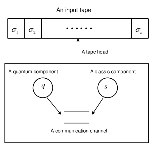
As shown in [9], there are three models of semi-quantum automata fitting into Fig. 1, with the essential difference being the specific communication pattern:

• •

  In CL-1QFA [2], only quantum-classical communication is allowed, that is, the quantum component sends its measurement result to the classical component, but no reverse communication is permitted.

• •

  In 1QFAC [13], only classical-quantum communication is allowed, that is, the classical component sends its current state to the quantum component.

• •

  In 1QCFA [15], two-way communication is allowed: (1) first, the classical component sends its current state to the quantum component; (2) second, the quantum component sends its measurement result to the classical component.

In the following, we recall the detailed definitions of the existing models of semi-quantum automata. One of such models is called one-way QFA with control language (CL-1QFA)[2], defined as follows.

In CL-1QFA ${\cal A}$, on scanning a symbol $\sigma$, a unitary operator $U_{\sigma}$ followed by the projective measurement $\mathcal{M}$ is performed on its current state. Thus, given an input string $x\in\Sigma^{*}$, the computation produces a sequence $y\in{\cal C}^{*}$ of measurement results with a certain probability $p(y|x)$ that is given by

where we define the ordered product $\prod_{i=1}^{n}A_{i}=A_{n}A_{n-1}\cdots A_{1}$. The input $x$ is said to be accepted if $y$ belongs to a fixed regular language ${\cal L}\subseteq{\cal C}^{*}$. Thus the probability of ${\cal M}$ accepting $x$ is

Recently, Qiu et al [13] proposed a new model named 1QFA together with classical states (1QFAC), defined as follows.¹¹ 1 In this paper we consider only the case that 1QFAC are language acceptors, and one can refer to [13] for a more general definition.

The machine starts with the initial states $s_{1}$ and $q_{1}$. On scanning an input symbol $\sigma\in\Sigma$, $U_{s,\sigma}$ is first applied to the current quantum state, where $s$ is the current classical state; afterwards, the classical state $s$ changes to $t=\delta(s,\sigma)$. Finally, when the whole input string is finished, a measurement ${\cal M}_{s}$ determined by the last classical state is performed on the last quantum state, and the input is accepted if the outcome $a$ is observed. Therefore, the probability of 1QFAC ${\cal A}$ accepting $x=x_{1}x_{2}\cdots x_{n}\in\Sigma^{*}$ is given by

where $s_{i+1}=\delta(s_{i},x_{i})$ for $i=1,\cdots,n$.

Ambainis and Watrous [1] proposed the model of two-way QFA with quantum and classical states (2QCFA). As proved in [1], 2QCFA can recognize non-regular language $L_{eq}=\{a^{n}b^{n}|n>0\}$ in polynomial time and the palindrome language $L_{pal}=\{x\in\{a,b\}^{*}|x=x^{R}\}$ in exponential time, which shows the superiority of 2QCFA over their classical counterparts. In the following we recall 1QCFA [15], a one-way variant of 2QCFA. Note that in this paper the notion of 1QCFA is slightly more general than the one in [15]. The reason for why we adopt the current definition is that it has a more succinct form which simplifies some notations (for example, in our version we need give only the set of general measurements, instead of two sets: unitary operators and projective measurements). It is, however, worthwhile to emphasize that all results obtained in this paper hold surely for the model in [15].

On scanning a symbol $\sigma$, at first the general measurement $\Theta_{s,\sigma}$, determined by the current classical state $s$ and the scanned symbol $\sigma$, is performed on the current quantum state, producing some outcome $c\in{\cal C}$; then the classical state $s$ changes to $s^{\prime}=\delta(s,\sigma,c)$ by reading $\sigma$ and $c$. After scanning all input symbols, ${\cal A}$ checks whether its classical state is in $S_{a}$. If yes, the input is accepted; otherwise, rejected. Therefore, the probability of 1QCFA ${\cal A}$ accepting $x=x_{1}x_{2}\cdots x_{n}\in\Sigma^{*}$ is given by

where:

• (1)

  $\chi_{a}:S\rightarrow\{0,1\}$ is defined by $\chi_{a}(s)=\left\{\begin{array}[]{ll}1,&\hbox{if $s\in S_{a}$;}\\ 0,&\hbox{otherwise.}\end{array}\right.$

• (2)

  $\{M^{c}_{s,\sigma}\}_{c\in{\cal C}}$ are measurement operators of $\Theta_{s,\sigma}$.

• (3)

  $s_{i+1}=\delta(s_{i},x_{i},c_{i})$ for $i=1,\cdots,n$.

Recall the model of MO-1gQFA which has mixed states and trace-preserving quantum operation as follows [10].

On the input word $x_{1}x_{2}\dots x_{n}\in\Sigma^{*}$, the above MO-1gQFA ${\cal A}$ proceeds as follows: the quantum operations ${\cal E}_{x_{1}},{\cal E}_{x_{2}},\dots,{\cal E}_{x_{n}}$ are performed on $\rho_{0}$ in succession, and then the projective measurement $\{P_{acc},P_{rej}\}$ is performed on the final state, obtaining the accepting result with a certain probability. Thus, MO-1gQFA ${\cal A}$ defined above induces a function ${\cal P}_{\cal A}:\Sigma^{*}\rightarrow[0,1]$ as

where ${\cal E}_{2}\circ{\cal E}_{1}(\rho)$ stands for ${\cal E}_{2}({\cal E}_{1}(\rho))$. In fact, for every $x\in\Sigma^{*}$, ${\cal P}_{\cal A}(x)$ represents the probability that ${\cal A}$ accepts $x$.

A DFA is a five-tuple ${\cal A}=(S,\Sigma,s_{1},\delta,S_{a})$ where $S$ is a finite state set, $\Sigma$ is a finite alphabet, $s_{1}\in S$ is the initial state, $S_{a}\subseteq S$ is the set of accepting states, and $\delta:S\times\Sigma\rightarrow S$ is the transition function: $\delta(s,\sigma)=t$ means that the current state $s$ changes to $t$ when scanning $\sigma$. Furthermore, $\delta$ can be extended to $\delta^{*}:S\times\Sigma^{*}\rightarrow S$ by defining: i) $\delta^{*}(s,\epsilon)=s$, and ii) $\delta^{*}(s,x\sigma)=\delta(\delta^{*}(s,x),\sigma)$ where $x\in\Sigma^{*}$ and $\sigma\in\Sigma$. ${\cal A}$ is said to accept $x\in\Sigma^{*}$, if $\delta^{*}(s_{1},x)\in S_{a}$.

Some recent work (e. g. [5, 11, 13, 16]) shows that semi-quantum automata like CL-1QFA, 1QFAC and 1QFAC are much more concise than equivalent DFA. In order to see the limit of the descriptional power of these models, size lower bounds were given in [4, 3, 13] for these models.

However, it is worth mentioning that there were some potential flaws in the procedure to obtain lower bounds for CL-1QFA in [4]. Indeed, one may find that in Lemma 5 of [4] the two states $\varphi$ and $\varphi^{\prime}$ were required to be product states, but when Lemma 5 was used to get Eq.(10) in page 110, the states $\gamma_{j,t}$ are not product states (generally, they can be entangled states). Thus, the procedure to get Eq.(10) may have a bug, whereas one can find that Eq.(10) is a crucial step, without which the lower bound may not be obtained for CL-1QFA. In the following, we present another method which can not only fix the possible bug in [4], but also deal with uniformly lower bounds on the size of 1QCFA, CL-1QFA and 1QFAC.

Before that, we first recall some preliminary knowledge. A language $L$ is said to be recognized by QFA ${\cal A}$ with cut-point $\lambda\in(0,1]$, if ${\cal P}_{\cal A}(x)>\lambda$ holds for all $x\in L$ and ${\cal P}_{\cal A}(x)\leq\lambda$ holds for all $x\notin L$. The cut-point $\lambda$ is said to be isolated whenever there exists $\delta\in(0,\frac{1}{2}]$ such that $|{\cal P}_{\cal A}(x)-\lambda|\geq\delta$, for all $x\in\Sigma^{*}$. In this case, we simply say that $L$ is recognized by ${\cal A}$ with cut-point isolated by $\delta$.

Two QFA ${\cal A}_{1}$ and ${\cal A}_{2}$ over $\Sigma$ are said to be equivalent, if ${\cal P}_{{\cal A}_{1}}(x)={\cal P}_{{\cal A}_{2}}(x)$ holds for all $x\in\Sigma^{*}$.

Below we first recall a result given in [9] that is useful for obtaining our results in this paper.

Proof. For readability, we present here the proof for CL-1QFA and one can refer to [9] for other cases. Let CL-1QFA ${\cal A}=(Q,\Sigma,{\cal C},q_{1},\{U_{\sigma}\}_{\sigma\in\Sigma},\mathcal{M},{\cal L})$, with ${\cal L}$ accepted by DFA $\mathcal{A}^{\prime}=(S,{\cal C},s_{1},\delta,S_{a})$. We construct an MO-1gQFA

from $\mathcal{A}$ and $\mathcal{A}^{\prime}$ as follows:

• •

  ${\cal H}={\cal H}_{Q}\otimes{\cal H}_{S}$ where ${\cal H}_{A}$ denotes the Hilbert space spanned by $A$;

• •

  $\rho_{0}=|q_{1}\rangle\langle q_{1}|\otimes|s_{1}\rangle\langle s_{1}|$;

• •

  ${P}_{acc}=I_{Q}\otimes\sum_{s\in S_{a}}|s\rangle\langle s|$ where $I_{Q}$ is the identity operator on ${\cal H}_{Q}$;

• •

  for each $\sigma\in\Sigma$, ${\mathcal{E}}_{\sigma}$ has operation elements $\{{E}_{\sigma}^{c,s}\}_{c\in\mathcal{C},s\in S}$ where

  $\displaystyle{E}_{\sigma}^{c,s}=P_{c}U_{\sigma}\otimes|\delta(s,c)\rangle\langle s|.$

  (27)

It is easy to verify that the collection of operators $\{{E}_{\sigma}^{c,s}\}$ satisfies the completeness condition. Furthermore, for $\rho\otimes\varrho\in L(\mathcal{H}_{Q}\otimes\mathcal{H}_{S})$, we have

where $\mathcal{F}_{c}(\varrho)=\sum_{s\in S}|\delta(s,c)\rangle\langle s|\varrho|s\rangle\langle\delta(s,c)|$.

Now let us check the behavior of $\widehat{\cal A}$ on an input string. Suppose $\widehat{\cal A}$ starts with the initial state $\rho_{0}$ and scans a symbol $\sigma$. Then the resulting state is

where $t_{c}=\delta(s_{1},c)$. In this way, after scanning a string $x=x_{1}x_{2}\cdots x_{n}\in\Sigma^{*}$, the final state is

where $|\phi_{y}\rangle=\prod_{i=1}^{n}(P_{y_{i}}U_{x_{i}})|q_{1}\rangle$ and $s_{y}=\delta^{*}(s_{1},y)$. Note that $s_{y}\in S_{a}$ iff $y\in{\cal L}$. Thus the probability of $\widehat{\cal A}$ accepting $x$ is

where $\chi_{a}(s)$ is $1$ if $s$ is in $S_{a}$ and $0$ else. Note that the above probability is equal to the one of ${\cal A}$ given in Eq. (23). Therefore, we have completed the proof.∎

Now we are in a position to give our main results.

Let $\rho_{x}={\cal E}_{x_{n}}\circ\dots\circ{\cal E}_{x_{2}}\circ{\cal E}_{x_{1}}(\rho_{0})$, i.e., the state of ${\cal M}$ after scanning the word $x$. Now, suppose that $x\not\equiv_{L}y$, that is, there exists a string $z\in\Sigma^{*}$ such that $xz\in L$ and $yz\notin L$. Then we have

for some $\lambda\in(0,1]$, where ${\cal E}_{z}$ stands for ${\cal E}_{z_{m}}\circ\dots\circ{\cal E}_{z_{2}}\circ{\cal E}_{z_{1}}$. Denote

Then we have

On the other hand, for any $x\in\Sigma^{*}$, we have

where the inequality follows from Lemma 2, the first equality holds because $\rho_{x}$ is positive semi-definite, and the second equality holds because the operations used are trace-preserving.

In summary, we obtain the following two properties:

• •

  For any $x\in\Sigma^{*}$, $vec(\rho_{x})$ lies in the unit sphere in $\mathbb{C}^{n^{2}}$.

• •

  For any two strings $x,y\in\Sigma^{*}$ satisfying $x\not\equiv_{L}y$, we always have

  $\displaystyle||vec(\rho_{x})-vec(\rho_{y})||_{tr}\geq\frac{2\delta}{\sqrt{n}}.$

  (33)

Now, suppose that $\Sigma^{*}$ consists of $d$ equivalence classes, say $[x_{1}],[x_{2}],\cdots,[x_{d}]$. Arbitrarily choose an element $vec(\rho_{x_{i}})$. Let

i.e., a sphere centered at $vec(\rho_{x_{i}})$ with the radius $\frac{\delta}{\sqrt{n}}$. Then all these spheres do not intersect pairwise except for their surface, and all of them are contained in a large sphere in $\mathbb{C}^{n^{2}}$ centered at $(0,0,\cdots,0)$ with the radius $1+\frac{\delta}{\sqrt{n}}$. Note that $\mathbb{C}^{n^{2}}$ is an $n^{2}$-dimensional complex space and each element from it can be represented by an element of $\mathbb{R}^{2n^{2}}$. Then the volume of a sphere of a radius $r$ in $\mathbb{C}^{n^{2}}$ is $cr^{2n^{2}}$ where $c$ depends only on $n$. Therefore, it holds that

This completes the proof.∎

Furthermore, we have

Therefore, based on Theorem 8 and the above theorem, we obtain a lower bound on the size of semi-quantum automata as follows.

We have presented a uniform method for obtaining the lower bound on the size of CL-1QFA, 1QFAC and 1QCFA, and this bound shows that these automata can be at most exponentially smaller than DFA. Compared with a recent work [4], our method is much more concise and universal, and it is applicable to the three existing main models of semi-quantum automata.

Note that although our lower bound is universal, it is not necessarily optimal. For instance, a better lower bound $\log d/2\log(1+\frac{\sqrt{2}}{\delta})$ was obtained for 1QFAC in [13]. Thus, a natural open problem remains either to witness the optimality of our size lower bound for some specific model, or to improve it.

The authors are thankful to Dr. Shenggen Zheng for his useful comments.

References

- [1] A. Ambainis and J. Watrous, Two-way finite automata with quantum and classical states, Theoret. Comput. Sci., 287 (2002), pp. 299-311.
- [2] A. Bertoni, C. Mereghetti, and B. Palano, Quantum Computing: 1-Way Quantum Automata, in Proceedings of the 9th International Conference on Developments in Language Theory, Lecture Notes in Comput. Sci. 2710, Springer-Verlag, Berlin, 2003, pp. 1-20.
- [3] M. P. Bianchi, C. Mereghetti., B. Palano, On the Power of One-Way Automata with Quantum and Classical States, CIAA 2014, LNCS 8587, pp. 84-97, 2014.
- [4] M. P. Bianchi, C. Mereghetti., B. Palano, Size lower bounds for quantum automata, Theoret. Comput. Sci., 551(2014), pp. 102-115.
- [5] J. Gruska, D.W. Qiu, S.G. Zheng, Generalizations of the distributed Deutsch-Jozsa promise problem, Mathematical Structures in Computer Science, minor revisions. Also arXiv:1402.7254.
- [6] R. A. Horn and C. R. Johnson, Matrix Analysis, Cambridge University Press, Cambridge, 1986.
- [7] J. E. Hopcroft and J.D. Ullman, Introduction to Automata Theory, Languages, and Computation, Addision-Wesley, New York, 1979.
- [8] A. Kondacs and J. Watrous, On the power of finite state automata, in Proceedings of the 38th IEEE Annual Symposium on Foundations of Computer Science, 1997, IEEE Computer Society, pp. 66-75.
- [9] L. Z. Li, Y. Feng, On hybrid models of quantum finite automata, J. Comput. System Sci., accepted. Also arXiv:1206.2131.
- [10] L. Z. Li and D. W. Qiu et al, Characterizations of one-way general quantum finite automata, Theoret. Comput. Sci., 419 (2012), pp. 73-91.
- [11] C. Mereghetti and B. Palano, Quantum finite automata with control language, Theoretical Informatics and Applications, 40 (2006), pp. 315-332.
- [12] M. A. Nielsen and I. L. Chuang, Quantum Computation and Quantum Information, Cambridge University Press, Cambridge, 2000.
- [13] D. W. Qiu, L. Z. Li, P. Mateus and A. Sernadas, Exponentially more concise quantum recognition of non-RMM regular languages, J. Comput. System Sci., 81 (2015), 359-375.
- [14] D. W. Qiu, L. Z. Li, P. Mateus and J. Gruska, Quantum finite automata, chapter of Handbook on Finite State based Models and Applications, editor(s): Jiacun Wang, CRC press, October 16, 2012.
- [15] S. G. Zheng, D. W. Qiu, L. Z. Li and J. Gruska, One-way finite automata with quantum and classical states, Dassow Festschrift 2012, LNCS, 7300 (2012), pp. 273-290.
- [16] S. G. Zheng, J. Gruska and D. W. Qiu, On the state complexity of semi-quantum finite automata, RAIRO-Inf. Theor. Appl., 48 (2014), pp. 187-207.