A Continued Fraction Resummation Form of Bath Relaxation Effect in the Spin-Boson Model

In a quantum dynamic process, the interaction between the system and bath leads to irreversible energy relaxation and decoherence of the quantum system. The resulting quantum dissipation can lead to rich quantum phenomena, e.g., quantum phase transition [1]. The spin-boson (Caldeira-Leggett) model is a simple but fundamental quantum system, which can be used to interpret the quantum tunneling and localization in macroscopic systems [2, 3]. Gate operations in quantum computation and quantum information are simulated by quantum dissipative dynamics of multiple spin-boson models, where each qubit is equivalent to an individual spin [4]. In the study of quantum transport, a fundamental question is to understand the transport process from a donor to an acceptor in the two-site system [5]. In the lowest order, the transfer rate is estimated using Fermi’s golden rule (FGR), proportional to the square of the site-site coupling strength. This second-order transfer rate is expressed as the Forster theory in energy transfer [6] and as the Marcus theory in electron transfer [7]. The non-Markovian relaxation of the surrounding bath can significantly slow down the transfer process compared to the second-order prediction [8, 9, 10, 11, 12, 13, 16, 15, 14, 17]. On the other hand, the transfer rate can be optimized at an intermediate dissipation strength in a biased two-site system, which can be further related to the energy transfer optimization in multi-site systems [18, 22, 23, 24, 19, 21, 20]. Within the single excitation manifold, the two-site system can be viewed as an extension of the spin-boson model, with possible variations in the boson bath and the bath spatial correlation [25, 16].

As a simple quantum model, the spin-boson model (or the equivalent two-site system) is a benchmark system for the study of quantum dynamic methodologies. In addition to the sophisticated Feynman-Vernon influence functional [26], a straightforward approach of quantum dissipation is to apply the Nakajima-Zwanzig projection operator [27, 28]. In the lowest second order, we obtain various approximate dynamic equations from different perturbed terms, e.g., the Redfield equation from the system-bath interaction [29], and the FGR rate from the site-site coupling. The noninteracting-blip approximation (NIBA) extends the FGR rate to a time-nonlocal description of the detailed time evolution [3]. To improve the NIBA prediction, the variational polaron method is a modified second-order perturbation where the perturbed term is self-consistently determined from equilibrium distribution [30, 31]. The variational polaron method is more reliable in the unbiased two-site system with a relatively fast bath. A more systematic approach beyond the second-order perturbation is to include higher-order corrections of perturbed terms, as in the quantum kinetic expansion (QKE) approach [12, 13, 14, 15, 16, 17]. In our recent paper [16], the higher-order QKE of the site-site coupling is obtained using an indirect projection operator technique for a general multi-site system. In the two-site system, all the higher-order QKE corrections arise from the bath relaxation effect, whereas in the multi-site system, the higher-order QKE corrections also include quantum interference effects.

A key theoretical concern in the QKE approach is the resummation technique of higher-order rate kernels, due to two essential reasons. The analytical and numerical difficulties quickly increase as the expansion order increases. More crucially, the QKE rate kernels can converge slowly and become divergent as the site-site coupling increases. An appropriate resummation technique can partially include corrections of all the orders using one or a few higher-order QKE rate kernels, and avoid the divergence of large site-site couplings. For the lowest-order correction, two typical resummation techniques are the Pade approximation [12, 13] and the Landau-Zener approximation [32]. With a factor of 2 difference, the Landau-Zener approximation is not reliable in the strong dissipation limit, compared to the Pade approximation. In a recent paper [33], a modified resummation approach is proposed with an optimization according to the equilibrium distribution. However, any resummation techniques in the lowest order cannot fully account for the extra knowledge of higher-order QKE rate kernels, and its prediction deviates significantly from the exact quantum dynamics at some point.

Therefore, a more general resummation technique is required to systematically include corrections from higher-order rate kernels. In Ref. [34], a generalized Pade approximation is developed, which is complicated in its mathematical formulation and practical application. Instead, we will extend the physical factorization scheme in the Pade approximation to the higher-order QKE rate kernels and obtain a simple continued fraction form, which leads to a systematic resummed quantum kinetic expansion (RQKE) method. In Section II, the derivation of the QKE approach in the two-site system (the spin-boson model) is briefly reviewed. The time-integrated QKE rates of the first three orders are numerically computed in a quantum Debye bath. In Section III, the continued fraction resummation form is developed, and the RQKE rates are numerically compared with the exact results of both unbiased and biased systems. In this paper, all the exact quantities are obtained using the hierarchy equation method  [35, 36, 37, 38]. In Section IV, the RQKE rate kernels are used to predict the detailed population evolution, and are calibrated with the exact result. In Section V, the temperature-dependent equilibrium population is calculated using the RQKE rates, which is also compared with the exact stochastic path integral result [39, 40]. In Section VI, we summarize our studies.

In this section, we briefly review the quantum kinetic expansion (QKE) approach in Ref. [16]. With respect to the single excitation manifold, the bare Hamiltonian of a multi-site system is given by $H_{\mathrm{S}}=\sum_{n}\varepsilon_{n}|n\rangle\langle n|+\sum_{n\neq m}J_{mn}|m\rangle\langle n|$, where $|n\rangle$ represents a single-excitation quantum state localized at site $n$, $\varepsilon_{n}$ is the excitation energy of site $n$, and $J_{mn}$ is the site-site coupling strength between sites $m$ and $n$. The bare Hamiltonian of the surrounding environment is given by $H_{\mathrm{B}}$. The system-bath interaction $H_{\mathrm{S}\mathrm{B}}$ is considered to be localized at each site $n$, $H_{\mathrm{S}\mathrm{B}}=\sum_{n}H_{\mathrm{S}\mathrm{B};n}|n\rangle\langle n|$. In the site basis representation $\{|n\rangle\}$, the total Hamiltonian is written as

with $H_{n}=\varepsilon_{n}+H_{\mathrm{B}}+H_{\mathrm{S}\mathrm{B};n}$. Here the simplest two-site system coupled with a harmonic bath can be mapped to the standard spin-boson model. The time evolution of the total density matrix $\rho_{\mathrm{tot}}(t)$ follows the Liouville equation, $\partial_{t}\rho_{\mathrm{tot}}(t)=-i\mathcal{L}_{\mathrm{tot}}\rho_{\mathrm{tot}}(t)$, with $\mathcal{L}_{\mathrm{tot}}=[H_{\mathrm{tot}},\cdots]$. Throughout this paper, the reduced Planck constant $\hbar$ is treated as a unit. Following the separation of population and coherence components, the total Liouville superoperator is formally expressed as a block matrix,

where the subscripts ${\mathrm{P}}$ and ${\mathrm{C}}$ denote system population and coherence, respectively. In the two-site system, the diagonal part of $\mathcal{L}_{\mathrm{tot}}$ is fully dependent on the diagonal Hamiltonian elements $H_{n}$, while the off-diagonal part of $\mathcal{L}_{\mathrm{tot}}$ arises from the site-site coupling $J$. Subsequently, we define the partial time propagation superoperators, $\mathcal{U}_{\mathrm{P}}(t)=\exp(-i\mathcal{L}_{{\mathrm{P}}}t)$ and $\mathcal{U}_{\mathrm{C}}(t)=\exp(-i\mathcal{L}_{{\mathrm{C}}}t)$, which can be interpreted as Green’s functions in the Liouville space.

An indirect projection operator approach is applied in Ref. [16] to derive the closed time evolution equation of the reduced system population $P(t)$. The initial condition is required to be a local equilibrium state, $\rho_{\mathrm{tot}}(0)=\sum_{n}p_{n}\rho^{\mathrm{eq}}_{\mathrm{B};n}|n\rangle\langle n|$, where $p_{n}$ is the initial population of site $n$, and $\rho^{\mathrm{eq}}_{\mathrm{B};n}\propto\exp(-\beta H_{n})$ is the local Boltzman density of bath. The final time evolution equation of $P(t)$ follows a time-nonlocal convolution form,

The rate kernel $\mathcal{K}(t)$ is derived as an expansion form of the site-site coupling $J$, given by $\mathcal{K}=\mathcal{K}^{(2)}+\mathcal{K}^{(3)}+\cdots$. In the two-site system, all the odd-order terms vanish, and only the even-order terms remain. Here we introduce a local equilibrium population state matrix,

and its projection matrix, $\mathcal{P}^{(0)}_{\mathrm{eq}}=\rho^{(0)}_{\mathrm{eq}}\}\mathrm{Tr}_{\mathrm{B}}\{$, where $\mathrm{Tr}_{\mathrm{B}}\{\cdots\}$ is the partial trace over bath degrees of freedom. The $2k$-th QKE rate kernel is explicitly given by

where $\delta\mathcal{U}_{\mathrm{P}}(t)=\mathcal{U}_{\mathrm{P}}(t)-\mathcal{P}^{(0)}_{\mathrm{eq}}$ is the pure dissipative propagation superoperator, vanishing in Markovian dynamics, and $\mathcal{R}(t)=\mathcal{L}_{{\mathrm{P}}{\mathrm{C}}}\mathcal{U}_{\mathrm{C}}(t)\mathcal{L}_{{\mathrm{C}}{\mathrm{P}}}$ is the population-to-population transition superoperator. Thus, high-order ($k\geq 2$) QKE rate kernels reflect dynamics of population fluctuation around the local equilibrium state due to the bath relaxation effect of $\delta\mathcal{U}_{\mathrm{P}}(t)$. Equation (9) is equivalent to the previous expression of Eq. (15) in Ref. [16], but in a more concise form. The Feynman diagram technique is applied to visualize these quantum rate kernels in Fig. 1, which is also simplified in notation compared to previous diagrams in Ref. [16]. In detail, each initial and final numbered circle represents a local equilibrium population state, $\rho^{\mathrm{eq}}_{\mathrm{B};n}|n\rangle\langle n|$, at the corresponding site $n(=1,2)$. Each intermediate dashed circle represents the dissipative propagation $[\delta\mathcal{U}_{\mathrm{P}}(t)]_{n}$ of a system-bath entangled population state, $\rho_{{\mathrm{P}};n}(t)=[\rho_{\mathrm{tot}}(t)]_{nn}$. Unlike the notation in Ref. [16], each arrowed line represents a population-to-population transition $[\mathcal{R}(t)]_{mn}$, as a density flow from population to coherence and back to population, $[\mathcal{R}(t)]_{mn}=|J_{mn}|^{2}[\mathcal{U}_{{\mathrm{C}};mn}(t)+\mathcal{U}_{{\mathrm{C}};nm}(t)]$.

The formal expression of $\mathcal{K}^{(2k)}(\tau_{2},\tau_{3},\cdots,\tau_{2k})$ in Eq. (9) is derived for an arbitrary environment, beyond the spin-boson model. Next we assume that the bath is harmonic and $H_{\mathrm{S}\mathrm{B}}$ follows a bilinear form. With the creation ($a_{i}^{+}$) and annihilation ($a_{i}$) operators for the $i$th harmonic oscillator, the bath-coupled Hamiltonian at local site $n$ reads

where the coefficient $x_{ni}$ denotes the system-bath coupling strength reduced by the frequency $\omega_{i}$ of the $i$th harmonic oscillator. The QKE rate kernels in Eq. (9) are transformed into the time correlation functions of the displacement operator, $G_{n}=\mathrm{exp}\left[\sum_{i}x_{ni}(a_{i}^{+}-a_{i})\right]$, which can be obtained by the cumulant expansion. If the bath coupling is identical at each system site, the explicit expression of the second-order rate kernel reads

where $\tilde{\varepsilon}_{nm}=\tilde{\varepsilon}_{n}-\tilde{\varepsilon}_{m}$ is the modified site excitation energy detuning with $\tilde{\varepsilon}_{n}=\varepsilon_{n}-\sum_{i}\omega_{i}x^{2}_{ni}$, and the coefficient $s_{mn}$ arises from the site-site ‘spatial’ correlation. For the standard spin-boson model, a perfectly negative correlation leads to $s_{mn(\neq m)}=4$, while for the regular energy transfer system, a $\delta$-spatial correlation leads to $s_{mn(\neq m)}=2$. Thus, the two-site system under the $\delta$-spatial correlation is equivalent to the spin-boson model with a doubled dissipation strength (reorganization energy). The time correlation function of the displacement operator excluding the spatial dependence is

where $J(\omega)=\sum_{i}\omega^{2}_{i}x^{2}_{i}\delta(\omega-\omega_{i})$ is the bath spectral density. Equation (11) is the same as the rate kernel in the NIBA approach [3], and its time integration recovers the FGR rate. In Ref. [16], the fourth-order QKE rate kernel is derived for a general multi-site system. The simplified expression of $\mathcal{K}^{(4)}(\tau_{2},\tau_{3},\tau_{4})$ for the two-site system with the $\delta$-spatial correlation is provided in Appendix A. Furthermore, we extend to the sixth-order QKE rate kernel, and the explicit expression of 16 terms is also shown in Appendix A.

Before investigating the resummation technique in next section, we numerically calculate the quantum rate kernels of the first three orders. Both unbiased and biased two-site systems are considered with $\varepsilon_{12}=0$ and $100$ cm^-1. To be compared with the calculation of the hierarchy equation [35, 36, 37, 38], a quantum bath with the Debye spectral density is applied, given by

where $\Theta(\omega)$ is the Heaviside step function of $\omega$, $\lambda$ is the reorganization energy, and $\omega_{D}$ is the Debye frequency. For simplicity, we introduce the high-temperature approximation, leading to

where $\mathrm{Sign}(t)$ is the sign function of $t$. In our calculation, the Debye frequency is $\omega^{-1}_{D}=100$ fs, and the temperature is $T=300$ K. We focus on the time-integration of rate kernels, $\mathcal{K}^{(2k)}=\int_{0}^{\infty}d\tau_{2}\cdots\int_{0}^{\infty}d\tau_{2k}\mathcal{K}^{(2k)}(\tau_{2},\cdots,\tau_{2k})$, which can be viewed as the time-integrated effective rate matrix, especially for over-damped dynamics. Since the $2k$-th rate kernel is proportional to the $2k$-th power of the site-site coupling $J$, we normalize effective rates to remove the $J$-dependence. The normalization is over the maximum value $\mathcal{K}^{(2k)}_{\mathrm{max}}$ for the biased system, and over the value of the minimum reorganization energy ($\lambda=1$ cm^-1) for the unbiased system. Due to the heavy computational duty in a multi-time integration, the Monte Carlo simulation of $10^{12}$ samples is applied to the calculation of $\mathcal{K}^{(6)}$ for convergence. Figure 2 presents the numerical results of the forward transfer rate expansions $k^{(2k)}_{A\leftarrow D}$ from the donor site 1 to the acceptor site 2, which will be used for the resummation technique in next section. We find that $k^{(2k)}_{A\leftarrow D}$ monotonically decreases with the reorganization energy $\lambda$ in the unbiased system, whereas $k^{(2k)}_{A\leftarrow D}$ is maximized in an intermediate value of $\lambda$ in the biased system.

In the previous section, we present the explicit expansion forms of rate kernels in the two-site system (the spin-boson model) using the QKE approach. For a small site-site coupling strength, the full quantum kinetic rate kernel can be obtained straightforwardly as the sum of $\mathcal{K}^{(2k)}$ up to a converged expansion order. For a large site-site coupling strength, this simple summation cannot be applied since $\mathcal{K}^{(2k)}$ diverges as the expansion order increases. Instead, a resummation technique is required for a converged result, with one or more high-order corrections of $\mathcal{K}^{(2k)}$ $(k\geq 2)$. For the leading-order QKE correction $\mathcal{K}^{(4)}$, various resummation methods, e.g., the Pade approximation [12] and the Landau-Zener approximation [32], have been well discussed previously. Although these approximations can significantly improve the second-order prediction of the NIBA approach [12, 13, 14, 15, 16, 17], a systematic resummation approach is still required to include higher-order corrections and recover the exact quantum dynamics.

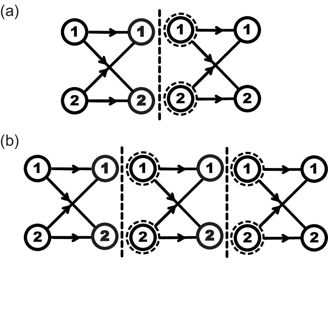
We revisit the Pade approximation in Ref. [12] to show its physical interpretation, which will used for a generalized resummation technique. As mentioned in previous section, the pure dissipation of population, $\delta\mathcal{U}_{\mathrm{P}}(t)$, vanishes in Markovian dynamics. For a fast relaxing bath with a weak non-Markovian feature, or alternatively in the strong dissipation regime where the system transport is slow but Markovian, an approximate time separation can be expected in the high-order QKE rate kernels. For the leading-order correction $\mathcal{K}^{(4)}(\tau_{2},\tau_{3},\tau_{4})$, this approximation is realized mathematically by inserting a reduced population projection $\mathcal{P}_{\mathrm{P}}$ before the action of $\delta\mathcal{U}_{\mathrm{P}}(\tau_{3})$ [12]. In the reduced population subspace, $\mathcal{P}_{\mathrm{P}}$ is explicitly written as

where $\rho^{\mathrm{eq}}_{\mathrm{B}}\propto\exp(-\beta H_{\mathrm{B}})$ is the bare bath equilibrium distribution. Equation (III) results in two identities, $\mathcal{P}_{\mathrm{P}}\mathcal{P}^{(0)}_{\mathrm{eq}}=\mathcal{P}_{\mathrm{P}}$ and $\mathcal{P}^{(0)}_{\mathrm{eq}}\mathcal{P}_{\mathrm{P}}=\mathcal{P}^{(0)}_{\mathrm{eq}}$. As a result, the fourth-order QKE rate kernel is factorized into

with $\Xi^{(2)}(\tau_{3},\tau_{4})=-\mathrm{Tr}_{\mathrm{B}}\{\mathcal{R}(\tau_{4})\delta\mathcal{U}_{\mathrm{P}}(\tau_{3})\mathcal{P}_{\mathrm{P}}\}$. The matrix factorization can be applied to all the higher-order corrections, giving

Figure 3 presents the Feynman diagrams of $\mathcal{K}^{(4)}(\tau_{2},\tau_{3},\tau_{4})$ and $\mathcal{K}^{(6)}(\tau_{2},\cdots\tau_{6})$ after the matrix factorization. With the introduction of the Laplace $z$-transform, the resummation using the correction term $\tilde{\Xi}^{(2)}(z)$ of $\tilde{\mathcal{K}}^{(4)}(z)$ becomes [12]

where $\mathcal{I}$ is an identity matrix. By expanding Eq. (20) in the $2\times 2$ matrix form, we recover the regular Pade approximation for both forward ($\tilde{k}^{(4)}_{\mathrm{resum};A\leftarrow D}(z)$) and backward ($\tilde{k}^{(4)}_{\mathrm{resum};D\leftarrow A}(z)$) transfer rate kernels.

Next we can extend to higher-order corrections with a generalized factorization technique. Following the definition of $\Xi^{(2)}(\tau_{3},\tau_{4})$ to higher-orders, we introduce another expansion series,

which is essential for the QKE in the system-bath separated initial condition [41]. For the sixth-order QKE rate kernel, a more accurate matrix factorization is changed to $\mathcal{K}^{(6)}(\tau_{2},\cdots,\tau_{6})\approx\Xi^{(4)}(\tau_{3},\cdots,\tau_{6})\mathcal{K}^{(2)}(\tau_{2})$. Similar to the cumulant expansion, the ‘real’ fourth-order correction $\Xi^{(4)}$ needs to exclude the contribution of $\Xi^{(2)}$,

All the other higher-order QKE rate kernels are subsequently factorized using $\Xi^{(2)}$ and $\delta\Xi^{(4)}$. For conciseness, we introduce the difference of $\delta\Xi^{(4)}$ relative to $\Xi^{(2)}$, which is defined in the Laplace $z$-space as

Here the expansion index 4 is assigned as a subscript since $\tilde{\Delta}_{4}(z)$ is in the same $J$-expansion order as $\tilde{\Delta}_{2}(z)=\tilde{\Xi}^{(2)}(z)$. The approximate full quantum rate kernel resummed from $\tilde{\Delta}_{2}(z)$ and $\tilde{\Delta}_{4}(z)$ is derived in a continued fraction form,

The above factorization scheme can be straightforwardly to an arbitrary expansion order, which defines the general correction term, $\delta\tilde{\Xi}^{(2k)}(z)=\tilde{\Delta}_{2k-2}(z)\cdots\tilde{\Delta}_{2}(z)$, and gives rise to the general matrix continued fraction form.

The separation of higher-order QKE rate kernels depicted in Fig. 3 requires modifications when the non-Markovian dynamics is not weak. The dynamic coupling between $\Xi^{(2k-2)}(\tau_{3},\cdots,\tau_{2k})$ and $\mathcal{K}^{(2)}(\tau_{2})$ needs to be include, beyond the matrix factorization, $\mathcal{K}^{(2k)}(\tau_{2},\cdots,\tau_{2k})\approx\Xi^{(2k-2)}(\tau_{3},\cdots,\tau_{2k})\mathcal{K}^{(2)}(\tau_{2})$. However, this difficulty can be circumvented using the scalar continued fraction form for each element of the rate kernel. Mathematically, a regular function can be re-expressed in the continued fraction form, by matching its Taylor expansion series. Thus, we propose the scalar continued fraction resummation form for the forward rate kernel,

where the correction terms are matching the QKE forward rate kernels $\tilde{k}^{(2j)}_{A\leftarrow D}(z)$ term by term, given by

The same approach is applied to resum the backward rate kernel $\tilde{k}^{(2k)}_{\mathrm{resum};D\leftarrow A}(z)$. Equations (25)-(27) provides the basic construction of the resummed quantum kinetic expansion (RQKE) method. To be consistent, the expansion order of the RQKE is defined by the power of the site-site coupling strength in the highest-order QKE rate kernel considered. Compared to the generalized Pade approximation in Ref. [34], the continued fraction can also be expanded into a rational polynomial form, while the correction terms in the RQKE method are more straightforwardly obtained without an additional basis expansion. In addition, as the resummation order $2k$ increases, all the lower-order correction terms $\tilde{\delta}_{2j(<k-1)}(z)$ are not affected, which makes the continued fraction form a more systematic approach.

To verify the reliability of the continued fraction form, we use the results of the first three order effective rate expansions in Section II to obtain the RQKE rates $k^{(2k)}_{\mathrm{resum}}=\tilde{k}^{(2k)}_{\mathrm{resum}}(z=0)$, which are compared with the exact full quantum rates $k_{\mathrm{exact}}$ from the hierarchy equation. In Ref. [16], $k_{\mathrm{exact}}$ is calculated under a system-bath separated initial condition, different from the presumption of the local equilibrium population state in the QKE approach. The accurate value of $k_{\mathrm{exact}}$ is re-calculated, following the rigorous expression in Ref. [41]. With the same equilibrium population, the results of $k_{\mathrm{exact}}$ under these two initial conditions are proportional to each other [41]. The results of $k^{(2)}$, $k^{(4)}_{\mathrm{resum}}$, $k^{(6)}_{\mathrm{resum}}$, and $k_{\mathrm{exact}}$ for the forward transport process form the donor site 1 to the acceptor site 2 are plotted in Figs. 4 and 5. For the unbiased system ($\varepsilon_{12}=0$), two site-site coupling strengths, $J=40$ and $100$ cm^-1 are considered; for the biased system ($\varepsilon_{12}=100$ cm^-1), two site-site coupling strengths, $J=20$ and $100$ cm^-1 are considered. For the two small site-site coupling strengths, $J=40$ cm^-1 and $\varepsilon_{12}=0$ in Fig. 4a, and $J=20$ cm^-1 and $\varepsilon_{12}=100$ cm^-1 in Fig. 5a, the QKE rate kernels converge with the expansion order. The lowest fourth-order RQKE rate $k^{(4)}_{\mathrm{resum};A\leftarrow D}$ improves the second-order FGR rate and predict $k_{\mathrm{exact};A\leftarrow D}$ accurately in the whole range of the reorganization energies, $1$ cm${}^{-1}\leq\lambda\leq 1000$ cm^-1. For the large coupling strength of $J=100$ cm^-1 in Figs. 4b and 5b, the QKE rate kernels diverge with the expansion order. In the unbiased system, $k^{(4)}_{\mathrm{resum};A\leftarrow D}$ improves $k^{(2)}_{A\leftarrow D}$ mainly in the large-$\lambda$ regime. In the biased system, $k^{(4)}_{\mathrm{resum};A\leftarrow D}$ largely improves $k^{(2)}_{A\leftarrow D}$, except for a small deviation in the intermediate-$\lambda$ regime. In Fig. 5b of Ref. [16], the difference between $k^{(4)}_{\mathrm{resum};A\leftarrow D}$ and $k_{\mathrm{exact};A\leftarrow D}$ in the large-$\lambda$ regime is due to an inconsistent initial condition in the hierarchy equation. For both cases, the next sixth-order RQKE rate $k^{(6)}_{\mathrm{resum};A\leftarrow D}$ agrees perfectly with $k_{\mathrm{exact};A\leftarrow D}$ in the whole $\lambda$ regime. Our numerical calculations demonstrate that the RQKE rate from the continued fraction form can systematically approach to the exact value, and the number of necessary correction terms gradually increase with the site-site coupling strength.

The continued fraction form of the bath relaxation effect is verified by the convergence of the resummed effective rate toward the exact value. In this section, we will further demonstrate the accuracy of the continued fraction in predicting the detailed time evolution of site population.

All the high-order QKE rate kernels can be derived explicitly, using the cumulant expansion for the multi-time correlation function of the displacement operator. The time evolution of reduced site population $P(t)$ is subsequently solved by the convoluted equation in the time $t$-space, or equivalently by the matrix inversion in the Laplace $z$-space. The computational cost of both methods is often very high. Instead, we re-express the QKE rate kernels in a matrix formalism [41]. The general $2k$-th QKE rate kernel in the Laplace $z$-space is derived in Ref. [41] as

with $\tilde{\bm{\mathcal{R}}}(z)=\bm{\mathcal{W}}^{(1)}\delta\tilde{\bm{\mathcal{U}}}^{(0)}(z)\bm{\mathcal{W}}^{(1)}$. Here each matrix is defined in an expanded basis set of relevant dynamic variables and can be mapped to a superoperator in Section II. Specifically, the mapping of two projection matrices are $\mathcal{P}_{\mathrm{P}}\Leftrightarrow\bm{\mathcal{P}}_{\mathrm{P}}$ and $\mathcal{P}^{(0)}_{\mathrm{eq}}\Leftrightarrow\bm{\mathcal{P}}^{(0)}_{\mathrm{eq}}$. The two interaction Liouville superoperators are combined together and mapped to a perturbed transition rate matrix, $\{i\mathcal{L}_{{\mathrm{P}}{\mathrm{C}}},i\mathcal{L}_{{\mathrm{C}}{\mathrm{P}}}\}\Leftrightarrow\bm{\mathcal{W}}^{(1)}$. The two unperturbed time propagation superoperaotrs are also combined together and mapped to an unperturbed pure dissipative matrix, $\{\delta\tilde{\mathcal{U}}_{\mathrm{P}}(z),\tilde{\mathcal{U}}_{\mathrm{C}}(z)\}\Leftrightarrow\delta\tilde{\bm{\mathcal{U}}}^{(0)}(z)$.

For over-damped quantum dynamics in the two-site system, the time evolution of site population is close to a single exponential decaying function (Markovian behavior), which can be described by the time-integrated effective rate. To illustrate the relevant non-Markovian behavior, we focus on small and intermediate reorganization energies with under-damped dynamics. In our two-site system, we choose two typical reorganization energies, $\lambda=4$ and $12$ cm^-1, for each system condition ($\varepsilon_{12}$ and $J$) in Figs. 4 and 5. The exact time evolution of site population, $P_{\mathrm{exact};1}(t)$, is solved by the hierarchy equation using the local equilibrium population state initially at the donor site 1. Next we re-calculate the site population $\tilde{P}_{\mathrm{exact};1}(z)$ in the Laplace $z$-space, and obtain a new estimation of the time evolution, $P^{\prime}_{\mathrm{exact};1}(t)=\mathrm{LT}^{-1}[\tilde{P}_{\mathrm{exact};1}(z)]$, using the inverse Laplace transform, $\mathrm{LT}^{-1}[\cdots]$. The two time evolution predictions, $P_{\mathrm{exact};1}(t)$ and $P^{\prime}_{\mathrm{exact};1}(t)$ are found to be identical, confirming the reliability of the numerical inverse Laplace transform. In our model system, Eq. (28) is also numerically solved using the hierarchy equation approach [41]. The estimation of the site population from the $2k$-th order RQKE rate kernel is written as

We apply the same two-site system with the same quantum Debye bath with $\omega^{-1}_{D}=100$ fs and $T=300$ K in previous two sections. The comparison between $P^{(2)}_{1}(t)$, $P^{(2k)}_{\mathrm{resum};1}(t)$ and $P_{\mathrm{exact};1}(t)$ is organized in Figs. 6 and 7, where $P^{(2)}_{1}(t)$ is the second-order NIBA prediction. In the unbiased system ($\varepsilon=0$) with the small site-site coupling ($J=40$ cm^-1), $P^{(2)}_{1}(t)$ is close to the exact time evolution $P_{\mathrm{exact};1}(t)$ with a small deviation. The lowest fourth-order RQKE rate kernel, $\tilde{\mathcal{K}}^{(4)}_{\mathrm{resum}}(z)$, further improves $P^{(2)}_{1}(t)$ and provides almost identical results of $P_{\mathrm{exact};1}(t)$ for the two reorganization energies. As the site-site coupling is increased to $J=100$ cm^-1, $P^{(4)}_{\mathrm{resum};1}(t)$ improved from the NIBA prediction also deviates from the exact result $P_{\mathrm{exact};1}(t)$. We find that $P^{(2k)}_{\mathrm{resum};1}(t)$ gradually approaches to $P_{\mathrm{exact};1}(t)$ as the $J$-expansion order $2k$ increases in the continued fraction form. As shown in Figs. 6c and d, $P^{(8)}_{\mathrm{resum};1}(t)$ and $P^{(6)}_{\mathrm{resum};1}(t)$ from the eighth- and sixth-order RQKE rate kernels fully recover $P_{\mathrm{exact};1}(t)$ for $\lambda=4$ and $12$ cm^-1, respectively. In the biased system ($\varepsilon=100$ cm^-1) with the small site-site coupling ($J=20$ cm^-1), $P^{(2)}_{1}(t)$ clearly deviates from $P_{\mathrm{exact};1}(t)$, while $P^{(4)}_{\mathrm{resum};1}(t)$ from the Pade approximation becomes almost identical to $P_{\mathrm{exact};1}(t)$ for the two values of $\lambda$. Although the time-integrated rate $k^{(4)}_{\mathrm{resum}}$ is very close to the exact value $k_{\mathrm{exact}}$ in the small-$\lambda$ regime, the prediction of $P^{(4)}_{\mathrm{resum};1}(t)$ is no longer reliable for the strong site-site coupling ($J=100$ cm^-1). Similarly, we extend the continued fraction form to higher orders, and $P^{(10)}_{\mathrm{resum};1}(t)$ from the tenth-order RQKE rate kernel fully recovers $P_{\mathrm{exact};1}(t)$ for $\lambda=4$ and $12$ cm^-1. Thus, the exact quantum dynamics can be fully predicted by the RQKE rate kernels in the continued fraction form. The convergence order of the continued fraction for the detailed time evolution in general increases as the reorganization energy decreases. Since the equilibrium population in the unbiased system is unchanged with the system and bath parameters, the convergence order is usually smaller than that in the biased system.

In this section, we will further demonstrate the accuracy of the continued fraction in predicting the temperature dependence of quantum equilibrium population.

In the original matrix continued fraction form, the expansion $\tilde{\Xi}^{(2k)}(z)$ from the factorization scheme on the high-order QKE rate kernels leads to the same correction terms for both forward and backward transfer rate kernels, i.e., $\tilde{\delta}_{2k;A\leftarrow D}(z)=\tilde{\delta}_{2k;D\leftarrow A}(z)$. The ratio of the two time-integrated RQKE rates, $k^{(2k)}_{\mathrm{resum};A\leftarrow D}/k^{(2k)}_{\mathrm{resum};D\leftarrow A}$, is unchanged as the resummation order increases. The equilibrium population is always the same as the classical Boltzmann distribution of the FGR prediction, $P_{\mathrm{eq};n}\propto\exp(-\beta\varepsilon_{n})$, which is only valid at high temperatures. In our modified scalar continued fraction form, the correction terms of the forward and backward rate kernels are determined independently, which allows $\tilde{\delta}_{2k;A\leftarrow D}(z)\neq\tilde{\delta}_{2k;D\leftarrow A}(z)$. Consequently, the equilibrium population predicted by the RQKE rate can deviate from the classical Boltzmann distribution and approach to the exact quantum Boltzmann distribution, $P_{\mathrm{eq};n}\propto[\mathrm{Tr}_{B}\{\exp(-\beta H_{\mathrm{tot}})\}]_{nn}$ [39, 40].

As a verification, we extend our previous study at a high temperature $T=300$ K to lower temperatures. Since the equilibrium population is always one half in the unbiased system, we only consider the biased system, $\varepsilon_{12}=100$ cm^-1 with $J=100$ cm^-1 and $\lambda=100$ cm^-1. The $2k$-th order prediction of the donor equilibrium population $P^{(2k)}_{\mathrm{eq};\mathrm{resum};1}$ is obtained using the time-integrated RQKE rates,

The full expression of the time correlation function $g(t)$ is applied in the calculation of the QKE rate kernels, without the high-temperature approximation. Similarly, $10^{12}$ Monte Carlo samples are simulated for an accurate estimation of $k^{(6)}_{\mathrm{resum}}$. The hierarchy equation with the Matsubara frequency summation is used to obtain the exact equilibrium population, which is numerically the same as the result of the stochastic path integral [39, 40]. Our numerical calculation shows that each correction term $\delta_{2j(<k-1)}$ is different for the forward and backward rates, and the deviation increases as temperature decreases. As shown in Fig. 8, the RQKE rates systematically improves the prediction of $P^{(2k)}_{\mathrm{eq};\mathrm{resum};1}$ from the second-order FGR result to the exact result. With specific parameters in our calculation, the sixth-order RQKE rates provide an excellent prediction of the exact result over the whole temperature range (100 K $\leq T\leq 300$ K). With more correction terms included, we expect that the scalar continued fraction resummation can be straightforwardly extended to lower temperatures.

In this paper, we extend our previous study of the quantum kinetic expansion (QKE) approach in the two-site system (the spin-boson model). The factorization scheme for the high-order QKE rate kernels in the weak non-Markovian dynamics leads to the matrix continued fraction form for the resummation technique of QKE rate kernels. To be valid in an arbitrary condition, we further introduce the scalar continued fraction form for forward and backward rate kernels separately, where the correction terms are obtained by matching the higher-order QKE rate kernels. Consequently, a systematic resummed quantum kinetic expansion (RQKE) method is constructed, and the expansion order of the RQKE method is consistent with the highest order of the QKE rate kernel. To the lowest fourth-order, the continued fraction form recovers the Pade approximation, while the higher-order RQKE correction terms represent the additional bath relaxation effects. As shown by numerical calculations in this paper, the prediction of the RQKE method systematically improves with the expansion order and can fully reproduce the exact quantum dynamics calculated from the hierarchy equation. With specific parameters considered in this paper, the time-integrated RQKE rate at the sixth order can be almost identical to the exact result for both unbiased and biased system, with both weak and strong site-site coupling strengths. More importantly, the detailed time evolution can be exactly predicted as well, as higher-order correction terms are gradually included. The temperature dependence of the equilibrium population is also verified, as the classical Boltzmann distribution of the second-order FGR prediction is improved toward the exact quantum Boltzmann distribution. The convergence order generally increases with the increase of the site-site coupling strength, the decrease of the reorganization energy and the decrease of temperature.

The numerical calculations of this paper are focused on the harmonic bath with a quantum Debye spectral density. The formal expression of the QKE rate kernel in Eq. (9) is however invariant of the bath structure, whether Gaussian or non-Gaussian, so that the RQKE method can be applied to a general bath, combined with other numerical methods. The mathematical strategy of applying the continued fraction form is not limited to the two-site system, and its application to more complicated systems will be demonstrated in our forthcoming papers. The RQKE method provides a systematically converged approach of quantum dynamics, and its continued fraction form can inspire possibilities of other higher-order resummation techniques, such as the extension of the Landau-Zener approximation and modifications originally for the lowest order correction.

References

- [1] S. Sachdev, Quantum Phase Transitions (Cambridge University Press, New York, 2011).
- [2] A. O. Caldeira and A. J. Leggett, Phys. Rev. Lett. 46, 211 (1981).
- [3] A. J. Leggett, S. Chakravarty, A. T. Dorsey, M. P. A. Fisher, A. Garg, and W. Zwerger, Rev. Mod. Phys. 59, 1 (1987).
- [4] H. P. Breuer and F. Petruccione, The Theory of Open Quantum Systems (Oxford University Press, New York, 2002).
- [5] A. Nitzan, Chemical Dynamics in Condensed Phases: Relaxation, Transfer and Reactions in Condensed Molecular Systems (Oxford University Press, New York, 2006).
- [6] T. Förster, Ann. Phys. (Leipzig) 437, 55 (1948).
- [7] R. A. Marcus, Annu. Rev. Phys. Chem. 15, 155 (1964).
- [8] L. D. Zusman, Chem. Phys. 49, 295 (1980).
- [9] H. Sumi and R. A. Marcus, J. Chem. Phys. 84, 4894 (1986).
- [10] J. S. Cao and Y. Jung, J. Chem. Phys. 112, 4716 (2000).
- [11] R. F. Loring and S. Mukamel, J. Chem. Phys. 87, 1272 (1987).
- [12] M. Sparpaglione and S. Mukamel, J. Chem. Phys. 88, 3263 (1988).
- [13] Y. Hu and S. Mukamel, J. Chem. Phys. 91 , 6973 (1989).
- [14] B. B. Laird, J. Budimir, and J. L. Skinner, J. Chem. Phys. 94, 4391 (1991).
- [15] J. S. Cao, J. Chem. Phys. 112, 6719 (2000).
- [16] J. L. Wu and J. S. Cao, J. Chem. Phys. 139, 044102 (2013).
- [17] D. R. Reichman and R. J. Silbey, J. Chem. Phys. 104, 1506 (1996)
- [18] J. S. Cao and R. J. Silbey, J. Phys. Chem. A 113, 13825 (2009).
- [19] J. L. Wu, F. Liu, Y. Shen, J. S. Cao, and R. J. Silbey, New J. Phys. 12, 105012 (2010).
- [20] J. Moix, J. L. Wu, P. F. Huo, D. Coker, and J. S. Cao, J. Phys. Chem. Lett. 2, 3045 (2011).
- [21] J. L. Wu, F. Liu, J. Ma, R. J. Silbey, and J. S. Cao, J. Chem. Phys. 137, 174111 (2012).
- [22] J. L. Wu, R. J. Silbey, and J. S. Cao, Phys. Rev. Lett. 110, 200402 (2013).
- [23] M. B. Plenio and S. F. Huelga, New J. Phys. 10, 113019 (2008).
- [24] P. Rebentrost, M. Mohseni, I. Kassal, S. Lloyd, and A. Aspuru-Guzik, New J. Phys. 11, 033003 (2009).
- [25] V. May and K. Oliver, Charge and Energy Transfer Dynamics in Molecular Systems (Wiley-VCH, Weinheim, 2004).
- [26] R. P. Feynman and F. L. Vernon, Jr., Ann. Phys. (N.Y.) 24, 118 (1963).
- [27] S. Nakajima, Prog. Theor. Phys. 20, 948 (1958).
- [28] R. Zwanzig, J. Chem. Phys. 33, 1338 (1960).
- [29] A. G. Redfield, IBM J. Res. Dev. 19, 1 (1957).
- [30] R. J. Silbey and R. A. Harris, J. Chem. Phys. 80, 2615 (1984).
- [31] C. Wang, J. Ren, and J. S. Cao, arXiv:1410.4366 (2014)
- [32] H. Sumi, J. Phys. Soc. Jpn. 49, 1701 (1980)
- [33] M. G. Mavros and T. V. Voorhis, J. Chem. Phys. 141, 054112 (2014).
- [34] M. Cho and R. J. Silbey, J. Chem. Phys. 106, 2654 (1997).
- [35] Y. Tanimura and R. Kubo, J. Phys. Soc. Jpn. 58, 101 (1989).
- [36] Y. Yan, F. Yang, Y. Liu, and J. Shao, Chem. Phys. Lett. 395, 216 (2004).
- [37] R. X. Xu, P. Cui, X. Q. Li, Y. Mo, and Y. J. Yan, J. Chem. Phys. 122, 041103 (2005).
- [38] J. M. Moix and J. Cao, J. Chem. Phys. 139, 134106 (2013).
- [39] C. K. Lee, J. Moix and J. S. Cao, J. Chem. Phys. 136, 204120 (2012).
- [40] J. M. Moix, Y. Zhao, and J. S. Cao, Phys. Rev. B 85, 115412 (2012).
- [41] J. L. Wu, in preparation.